A Comprehensive Guide to ChIP-Seq Data Analysis for Histone Modifications: From QC to Chromatin State Annotation

Abstract

This article provides a complete workflow for analyzing ChIP-seq data focused on histone modifications, tailored for researchers and drug development professionals. It covers foundational concepts of histone mark biology and epigenomics, a step-by-step methodological pipeline from quality control to peak calling and annotation, essential troubleshooting and optimization strategies for common pitfalls, and finally, rigorous validation and comparative analysis techniques. By integrating current best practices and standards from consortia like ENCODE, this guide empowers scientists to reliably interpret the epigenomic landscape and its implications in gene regulation and disease.

Understanding Histone Modifications and Epigenomic Landscapes

Histone modifications are post-translational modifications (PTMs) of histone proteins that serve as fundamental epigenetic mechanisms for regulating gene expression and chromatin structure in eukaryotes [1]. These modifications occur on the core histone proteins (H2A, H2B, H3, and H4) that form the nucleosome octamer around which DNA is wrapped [2]. The N-terminal tails of histones, which protrude from the nucleosome core, are particularly rich sites for modifications that alter chromatin accessibility and serve as binding platforms for downstream effector proteins [1] [3].

These PTMs play pivotal roles in various cellular processes including transcriptional regulation, DNA repair, DNA replication, and genome stability maintenance [1] [3]. The combinatorial nature of histone modifications creates a complex "histone code" that can be interpreted by reader proteins to elicit specific chromatin states and functional outcomes [1] [2]. Irregularities in histone PTMs are increasingly recognized as contributors to various diseases, including cancer, degenerative disorders, and abnormal developmental phenotypes [4] [5].

Major Types of Histone Modifications and Their Functions

Common Histone Modification Types

Histone modifications encompass a diverse array of chemical groups that can be added or removed from specific amino acid residues. The major types include methylation, acetylation, phosphorylation, and ubiquitination, among others [5]. The CHHM database, a manually curated catalogue of human histone modifications, documents 31 distinct types of modifications plus histone-DNA crosslinks, identified across numerous histone variants [2].

The functional consequence of each modification depends on both the specific residue modified and the type of modification installed. For example, methylation can have either activating or repressive effects depending on the position of the methylated residues and the degree of methylation (mono-, di-, or tri-methylation) [1]. Acetylation generally counteracts the positive charge of lysine residues, leading to a more open chromatin structure [4].

Genomic Distributions and Biological Functions

Table 1: Major Histone Modifications, Their Genomic Distributions and Biological Functions

Modification	Associated Chromatin State	Primary Genomic Location	Biological Function
H3K4me3	Euchromatin	Promoter regions [6]	Transcriptional activation [1]
H3K4me1	Euchromatin	Enhancer regions [6]	Enhancer identification [2]
H3K9me3	Constitutive Heterochromatin	Repetitive regions, TE-rich regions [1] [7]	Transcriptional repression, TE silencing [1] [5]
H3K27me3	Facultative Heterochromatin	Promoters of developmentally regulated genes [1] [6]	Developmental gene regulation [1] [5]
H3K27ac	Active Regulatory Elements	Enhancers and promoters [8]	Active enhancer marking [8]
H3K36me3	Transcriptionally Active Regions	Gene bodies of actively transcribed genes [3] [6]	Transcriptional elongation [6]
H3K9ac	Euchromatin	Promoter regions [6]	Transcriptional activation [6]

The genome is broadly divided into euchromatin (less compact, transcriptionally active) and heterochromatin (condensed, transcriptionally repressive), with distinct histone modifications characterizing each state [3]. Euchromatin is typically enriched with histone acetylation and H3K4 methylation, while heterochromatin is marked by H3K9me3 and H3K27me3 [3]. Recent research has revealed further complexity within these broad categories, identifying distinct subcompartments such as K4-facultative heterochromatin (adjacent to euchromatin) and K9-facultative heterochromatin (adjacent to constitutive heterochromatin), each with unique functional properties [1].

Figure 1: Functional Consequences of Major Histone Modifications. Histone modifications alter chromatin structure and recruit effector proteins to drive specific functional outcomes.

Histone Modification Analysis by ChIP-Seq

ChIP-Seq Workflow and Methodology

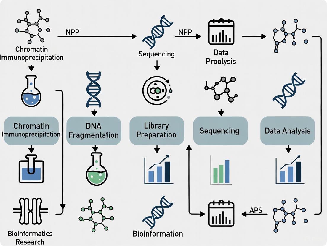
Chromatin Immunoprecipitation followed by sequencing (ChIP-seq) is the method of choice for genome-wide analysis of histone modifications [6] [9]. This technique provides a snapshot of histone-DNA interactions in a given cell type, developmental stage, or disease condition [6]. The standard ChIP-seq workflow involves multiple critical steps:

Crosslinking and Cell Lysis: Proteins are crosslinked to their genomic DNA substrates in living cells using formaldehyde. Cells are then lysed to release chromatin [6].

Chromatin Fragmentation: Chromatin is fragmented to mononucleosome-sized fragments, typically by sonication or micrococcal nuclease (MNase) digestion. Sonication is preferred for mapping transcription factors, while MNase digestion results in more uniform mono-nucleosome sized fragments and higher resolution for histone modifications [10].

Immunoprecipitation: Specific histone modifications are precipitated using validated antibodies. The quality and specificity of antibodies are critical factors for successful ChIP-seq experiments [7] [6].

Library Preparation and Sequencing: After reversal of crosslinks, the ChIP DNA is purified and used to prepare sequencing libraries. The Illumina platform is most commonly used for ChIP-seq studies [6].

Data Analysis: Sequence reads are aligned to a reference genome, and enriched regions are identified using peak-calling algorithms. For histone modifications with broad domains like H3K27me3 and H3K9me3, specialized algorithms such as SICER or ChromaBlocks are required [10].

Figure 2: ChIP-seq Experimental Workflow. Key steps in the ChIP-seq protocol for mapping histone modifications genome-wide.

ChIP-Seq Standards and Quality Control

The ENCODE consortium has established comprehensive standards for ChIP-seq experiments to ensure data quality and reproducibility [7]. Key standards include:

• Biological Replicates: Experiments should include two or more biological replicates [7].
• Antibody Validation: Antibodies must be thoroughly characterized according to ENCODE standards [7].
• Input Controls: Each ChIP-seq experiment should have a corresponding input control with matching replicate structure [7] [10].
• Sequencing Depth: For broad histone marks like H3K27me3, each replicate should have 45 million usable fragments, while narrow marks require 20 million fragments per replicate [7]. H3K9me3 represents an exception due to its enrichment in repetitive regions [7].
• Library Complexity: Preferred values are NRF>0.9, PBC1>0.9, and PBC2>10 [7].

Quality control metrics should be collected to determine library complexity, read depth, FRiP score (Fraction of Reads in Peaks), and reproducibility [7].

Analytical Approaches for Histone Modification Data

Different analytical approaches are required depending on the nature of the histone modification being studied. Modifications with sharp, punctate distributions (e.g., H3K4me3) can be analyzed using algorithms designed for peak calling, such as MACS [10]. In contrast, modifications with broad genomic footprints (e.g., H3K27me3, H3K9me3) require specialized tools like SICER, ChromaBlocks, or histoneHMM that can identify large enriched domains [10] [5].

For differential analysis between conditions, several methods have been developed specifically for broad histone marks. The histoneHMM algorithm uses a bivariate Hidden Markov Model to classify genomic regions as modified in both samples, unmodified in both samples, or differentially modified between samples [5]. This approach has been shown to outperform methods designed for peak-like features when analyzing broad histone modifications [5].

The Scientist's Toolkit: Essential Research Reagents and Materials

Table 2: Key Research Reagents and Materials for Histone Modification Studies

Reagent/Material	Specification/Example	Function/Application
Histone Modification Antibodies	H3K4me3 (CST #9751S), H3K27me3 (CST #9733S), H3K9me3 (CST #9754S) [6]	Immunoprecipitation of specific histone modifications
Crosslinking Reagent	Formaldehyde solution (37% w/w) [6]	Crosslinks proteins to DNA in living cells
Cell Lysis Buffer	5 mM PIPES pH 8, 85 mM KCl, 1% igepal [6]	Cell membrane disruption and chromatin release
Nuclei Lysis Buffer	50 mM Tris-HCl pH 8, 10 mM EDTA, 1% SDS [6]	Nuclear membrane disruption
Chromatin Shearing Instrument	Bioruptor UCD-200 (Diagenode) or equivalent [6]	Chromatin fragmentation to mononucleosome size
Protease Inhibitors	Aprotinin, Leupeptin, PMSF [6]	Prevent protein degradation during processing
IP Dilution Buffer	50 mM Tris-HCl pH 7.4, 150 mM NaCl, 1% igepal, 0.25% deoxycholic acid, 1 mM EDTA [6]	Dilution of chromatin before immunoprecipitation
DNA Purification Kit	QIAquick PCR purification kit (QIAGEN) [6]	Purification of ChIP DNA after crosslink reversal
SM30 Protein	SM30 Protein|Sea Urchin Spicule Matrix Protein	SM30 Protein is a key matrix protein from sea urchin spicules, vital for biomineralization studies. For Research Use Only. Not for human or veterinary use.
N-Butyl Nortadalafil	N-Butyl Nortadalafil (CAS 171596-31-9) - Tadalafil Analog	N-Butyl Nortadalafil is a high-purity Tadalafil analog for PDE5 inhibitor research. For Research Use Only. Not for human or veterinary use.

Advanced Applications and Recent Technological Developments

Single-Cell Histone Modification Analysis

Traditional ChIP-seq requires thousands to millions of cells, masking cellular heterogeneity within samples. Recent advances have enabled single-cell analysis of histone modifications, providing unprecedented resolution for studying epigenetic heterogeneity. The TACIT (Target Chromatin Indexing and Tagmentation) method enables genome-coverage single-cell profiling of multiple histone modifications simultaneously [8].

TACIT has been applied to profile seven histone modifications (H3K4me1, H3K4me3, H3K27ac, H3K27me3, H3K36me3, H3K9me3, and H2A.Z) across mouse early embryo development, revealing cellular heterogeneity and epigenetic reprogramming at single-cell resolution [8]. Further development led to CoTACIT (Combined TACIT), which can profile multiple histone modifications in the same single cell through sequential rounds of antibody binding and tagmentation [8].

These single-cell technologies have revealed that histone modification heterogeneity emerges as early as the two-cell stage in mouse embryos, with H3K27ac profiles showing marked heterogeneity at this stage compared to other modifications [8]. This finding suggests that cells may begin to establish functional heterogeneity immediately after zygotic genome activation.

Integrative Analysis and Chromatin State Annotation

Combining multiple histone modification profiles enables comprehensive annotation of chromatin states across the genome. This approach has been powerfully applied to identify regulatory elements and characterize their dynamics during development and disease [8] [9].

By integrating profiles of six histone modifications with single-cell RNA sequencing data, researchers have developed models that predict the earliest cell lineage branching events during embryonic development and identify novel lineage-specifying transcription factors [8]. Such integrative approaches provide insights into how combinatorial histone modification patterns contribute to cell fate decisions.

Several curated databases provide comprehensive information about histone modifications. The CHHM (Catalogue of Human Histone Modifications) database is a manually curated resource containing 6,612 non-redundant modification entries covering 31 types of modifications and 2 types of histone-DNA crosslinks [2]. This database reveals modification hotspot regions and uneven distribution patterns across histone families, providing insights into the specificity of different modification types [2].

Other valuable resources include the ENCODE Consortium, which provides standardized ChIP-seq data and protocols [7], and specialized tools like PTMViz, which offers an interactive platform for analyzing differential abundance of histone PTMs from mass spectrometry data [4].

Histone modifications represent a crucial layer of epigenetic regulation that controls chromatin structure and function. The development of ChIP-seq technologies has enabled comprehensive mapping of these modifications genome-wide, revealing their complex distributions and functional relationships. As single-cell methods and integrative analytical approaches continue to advance, our understanding of how histone modification patterns contribute to cellular identity, lineage specification, and disease pathogenesis will continue to deepen. The standardized protocols, curated databases, and specialized analytical tools described herein provide researchers with essential resources for exploring the fascinating world of histone modifications and their functional consequences.

Chromatin Immunoprecipitation followed by sequencing (ChIP-seq) is a powerful method for analyzing protein interactions with DNA on a genome-wide scale. This technology combines the specificity of chromatin immunoprecipitation with the comprehensive nature of high-throughput DNA sequencing to precisely map the binding sites of DNA-associated proteins. ChIP-seq has revolutionized epigenetic research by enabling researchers to capture the genomic locations of transcription factors, histone modifications, and chromatin-modifying complexes with unprecedented resolution and sensitivity [11].

The fundamental principle underlying ChIP-seq involves the cross-linking of proteins to DNA in living cells, followed by fragmentation of chromatin and immunoprecipitation of the protein-DNA complexes using specific antibodies. The immunoprecipitated DNA is then purified, sequenced, and mapped to a reference genome to identify enriched regions, known as "peaks," which represent potential protein-binding sites [12] [13]. This approach provides a high-resolution snapshot of the epigenetic landscape and gene regulatory networks operating within a cell, making it indispensable for understanding the molecular mechanisms governing gene expression, cellular differentiation, and disease pathogenesis [11].

Principles of ChIP-seq Technology

Fundamental Workflow

The ChIP-seq procedure consists of a series of meticulously orchestrated steps that transform biological material into quantitative genomic data. The process begins with chemical cross-linking, typically using formaldehyde, to covalently stabilize protein-DNA interactions in intact cells [12] [13]. This cross-linking step preserves transient interactions that might be lost during subsequent processing. The chromatin is then fragmented, usually by sonication or enzymatic digestion, to sizes ranging from 100-300 base pairs, creating smaller fragments that are amenable to immunoprecipitation and sequencing [12].

Following fragmentation, antibody-based immunoprecipitation is performed to enrich for DNA fragments bound by the protein of interest. The specificity and quality of this antibody ultimately determine the success of the entire experiment [12]. After immunoprecipitation, the cross-links are reversed, and the enriched DNA is purified. This DNA then undergoes library preparation, where adapters are ligated for amplification and sequencing [13]. The final library is sequenced using high-throughput platforms, generating millions of short reads that are subsequently aligned to a reference genome for identification of enriched regions [11].

Key Technical Considerations

The quality of a ChIP-seq experiment is governed by multiple technical factors that must be carefully optimized. Antibody specificity stands as the most critical determinant, as antibodies with poor reactivity or cross-reactivity can generate misleading results [12]. The ENCODE consortium has established rigorous validation standards requiring both primary and secondary characterization methods, such as immunoblot analysis and immunofluorescence, to confirm antibody specificity before use in ChIP-seq experiments [12].

Sequencing depth represents another crucial consideration, as it directly impacts the sensitivity and resolution of binding site detection. The optimal depth varies significantly depending on the class of protein being studied, with transcription factors requiring different coverage than histone modifications [14]. The choice between single-end versus paired-end sequencing also influences data quality; while single-end sequencing is often sufficient for transcription factors with punctate binding patterns, paired-end sequencing provides advantages for studying broader chromatin domains by directly measuring fragment size without modeling [14].

Figure 1: ChIP-seq Experimental and Computational Workflow. The process begins with chemical cross-linking of proteins to DNA and progresses through chromatin fragmentation, immunoprecipitation, and library preparation before high-throughput sequencing. Computational analysis includes read alignment, quality control, peak calling, and downstream biological interpretation [12] [13] [11].

Experimental Design Considerations

Replicates and Controls

Sound experimental design forms the foundation of robust ChIP-seq studies, with proper replication and controls being essential for generating biologically meaningful results. Biological replicates—independent samples processed separately through the entire experimental workflow—are crucial for distinguishing consistent biological signals from technical variability. The ENCODE consortium and other expert sources recommend a minimum of two biological replicates, with three being preferable for robust statistical analysis [14] [15]. Technical replicates (repeated sequencing of the same library) are generally not necessary [14].

Appropriate control experiments are equally critical for accurate peak calling and data interpretation. The two primary control types are input chromatin (sonicated genomic DNA without immunoprecipitation) and IgG IP (non-specific immunoglobulin immunoprecipitation) [14]. Input chromatin has become the more widely used control as it appears less biased and provides a better representation of background signal across the genome [14]. Each ChIP replicate should have its own matching input control sequenced separately, as pooling inputs across replicates compromises the ability to assess local background fluctuations [14].

Sequencing Depth Guidelines

Sequencing depth requirements vary substantially depending on the biological target, with different classes of DNA-associated proteins demanding distinct coverage levels. The table below summarizes recommended sequencing depths for various factor types based on established guidelines from the ENCODE consortium and other authoritative sources.

Table 1: Recommended ChIP-seq Sequencing Depth by Target Type [14] [16] [15]

Protein Class	Examples	Recommended Depth	Read Type
Point Source Factors	Transcription factors, H3K4me3	20-25 million reads	Single-end sufficient
Mixed Pattern Factors	H3K36me3	35 million reads	Paired-end recommended
Broad Signal Factors	H3K27me3, chromatin remodelers	40-55+ million reads	Paired-end recommended

For transcription factor studies, the ENCODE consortium specifies that each replicate should contain at least 20 million usable fragments, with 10-20 million considered low depth and fewer than 5 million fragments deemed extremely low depth [16]. It is vital that samples are sequenced to sufficient depth to detect binding events in each replicate independently; if replicates must be pooled to identify peaks, the sequencing was too shallow [14].

Antibody Validation Standards

The success of any ChIP-seq experiment hinges on antibody quality and specificity. The ENCODE consortium has established rigorous validation protocols that require both primary and secondary characterization methods [12]. For antibodies directed against transcription factors, immunoblot analysis serves as the primary characterization method, where the principal reactive band should contain at least 50% of the signal observed on the blot and ideally correspond to the expected size of the target protein [12].

When immunoblot analysis proves unsuccessful, immunofluorescence can serve as an alternative primary characterization method, with staining expected to show appropriate subcellular localization (e.g., nuclear) and expression patterns consistent with the known biology of the target [12]. For histone modifications, the characterization process differs, though the underlying principle of demonstrating specificity remains equally important. These validation standards help ensure that the resulting data truly reflect the binding pattern of the intended target rather than artifacts of antibody cross-reactivity.

ChIP-seq Protocol for Histone Modifications

Sample Preparation and Cross-Linking

The ChIP-seq protocol for histone modifications begins with careful sample preparation. For histone marks, cross-linking conditions may require optimization, though standard formaldehyde cross-linking (1% final concentration for 10-15 minutes at room temperature) is typically sufficient. After cross-linking, the reaction is quenched with glycine, and cells are washed and collected. Cell lysis is performed using an appropriate buffer, and chromatin is fragmented to an average size of 200-500 base pairs [12] [13].

For histone modifications, micrococcal nuclease (MNase) digestion is often preferred over sonication, as it cleaves chromatin in a more controlled manner at nucleosome-free regions, resulting in primarily mononucleosomal fragments. The extent of digestion should be optimized for each cell type and confirmed by agarose gel electrophoresis to ensure the majority of fragments fall within the desired size range [12].

Chromatin Immunoprecipitation

The immunoprecipitation step requires careful optimization of conditions to maximize specific enrichment while minimizing background. After fragmentation, the chromatin is incubated with the validated antibody specific for the histone modification of interest. Antibody concentration and incubation time should be determined empirically, with typical incubations ranging from 2 hours to overnight at 4°C with rotation [12].

Protein A/G beads are then added to capture the antibody-chromatin complexes, followed by extensive washing with buffers of increasing stringency to remove non-specifically bound chromatin. The cross-links are subsequently reversed by incubation at 65°C for several hours (or overnight) in the presence of NaCl, and the DNA is purified using phenol-chloroform extraction or silica membrane-based kits [13]. The purified DNA should be quantified using sensitive fluorescence-based methods, as yields can be low, particularly for less abundant modifications.

Library Preparation and Sequencing

Library preparation for ChIP-seq follows standard protocols for next-generation sequencing, with several considerations specific to histone modification studies. Due to the typically lower DNA yields from ChIP for some histone marks, library amplification may require additional PCR cycles, though care should be taken to minimize amplification biases and duplicates [14].

For broad histone marks like H3K27me3, paired-end sequencing is recommended as it provides more accurate fragment size information and improves mapping confidence across extended genomic domains [14]. The resulting libraries should undergo quality control assessment using Bioanalyzer or TapeStation to confirm appropriate size distribution and absence of adapter dimers before sequencing to the recommended depth for the specific histone mark being studied.

Data Analysis Pipeline

Quality Control and Read Alignment

The computational analysis of ChIP-seq data begins with comprehensive quality assessment of the raw sequencing data. FastQC is commonly employed to evaluate sequence quality, GC content, adapter contamination, and other potential issues [13]. If quality issues are identified, trimming tools may be used to remove low-quality bases or adapter sequences, though this step is optional if data quality is high [11].

Following quality control, reads are aligned to the appropriate reference genome using specialized aligners such as Bowtie2 or BWA [13] [11]. For percentage of uniquely mapped reads, 70% or higher is considered good, whereas 50% or lower is concerning, though these thresholds may vary across organisms [13]. The resulting Sequence Alignment/Map (SAM) files are converted to their binary equivalent (BAM) and sorted by genomic coordinates to facilitate subsequent analysis [13].

Peak Calling and Quality Assessment

Peak calling represents the core analytical step in ChIP-seq data analysis, where enriched regions are identified statistically. For histone modifications with broad domains, such as H3K27me3, specialized peak callers that can detect extended regions of enrichment are preferred over those designed for punctate transcription factor binding sites [12]. MACS2 (Model-based Analysis of ChIP-seq) is widely used for both narrow and broad peaks, with appropriate parameter adjustments for different mark types [13].

The quality of the ChIP-seq experiment should be assessed using established metrics, including the FRiP (Fraction of Reads in Peaks) score, which measures the fraction of all mapped reads that fall within peak regions and serves as an indicator of enrichment efficiency [16]. Library complexity should be evaluated using the Non-Redundant Fraction (NRF) and PCR Bottlenecking Coefficients (PBC1 and PBC2), with preferred values of NRF>0.9, PBC1>0.9, and PBC2>10 indicating high-quality libraries [16].

Figure 2: ChIP-seq Data Analysis Pipeline. The computational workflow begins with quality assessment of raw sequencing data, proceeds through alignment and filtering, then to peak calling and annotation, culminating in biological interpretation through visualization and motif analysis [13] [11].

Applications in Epigenetic Research

Mapping Histone Modifications

ChIP-seq has become the gold standard for comprehensively mapping histone modifications across the genome, providing critical insights into the epigenetic regulation of gene expression. Different histone modifications are associated with distinct chromatin states and functional elements; for example, H3K4me3 marks active promoters, H3K36me3 is associated with transcriptional elongation, and H3K27me3 denotes facultative heterochromatin maintained by Polycomb group proteins [12]. By generating genome-wide maps of these modifications, researchers can identify regulatory elements, define chromatin states, and understand how epigenetic patterns change during development, differentiation, and disease progression.

The ability to profile histone modifications has been particularly valuable in cancer epigenomics, where aberrant histone methylation and acetylation patterns contribute to oncogene activation and tumor suppressor silencing. ChIP-seq studies have revealed that cancer cells often display widespread redistributions of histone modifications, creating epigenetic signatures that correlate with clinical outcomes and treatment responses [11]. For instance, heterogeneity in chromatin states has been linked to treatment resistance in breast cancer, where resistant cells show distinct histone modification patterns compared to their sensitive counterparts [11].

Integrating Epigenetic Data

Beyond standalone applications, ChIP-seq data for histone modifications gain additional power when integrated with other genomic datasets. Combining histone modification maps with transcriptome data (RNA-seq) allows researchers to directly correlate epigenetic states with gene expression outcomes, revealing how specific modifications regulate transcriptional programs [11]. Similarly, integration with DNA methylation data can uncover interactions between different layers of epigenetic regulation in development and disease.

The ENCODE and modENCODE consortia have demonstrated the value of large-scale integration of ChIP-seq data with other genomic datasets, generating comprehensive maps of regulatory elements and their epigenetic features across multiple cell types and organisms [12]. These integrated approaches have been instrumental in annotating non-coding regulatory elements, elucidating gene regulatory networks, and interpreting disease-associated genetic variants identified through genome-wide association studies.

The Scientist's Toolkit

Table 2: Essential Research Reagents and Computational Tools for ChIP-seq Experiments [12] [13] [15]

Category	Item	Specification/Function
Wet Lab Reagents	Cross-linking Agent	Formaldehyde (1% final concentration) for stabilizing protein-DNA interactions
	Chromatin Fragmentation	Sonication equipment or Micrococcal Nuclease (MNase) for chromatin shearing
	Specific Antibodies	"ChIP-seq grade" antibodies validated per ENCODE guidelines (primary + secondary characterization)
	Protein A/G Beads	Magnetic or agarose beads for antibody-immunocomplex capture
	Library Prep Kit	Kits compatible with low-input DNA for next-generation sequencing library construction
Computational Tools	Quality Control	FastQC for sequencing data quality assessment
	Read Alignment	Bowtie2 or BWA for mapping reads to reference genome
	Peak Calling	MACS2 for identification of enriched regions (narrow and broad peaks)
	Data Visualization	IGV (Integrative Genomics Viewer) for browser-based exploration of results
	Motif Analysis	HOMER or MEME Suite for transcription factor binding motif discovery
Dip-Cl	Dip-Cl, CAS:135048-70-3, MF:C24H36Cl4N8, MW:578.4 g/mol	Chemical Reagent
2,2'-Dinitrobibenzyl	2,2'-Dinitrobibenzyl, CAS:16968-19-7, MF:C14H12N2O4, MW:272.26 g/mol	Chemical Reagent

ChIP-seq technology has fundamentally transformed epigenetic research by providing a robust and comprehensive method for mapping protein-DNA interactions across the genome. When properly designed and executed with appropriate controls, replicates, and sequencing depth, ChIP-seq generates high-quality data that yield important insights into gene regulatory mechanisms. The applications of this powerful technology continue to expand, particularly in understanding the epigenetic basis of human diseases and developing novel therapeutic strategies. As sequencing technologies advance and analytical methods become more sophisticated, ChIP-seq will undoubtedly remain a cornerstone technique for unraveling the complex epigenetic landscape of cells in health and disease.

Within the framework of ChIP-seq data analysis for histone modifications research, accurately categorizing the genomic enrichment patterns of histone marks is a fundamental prerequisite for biological interpretation. Histone post-translational modifications do not distribute uniformly across the genome but rather form distinct spatial patterns that reflect their functional roles in chromatin organization and gene regulation [17]. The Encyclopedia of DNA Elements (ENCODE) Consortium has established a systematic guideline for classifying protein-bound regions into three distinct categories: narrow (point source), broad (broad source), and mixed source factors [17]. This classification provides a critical foundation for selecting appropriate bioinformatic tools and analytical parameters, ultimately determining the accuracy and biological relevance of ChIP-seq findings in epigenetic studies and drug development research.

Biological Basis and Functional Significance

The characteristic enrichment patterns of histone modifications directly correspond to their molecular functions and genomic contexts. Narrow marks, such as H3K4me3 and H3K9ac, typically generate sharp, punctate signals concentrated at specific genomic loci like promoters and enhancers [17] [7]. These modifications often denote active regulatory elements with precise genomic positioning. In contrast, broad marks, including H3K27me3 and H3K36me3, form extensive domains that can span entire gene bodies or large chromatin regions [18] [7]. H3K36me3, for instance, is predominantly enriched across the transcribed regions of actively expressed genes, while H3K27me3 characterizes extensive repressive domains associated with facultative heterochromatin [17]. The mixed profile category encompasses histone modifications such as H3K4ac, H3K56ac, and H3K79me1/me2 that exhibit both narrow and broad characteristics, presenting unique challenges for consistent detection and analysis [17].

The following diagram illustrates the characteristic genomic profiles of these three categories of histone modifications:

Quantitative Classification of Histone Modifications

Based on large-scale analyses of ChIP-seq data from human embryonic stem cell lines, histone modifications can be systematically categorized according to their enrichment patterns. The table below summarizes the classification of common histone marks based on their genomic distribution characteristics:

Table 1: Classification of histone modifications by enrichment pattern

Category	Histone Modifications	Genomic Features	Biological Functions
Narrow Marks	H3K4me3, H3K9ac, H3K27ac, H3K4me2	Sharp, punctate peaks at specific loci	Promoter activation, enhancer marking, transcriptional initiation
Broad Marks	H3K27me3, H3K36me3, H3K9me1, H3K9me2, H3K79me2, H3K79me3, H4K20me1	Extended domains covering gene bodies or large regions	Transcriptional elongation, polycomb repression, heterochromatin formation
Mixed Profiles	H3K4ac, H3K56ac, H3K79me1/me2	Combination of narrow and broad features	Diverse regulatory roles with variable distribution

This classification directly informs experimental design, as the ENCODE Consortium has established distinct sequencing depth requirements for different mark types: narrow marks require 20 million usable fragments per replicate, while broad marks require 45 million fragments to adequately capture their extended domains [7]. The exception is H3K9me3, which is enriched in repetitive regions and consequently requires special consideration in read mapping and analysis [7].

Analysis Methods and Peak Calling Strategies

Algorithm Selection for Different Mark Types

The accurate detection of enriched regions in ChIP-seq data requires specialized computational approaches tailored to the distinct characteristics of each histone mark category. For narrow marks, conventional peak callers such as MACS2 effectively identify punctate binding sites by leveraging strand asymmetry and fragment size distribution [19]. These algorithms model the bimodal distribution of reads surrounding transcription factor binding sites or narrow histone marks to precisely localize enrichment summits.

For broad domains, specialized tools or algorithm settings are necessary to capture extended regions of enrichment. MACS2 offers a broad peak calling mode specifically designed for such marks [19]. Alternative programs including hiddenDomains, SICER, and Rseg employ different statistical approaches to identify extended domains without fragmenting them into artificial narrow peaks [18]. The hiddenDomains tool is particularly noteworthy as it utilizes hidden Markov models (HMMs) to simultaneously identify both narrow peaks and broad domains, making it suitable for mixed profiles or when analyzing multiple mark types within a consistent framework [18].

Comparative Performance of Peak Callers

A comprehensive evaluation of five peak calling programs (CisGenome, MACS1, MACS2, PeakSeq, and SISSRs) across 12 histone modifications revealed that performance varies significantly depending on the mark type [17]. While there were no major differences among peak callers when analyzing narrow marks, the results for broad and mixed marks showed considerable variation in sensitivity and specificity [17]. Studies comparing domain calling methods have demonstrated that programs differ substantially in their tendency to fragment broad domains, with some algorithms producing numerous short peaks while others maintain more biologically plausible extended domains [18].

Addressing Artifactual Signals

A critical step in ChIP-seq analysis involves filtering artifactual signals that arise from technical artifacts rather than biological enrichment. The ENCODE project has developed "blacklist" regions for several model organisms—genomic areas with consistently high artifactual signals due to low mappability or repetitive elements [20]. For organisms without established blacklists, the "greenscreen" method provides a versatile alternative that can be generated with as few as two input control samples, effectively removing false positive signals while covering less of the genome than traditional blacklists [20].

The following workflow diagram outlines a comprehensive ChIP-seq analysis pipeline incorporating appropriate tools for different histone mark types:

Experimental Protocols

Standardized ChIP-seq Workflow for Histone Modifications

The ENCODE Consortium has established comprehensive protocols for histone ChIP-seq data analysis, with specific modifications based on mark categorization [7]. The basic workflow begins with quality assessment of raw sequencing data, including evaluation of library complexity metrics such as Non-Redundant Fraction (NRF > 0.9) and PCR Bottlenecking Coefficients (PBC1 > 0.9, PBC2 > 10) [7]. High-quality reads are then mapped to the appropriate reference genome using optimized aligners such as Bowtie, followed by stringent filtering against species-specific artifactual regions using blacklist or greenscreen masks [20].

Peak Calling with MACS2 for Different Mark Types

For narrow histone marks, MACS2 should be run with standard parameters:

For broad histone marks, activate the broad peak calling mode:

The parameter -g represents the effective genome size, which accounts for mappable regions rather than the total genome size [19]. For human (hg38), the effective genome size is approximately 2.7e9. The --broad flag adjusts the algorithm to better capture extended domains characteristic of marks like H3K27me3 and H3K36me3 [19] [7].

hiddenDomains for Mixed Profiles

For histone marks with mixed characteristics or when analyzing multiple mark types consistently, hiddenDomains provides a unified approach:

This HMM-based method generates posterior probabilities for enrichment states, allowing researchers to apply confidence thresholds appropriate to their specific biological questions [18].

The Scientist's Toolkit

Table 2: Essential research reagents and computational tools for histone mark analysis

Category	Item	Specification/Version	Function
Peak Calling Software	MACS2	2.1.0+	Primary peak caller for narrow and broad marks with specialized modes
	hiddenDomains	Latest	HMM-based simultaneous detection of narrow and broad domains
	SICER	1.1	Specialized broad domain caller
Quality Control Tools	FastQC	Latest	Initial read quality assessment
	Bowtie	1.1.1+	Read alignment to reference genome
	PhantomPeakQualTools	Latest	Cross-correlation analysis for ChIP-seq quality metrics
Filtering Resources	ENCODE Blacklist	Species-specific	Curated artifactual region masks for model organisms
	Greenscreen	Custom	Sample-specific artifactual signal identification
Reference Data	Effective Genome Sizes	Species-specific	Mappable genome size parameters for peak callers
	Histone Mark Classification	ENCODE standards	Guide for experimental design and tool selection
Zinc BiCarbonate	Zinc BiCarbonate, CAS:5970-47-8, MF:C2H2O6Zn, MW:187.4 g/mol	Chemical Reagent	Bench Chemicals
Albaspidin AP	Albaspidin AP, CAS:59092-91-0, MF:C22H26O8, MW:418.4 g/mol	Chemical Reagent	Bench Chemicals

Advanced Applications and Emerging Technologies

Recent methodological advances are expanding the horizons of histone mark profiling. Multiplexed ChIP-seq approaches, such as MINUTE-ChIP, enable quantitative comparison of multiple samples against multiple epitopes in a single workflow, dramatically increasing throughput while reducing technical variability [21]. This is particularly valuable for drug development applications where consistent quantitative assessment of epigenetic changes across conditions is essential.

Single-cell ChIP-seq methodologies are beginning to elucidate the cellular heterogeneity within complex tissues and cancers, revealing how histone modification patterns vary between individual cells [9]. These technologies provide unprecedented resolution for understanding epigenetic diversity in tumor samples or during developmental processes.

Computational advances continue to enhance our ability to extract biological insights from histone modification data. Methods for predicting gene expression levels from epigenomic data, identifying chromatin loops from modification patterns, and imputating missing datasets are increasingly sophisticated, enabling more comprehensive interpretation of the functional consequences of histone mark distributions [9].

The rigorous categorization of histone modifications into narrow, broad, and mixed profiles provides an essential framework for designing, executing, and interpreting ChIP-seq experiments. By selecting analysis tools and parameters appropriate for each category, researchers can maximize the biological insights gained from epigenomic studies. As technologies continue to evolve toward higher throughput and single-cell resolution, consistent classification standards will remain fundamental for comparative analyses and meta-analyses across studies, ultimately accelerating the translation of epigenomic discoveries into therapeutic applications.

Chromatin Immunoprecipitation followed by sequencing (ChIP-seq) has become the standard methodology for mapping in vivo protein-DNA interactions, including transcription factors, histone modifications, and polymerases [22]. The quality of the resulting data, however, is profoundly influenced by upstream experimental design decisions. A robust ChIP-seq experiment for histone modification research rests on three fundamental pillars: rigorous antibody validation, appropriate replication strategies, and well-designed control requirements. Neglecting any of these components can compromise data integrity, leading to irreproducible results and erroneous biological conclusions. This application note provides detailed protocols and guidelines for implementing these critical elements within the context of a comprehensive ChIP-seq data analysis thesis, specifically targeting histone modifications research for a professional scientific audience.

The challenges in ChIP-seq are particularly acute when comparing occupancy levels across different biological conditions, such as various cell types, tissues, or treatment states. Normalization during data analysis is complicated by the potential for global, uniform changes in histone modification occupancy. Common computational normalization methods, such as scaling to total read counts or quantile normalization, may either maintain technical variations or mask genuine biological differences [23]. This underscores the necessity for robust experimental design, including the use of spike-in controls, to provide a reliable foundation for subsequent bioinformatic analysis.

Antibody Validation

The Critical Role of Antibody Specificity

The antibody is the cornerstone of any ChIP-seq experiment, as it specifically enriches the histone modification of interest. Antibody validation is therefore a non-negotiable prerequisite. A poorly validated antibody can lead to high background noise, false-positive peak calls, and a failure to detect genuine binding sites. For histone modifications, the challenge is heightened due to the potential for cross-reactivity with similar histone marks or unmodified histone residues. Key validation parameters include specificity, sensitivity, and lot-to-lot consistency.

Practical Validation Methodologies

Before proceeding with full-scale ChIP-seq, the enrichment and specificity of the antibody should be verified. We recommend the following multi-step approach:

• Verification by Western Blotting: The antibody should produce a single band at the expected molecular weight for the target histone protein in a nuclear extract. This confirms basic specificity.
• Peptide Competition Assay: Pre-incubate the antibody with its target peptide (the modified histone peptide) versus a non-target peptide (e.g., an unmodified or differently modified peptide). A successful ChIP signal should be abolished only by the target peptide, demonstrating immunoprecipitation specificity.
• qPCR Validation Pre-Sequencing: Enrichment should be verified at known positive and negative control genomic regions by quantitative PCR (qPCR) before submitting samples for sequencing [24]. This confirms that the immunoprecipitation worked efficiently in the specific cellular context. Compare the ChIP sample to an input DNA control and calculate the percent input or fold enrichment. A good antibody should show strong enrichment at positive control loci and minimal signal at negative control regions.
• Use of Validated Antibody Databases: Source antibodies from reputable suppliers that provide application-specific validation data (e.g., ChIP-seq grade). Resources like the Histone Antibody Specificity Database can provide independent assessments.

Research Reagent Solutions

Table 1: Essential Research Reagents for ChIP-seq Antibody Validation

Reagent/Material	Function	Key Considerations
ChIP-seq Grade Antibody	Specific immunoprecipitation of the target histone-DNA complex.	Look for antibodies specifically validated for ChIP-seq. Check for lot-specific data.
Control Peptides	For competition assays to confirm antibody specificity.	Both target (modified) and non-target (unmodified) histone peptides are required.
Positive Control Primers	qPCR primers for genomic regions known to bear the histone mark.	Enables pre-sequencing validation of enrichment (e.g., active promoters for H3K4me3).
Negative Control Primers	qPCR primers for genomic regions known to lack the histone mark.	Essential for confirming low background signal (e.g., silent heterochromatin).
Cross-linking Reagent (Formaldehyde)	Stabilizes protein-DNA interactions in vivo.	Optimization of cross-linking time is critical to avoid over- or under-fixing.

Replicates and Sequencing Depth

The Imperative for Biological Replication

Biological replicates—samples derived from independent biological experiments—are essential for distinguishing consistent biological signals from technical noise and random biological variability. Relying on a single replicate makes it impossible to assess the reproducibility of the results. The ENCODE consortium and other best-practice guidelines strongly recommend the use of multiple biological replicates [24] [22]. Recent systematic evaluations of G-quadruplex (G4) ChIP-Seq data have revealed considerable heterogeneity in peak calls across replicates, with only a minority of peaks shared across all replicates in some datasets [25]. This highlights a widespread challenge in ChIP-seq reproducibility that can only be addressed through adequate replication.

Determining the Optimal Number of Replicates and Sequencing Depth

While two biological replicates have been a common minimum, emerging evidence suggests that using at least three replicates significantly improves detection accuracy. A 2025 study demonstrated that four replicates are sufficient to achieve reproducible outcomes, with diminishing returns beyond this number [25]. The required sequencing depth depends on the nature of the histone mark. Broader histone marks (e.g., H3K36me3) require more reads than narrow marks (e.g., H3K4me3).

Table 2: Replicate and Sequencing Depth Guidelines for ChIP-seq

Factor Type	Minimum Biological Replicates	Recommended Sequencing Depth (Mapped Reads)	Rationale
Point-Source Factors (e.g., Transcription Factors)	2 [24]	20 million reads per sample (minimum) [24] [22]	Fewer, highly specific binding sites.
Histone Modifications (Narrow Peaks)	2-3 [24] [25]	20 million reads per sample [22]	Marks like H3K4me3 have localized distributions.
Histone Modifications (Broad Domains)	3 [25]	Up to 60 million reads per sample [22]	Marks like H3K27me3 cover large genomic regions.
CUT&RUN (Alternative Protocol)	2	4 to 8 million read pairs per sample [24]	Lower background and higher sensitivity.

Figure 1: A workflow for determining the optimal number of replicates and sequencing depth based on the type of histone mark being studied.

Control Requirements

Types of Controls and Their Purpose

A well-designed ChIP-seq experiment incorporates several types of controls to account for technical and biological variability and to enable accurate peak calling during data analysis.

• Input DNA Control: This is a no-antibody control consisting of purified, fragmented chromatin that was not subjected to immunoprecipitation. It is a mandatory control that accounts for sequencing background influenced by chromatin accessibility, DNA sequence-specific biases in sonication, and PCR amplification [22] [11]. It is used by peak-calling algorithms like MACS2 to distinguish true enrichment from open chromatin background.
• Immunoprecipitation Controls:
  • Positive Control Antibody: An antibody against a well-characterized histone mark (e.g., H3K4me3 in active promoters) can be used to confirm the entire ChIP procedure was successful.
  • Negative Control Antibody: A non-specific immunoglobulin G (IgG) from the same host species as the specific antibody is used to assess non-specific binding. This is particularly important for judging background noise.
• Spike-in Controls: For experiments comparing different biological conditions, a spike-in adjustment procedure (SAP) using chromatin from a different organism (e.g., Drosophila chromatin added to human samples) can be invaluable [23]. Added prior to immunoprecipitation, the spike-in chromatin serves as an internal reference to normalize for technical variations in IP efficiency, DNA recovery, and library preparation between samples. This allows for a more accurate quantification of global changes in histone modification levels [23].

Quality Assessment and Data Analysis

Pre- and Post-Sequencing QC

Quality control (QC) is an iterative process that begins before sequencing. Pre-sequencing, the size distribution of the ChIP DNA fragments should be checked on a Bioanalyzer or agarose gel. Ideal fragment lengths should be consistent and between 100-300 bp, resulting in the tightest peaks [24]. After sequencing and read alignment, several key metrics should be evaluated to assess the success of the experiment:

• Strand Cross-Correlation: This analysis calculates the Normalized Strand Coefficient (NSC) and Relative Strand Coefficient (RSC). High-quality, enriched ChIP-seq data shows a strong clustering of reads. NSC > 1.05 and RSC > 0.8 are indicative of a successful experiment [22] [26].
• FRiP (Fraction of Reads in Peaks): The FRiP score measures the fraction of all mapped reads that fall within called peak regions. It is a primary metric for signal-to-noise ratio. For histone marks, a FRiP score above 5% is often considered acceptable, though this can vary with the mark's genomic coverage [26].
• Library Complexity: Tools like the preseq package can predict library complexity and assess whether the experiment has been over-sequenced. A low-complexity library indicates excessive PCR duplication, which can limit the discovery of true binding sites.
• Replicate Concordance: The reproducibility between biological replicates should be formally assessed using methods like the Irreproducible Discovery Rate (IDR) for two replicates or tools like MSPC or ChIP-R for three or more replicates [25]. A recent study found MSPC to be an optimal solution for reconciling inconsistent signals in noisy data like G4 ChIP-seq [25].

The ChIP-seq Experimental and Analytical Workflow

The entire ChIP-seq process, from cell culture to data interpretation, involves a series of interconnected steps where quality control is paramount. The following workflow integrates the key design elements discussed in this application note.

Figure 2: An integrated workflow for ChIP-seq experiments, highlighting critical steps for antibody validation, controls, and quality assessment.

Rigorous experimental design is the foundation upon which reliable ChIP-seq data for histone modification research is built. There are no effective computational substitutes for poor upfront experimental choices. By adhering to the guidelines outlined in this application note—employing rigorously validated antibodies, incorporating an adequate number of biological replicates (with evidence now favoring three or more), and utilizing the full suite of necessary controls (Input, IgG, and spike-ins for comparative experiments)—researchers can significantly enhance the validity, reproducibility, and biological insight of their ChIP-seq studies. These practices ensure that the subsequent computational analysis, as part of a broader thesis on ChIP-seq protocols, is grounded in high-quality data, leading to more robust and meaningful conclusions in epigenetics and drug development research.

In chromatin immunoprecipitation followed by sequencing (ChIP-seq) experiments, sequencing depth—the number of mapped reads per sample—stands as a fundamental determinant of data quality and biological validity. This parameter is particularly crucial for histone modification studies, where the required depth varies dramatically between marks with narrow genomic footprints (e.g., H3K4me3) and those with broad domains (e.g., H3K27me3). Insufficient depth leads to failure in detecting genuine enrichment regions, poor replicate concordance, and ultimately, biologically misleading conclusions. Conversely, over-sequencing incurs unnecessary costs without meaningful information gain. This application note establishes clear, evidence-based guidelines for determining appropriate sequencing depth within the context of a standardized ChIP-seq data analysis protocol for histone modifications research, providing researchers, scientists, and drug development professionals with a framework for generating robust, reproducible epigenomic data.

The following diagram illustrates the core decision-making workflow for planning a histone ChIP-seq experiment, integrating key considerations for mark classification, depth requirements, and appropriate controls.

Established Sequencing Depth Standards

Consortium-led efforts have systematically evaluated the impact of sequencing depth on histone mark detection, establishing clear standards for the field. The ENCODE Project, a leading authority in epigenomics data generation and analysis, provides definitive guidelines that distinguish between narrow and broad histone marks [7] [27]. These standards are designed to ensure the identification of a comprehensive and reproducible set of enriched regions.

ENCODE Standards for Histone Modifications

The table below summarizes the current ENCODE4 sequencing depth standards for histone ChIP-seq experiments, which are considered the gold standard for the field [27].

Table 1: ENCODE4 Sequencing Depth Standards for Histone ChIP-seq

Histone Mark Category	Minimum Usable Fragments per Replicate	Recommended Usable Fragments per Replicate	Example Modifications
Narrow Marks	20 million	>20 million	H3K4me3, H3K27ac, H3K9ac [7] [27]
Broad Marks	20 million	45 million	H3K27me3, H3K36me3, H3K4me1 [7] [27]
Exception (H3K9me3)	45 million	45 million	H3K9me3 (due to enrichment in repetitive regions) [7] [27]

These requirements are defined in terms of usable fragments, which are non-duplicate, mapped reads that pass quality filters. The rigorous standards for broad marks reflect the challenge of defining the often diffuse boundaries of large enriched domains, which requires a higher density of sequencing reads for accurate resolution [28]. The exceptional case of H3K9me3, a broad mark enriched in repetitive genomic regions, necessitates high depth (45 million reads) because a significant portion of ChIP-seq reads map to non-unique positions, effectively reducing the complexity of the available data [7].

Empirical Evidence Supporting Depth Standards

Independent research corroborates the ENCODE guidelines. An extensive evaluation of sequencing depth impact found that while saturation points can be organism- and mark-dependent, a practical minimum of 40–50 million reads is advisable for most broad histone marks in human cells [28]. This aligns with the ENCODE recommended standard of 45 million reads. The study defined "sufficient sequencing depth" as the point where detected enriched regions increase by less than 1% for each additional million reads sequenced, providing a data-driven metric for saturation [28].

Experimental Protocol for Reliable Histone ChIP-seq

Adhering to a standardized protocol is essential for generating high-quality ChIP-seq data that meets the aforementioned depth guidelines. The following section outlines a robust workflow, with special emphasis on steps critical for quantitative comparisons.

Standard Histone ChIP-seq Workflow

The core steps of a ChIP-seq experiment are outlined below. While specific protocols may vary by laboratory, the key principles of chromatin fragmentation, specific immunoprecipitation, and library preparation remain consistent.

Advanced Protocol: Spike-in Controlled ChIP-seq

For experiments involving global changes in histone modification levels (e.g., after drug treatment inhibiting histone deacetylases), standard normalization methods fail. In these cases, a spike-in control is essential to accurately capture quantitative changes [29]. The following protocol uses Drosophila chromatin spiked into human samples.

Table 2: Protocol for Spike-in Controlled H3K27ac ChIP-seq [29]

Step	Procedure	Critical Parameters	Purpose
1. Global Change Assessment	Treat cells (e.g., with HDAC inhibitor SAHA vs. DMSO control). Acid-extract histones and perform Western blot with target antibody (e.g., H3K27-ac).	Confirm robust global increase in modification (>2-fold).	To determine the necessity for spike-in ChIP-seq.
2. Chromatin Preparation	Grow human cells (e.g., PC-3) and Drosophila S2 cells (spike-in). Cross-link with formaldehyde, harvest, and sonicate chromatin.	Sonicate to 100-600 bp fragment size. Measure DNA concentration.	To generate sheared chromatin from both species.
3. Antibody Verification	Perform immunoprecipitation with ChIP-grade antibody on both human and S2 chromatin lysates. Verify by Western blot.	Confirm antibody specifically recognizes the modification in both species.	To ensure antibody efficiency and specificity for spike-in normalization.
4. Spike-in IP	Combine a fixed amount of Drosophila S2 chromatin with each human chromatin sample. Perform a single IP with the target antibody.	Maintain a consistent spike-in to sample chromatin ratio across all samples.	To provide an internal control for normalization during bioinformatic analysis.
5. Library Prep & Sequencing	Prepare sequencing libraries from IP and input DNA. Use barcoding for multiplexing. Sequence to recommended depth.	Follow standard library prep protocols. Use tools like "SPIKER" for analysis.	To generate data scalable for quantitative cross-comparison.

Successful execution of a ChIP-seq experiment relies on high-quality reagents and specialized software. The following table catalogues key resources.

Table 3: Essential Research Reagents and Computational Tools for Histone ChIP-seq

Category / Item	Specification / Function	Notes
Antibodies	Highly characterized, ChIP-seq grade antibodies specific to histone modifications.	Must be validated according to ENCODE standards (e.g., by dot blot, Western). Specificity is paramount [7].
Spike-in Chromatin	Chromatin from an evolutionarily distant species (e.g., Drosophila S2 for human samples).	Provides an internal control for normalization in quantitative experiments [29].
Crosslinking Reagent	Formaldehyde (typically 1-11% solution).	Reversibly cross-links proteins to DNA in living cells. Quenching with glycine is critical [29].
Sonication System	Ultrasonic homogenizer with microtip (e.g., Misonix 3000).	Shears chromatin to 100-600 bp fragments. Conditions require optimization for cell type and crosslinking [29].
Peak Caller (Broad)	SICER, Rseg, hiddenDomains	Algorithms designed to identify diffuse, broad domains of enrichment [18] [5].
Peak Caller (Narrow)	MACS2 (in narrow mode), HOMER	Algorithms optimized for punctate, sharp peaks of enrichment [18].
Differential Analysis	histoneHMM (R package)	A bivariate Hidden Markov Model for differential analysis of histone modifications with broad footprints [5].
Quality Control	CHANCE, Phantompeakqualtools	Tools to assess IP strength and strand cross-correlation (NSC, RSC scores) [22].

Adherence to established sequencing depth guidelines is not an arbitrary benchmark but a foundational requirement for scientific rigor in histone ChIP-seq studies. The clear distinction between the requirements for narrow (≥20 million fragments) and broad (≥45 million fragments) marks, as defined by the ENCODE consortium and supported by independent research, should form the basis of experimental design [7] [28] [27]. Furthermore, researchers must be prepared to implement advanced quantitative techniques, such as spike-in controlled ChIP-seq, when studying conditions that induce global changes in histone modification levels [29] [30]. By integrating these standards with robust experimental protocols and appropriate computational tools—such as hiddenDomains or histoneHMM for broad mark analysis [18] [5]—researchers can ensure their data is of high quality, reproducible, and capable of yielding biologically meaningful insights into the epigenetic regulation of gene expression in development and disease.

A Step-by-Step ChIP-seq Analysis Workflow for Histone Marks

Chromatin Immunoprecipitation followed by sequencing (ChIP-seq) has become an indispensable method for mapping genome-wide protein-DNA interactions, particularly for studying histone modifications in epigenetic research. For histone marks, which often exhibit broad genomic domains, the initial data processing steps—from raw sequencing reads to aligned files—are critical for generating reliable binding patterns. This protocol outlines a standardized workflow for processing ChIP-seq data specifically tailored to histone modification studies, ensuring researchers can generate high-quality aligned BAM files suitable for downstream peak calling and chromatin state annotation. The accuracy of this initial processing phase directly influences all subsequent analyses, including enhancer identification, chromatin state mapping, and interpretation of gene regulatory mechanisms relevant to drug discovery and development.

The processing of ChIP-seq data for histone modifications presents unique challenges compared to transcription factor studies. Histone marks such as H3K27me3 or H3K36me3 often cover broad genomic regions requiring greater sequencing depth—typically 40-60 million reads compared to 20-30 million for transcription factors [31]. Furthermore, specialized normalization approaches like spike-in controls become essential when investigating global chromatin changes, such as those induced by histone deacetylase inhibitors [29]. This protocol addresses these specific requirements while maintaining compatibility with established consortium standards like those from ENCODE, which provide rigorous guidelines for experimental replication, sequencing depth, and quality assessment [7] [12].

Experimental Design and Sequencing Considerations

Sequencing Requirements for Histone Modifications

Appropriate experimental design is paramount for successful ChIP-seq studies of histone modifications. The ENCODE consortium has established target-specific standards distinguishing between broad and narrow histone marks, with different sequencing depth requirements for each category [7]. The table below summarizes these key design considerations:

Table 1: Sequencing Requirements for Histone Modification ChIP-seq

Factor	Recommended Depth	Mark Type	Key Examples
Broad histone marks	45 million fragments per replicate	Broad domains	H3K27me3, H3K36me3, H3K9me3
Narrow histone marks	20 million fragments per replicate	Punctate patterns	H3K27ac, H3K4me3, H3K9ac
H3K9me3 exception	45 million total mapped reads	Repetitive regions	H3K9me3 (in tissues/primary cells)

Beyond sequencing depth, library complexity measurements provide crucial quality indicators. The ENCODE consortium recommends Non-Redundant Fraction (NRF) > 0.9, PCR Bottlenecking Coefficient 1 (PBC1) > 0.9, and PBC2 > 3 as indicators of high-quality libraries [7]. For studies investigating massive changes in histone acetylation, such as those induced by HDAC inhibitors like SAHA, spike-in controls using chromatin from an ancestral species (e.g., Drosophila S2 cells for human studies) become essential for proper normalization [29].

The Scientist's Toolkit: Essential Research Reagents and Tools

Table 2: Key Research Reagent Solutions for ChIP-seq Data Processing

Category	Item	Function	Examples/Notes
Alignment Tools	Bowtie2	Maps sequencing reads to reference genome	Optimal for reads ≥50bp; supports local alignment [32]
	BWA	Alternative aligner for shorter reads	Better for reads <50bp; higher mapping rates but potentially more duplicates [32]
Processing Tools	SAMtools	Manipulates SAM/BAM files	Format conversion, sorting, indexing [32]
	Picard	Processes BAM files	Duplicate marking, QC metrics [31]
Quality Control	FastQC	Initial read quality assessment	Per-base sequence quality, adapter contamination [33]
	ChIPseeker	Peak annotation and visualization	Genomic feature assignment, functional analysis [34]
Reference Data	Genome indices	Enables efficient read alignment	Pre-built for common genomes (e.g., hg38, mm10) [32]
	Annotation databases	Genomic context interpretation	TxDb, EnsDb for specific organisms [34]
Senegin II	Senegin II, CAS:34366-31-9, MF:C70H104O32, MW:1457.6 g/mol	Chemical Reagent	Bench Chemicals
1,2-Diethoxypropane	1,2-Diethoxypropane, CAS:10221-57-5, MF:C7H16O2, MW:132.2 g/mol	Chemical Reagent	Bench Chemicals

Computational Workflow: From FASTQ to BAM

The journey from raw sequencing data to aligned BAM files involves multiple critical steps that transform short DNA sequences into genomic coordinates. The workflow can be conceptualized as a sequential process with quality checkpoints at each stage to ensure data integrity. The following diagram illustrates the complete workflow with key decision points:

Initial Quality Assessment and Preprocessing

The analysis begins with quality assessment of raw FASTQ files using tools like FastQC. This critical first step evaluates per-base sequence quality, adapter contamination, GC content, and sequence duplication levels. For histone ChIP-seq data, particular attention should be paid to library complexity metrics, as histone modifications often exhibit diffuse binding patterns requiring high-quality libraries [7] [35].

If quality issues are identified, preprocessing steps such as adapter trimming may be necessary. While some aligners like Bowtie2 offer local alignment modes that can soft-clip poor quality bases or adapters from untrimmed reads, explicit trimming is often recommended for consistent results [32]. For histone modification studies, preserving read length is particularly important as longer reads (≥50bp) improve mappability and genomic coverage, especially in repetitive regions commonly associated with heterochromatic marks like H3K9me3 [7].

Read Alignment and Processing

Alignment to Reference Genome

The core of the processing workflow involves aligning sequencing reads to an appropriate reference genome. Bowtie2 has emerged as a widely adopted aligner for ChIP-seq data due to its speed, accuracy, and ability to handle various read lengths through its local alignment mode [32]. The basic alignment command follows this structure:

Key parameters include:

• -p: Number of processor cores for parallel alignment
• -q: Indicates input is in FASTQ format
• --local: Enables soft-clipping of adapters/poor quality bases
• -x: Path to pre-built genome indices
• -U: Input FASTQ file (single-end)
• -S: Output SAM file

For histone modification studies, the selection of an appropriate reference genome is critical. The ENCODE consortium recommends mapping to either GRCh38 (human) or mm10 (mouse) assemblies, with consistency between replicates in terms of read length and run type [7]. Pre-built genome indices are available through shared databases, such as those found in the /n/groups/shared_databases/igenome/ directory on high-performance computing clusters [32].

Post-Alignment Processing

Following alignment, several processing steps transform SAM files into filtered BAM files suitable for downstream analysis:

• SAM to BAM Conversion: SAM files are converted to compressed BAM format using SAMtools:

• Coordinate Sorting: BAM files are sorted by genomic coordinate to enable efficient downstream processing:

• Read Filtering: For histone modifications, filtering to retain only uniquely mapping reads increases confidence in binding site identification. While Bowtie2 doesn't directly output only unique mappers, this filtering can be achieved through SAMtools by excluding reads with mapping quality below a threshold (e.g., MAPQ < 10) [32]. The optimal threshold may vary depending on the specific histone mark and genome complexity.

Table 3: Key Alignment Metrics for Quality Assessment

Metric	Target Value	Importance
Mapping Rate	>70-80%	Indifies efficient alignment to reference
Uniquely Mapped Reads	Maximize	Reduces false positives in peak calling
Library Complexity (NRF)	>0.9	Measures PCR duplication levels
PCR Bottlenecking (PBC)	PBC1>0.9, PBC2>3	Indicates library diversity and quality
Fragment Size Distribution	Matches expected	Confirms appropriate sonication

Quality Control and Troubleshooting

Assessing Alignment Quality

Comprehensive quality assessment after alignment is essential for validating data prior to peak calling. Key metrics include mapping statistics, library complexity, and cross-correlation analysis. The Fraction of Reads in Peaks (FRiP) score, while typically calculated during peak calling, provides a crucial quality indicator specific to histone modifications—broad marks generally exhibit lower FRiP scores than punctate marks due to their diffuse nature [7] [35].

For studies investigating global changes in histone acetylation, such as those induced by HDAC inhibitors, specialized normalization approaches like spike-in controls become essential. As demonstrated in spike-in ChIP-seq protocols, adding a constant amount of chromatin from an ancestral species (e.g., Drosophila S2 cells for human studies) enables proper normalization when treatment dramatically alters global acetylation levels [29]. The SPIKER tool provides specialized analysis methods for such spike-in controlled experiments.

Troubleshooting Common Issues

Several common issues may arise during ChIP-seq data processing for histone modifications:

• Low mapping rates: Can result from poor read quality, incorrect reference genome, or excessive fragmentation. Verify reference genome compatibility and check FASTQ quality metrics.
• High duplicate rates: May indicate insufficient sequencing depth or PCR overamplification. Consider deeper sequencing or optimizing library preparation.
• Strand cross-correlation peaks: Poor cross-correlation can indicate low antibody specificity or suboptimal fragmentation [35].
• Unusual fragment size distribution: May suggest sonication issues or incomplete size selection.

When encountering these issues, consult the ENCODE guidelines for target-specific recommendations, particularly for challenging marks like H3K9me3 that are enriched in repetitive regions and may require specialized analytical approaches [7].

The processing of raw ChIP-seq data from FASTQ to aligned BAM files represents a critical foundation for all subsequent analyses in histone modification research. By following this standardized protocol—incorporating appropriate quality controls, alignment strategies, and filtering approaches—researchers can generate reliable, high-quality datasets suitable for identifying broad chromatin domains associated with histone marks. The resulting BAM files serve as input for specialized peak callers like MACS2 (with broad peak settings) and downstream analyses including chromatin state annotation, enhancer identification, and correlation with gene expression data.

This protocol emphasizes considerations specific to histone modifications, such as increased sequencing depth requirements for broad marks and spike-in normalization for global acetylation changes. Adherence to these standards ensures generated data meets consortium quality metrics and enables robust biological interpretation relevant to understanding epigenetic mechanisms in development, disease, and drug response.

Within the framework of a comprehensive ChIP-seq data analysis protocol for histone modification research, rigorous quality control (QC) is the cornerstone of generating biologically valid results. Histone modifications, such as H3K27ac or H3K27me3, are fundamental to understanding the epigenomic landscape and its role in cell identity, development, and disease [9] [36]. Unlike transcription factors that bind DNA in a punctate manner, histones often associate with DNA over broader regions, necessitating specific analytical approaches and quality assessments [12] [7]. This application note details three critical QC metrics—Strand Cross-Correlation, FRiP, and Library Complexity—that researchers must evaluate to ensure data integrity before proceeding to advanced biological interpretation.

Key Quality Control Metrics

Strand Cross-Correlation Analysis

Strand Cross-Correlation is a powerful metric used to assess the signal-to-noise ratio of a ChIP-seq experiment and to estimate the average fragment length of the immunoprecipitated DNA. The analysis is based on the premise that genuine ChIP-seq signals from specific protein-DNA interactions will produce clusters of reads on both forward and reverse strands, shifted from each other by the fragment length.

Protocol for Calculation:

• Read Mapping: Map sequenced reads to the reference genome using an aligner such as BWA, Bowtie, or Bowtie2 [37] [13].
• Strand Separation: Separate the aligned reads into forward-strand and reverse-strand BAM files.
• Genome Binning: Divide the genome into consecutive bins (e.g., 1-basepair or 10-basepair resolution).
• Cross-Correlation: Calculate the correlation coefficient between the forward-strand and reverse-strand read coverage profiles at a series of sequential shift values (lags). This creates a cross-correlation profile.
• Peak Identification: Identify two key peaks in the profile:
  • A phantom peak at the read length, caused by background noise.
  • A cross-correlation peak at the fragment length, indicative of true enrichment.

The quality of the experiment is often summarized by the Normalized Strand Coefficient (NSC) and the Relative Strand Coefficient (RSC). The following table outlines the interpretation of these values, as utilized by pipelines like ChiLin and ENCODE phantompeakqualtools [37].

Table 1: Interpretation of Strand Cross-Correlation Metrics

Metric	Calculation	High-Quality Data	Marginal Data	Low-Quality Data
Normalized Strand Coefficient (NSC)	Ratio of the fragment-length cross-correlation to the background cross-correlation.	> 1.05	1.0 - 1.05	< 1.0
Relative Strand Coefficient (RSC)	Ratio of the fragment-length peak to the phantom peak.	> 1.0	0.5 - 1.0	< 0.5

FRiP (Fraction of Reads in Peaks)

The Fraction of Reads in Peaks (FRiP) is a straightforward yet critical metric for evaluating ChIP enrichment efficiency. It measures the proportion of all mapped reads that fall within identified peak regions, providing a direct indicator of the signal-to-noise ratio in the experiment. A high FRiP score indicates successful immunoprecipitation with strong, specific enrichment.

Protocol for Calculation:

• Peak Calling: Perform peak calling on the aligned ChIP-seq sample BAM file, using an appropriate tool like MACS2, along with a matched input or control DNA sample to account for background noise [37] [13].
• Read Counting: Count the total number of uniquely mapped, non-duplicate reads in the ChIP sample.
• Peak Overlap: Count the number of reads that overlap with the genomic intervals defined by the called peaks.
• Calculation: Compute the FRiP score using the formula: FRiP = (Reads in Peaks) / (Total Mapped Reads).

The expected FRiP score varies significantly based on the target. The ENCODE consortium provides guidelines for different mark types, and pipelines like ChiLin calculate FRiP from a sub-sample of reads (e.g., 4 million) to allow fair comparison between samples of different sequencing depths [37] [7].

Table 2: FRiP Score Guidelines for Histone Modifications

Histone Mark Type	Example Marks	Recommended FRiP	Notes
Narrow Marks	H3K27ac, H3K4me3, H3K9ac	> 1%	Associated with promoters and active enhancers [7].
Broad Marks	H3K27me3, H3K36me3, H3K4me1	> 5%	Cover larger genomic domains; require more reads [7].
Exception Marks	H3K9me3	> 5%	Enriched in repetitive regions, requiring careful interpretation [7].

Library Complexity

Library complexity measures the diversity of unique DNA fragments present in the sequencing library before amplification. Low complexity, often resulting from excessive PCR amplification, leads to a high degree of duplicate reads and can introduce biases, reducing the effective resolution and power of the experiment.

Protocol for Assessment: Library complexity is assessed using metrics derived from the Non-Redundant Fraction (NRF) and PCR Bottlenecking Coefficients (PBCs). The analysis is typically integrated into pipelines like ChiLin or assessed using tools like sambamba to mark duplicates [37] [13].

• Remove Duplicates: Identify and mark PCR duplicate reads (reads that map to the exact same genomic coordinates and, for paired-end, have the same insert size).
• Calculate Metrics:
  • Non-Redundant Fraction (NRF): = (Number of distinct unique locations) / (Total number of mapped reads). A high NRF indicates good complexity.
  • PBC1: = (Number of genomic locations with exactly one read) / (Number of distinct unique locations). This measures the uniqueness of the library.
  • PBC2: = (Number of genomic locations with exactly one read) / (Number of genomic locations with at least two reads). This is another measure of amplification bottlenecks.

The ENCODE consortium has established preferred thresholds for these metrics to ensure high data quality [16] [7].

Table 3: Library Complexity Metrics and Standards

Metric	Calculation	Preferred (ENCODE)	Acceptable	Unacceptable
Non-Redundant Fraction (NRF)	Distinct locations / Total reads	> 0.9	0.5 - 0.9	< 0.5
PBC1	1-read locations / Distinct locations	> 0.9	0.5 - 0.9	< 0.5
PBC2	1-read locations / 2+-read locations	> 10	3 - 10	< 3

The Scientist's Toolkit

A successful ChIP-seq experiment relies on a suite of computational tools and reagents. The table below lists essential solutions for the QC metrics discussed.

Table 4: Research Reagent Solutions for ChIP-seq QC

Tool/Reagent	Function	Use in QC
Bowtie2/BWA	Short-read alignment to a reference genome.	Generates the aligned BAM files required for all subsequent QC analysis [38] [13].
MACS2	Peak calling from aligned ChIP and control samples.	Generates the peak calls necessary for calculating the FRiP score [37] [13].
ChiLin Pipeline	Automated quality control and analysis pipeline for ChIP-seq.	Calculates and reports NSC, RSC, FRiP, and library complexity metrics, comparing them to a historical atlas of public data [37].
ENCODE Pipelines	Standardized processing pipelines for transcription factor and histone ChIP-seq.	Provides a benchmarked workflow that includes the calculation of key QC metrics like FRiP and library complexity [16] [7].
Sambamba/Samtools	Processing and filtering of sequence alignment files.	Used to sort, index, and remove duplicate reads to assess library complexity [13].
High-Specificity Antibodies	Immunoprecipitation of the target histone mark.	The primary reagent defining the experiment's specificity; poor antibody performance directly negatively impacts all QC metrics [12].
Input DNA Control	Genomic DNA prepared from cross-linked, sonicated chromatin without IP.	Serves as the essential background control for accurate peak calling and FRiP calculation [16] [12].
Magnesium arsenate	Magnesium arsenate, CAS:10103-50-1, MF:Mg3(AsO4)2, MW:350.75 g/mol	Chemical Reagent
Disodium azelate	Disodium azelate, CAS:132499-85-5, MF:C9H14Na2O4, MW:232.18 g/mol	Chemical Reagent

Integrated QC Workflow and Decision Logic

Integrating these metrics into a coherent workflow is essential for a robust ChIP-seq analysis protocol. The following diagram and logic framework illustrate how to interpret these metrics in concert to make a data quality assessment.

Decision Logic:

• PASS: Data passing all three metrics is of high quality and suitable for all downstream analyses, including nuanced interpretations like chromatin state annotation [9].
• CHECK: Data with one failing metric requires careful investigation. For example, good cross-correlation and FRiP with low complexity may suggest over-amplification, but the biological signal may still be valid for some analyses.
• FAIL: Data failing multiple metrics should be considered for exclusion or repetition. For instance, poor cross-correlation and low FRiP strongly indicate a failed immunoprecipitation or poor antibody specificity [12].

The rigorous application of these QC metrics—Strand Cross-Correlation, FRiP, and Library Complexity—provides an objective foundation for interpreting histone ChIP-seq data. By integrating these checks into a standard operating procedure, researchers and drug development professionals can ensure the reliability of their epigenomic findings, thereby generating robust insights into gene regulatory mechanisms in health and disease.

Chromatin Immunoprecipitation followed by sequencing (ChIP-seq) has become the cornerstone methodology for mapping the genomic locations of histone modifications, which play crucial roles in gene regulation and epigenetic inheritance. Unlike transcription factors that typically bind at specific, focused genomic locations, histone modifications exhibit diverse genomic binding patterns that necessitate specialized computational approaches for accurate detection. The process of peak calling—identifying genomic regions with statistically significant enrichment of sequencing reads—represents a critical step in ChIP-seq data analysis whose accuracy directly impacts biological interpretations [38]. Histone modifications can be broadly categorized into "narrow marks" such as H3K4me3 and H3K9ac, which are concentrated at specific genomic loci, and "broad marks" such as H3K27me3 and H3K36me3, which span extensive genomic domains [7]. This fundamental distinction dictates the selection of appropriate peak calling algorithms and parameters, making protocol standardization essential for research reproducibility and accuracy in histone modification studies.

Algorithm Selection Criteria for Histone Marks

Classification of Histone Modification Patterns

The ENCODE consortium has established formal classifications for histone modifications based on their characteristic genomic distributions, which directly influence algorithm selection [7]. The table below summarizes these classifications and their implications for peak calling strategy:

Table 1: Histone Modification Classifications and Peak Calling Implications

Modification Type	Representative Marks	Genomic Distribution	Peak Calling Strategy
Narrow Marks	H3K4me3, H3K9ac, H3K4me2, H3K27ac	Focused, punctate regions	Narrow peak calling with focused statistical models
Broad Marks	H3K27me3, H3K36me3, H3K9me1, H3K9me2	Extended genomic domains	Broad peak calling with spatial clustering approaches
Exceptions	H3K9me3	Enriched in repetitive regions	Specialized parameters for repetitive genome regions

Comparative Performance of Peak Calling Algorithms

Recent systematic evaluations have assessed the performance of various peak calling algorithms when applied to histone modification data. These studies employ multiple metrics including precision, recall, and consistency with known genomic annotations to determine algorithmic suitability [39]. A comprehensive benchmark study evaluating seven representative algorithms revealed significant differences in their performance characteristics:

Table 2: Performance Comparison of Peak Calling Algorithms for Histone Modifications

Algorithm	Primary Language	Strengths	Limitations	Best Suited For
MACS2	Python	Excellent for sharp, punctate marks; widely adopted	Less optimal for very broad domains	Narrow histone marks (H3K4me3, H3K9ac)
PeakRanger	C	High precision/recall; efficient on large datasets	Less community support	Both narrow and broad marks
SICER	Python	Specifically designed for broad domains	Lower performance on narrow marks	Broad histone marks (H3K27me3, H3K36me3)
HOMER	Perl/C++	Integrated analysis suite; good motif discovery	Complex installation process	Both mark types with additional annotation needs
GoPeaks	R	Optimized for specific mark distributions	Limited customization options	Targeted applications
GEM	Java	Incorporates DNA binding motifs	Computationally intensive	Integrative analyses
SEACR	R	User-friendly; requires minimal parameters	Limited to pre-specified thresholds	Rapid analysis workflows

Among these tools, MACS2 and PeakRanger consistently demonstrate superior performance in balanced precision and recall metrics for intracellular chromatin structure data, with maximum harmonic mean scores ranging from 0.67-0.84 for MACS2 and 0.78-0.89 for PeakRanger across benchmark datasets [39]. The superior performance of these algorithms can be partially attributed to their distribution models of sequencing reads/fragments used in the hypothesis testing step of the peak calling procedure.

Integrated Protocol for Histone Mark Peak Calling

Experimental Design and Sequencing Considerations

The ENCODE consortium has established rigorous standards for histone ChIP-seq experiments to ensure data quality and reproducibility [7]. These standards address critical experimental parameters:

• Biological Replicates: Experiments should include at least two biological replicates (isogenic or anisogenic) to account for biological variability. Exceptions are made only for experiments with limited material availability (e.g., EN-TEx samples).

• Sequencing Depth: Requirements vary by mark type:

  • Narrow marks: 20 million usable fragments per replicate
  • Broad marks: 45 million usable fragments per replicate
  • H3K9me3 exception: 45 million total mapped reads per replicate due to enrichment in repetitive regions

• Control Experiments: Each ChIP-seq experiment must include a corresponding input control with matching run type, read length, and replicate structure.

• Library Quality Metrics: Preferred values include:

  • Non-Redundant Fraction (NRF) > 0.9
  • PCR Bottlenecking Coefficient 1 (PBC1) > 0.9
  • PCR Bottlenecking Coefficient 2 (PBC2) > 10

Computational Workflow for Histone Mark Analysis

The following workflow represents a standardized pipeline for histone mark peak calling based on ENCODE guidelines and recent methodological comparisons:

Diagram 1: Histone ChIP-seq Analysis Workflow (Width: 760px)

Algorithm Selection Decision Framework

The choice of peak calling algorithm should be guided by the specific histone mark under investigation and the biological question being addressed. The following decision framework supports appropriate algorithm selection:

Diagram 2: Peak Caller Selection Decision Tree (Width: 760px)

Quality Assessment and Validation

Rigorous quality assessment is essential for validating peak calling results. The ENCODE consortium recommends multiple quality metrics that should be evaluated before proceeding with biological interpretation [26]:

• FRiP (Fraction of Reads in Peaks): Measures the signal-to-noise ratio by calculating the proportion of reads falling within called peaks. While variable by mark type, generally:

  • Good quality histone marks typically exhibit FRiP scores > 1-5%
  • Lower FRiP scores may indicate poor enrichment or antibody issues

• Cross-correlation Analysis: Assesses the quality of enrichment by measuring the strandedness of reads:

  • FragL: Estimated fragment length from cross-correlation peak
  • RelCC: Relative strand cross-correlation coefficient (values >1 suggest good enrichment)

• Blacklist Filtering: Identifies and filters artifactual regions that show artificially high signal:

  • RiBL: Percentage of reads in blacklisted regions (lower values preferred)
  • Standardized blacklists available for common model organisms

• Reproducibility Metrics: Assess consistency between biological replicates:

  • Peak overlap statistics
  • Correlation coefficients between replicate samples

Essential Research Reagents and Computational Tools

Successful implementation of histone mark peak calling requires both wet-lab reagents and computational resources. The following table catalogues essential solutions and their applications:

Table 3: Research Reagent Solutions for Histone ChIP-seq Analysis

Category	Specific Resource	Function/Application	Implementation Notes
Antibodies	H3K27me3, H3K4me3, H3K9ac-specific	Target immunoprecipitation	Must be ENCODE-validated with characterization data [12]
Spike-in Controls	Drosophila chromatin, S. pombe chromatin	Cross-sample normalization	Enables quantitative comparisons between conditions [40]
Library Prep Kits	Hyperactive CUT&Tag, Traditional ChIP-seq	Library generation	CUT&Tag offers higher signal-to-noise for some marks [41]
Alignment Tools	Bowtie2, BWA, GSNAP	Read mapping to reference genome	Consider indel handling for long reads [38]
Peak Callers	MACS2, SICER, PeakRanger	Enriched region identification	Selection depends on mark type [39]
Quality Assessment	ChIPQC, FastQC	Data quality metrics	Evaluate pre- and post-peak calling [26]
Annotation Tools	ChIPseeker, HOMER	Functional interpretation	Contextualize peaks relative to genomic features [38]
Visualization	IGV, deepTools	Result exploration	Visual validation of called peaks [42]

Advanced Applications and Integrative Analysis

Differential Binding Analysis

Comparing histone modification patterns across experimental conditions requires specialized differential analysis tools. A comprehensive comparison of 14 differential ChIP-seq analysis tools revealed significant methodological diversity with surprisingly low agreement between tools [43]. For histone modifications, which often exhibit complex changes across extended genomic regions, MAnorm and diffReps have demonstrated particular utility when applied to pre-called peaks from tools like MACS2. The complexity of these analyses necessitates careful parameter optimization and biological validation through orthogonal methods.

Multi-omics Integration

Histone modification data gains maximum biological insight when integrated with complementary genomic datasets. Chromatin state information from histone ChIP-seq can be effectively correlated with:

• Transcriptomic data (RNA-seq) to connect chromatin states with gene expression outcomes
• Chromatin accessibility (ATAC-seq) to understand the relationship between histone modifications and open chromatin
• Transcription factor binding (TF ChIP-seq) to elucidate hierarchical regulatory relationships

Recent methodological advances, including the PerCell pipeline, enable highly quantitative comparison of histone modification data across experimental conditions through the use of well-defined cellular spike-in ratios of orthologous species' chromatin [40]. This approach facilitates cross-species comparative epigenomics and promotes uniformity of data analyses across laboratories.

Troubleshooting and Quality Assurance

Common challenges in histone mark peak calling include low enrichment, high background noise, and poor replicate concordance. The following strategies address these issues:

• Low FRiP Scores: Optimize antibody validation using ENCODE guidelines, which require both primary and secondary characterization tests [12]. For transcription factor antigens, immunoblot analysis should show the primary reactive band containing at least 50% of the signal observed on the blot.

• High Background Noise: Consider alternative methodologies such as CUT&Tag, which demonstrates higher signal-to-noise ratios compared to traditional ChIP-seq for some histone marks [41]. CUT&Tag shows a strong correlation between signal intensity and chromatin accessibility, highlighting its ability to generate high-resolution signals in accessible regions.

• Poor Replicate Concordance: Ensure adequate sequencing depth according to ENCODE standards and verify library complexity metrics (NRF > 0.9, PBC1 > 0.9, PBC2 > 10) [7]. If using input controls, confirm they match experimental samples in read length and replicate structure.

Systematic implementation of these peak calling strategies for histone modifications, following the standardized protocols and quality metrics outlined herein, will ensure robust, reproducible results that accurately reflect the biological reality of chromatin states in the system under investigation.

Chromatin Immunoprecipitation followed by sequencing (ChIP-seq) has become an instrumental method in epigenomic research, providing high-resolution maps of protein-DNA interactions across the genome [44] [11]. While peak calling identifies statistically significant regions of enrichment, the biological interpretation of these findings depends heavily on accurate genomic annotation - the process of linking these enriched regions to nearby or interacting genes and regulatory elements. For histone modification studies, this annotation process transforms raw peak coordinates into functionally meaningful insights about chromatin states and their role in gene regulation [9]. The standard proximity-based annotation methods, which assign peaks to the nearest gene, often fail to capture the complex three-dimensional nature of chromatin organization, where distal elements can influence gene expression over long distances through DNA looping [45]. This protocol outlines comprehensive strategies for accurate genomic annotation of ChIP-seq peaks, integrating both traditional proximity-based approaches and advanced interaction-based methods to bridge the gap between peak identification and biological insight in histone modification research.

Annotation Methodologies: From Proximity to 3D Interactions

Proximity-Based Annotation Approaches

Proximity-based annotation represents the most straightforward method for linking peaks to genes, operating on the principle of linear genomic distance. The nearest gene method assigns each peak to the closest transcription start site (TSS), while more advanced implementations like the Genomic Regions Enrichment of Annotations Tool (GREAT) extend this concept by defining regulatory domains around each TSS [45]. These domains typically extend upstream and downstream of the TSS, allowing assignment of distal regulatory elements to genes beyond the immediate vicinity. However, proximity-based methods face significant limitations due to their dependence on local gene density and imposition of artificial distance constraints. Theoretical calculations reveal that the median distance threshold for standard proximity annotation is approximately 35 kb in mouse and 47 kb in human genomes, while enhancer-promoter interactions frequently occur at distances of 100-500 kb [45]. This fundamental limitation means proximity-based methods can theoretically identify regulatory elements for less than one-third of human genes when using a conservative 100 kb interaction threshold.

Interaction-Based Annotation Frameworks

Interaction-based annotation represents a paradigm shift in linking regulatory elements to target genes by incorporating the three-dimensional architecture of chromatin. This approach utilizes chromatin conformation capture data (e.g., Hi-C, HiChIP) to connect genomic regions that physically interact in nuclear space, regardless of their linear distance [45]. The Interaction-based Cis-regulatory Element Annotator (ICE-A) exemplifies this advanced methodology, leveraging bedpe files from interaction-calling software to assign distal regulatory elements to their true target genes based on actual chromatin contacts [45]. ICE-A operates through three specialized modes: Basic mode for individual peak files, Multiple mode for analyzing overlapping regulatory regions, and Expression-integrated mode that incorporates gene expression data to establish functional links. This method proves particularly valuable for capturing complex regulatory relationships in lineage-specific development, where factors like EBF1 in B-cell development mediate promoter-enhancer landscapes through dynamic genome organization [45].

Table 1: Comparison of Genomic Annotation Methods for ChIP-Seq Peaks

Method Type	Key Features	Advantages	Limitations	Optimal Use Cases
Proximity-Based	Assigns peaks to nearest TSS; Uses fixed regulatory domains	Simple implementation; Fast computation; No additional data required	Limited to linear genome; Misses long-range interactions; Gene density bias	Initial exploratory analysis; Organisms with compact genomes
GREAT	Extends basal regulatory domains; Includes neighboring genes	More biological than simple proximity; Captures more distal elements	Still limited by upper distance constraints; Cannot detect looping interactions	Annotation without 3D chromatin data; Balanced sensitivity/specificity
Interaction-Based (ICE-A)	Utilizes chromatin interaction data (Hi-C, HiChIP); Nextflow pipeline	Captures true 3D interactions; Cell type-specific annotations; No distance limitations	Requires additional experimental data; More complex analysis	Studying developmental regulation; Complex disease models; Enhancer-promoter networks
Multi-omics Integration (Linkage)	Correlates chromatin accessibility with gene expression; Identifies functional CREs	Establishes functional, not just positional, links; Identifies activating/repressive elements	Requires matched ATAC-seq and RNA-seq data; Needs multiple samples for correlation	Functional validation of regulatory elements; Identifying driver TFs in disease

Detailed Protocol for Comprehensive Peak Annotation

Experimental Design and Quality Control

The foundation of reliable peak annotation begins with rigorous experimental design and quality control measures for ChIP-seq data. The ENCODE consortium guidelines emphasize that antibody specificity is paramount, requiring both primary characterization (immunoblot or immunofluorescence showing at least 50% signal in the expected band) and secondary validation (independent verification such as siRNA knockdown or mass spectrometry) [12]. For quality assessment, strand cross-correlation analysis provides a critical metric, with the Pearson correlation coefficient at the fragment length peak indicating enrichment quality. The ENCODE project recommends a normalized cross-correlation ratio (fragment length peak versus read length peak) greater than 0.8 as a minimum quality standard [46]. Additional quality measures include assessing the non-redundant fraction (NRF) of aligned reads, with ideal experiments having fewer than three reads per genomic position, and evaluating the distribution of aligned versus unaligned reads to identify potential sequencing or alignment issues [46] [11].

Implementation of Annotation Workflows

Proximity-Based Annotation Protocol

For standard proximity-based annotation, begin with MACS2-called peaks in BED or narrowPeak format. Using annotation tools like ChIPseeker, define promoter regions as ±3 kb around transcription start sites, with other genomic features (5' UTR, 3' UTR, exons, introns, downstream, and distal intergenic) annotated according to standard gene models from GENCODE [47]. The distribution of peaks across these genomic features provides initial biological insights, with promoter-enriched histone modifications (e.g., H3K4me3) suggesting direct transcriptional regulation, while enhancer-associated marks (e.g., H3K27ac) in distal intergenic regions indicating potential long-range regulatory elements. For more comprehensive proximity-based annotation, implement GREAT with default parameters (basal plus extension: up to 500 kb upstream and 500 kb downstream, with 1 Mb maximum extension to include neighboring genes), which provides more biologically relevant assignments than simple nearest-gene approaches [45].

Interaction-Based Annotation with ICE-A

For advanced annotation incorporating 3D chromatin architecture, implement the ICE-A pipeline using the following protocol. First, acquire chromatin interaction data (Hi-C, HiChIP, or similar) in bedpe format for your cell type or condition. If cell type-specific data is unavailable, leverage publicly available resources such as the 4D Nucleome Project or ENCODE portals. Install ICE-A through the Nextflow workflow management system to ensure reproducibility [45]. Process your ChIP-seq peaks through ICE-A's Basic mode for individual annotation, or utilize Multiple mode when analyzing co-occupancy of multiple histone modifications. ICE-A generates comprehensive output including gene symbols, Entrez IDs, distance to TSS, annotation type (proximal or interaction-based), and interaction scores, typically processing four peak files in approximately two minutes on an eight-core system [45].

Multi-omics Integration with Linkage

For functional annotation linking chromatin state to gene expression, employ the Linkage web application [47]. Prepare a chromatin accessibility matrix (from ATAC-seq) with normalized peak intensities and a matched gene expression matrix from RNA-seq data. Upload these to the Linkage platform (https://xulabgdpu.org.cn/linkage) and utilize the Regulatory Peaks Search Module to identify potential cis-regulatory elements showing statistically significant correlations (FDR < 0.01) between chromatin accessibility and gene expression across samples. Employ a search scale of 500 kb upstream and downstream of each gene's TSS, as promoter capture Hi-C data indicates >75% of 3D promoter-based interactions occur within this distance [47]. Linkage provides interactive visualization of correlation patterns, with positive correlations suggesting activating regulatory elements and negative correlations indicating repressive elements.

Genomic Annotation Workflow: This diagram illustrates the multi-modal approach to ChIP-seq peak annotation, highlighting the parallel pathways of proximity-based, interaction-based, and multi-omics integration methods.

Table 2: Essential Research Reagents and Computational Tools for Peak Annotation

Tool/Resource	Type	Primary Function	Application Notes	Access
ChIPseeker	R/Bioconductor Package	Genomic location annotation	Annotates peaks to promoters (±3 kb), UTRs, exons, introns; Uses GENCODE models	https://bioconductor.org/packages/ChIPseeker
GREAT	Web Tool/Software	Regulatory domain annotation	Extends basal domain + extension rule; Better for distal elements than simple proximity	http://great.stanford.edu
ICE-A	Nextflow Pipeline	Interaction-based annotation	Uses bedpe files from Hi-C/HiChIP; Basic, Multiple, and Expression-integrated modes	GitHub repository
Linkage	R Shiny Web App	Multi-omics integration	Correlates ATAC-seq with RNA-seq; Identifies functional CREs and driver TFs	https://xulabgdpu.org.cn/linkage
JASPAR 2022	Database	TF binding motifs	Position Weight Matrices for motif scanning within regulatory peaks	https://jaspar.genereg.net
GENCODE	Annotation Database	Comprehensive gene annotation	Reference gene models for human (GRCh38) and mouse (GRCm39)	https://www.gencodegenes.org
ENCODE Guidelines	Standards Framework	Experimental quality control	Antibody validation, sequencing depth, replication standards	https://encodeproject.org

Advanced Applications in Histone Modification Research

The integration of comprehensive peak annotation strategies enables sophisticated analysis of histone modification data in complex biological systems. In lineage specification studies, such as B- and T-cell development, interaction-based annotation reveals how lineage-specific transcription factors target regulatory elements associated with both lineage-restricted and broadly expressed genes [45]. For disease mechanism elucidation, particularly in cancer epigenomics, multi-omics integration through tools like Linkage facilitates identification of driver transcription factors and dysregulated regulatory elements contributing to pathogenesis [47]. In chromatin state dynamics, refined ChIP-seq protocols for solid tissues (e.g., colorectal cancer) coupled with advanced annotation enable mapping of disease-relevant chromatin states in physiologically native environments, capturing cellular heterogeneity absent from in vitro models [44]. These applications demonstrate how moving beyond simple peak calling to comprehensive annotation transforms ChIP-seq data from a descriptive catalog of binding events to a dynamic map of functional regulatory elements driving biological processes and disease states.

Research Applications Framework: This diagram outlines the pathway from annotated histone modification data to biological insights and therapeutic applications, highlighting key validation approaches.

Chromatin Immunoprecipitation followed by sequencing (ChIP-seq) has become the method of choice for genome-wide mapping of histone modifications and protein-DNA interactions. The initial stages of ChIP-seq analysis involve pipeline processing for alignment, filtering, and peak calling. However, the subsequent biological interpretation and visualization of results are equally critical, requiring specialized tools and approaches [48] [49]. For researchers investigating histone modifications, effective visualization enables the assessment of enrichment patterns at genomic regions of interest, such as promoters, enhancers, and gene bodies, providing insights into the epigenetic regulatory landscape.

This protocol focuses on creating standardized browser-compatible tracks and generating advanced visualizations like profile plots and heatmaps, specifically within the context of histone modification research. We provide detailed methodologies using established tools, with particular emphasis on the deepTools suite, which offers efficient processing of high-throughput sequencing data [48]. The techniques outlined here form an essential component of a comprehensive ChIP-seq data analysis protocol, bridging the gap between raw data processing and biological insight.

Key Research Reagent Solutions

The following table details essential reagents and computational tools required for ChIP-seq data visualization:

Table 1: Essential Research Reagents and Computational Tools for ChIP-seq Visualization

Item	Function/Application
Antibodies	Specific antibodies against histone modifications (e.g., H3K27ac) are used for immunoprecipitation to enrich for DNA fragments bearing the modification of interest [21] [50].
Barcoded Chromatin	In multiplexed protocols like MINUTE-ChIP, enables pooling and parallel processing of multiple samples, increasing throughput and enabling quantitative comparisons [21].
deepTools Suite	A Python toolset for analyzing high-throughput sequencing data. Used for creating bigWig files, profile plots, and heatmaps [48].
SAMtools	A suite of programs for processing alignment files (BAM format). Essential for indexing BAM files, a prerequisite for many visualization tools [48].
D-peaks Tool	A specialized bioinformatics tool for high-quality rendering of ChIP-seq peaks along the genome, offering user-friendly customization [49].

Creating Standardized Browser Tracks

Protocol: Generating bigWig Files from BAM Alignments

The bigWig format is an indexed binary format that allows efficient visualization of continuous data as graphs or tracks in genome browsers. It also serves as input for advanced visualization commands in deepTools [48].

• Prerequisite: BAM File Indexing. Before generating bigWig files, the alignment (BAM) files must be indexed. This allows for rapid retrieval of alignments from specific genomic regions.

• Generate bigWig with bamCoverage. Use the bamCoverage tool from deepTools to create a normalized bigWig file. This example is for a single sample.

• Normalize ChIP Against Input (Optional). For a more robust signal, normalize the ChIP sample against its input control using bamCompare.

Parameter Optimization and Interpretation

The parameters used in the commands above significantly impact the resulting visualization and should be chosen based on the experimental design and biological question. The following table summarizes key parameters:

Table 2: Key Parameters for bigWig File Generation in ChIP-seq Visualization

Parameter	Function	Typical Setting	Impact on Visualization
--normalizeUsing	Specifies the normalization method.	BPM (Bins Per Million)	Normalizes for sequencing depth, allowing comparison between samples. Similar to TPM in RNA-seq.
--binSize	Sets the size of bins in bases.	20 bp	Defines genomic resolution. Smaller bins give higher resolution but may be noisier.
--extendReads	Extends reads to the estimated fragment length.	150 bp	Reconstructs the actual DNA fragment, providing a more accurate representation of enrichment.
--smoothLength	Averages reads over a window larger than the binSize.	60 bp	Produces a more continuous and aesthetically pleasing plot, reducing sharp noise.

Visualizing Enrichment Patterns with Profile Plots and Heatmaps

Protocol: Generating Matrix and Visualization Files

To assess global enrichment patterns around genomic features like transcription start sites (TSS), deepTools' computeMatrix calculates scores across specified regions, creating an intermediate file used by plotProfile and plotHeatmap [48].

• Prepare a Genomic Regions File. Obtain a BED file containing the coordinates of genomic features of interest (e.g., genes, TSSs, enhancers). For this example, we use genes on chromosome 12.

• Compute the Matrix. The computeMatrix command accepts bigWig files and a regions file (BED) to create a count matrix.

• Generate a Profile Plot. Create a density plot showing average read density across all TSSs.

• Generate a Heatmap. Create a heatmap that visualizes enrichment for each individual region, sorted by signal strength.

Interpreting Signal Patterns for Histone Modifications

The visualization outputs generated from the protocols above require careful biological interpretation. The patterns observed are characteristic of the histone modification being studied and its functional role.

• Profile Plots: These line graphs show the average enrichment signal across all specified genomic features. For active histone marks like H3K27ac, you would expect a sharp peak of enrichment centered at the TSS of active genes [33] [50]. A flat line indicates no specific enrichment around the reference point.
• Heatmaps: Heatmaps provide a two-dimensional representation where each row is a genomic region, and the color intensity reflects the strength of the ChIP-seq signal. They reveal the consistency of the enrichment pattern across all regions. Clustering within heatmaps can identify groups of genes or regulatory elements with similar modification patterns, potentially revealing co-regulated gene sets or distinct functional categories [48].

The following table contrasts the utility of different visualization methods, which is critical for selecting the right tool for a given analytical task.

Table 3: Comparison of ChIP-seq Data Visualization Methods and Their Applications

Visualization Method	Primary Strength	Best Used For	Common Interpretation in Histone Modifications
Genome Browser Tracks	Inspecting raw or normalized signal at specific loci.	Visualizing enrichment at individual genes or regulatory elements; quality control.	Identifying precise boundaries of enriched regions (e.g., broad domains for H3K27me3 vs. sharp peaks for H3K4me3).
Profile Plots	Showing average signal trends across a set of regions.	Assessing global enrichment patterns around defined genomic features (e.g., TSS, enhancers).	Confirming expected pattern (e.g., H3K4me3 peaks at TSS, H3K36me3 enrichment across gene bodies).
Heatmaps	Displaying signal for each individual region; reveals heterogeneity and clustering.	Identifying groups of regions with similar enrichment patterns; assessing reproducibility between replicates.	Discovering subclasses of promoters or enhancers based on the combinatorial patterns of histone marks.

Advanced Quantitative and Multiplexed ChIP-seq

Recent advancements in ChIP-seq methodologies are enhancing the quantitative nature and throughput of epigenetic studies. The MINUTE-ChIP (Multiplexed Quantitative Chromatin Immunoprecipitation-sequencing) protocol allows multiple samples to be profiled against multiple epitopes in a single workflow [21].

This multiplexing approach uses barcoded chromatin, which is pooled and split into parallel immunoprecipitation reactions. This dramatically increases throughput while reducing experimental variation. Furthermore, it enables accurate quantitative comparisons between samples, which can be crucial for time-course experiments or studies comparing multiple cell conditions. The dedicated analysis pipeline for MINUTE-ChIP autonomously generates quantitatively scaled ChIP-seq tracks that are ideal for the visualization and interpretation protocols described in this document [21].

Solving Common Problems and Enhancing ChIP-seq Data Quality

In histone modification research using Chromatin Immunoprecipitation followed by sequencing (ChIP-seq), quality control (QC) metrics serve as critical indicators of experimental success and data reliability. Among these, the Fraction of Reads in Peaks (FRiP) and strand cross-correlation metrics provide fundamental assessments of signal-to-noise ratio and enrichment quality [7] [37]. The FRiP score quantifies the proportion of sequenced reads falling within identified peak regions, reflecting antibody efficiency and specific enrichment [37]. Strand cross-correlation analysis measures the clustering of forward and reverse reads, helping estimate fragment length and identify periodicity in enrichment patterns [51]. When these metrics fall below established thresholds, researchers must systematically investigate potential causes and implement corrective protocols to salvage data quality and ensure biological validity.

The ENCODE consortium has established comprehensive guidelines for ChIP-seq quality assessment, emphasizing that QC failures often indicate underlying technical issues that can compromise downstream analyses [7] [12]. This application note provides a structured framework for diagnosing and addressing low FRiP scores and cross-correlation issues within the context of histone modification studies, featuring detailed protocols, quantitative benchmarks, and visualization tools to guide researchers through troubleshooting processes.

Understanding and Diagnosing Low FRiP Scores

Quantitative Standards and Interpretation

The FRiP score represents the fraction of all mapped reads that fall within peak regions, serving as a primary indicator of immunoprecipitation efficiency [37]. For histone modification studies, the ENCODE consortium provides specific benchmarks based on mark classification (broad vs. narrow), with preferred values outlined in the table below [7].

Table 1: FRiP Score Standards and Sequencing Depth Requirements for Histone ChIP-seq

Histone Mark Type	Representative Marks	Minimum Usable Fragments per Replicate	Expected FRiP Range	Common Issues
Broad Marks	H3K27me3, H3K36me3, H3K9me3	45 million	0.1-0.3	Fragmented domains, high background
Narrow Marks	H3K4me3, H3K27ac, H3K9ac	20 million	0.2-0.5	Weak enrichment, poor antibody specificity
Exception Cases	H3K9me3 (in repetitive regions)	45 million (with special considerations)	Variable	Low mappability, repetitive elements

Low FRiP scores typically indicate excessive background noise or insufficient specific enrichment, potentially arising from multiple experimental factors [52]. It is crucial to note that FRiP scores demonstrate sequencing depth dependency, and the ENCODE pipeline calculates FRiP from a sub-sample of 4 million uniquely mapped reads to enable cross-sample comparisons [37].

Diagnostic Framework for Low FRiP Scores

Table 2: Diagnostic and Remedial Actions for Low FRiP Scores

Root Cause	Diagnostic Methods	Corrective Protocols
Antibody Issues	Immunoblot analysis, peptide competition assays, comparison with positive controls	Validate using ENCODE characterization guidelines; pre-clear serum; titrate antibody [12]
Input Material insufficiency	Fluorometric quantification, Bioanalyzer profile	Increase cell input (5-10 million cells for histones); implement carrier assays [53]
Chromatin Fragmentation Problems	Bioanalyzer electrophoretogram, fragment size distribution	Optimize sonication conditions (100-300 bp target); implement focused ultrasonication [54]
Library Complexity Issues	Calculate NRF (>0.9), PBC1 (>0.9), and PBC2 (>3)	Reduce PCR cycles; optimize purification; use unique molecular identifiers [7]
Sequencing Depth Inadequacy	Assess saturation curves; compare with ENCODE standards	Sequence to recommended depth (20-45M fragments); perform down-sampling analysis [7]

The following decision diagram illustrates the systematic troubleshooting workflow for low FRiP scores:

Investigating Cross-Correlation Issues

Theoretical Foundations and Metrics

Strand cross-correlation analysis measures the clustering of forward and reverse sequencing tags across the genome, providing a peak call-independent assessment of ChIP-seq data quality [51]. The cross-correlation profile typically exhibits a maximum at the fragment length (the distance between forward and reverse strand reads) and a minimum at the read length [51]. The ENCODE consortium employs two key metrics derived from this analysis:

• Normalized Strand Coefficient (NSC): The ratio of the maximum cross-correlation value to the background cross-correlation minimum. NSC > 1.05 indicates some enrichment, while NSC > 1.1 is preferred.
• Relative Strand Coefficient (RSC): The ratio of the fragment-length cross-correlation to the read-length cross-correlation minus 1. RSC > 0.8 indicates some enrichment, while RSC > 1 is preferred [51].

Theoretical models demonstrate that the maximum cross-correlation coefficient is directly proportional to the number of total mapped reads and the square of the ratio of signal reads, while being inversely proportional to the number of peaks and the length of read-enriched regions [51]. This relationship explains why experiments with diffuse binding patterns (typical of many histone marks) often show lower cross-correlation values compared to transcription factor studies.

Advanced Cross-Correlation Analysis

Recent methodological advances have improved cross-correlation assessment through mappability bias correction. The mappability-sensitive cross-correlation (MSCC) calculates correlation only at genomic positions where both forward and corresponding shifted reverse positions are uniquely mappable, addressing reference genome limitations [51]. This approach has led to the development of Virtual S/N (VSN), a novel peak call-free metric for signal-to-noise assessment that shows consistent performance across various ChIP targets and sequencing depths [51].

Table 3: Cross-Correlation Metrics Interpretation and Troubleshooting

Metric	Preferred Value	Marginal Value	Failure Indication	Corrective Actions
NSC	> 1.1	1.05 - 1.1	Little enrichment	Optimize IP; increase sequencing depth; verify antibody
RSC	> 1.0	0.8 - 1.0	Low signal-to-noise	Improve specificity; use input control; check fragmentation
Phantom Peak	Prominent at fragment length	Weak peak	Poor IP efficiency	Increase crosslinking; optimize sonication; titrate antibody
Background Profile	Flat with minimal peaks	Multiple secondary peaks	Technical artifacts	Remove PCR duplicates; apply blacklist filters; check contaminants

Integrated Experimental Protocols for QC Remediation

Enhanced Chromatin Immunoprecipitation Protocol

The double-crosslinking ChIP-seq (dxChIP-seq) protocol significantly improves mapping of chromatin factors, including those not directly bound to DNA, while enhancing signal-to-noise ratio [54]. This approach is particularly valuable for histone modifications within large protein complexes.

Step 1: Double-Crosslinking Procedure

• Prepare fresh disuccinimidyl glutarate (DSG) solution in DMSO at 1.66 mM final concentration
• Incubate cells with DSG for 18 minutes at room temperature with gentle agitation
• Add formaldehyde to 1% final concentration and incubate for 8 minutes at room temperature
• Quench with 0.125 M glycine for 5 minutes with agitation [54]

Step 2: Chromatin Preparation and Shearing

• Wash cells twice with cold PBS containing protease inhibitors
• Resuspend cell pellet in lysis buffer (50 mM HEPES-KOH pH 7.5, 140 mM NaCl, 1 mM EDTA, 10% glycerol, 0.5% NP-40, 0.25% Triton X-100)
• Incubate 10 minutes on ice followed by centrifugation
• Resuspend nuclei in shearing buffer (0.1% SDS, 1 mM EDTA, 10 mM Tris-HCl pH 8.0)
• Perform focused ultrasonication to achieve 100-300 bp fragment size [54]

The complementary chemistry of DSG and formaldehyde crosslinking stabilizes protein complexes while maintaining efficient protein-DNA interactions, significantly enhancing recovery of histone modification signals, particularly at low-occupancy regions [54].

Comprehensive QC Assessment Pipeline

The ChiLin pipeline provides an integrated framework for automated quality control and analysis of ChIP-seq data, comparing results against a comprehensive atlas of over 23,677 public ChIP-seq and DNase-seq samples [37]. Implementation includes:

Read Layer Analysis

• Sequence quality assessment using FastQC
• Mapping with BWA, Bowtie2, or STAR
• Library complexity calculation (NRF, PBC1, PBC2)
• Cross-species contamination check [37]

ChIP Layer Assessment

• Peak calling with MACS2 (narrow or broad mode)
• FRiP score calculation from sub-sampled reads
• Strand cross-correlation analysis (NSC, RSC)
• Union DHS overlap percentage [37]

The following workflow diagram illustrates the integrated quality assessment process:

The Scientist's Toolkit: Research Reagent Solutions

Table 4: Essential Research Reagents and Computational Tools for ChIP-seq QC

Reagent/Tool	Specific Function	Implementation Notes	Performance Metrics
DSG Crosslinker	Stabilizes protein complexes prior to FA crosslinking	1.66 mM for 18 min; use fresh DMSO solution	Improves recovery of indirect chromatin associations [54]
MACS2 Peak Caller	Identifies enriched regions; calculates FRiP	Use --broad flag for histone marks; adjust q-value threshold	Caller-agnostic FRiP comparison requires parameter standardization [52]
ChiLin Pipeline	Automated QC and analysis	Compare against historical atlas of 23,677 samples	Provides percentile rankings for key metrics [37]
PyMaSC Tool	Calculates strand cross-correlation and VSN	Implements mappability-bias correction	Enables peak call-free S/N assessment [51]
PhantomPeakTools	Computes NSC and RSC metrics	Requires sorted BAM files as input	Identifies enrichment without peak calling [52]
ENCODE Blacklists	Filters artifact-prone regions	Genome-specific BED files	Removes technical false positives in pericentromeric regions [52]
HDAC Inhibitors	Stabilizes acetylation marks during processing	TSA (1 µM) or NaB (5 mM) in native protocols	Minimal impact on H3K27ac CUT&Tag efficiency [53]

Interpreting QC failures in histone ChIP-seq requires understanding the interconnected nature of FRiP scores and cross-correlation metrics within the experimental workflow. Low values in these metrics rarely occur in isolation and typically reflect systematic issues in immunoprecipitation efficiency, library preparation, or sequencing quality. The protocols and analytical frameworks presented here provide a structured approach to diagnose these failures and implement effective remedial actions.

Successful implementation requires adherence to established standards, such as those from the ENCODE consortium, while utilizing comprehensive QC pipelines like ChiLin that benchmark results against extensive historical data [7] [37]. Through systematic application of these guidelines, researchers can significantly improve data quality, enhance reproducibility, and ensure biologically valid results in histone modification studies, ultimately strengthening the foundation for drug development research targeting epigenetic mechanisms.

Chromatin Immunoprecipitation followed by sequencing (ChIP-seq) has become the cornerstone method for genome-wide mapping of histone modifications, providing critical insights into epigenetic regulation of gene expression. A pivotal step in ChIP-seq data analysis is peak calling—the computational process of identifying genomic regions significantly enriched with sequencing reads. However, the diverse genomic footprints of different histone modifications present a substantial analytical challenge. While some marks, such as H3K4me3 and H3K27ac, manifest as sharp, punctate peaks at promoters and enhancers, others, including H3K27me3 and H3K9me3, form broad, diffuse domains spanning kilobases to megabases of genomic space [5]. This fundamental difference in chromatin biology necessitates a mark-specific approach to peak calling parameterization, as using default settings optimized for one mark type can yield suboptimal or misleading results for another. This Application Note provides a comprehensive framework for optimizing peak calling parameters based on histone modification type, integrating current benchmarking studies and practical protocols to enhance the accuracy and biological relevance of ChIP-seq data analysis.

Peak Calling Performance Across Histone Marks

Comparative Performance of Peak Calling Algorithms

The performance of peak calling algorithms varies significantly depending on the histone mark being investigated. Recent benchmarking studies have systematically evaluated multiple tools across different histone modifications, revealing distinct strengths and weaknesses. A 2025 benchmarking study of CUT&RUN data—a method with exceptionally low background compared to ChIP-seq—evaluated four peak callers (MACS2, SEACR, GoPeaks, and LanceOtron) across three histone marks (H3K4me3, H3K27ac, and H3K27me3) [55]. The study found substantial variability in peak calling efficacy, with each method demonstrating distinct strengths in sensitivity, precision, and applicability depending on the specific histone mark.

Table 1: Peak Caller Performance Across Histone Modifications

Peak Caller	Underlying Algorithm	H3K4me3 (Sharp Marks)	H3K27ac (Sharp Marks)	H3K27me3 (Broad Marks)	Recommended Use Cases
MACS2	Poisson distribution modeling	High sensitivity and precision [55]	Good performance with adjusted parameters [53]	Suboptimal with defaults; requires --broad flag [5] [55]	Standard sharp marks; broad marks with broad flag
SEACR	Empirical thresholding	High specificity, low background [56] [53]	Effective for strong enrichment [53]	Good for defined broad domains [56]	Low-background techniques (CUT&RUN/Tag); high specificity needs
histoneHMM	Bivariate Hidden Markov Model	Not specialized for sharp peaks	Not specialized for sharp peaks	Superior for broad domains [5]	Differential analysis of broad marks
Triform	Model-free statistics (Hoel test)	Effective for peak-like features [57]	Not evaluated in sources	Not evaluated in sources	Transcription factors; sharp histone marks

For H3K27me3, a hallmark of Polycomb-mediated repression characterized by extensive genomic domains, specialized tools are often necessary. The histoneHMM algorithm, a bivariate Hidden Markov Model, was specifically developed for differential analysis of histone modifications with broad genomic footprints and outperforms general-purpose peak callers for this mark [5]. Similarly, when benchmarking CUT&RUN data for H3K27me3, MACS2 with default parameters was found to be suboptimal, while other methods like SEACR demonstrated better performance for this broad mark [55].

Algorithm Selection Guidance

The choice of peak caller should be guided by both the technical methodology (ChIP-seq vs. CUT&RUN/Tag) and the biological characteristics of the histone mark. For traditional ChIP-seq of sharp marks, MACS2 remains a versatile and widely-used option, particularly when calibrated with appropriate controls [58]. For low-background methods like CUT&RUN and CUT&Tag, SEACR offers enhanced specificity by leveraging the global distribution of background signal to set empirical thresholds, effectively minimizing false positives in low-background data [56].

For broad marks such as H3K27me3 and H3K9me3, specialized algorithms like histoneHMM that aggregate signals across larger genomic regions typically outperform peak-centric approaches [5]. This algorithm treats the genome as a sequence of hidden states corresponding to modified or unmodified regions in each sample, making it particularly suited for identifying differentially modified regions of broad histone marks.

Mark-Specific Parameter Optimization

Parameter Adjustments for Broad vs. Sharp Marks

The distinction between broad and sharp histone modifications necessitates fundamentally different parameter strategies during peak calling. Sharp marks like H3K4me3 and H3K27ac typically exhibit well-defined, punctate enrichment patterns, while broad marks like H3K27me3 and H3K9me3 form extensive domains that can span entire gene clusters [5].

Table 2: Optimal Peak Calling Parameters by Histone Mark Type

Parameter	Sharp Marks (H3K4me3, H3K27ac)	Broad Marks (H3K27me3, H3K9me3)	Rationale
Fragment Size	Precisely estimated from cross-correlation	Less critical; can use default	Sharp peaks benefit from precise fragment extension
Bandwidth	Smaller values (50-100 bp)	Larger values (500-1000 bp or more)	Bandwidth should reflect expected peak width
P-value Threshold	Standard stringency (e.g., 1e-5)	More lenient (e.g., 1e-3) or broad peak cutoff	Broad domains have lower signal concentration
Control Background	Essential for all analyses [58]	Essential, preferably H3 pull-down [58]	Controls account for technical artifacts
Peak Merging	Limited or no merging	Extensive merging of adjacent regions	Prevents fragmentation of continuous domains

For broad marks, MACS2 requires the --broad flag with a dedicated broad peak cutoff (e.g., --broad-cutoff 0.1) to effectively identify extended domains without excessive fragmentation [5]. The binning approach used by histoneHMM (1000 bp windows) provides more robust detection of broad domains by aggregating signal across larger genomic intervals than typical peak-centric algorithms [5].

For sharp marks, traditional peak callers like MACS2 with standard narrow peak parameters generally perform well. However, the shift property of ChIP-seq reads—where forward and reverse reads are shifted to represent the actual fragment ends—should be properly accounted for, typically through algorithmic implementation as in MACS2 or Triform [57].

Control Samples and Background Estimation

The use of appropriate control samples is critical for accurate peak calling regardless of mark type. The ENCODE Consortium guidelines recommend using either whole cell extract (WCE), often referred to as "input," or a mock ChIP reaction such as an IgG control [58]. For histone modifications specifically, a Histone H3 (H3) pull-down can serve as an advantageous control as it maps the underlying distribution of nucleosomes.

Research comparing WCE and H3 ChIP-seq as controls found that while differences were generally minor, the H3 pull-down was generally more similar to ChIP-seq of histone modifications, particularly in regions like transcription start sites [58]. This suggests that H3 controls may better account for background related to nucleosome occupancy, though the practical impact on overall analysis quality may be limited.

Experimental Protocols for Histone Modification ChIP-seq

Standardized ChIP-seq Wet Lab Protocol

Robust peak calling begins with high-quality experimental data. The following protocol for histone modification ChIP-seq on Arabidopsis thaliana plantlets [59] provides a standardized approach that can be adapted to mammalian systems with appropriate modification of lysis conditions.

Crosslinking of Tissue:

• Collect 3g of tissue and add to 36 ml of water in a 50 ml Falcon tube
• Add 1 ml of 37% Formaldehyde (final concentration 1%)
• Vacuum infiltrate for 15 minutes
• Quench with 2.5 ml of 2M glycine solution
• Vacuum infiltrate for additional 5 minutes
• Wash samples with distilled water and snap freeze in liquid nitrogen [59]

Chromatin Extraction:

• Grind crosslinked tissue in liquid nitrogen
• Resuspend powder in 25 ml Extraction Buffer 1 (with β-mercaptoethanol and protease inhibitors)
• Filter through 100 μm filters and centrifuge at 1,500 × g for 15 minutes
• Resuspend pellet in 20 ml Extraction Buffer 2, incubate on ice 5-10 minutes
• Centrifuge at 1,500 × g for 10 minutes
• Resuspend pellet in 500 μl Extraction Buffer 3 [59]

Chromatin Shearing and Immunoprecipitation:

• Sonicate chromatin using focused-ultrasonicator to obtain 150-500 bp fragments
• Validate fragment size by agarose gel electrophoresis
• Immunoprecipitate with histone modification-specific antibodies (e.g., Anti-H3K27me3, Millipore 07-449)
• Use Dynabeads Protein A or G for pulldown
• Wash sequentially with Low Salt, High Salt, LiCl, and TE buffers
• Elute DNA and reverse crosslinks
• Purify DNA for library preparation and sequencing [59]

Computational Analysis Workflow

The following diagram illustrates the complete computational workflow for histone modification ChIP-seq analysis, incorporating mark-specific parameter optimization:

The Scientist's Toolkit

Research Reagent Solutions

Table 3: Essential Reagents for Histone Modification ChIP-seq

Reagent	Function	Example Products & Catalogs
Histone Modification Antibodies	Target-specific immunoprecipitation	Anti-H3K27me3 (Millipore 07-449), Anti-H3K4me3 (Millipore 07-473), Anti-H3K27ac (Abcam ab4729) [53] [59]
Magnetic Beads	Antibody-chromatin complex pulldown	Dynabeads Protein A or G (ThermoFisher 10001D/10003D) [59]
Protease Inhibitors	Preserve protein integrity during extraction	cOmplete EDTA-free Protease Inhibitor Cocktail (Roche) [59]
Chromatin Shearing System	Fragment chromatin to optimal size	Focused-ultrasonicator (Covaris S220) [59]
Library Prep Kit	Prepare sequencing libraries	NEBNext Ultra II DNA Library Prep Kit [55]
Control Antibodies	Background estimation	IgG controls, H3 pull-down antibodies [58]

Computational Tools and Implementation

The accurate interpretation of ChIP-seq data requires appropriate computational tools tailored to specific histone marks. For differential analysis of broad marks between experimental conditions, the histoneHMM R package provides specialized functionality, classifying genomic regions as modified in both samples, unmodified in both, or differentially modified [5]. For standard peak calling, MACS2 offers broad functionality for both sharp and broad marks when parameters are appropriately adjusted. For low-input methods like CUT&RUN and CUT&Tag, SEACR provides enhanced specificity for high-confidence peak identification [56] [53].

When optimizing parameters, researchers should prioritize reproducibility across biological replicates as a key validation metric, as consistent peak calls between replicates strongly indicate biological rather than technical signals [55]. Additionally, integrating complementary data types such as RNA-seq can functionally validate differential histone modification calls, as demonstrated by the significant overlap between differentially expressed genes and differentially modified H3K27me3 regions identified by histoneHMM [5].

Chromatin Immunoprecipitation followed by sequencing (ChIP-seq) has revolutionized epigenomic research, yet certain histone modifications present significant technical challenges due to their low enrichment levels. The low-enrichment marks H3K4ac, H3K56ac, and H3K79me1/me2 play critical roles in gene regulation but are notoriously difficult to profile accurately. H3K56ac facilitates chromatin maturation following DNA replication [60], H3K4ac localizes to active promoters in a pattern mutually exclusive with H3K4me3 [61], and H3K79me domains are associated with actively transcribed genes in leukemia [62]. This protocol details specialized methodologies to overcome the limitations of standard ChIP-seq when investigating these biologically significant but technically challenging modifications, enabling more reliable genome-wide epigenetic profiling for research and drug development.

Biological Significance and Technical Challenges

Understanding the distinct biological functions and technical limitations of each histone mark is essential for developing appropriate experimental strategies.

Table 1: Characteristics of Low-Enrichment Histone Modifications

Histone Mark	Genomic Distribution	Biological Function	Technical Challenges in ChIP-seq
H3K4ac	Active gene promoters, upstream of H3K4me3 [61]	Transcriptional activation, mutually exclusive with H3K4me [61]	Low abundance, antibody cross-reactivity with H3K9ac or H4 tail [61]
H3K56ac	Newly synthesized histones in nascent chromatin [60]	Chromatin maturation, nucleosome spacing, genome stability [60]	Transient during S-phase, removed by G2/M phase [60]
H3K79me1/me2	Gene bodies, broad domains up to 471 kb [62]	Transcriptional elongation, deregulated in leukemia [62]	Broad, low-level domains, difficult peak calling [62]

The technical challenges necessitate specialized approaches throughout the ChIP-seq workflow. For H3K4ac, a primary concern is antibody specificity, as commercial antibodies often show cross-reactivity with H3K9ac or acetylated H4 tails [61]. H3K56ac presents temporal challenges due to its cell cycle-specific appearance and rapid removal by histone deacetylases [60]. For H3K79me1/me2, the broad, low-level enrichment domains complicate standard peak-calling algorithms designed for sharp, high-enrichment marks [62].

Strategic Solutions for Experimental Design

Spike-in Controlled ChIP-seq

For experiments involving massive changes in global histone acetylation, such as those induced by histone deacetylase (HDAC) inhibitors, spike-in controls are essential for accurate normalization [29]. The protocol involves adding chromatin from an evolutionarily distant species (e.g., Drosophila S2 cells for human studies) prior to immunoprecipitation.

Table 2: Key Research Reagent Solutions

Reagent/Resource	Function	Application Example	Critical Specifications
Anti-H3K4ac antibody [61]	Specific detection of H3K4ac	Genome-wide mapping in yeast and human cells	Must be validated for specificity against H3K9ac and H4 tails
Anti-H3K56ac reagent	Detection of newly synthesized histones	Studying chromatin maturation [60]	Specific for replication-coupled mark
Drosophila S2 cells [29]	Source of spike-in chromatin	Normalization for global acetylation changes	Cultured in Schneider's media at 21°C without CO₂
HDAC inhibitors (e.g., SAHA) [29]	Induce global histone acetylation	Positive control for acetylation studies	1μM treatment for 12 hours in PC-3 cells
ULI-NChIP protocol [63]	Low-input ChIP for rare cells	Profiling primordial germ cells	Works with 1,000-10,000 cells, MNase-based
MNAse enzyme [63]	Native chromatin digestion	ULI-NChIP for histone modifications	Yields mononucleosomes for improved resolution
SPIKER online tool [29]	Spike-in ChIP-seq data analysis	Normalization of global changes	Web-based tool for differential analysis

The following workflow illustrates the complete spike-in controlled ChIP-seq procedure:

Ultra-Low-Input Native ChIP (ULI-NChIP)

For rare cell populations or limited clinical samples, the ULI-NChIP method enables genome-wide profiling from as few as 1,000 cells [63]. This approach utilizes micrococcal nuclease (MNase) for native chromatin digestion rather than crosslinking, reducing sample loss and maintaining high resolution.

Key improvements in ULI-NChIP over standard protocols include:

• Sorting cells directly into detergent-based nuclear isolation buffer
• Eliminating pre-amplification steps to minimize PCR artifacts
• Using minimal PCR cycles (8-10) during library preparation
• Implementing size-selection after adapter ligation to maximize library complexity [63]

Cell Cycle Synchronization for H3K56ac Studies

Since H3K56ac is a replication-coupled mark that appears during S-phase and is removed by G2/M phase [60], studying this modification requires careful timing of experiments. Cell cycle synchronization through G1 arrest followed by release into S-phase enables precise capture of H3K56ac dynamics. The use of bromodeoxyuridine (BrdU) labeling allows specific isolation of newly replicated DNA, facilitating analysis of nascent chromatin [60].

Wet-Lab Protocol for Spike-in Controlled H3K27ac ChIP-seq

Note: While optimized for H3K27ac, this protocol can be adapted for H3K4ac and H3K56ac with appropriate antibodies and timing considerations.

Preliminary Assessment of Global Acetylation Changes

Timing: 2 days

• Cell Culture and HDAC Inhibition

  • Grow human PC-3 cells in two 3.5-cm culture dishes to 70% confluence
  • Treat one dish with DMSO (control) and the other with 1μM SAHA (HDAC inhibitor)
  • Incubate for 12 hours [29]

• Acid Extraction of Histones

  • Collect cells and wash with ice-cold 1× PBS
  • Lyse cells with 0.5% Triton X-100 (v/v) for 10 minutes on ice
  • Centrifuge at 1,000 × g for 10 minutes at 4°C, discard supernatant
  • Resuspend nuclear pellet in 0.2N HCl and incubate for 16 hours at 4°C
  • Centrifuge and reserve supernatant for protein quantification [29]

• Western Blot Analysis

  • Load 20μg of acid-extracted histones onto 15% SDS-polyacrylamide gel
  • Electrophorese at 80V for 30 minutes, then 100V for 60 minutes
  • Transfer to nitrocellulose membrane at 15V for 30 minutes
  • Incubate with primary anti-H3K27ac antibody overnight at 4°C
  • Probe with HRP-conjugated secondary antibody and visualize with chemiluminescence [29]

• Decision Point: If SAHA treatment shows substantially stronger signal than DMSO control (indicating global acetylation changes), proceed with spike-in controlled ChIP-seq.

Chromatin Preparation with Spike-in Control

Timing: 3 days

• Prepare Drosophila S2 Cells

  • Culture 6×10⁷ Drosophila S2 cells in Schneider's Drosophila media with 10% FBS at 21°C without COâ‚‚
  • Acid extract histones from 1×10⁷ cells for antibody verification [29]

• Crosslink Human PC-3 Cells

  • Grow PC-3 cells in 10-cm culture dishes to 70% confluence
  • Treat with DMSO or 1μM SAHA for 12 hours
  • Add 1/10 volume of fresh 11% formaldehyde solution to plates
  • Incubate at 21°C for 10 minutes
  • Quench with 1/20 volume of 2.5M glycine
  • Rinse cells twice with 5mL 1× PBS, harvest with silicon scraper
  • Pellet cells at 1,000 × g for 5 minutes at 4°C
  • Flash freeze cell pellets in liquid nitrogen and store at -80°C [29]

• Cell Nucleus Sonication

  • Resuspend pellet of 5×10⁷ cells in 2.5mL of LB1 buffer, rock at 4°C for 10 minutes, centrifuge
  • Resuspend pellet in 2.5mL of LB2 buffer, rock at 21°C for 10 minutes, centrifuge
  • Resuspend pellet in 1.5mL LB3 buffer
  • Sonicate with Misonix 3000 sonicator with microtip (7 cycles of 30s ON, 60s OFF at power setting 7)
  • Add 150μL of 10% Triton X-100 to sonicated lysate
  • Centrifuge at 11,000 × g for 10 minutes at 4°C to pellet debris
  • Combine supernatants for immunoprecipitation [29]

• Antibody Verification

  • Perform immunoprecipitation with anti-histone H3K27ac antibody on S2 and PC-3 cell lysates
  • Verify specificity via western blotting of acid-extracted histones and IP products
  • Confirm antibody recognizes both human and Drosophila histones for spike-in normalization [29]

Immunoprecipitation and Library Preparation

• Spike-in Immunoprecipitation

  • Combine human chromatin (from ~5×10⁷ cells) with Drosophila S2 chromatin (1-5% of total)
  • Add H3K27ac antibody (optimized dilution) and incubate overnight at 4°C with rotation
  • Add protein A/G beads and incubate for 2 hours
  • Wash beads sequentially with low salt, high salt, and LiCl wash buffers
  • Elute chromatin with elution buffer (1% SDS, 0.1M NaHCO₃)
  • Reverse crosslinks by incubating at 65°C overnight with 200mM NaCl
  • Treat with Proteinase K and purify DNA with phenol-chloroform extraction [29]

• Library Preparation and Sequencing

  • Use 1-10ng of ChIP DNA for library preparation
  • Employ library prep kits with minimal PCR cycles (8-12 cycles)
  • Size select for 200-400bp fragments
  • Sequence on Illumina platform with 50-100bp single-end or paired-end reads [63]

Computational Analysis Strategies

Specialized Analysis for Low-Enrichment Marks

The analysis of low-enrichment marks requires specialized computational approaches distinct from standard ChIP-seq pipelines:

For H3K4ac:

• Utilize model-based enrichment estimation methods that incorporate spatial distribution
• Apply whole-gene estimation windows rather than promoter-focused approaches
• Use peak callers optimized for sharp promoter marks (HOMER) [64]

For H3K56ac:

• Implement strand-specific analysis to assess leading vs. lagging strand asymmetry
• Analyze replication timing zones in coordination with cell cycle stage
• Employ differential analysis between wild-type and mutant strains (e.g., mcm2-3A, dpb3Δ) [60]

For H3K79me1/me2:

• Use broad peak calling modes (MACS2 broad mode) for domains up to 471kb
• Analyze enrichment in 50kb bins for genome-wide comparisons [62] [64]
• Calculate enrichment as log2 ratio of ChIP to input tag density [64]

Data Visualization Approaches

Effective visualization is crucial for interpreting low-enrichment mark data:

• BigWig File Creation

  • Use bamCoverage from deepTools with BPM normalization
  • Set appropriate bin sizes (20bp) and smooth lengths (60bp)
  • Extend reads to fragment length (150bp) for single-end data [48]

• Profile Plots and Heatmaps

  • Generate matrices with computeMatrix reference-point around TSS
  • Create average profiles with plotProfile across gene groups
  • Visualize enrichment patterns with plotHeatmap [48]

The following workflow illustrates the complete computational analysis pipeline:

Troubleshooting and Quality Control

Addressing Common Issues

• Low Library Complexity

  • Symptom: High duplicate reads (>30% in ULI-NChIP)
  • Solution: Reduce PCR cycles, optimize MNase digestion, increase cell input
  • Validation: Use PreSeq package to estimate potential complexity [63]

• High Background Noise

  • Symptom: Elevated variance in genome-wide correlations
  • Solution: Increase sequencing depth, optimize antibody concentration
  • Benchmark: Compare to gold-standard libraries (Pearson correlation >0.8) [63]

• Spike-in Normalization Failure

  • Symptom: Inconsistent spike-in ratios across samples
  • Solution: Standardize chromatin input amounts, verify antibody cross-reactivity
  • Quality Metric: Check spike-in read percentage (1-5% of total) [29]

Quality Control Metrics

Table 3: Quality Control Standards for Low-Enrichment Mark ChIP-seq

QC Metric	Minimum Standard	Ideal Performance	Assessment Method
Library Complexity	>10 million distinct reads	>20 million distinct reads	PreSeq extrapolation [63]
Spike-in Alignment	1-5% of total reads	Consistent across samples	Read mapping statistics
Genome-wide Correlation	Pearson R > 0.7	Pearson R > 0.9	2kb bin analysis [63]
Antibody Specificity	Clear band in western	No cross-reactivity	Peptide competition assays [61]
Background Levels	<2-fold input enrichment	>3-fold ChIP/input	log2 ratio in non-enriched regions

The strategies outlined in this protocol address the unique challenges posed by low-enrichment histone marks H3K4ac, H3K56ac, and H3K79me1/me2. By implementing spike-in controls, optimizing wet-lab protocols for low abundance targets, and applying specialized computational approaches, researchers can obtain high-quality genome-wide maps of these biologically significant modifications. These methods enable more accurate investigation of epigenetic regulation in development, disease, and drug response, particularly valuable for preclinical research in pharmaceutical development where understanding epigenetic mechanisms can identify novel therapeutic targets and biomarkers.

Chromatin Immunoprecipitation followed by sequencing (ChIP-seq) has become a central method in epigenomic research, enabling genome-wide analysis of histone modifications and systematic investigation of how the epigenomic landscape contributes to cell identity, development, lineage specification, and disease [9]. However, the substantial data volumes generated by modern ChIP-seq protocols present significant computational challenges. Histone modification profiling typically produces larger datasets than transcription factor studies, with broad histone marks like H3K27me3 requiring approximately 45 million usable fragments per replicate compared to 20 million for narrow marks [7]. The handling, storage, and analysis of such data require robust computational infrastructure and efficient algorithms, as traditional analysis techniques may not be suitable for such data magnitude [65]. This application note provides detailed methodologies and strategies for managing computational resources effectively when processing large-scale histone ChIP-seq datasets, ensuring scalable, reproducible, and efficient analysis while maintaining data quality standards.

Computational Resource Management Framework

Quality Control and Preprocessing

Initial quality assessment is crucial for identifying potential issues early, preventing wasteful computation on substandard data. Cross-correlation analysis provides an objective measure of ChIP enrichment success, with Relative Strand Correlation (RSC) values serving as key metrics [66]. According to large-scale analyses of published data, approximately 20% of ChIP-seq datasets are of poor quality, while another 25% show intermediate quality [66] [67]. Implement the following quality control protocol:

Step 1: Library Complexity Assessment Calculate library complexity metrics using:

• Non-Redundant Fraction (NRF): Preferred value >0.9
• PCR Bottlenecking Coefficients (PBC1 and PBC2): PBC1 >0.9 and PBC2 >10 [7]

Step 2: Strand Cross-Correlation Analysis Compute cross-correlation profiles using SPP package (version 1.10.1 or higher) with parameters: "-s = 0:2:400" [66]. Assign quality scores based on RSC values:

• RSC ≥ 1.5: Quality score +2 (highly successful)
• RSC 1-1.5: Quality score +1
• RSC 0.5-1: Quality score 0
• RSC 0.25-0.5: Quality score -1
• RSC < 0.25: Quality score -2 (minimal clustering) [66]

Step 3: Sample Correlation Clustering Perform clustering of pair-wise correlations between genome-wide signal profiles to verify biological replicate concordance and identify outliers [68]. Construct 1-kilobase tiling windows across the genome, count reads in each window, normalize using Counts Per Million (CPM), and compute pairwise Pearson correlations.

Figure 1: ChIP-seq Quality Control Workflow. This diagram outlines the sequential steps for comprehensive quality assessment, from raw data to quality decision point.

Data Processing and Signal Normalization

Effective data processing requires specialized methodologies for handling histone modification data. The ENCODE consortium has developed specific pipelines for different classes of protein-chromatin interactions, with the histone ChIP-seq pipeline suitable for proteins that associate with DNA over longer regions or domains [7].

High-Resolution Normalization Protocol Implement strand-specific normalization to preserve resolution needed for fine mapping while correcting for background noise:

• Input Processing: Use linear regression-based normalization with small windows (5 bp default) to retain high resolution while correcting for multiple control measurements simultaneously [69]
• Control Integration: Process input controls to account for sequencing biases, PCR artifacts, low-complexity regions, and chromatin structure anomalies
• Signal Extraction: Apply regression modeling to extract specific signal of interest from background noise, handling multiple control samples for correction of multiple bias sources [69]

Sequencing Depth Requirements Adhere to ENCODE standards for histone marks:

• Broad marks (H3K27me3, H3K36me3): 45 million usable fragments per replicate
• Narrow marks (H3K4me3, H3K27ac): 20 million usable fragments per replicate
• H3K9me3 exception: 45 million total mapped reads per replicate (due to enrichment in repetitive regions) [7]

Scaling Strategies for Large-Scale Analysis

Multiplexed ChIP-seq for High-Throughput Processing

MINUTE-ChIP (Multiplexed Quantitative Chromatin Immunoprecipitation Sequencing) enables dramatic increases in throughput by profiling multiple samples against multiple epitopes in a single workflow [21]. This approach not only improves throughput but also enables accurate quantitative comparisons.

Protocol Implementation:

• Sample Preparation: Lyse cells, fragment chromatin (native or formaldehyde-fixed), and barcode material
• Pooling and Splitting: Combine barcoded chromatin and split into parallel immunoprecipitation reactions
• Library Preparation: Prepare sequencing libraries from input and immunoprecipitated DNA
• Data Analysis: Use dedicated pipelines to generate quantitatively scaled ChIP-seq tracks [21]

Computational Advantages:

• Reduces experimental variation through multiplexing
• Enables appropriate replication within single experiments
• Provides more statistically robust and quantitatively accurate results
• Completes entire workflow within one week [21]

Efficient Motif Analysis in Large Datasets

For large-scale motif discovery, implement biomapp::chip, which employs a two-step approach optimized for handling ChIP-seq data volumes [65]:

Phase 1: Preprocessing

• Standardize sequence sizes and convert characters to uppercase
• Identify and remove low-complexity sequences using DUST and RepeatMasker
• Eliminate redundant sequences and correct errors

Phase 2: Counting and Optimization

• Utilize Sparse Motif Tree (SMT) for efficient kmer counting
• Apply kdive algorithm to search for fragments with mutation degrees
• Implement enhanced Expectation Maximization (EM) algorithm for motif identification [65]

Visualization and Data Mining

For efficient visualization of large datasets, implement SeqCode, an open suite specifically designed for analyzing sequencing data in resource-constrained environments [70]. Key functionalities include:

• buildChIPprofile: Generate genome-wide distributions in BedGraph format
• produceTSSplots: Create average profiles of large-scale data from BAM files
• produceTSSmaps: Generate density heatmaps from target genes or genomic intervals
• recoverChIPlevels: Quantify maximum, average, and total reads within genomic intervals [70]

Figure 2: Scalable ChIP-seq Analysis Pipeline. This workflow demonstrates the integration of multiple control measurements and efficient processing for large datasets.

Performance Optimization Techniques

Resource Allocation and Parallelization

Implement strategic resource allocation based on specific analysis stages:

Memory-Intensive Operations:

• Read alignment and peak calling: Allocate high RAM nodes
• Visualization and motif analysis: Utilize moderate memory instances

Parallelization Strategies:

• Process multiple chromosomes simultaneously
• Implement batch processing for sample cohorts
• Utilize multi-threading in supported tools (e.g., biomapp::chip supports OpenMP and Threading Building Blocks) [65]

Data Management and Storage Optimization

Employ efficient data handling strategies to manage storage requirements:

File Format Selection:

• Raw data: Compressed FASTQ with quality trimming
• Aligned data: BAM files with indexing
• Processed data: bigWig for coverage tracks, BED for peak locations [7]

Storage Tiering:

• Active analysis: High-performance storage for current projects
• Archived data: Cost-effective storage for completed experiments
• Processed results: Database systems for efficient querying

Essential Research Reagent Solutions

Table 1: Key Computational Tools and Resources for ChIP-seq Analysis

Tool/Resource	Function	Application in Histone Modifications
SPP (v1.10.1+)	Cross-correlation analysis	ChIP quality assessment using RSC metrics [66]
biomapp::chip	Large-scale motif discovery	Efficient kmer counting and motif identification in peak regions [65]
SeqCode	Visualization and data mining	Generation of occupancy plots, density heatmaps, and genomic distributions [70]
MINUTE-ChIP	Multiplexed quantitative ChIP	High-throughput profiling of multiple samples against histone modifications [21]
ENCODE Histone Pipeline	Standardized processing	Uniform analysis of histone ChIP-seq data following consortium standards [7]
Bowtie	Read alignment	Mapping sequencing reads to reference genomes with mismatch allowances [66]

Implementation Protocol: Complete Workflow

Step-by-Step Processing Pipeline

Day 1: Quality Control and Alignment

• Transfer raw FASTQ files to high-performance computing environment
• Run initial quality assessment: Q30 scores >85%, alignment rates >80%
• Perform read alignment using Bowtie with parameters: "-v 2 -t -k 2 -m 1 –best–strata" [66]
• Assess library complexity: NRF >0.9, PBC1 >0.9, PBC2 >10 [7]

Day 2-3: Signal Processing and Normalization

• Generate coverage vectors and export as bigWig files
• Extend reads toward 3' end to form 200bp fragments using resize() function [68]
• Implement strand-specific normalization using regression-based methods [69]
• Verify normalization using sample correlation clustering

Day 4-5: Peak Calling and Advanced Analysis

• Execute histone-appropriate peak calling (broad vs. narrow marks)
• Perform motif discovery using biomapp::chip on peak regions
• Generate visualization tracks using SeqCode functions
• Conduct downstream analyses (chromatin state annotation, comparative epigenomics)

Troubleshooting Common Computational Issues

Table 2: Computational Challenges and Solutions in Large-Scale ChIP-seq Analysis

Computational Challenge	Symptoms	Recommended Solutions
Insufficient Memory	Job failures during alignment or peak calling	Implement data chunking; Increase swap space; Use optimized data structures like SMT [65]
Storage Limitations	Inability to store intermediate files	Implement pipeline with streaming processing; Use compressed file formats; Archive raw data after processing
Long Processing Times	Analysis pipelines taking days to complete	Implement parallel processing; Utilize high-performance computing clusters; Optimize I/O operations
Quality Control Failures	Low RSC scores, poor replicate correlation	Verify input controls; Check antibody specificity; Assess library complexity metrics [66] [7]
Background Noise	High false positive rates in peak calling	Implement multiple control normalization; Use regression-based background correction [69]

Effective management of computational resources is essential for successful large-scale histone ChIP-seq analysis. By implementing the strategies outlined in this protocol—comprehensive quality control, efficient normalization methods, scalable processing frameworks, and appropriate resource allocation—researchers can overcome the computational challenges associated with large epigenomic datasets. The integration of multiplexed wet-lab techniques with optimized bioinformatics pipelines enables more quantitative, reproducible, and scalable histone modification studies. As single-cell ChIP-seq methodologies continue to develop [9], these computational approaches will become increasingly important for elucidating cellular diversity within complex tissues and cancers, further emphasizing the need for robust, scalable computational frameworks in epigenomic research.

The accuracy of Chromatin Immunoprecipitation followed by sequencing (ChIP-seq) data for histone modification mapping is fundamentally dependent on antibody specificity. Antibodies must distinguish between highly similar histone post-translational modifications (PTMs), such as mono-, di-, and trimethylation states of the same lysine residue, within the complex environment of native chromatin. Cross-reactivity occurs when an antibody binds to off-target epitopes, leading to false positive signals, incorrect assignment of histone occupancy, and ultimately, a misunderstanding of biological function. Challenges are compounded because antibodies may perform well in linear epitope assays like western blotting yet demonstrate significant cross-reactivity in ChIP applications that present antigens in their native chromatin context [71]. Ensuring antibody specificity is therefore not merely a technical consideration but a foundational requirement for generating biologically meaningful ChIP-seq data.

Understanding Antibody Cross-Reactivity

Molecular Basis of Cross-Reactivity

An antibody's binding site (paratope) typically physically contacts approximately 15 amino acids on the surface of the target molecule (epitope), with about 5 of those amino acids contributing the majority of the binding energy [72]. Cross-reactivity arises because paratopes and epitopes define complementary regions of shape and charge rather than fixed amino acid sequences. This molecular flexibility means a single paratope can bind to multiple, structurally similar epitopes. The strength and prevalence of these off-target interactions are influenced by binding conditions; favorable conditions can allow low-affinity interactions to occur, broadening cross-reactivity [72]. In ChIP-seq, this translates to antibodies potentially pulling down genomic regions containing both the intended high-affinity target and regions with similar, low-affinity off-target modifications.

Impact on ChIP-seq Data Quality

Non-specific antibodies generate significant experimental noise and erroneous biological conclusions. Research comparing 54 commercial antibodies found no correlation between peptide array specificity and performance in native chromatin immunoprecipitation assays [71]. When antibodies with only 60% specificity were used in ChIP-seq, they produced additional peaks not seen with highly specific (>85%) antibodies, leading to incorrect assignment of histone occupancy across the genome [71]. These findings highlight that cross-reactivity is not just a theoretical concern but a practical problem that has affected data in the literature, including studies from consortia like ENCODE. The consequences extend to drug development, where inaccurate epigenetic maps could misdirect therapeutic programs targeting histone-modifying enzymes.

Established Methods for Specificity Assessment

Peptide-Based Arrays and Their Limitations

Histone peptide microarrays have served as the traditional gold standard for antibody validation. These arrays screen an antibody's ability to bind its target PTM against a panel of similar modifications, providing a specificity profile under denaturing conditions [71]. However, a significant limitation exists: peptide arrays use linear, denatured epitopes that do not replicate the structural context of a nucleosome. An antibody's performance on a peptide array does not predict its behavior in ChIP assays, where it must recognize its target in the context of chromatin compaction and nucleosome structure [71]. Therefore, while useful for western blotting validation, peptide arrays are insufficient for verifying ChIP-grade antibodies.

SNAP-ChIP for Chromatin Context Validation

The SNAP-ChIP (Sample Normalization and Antibody Profiling for Chromatin Immunoprecipitation) platform, commercialized from the Internal Standard Calibrated ChIP (ICeChIP) assay, addresses the need for chromatin-context specificity testing [71]. This method uses a panel of semi-synthetic nucleosomes, each containing a specific histone PTM (e.g., unmethylated, mono-, di-, or trimethylated forms of H3K4, H3K9, H3K27, H3K36, and H4K20) and wrapped with uniquely identifiable DNA barcodes.

Table 1: K-MetStat Panel for SNAP-ChIP Antibody Validation

Nucleosome Type	Histone Modification	DNA Barcode	Purpose in Specificity Testing
Positive Control	Target PTM (e.g., H3K27me3)	Unique sequence	Measure on-target immunoprecipitation efficiency
Negative Controls	Unmethylated, mono-, di-methylated variants	Unique sequences	Detect cross-reactivity with similar PTMs
Specificity Panel	Off-target PTMs (e.g., H3K9me3, H4K20me3)	Unique sequences	Identify binding to structurally distinct modifications

In a standard SNAP-ChIP experiment, this barcoded nucleosome panel is spiked into the patient's chromatin sample before immunoprecipitation. Following IP, quantitative PCR (qPCR) of the barcodes reveals exactly which modified nucleosomes the antibody captured [71]. This allows simultaneous calculation of both antibody efficiency (percentage of target nucleosome immunoprecipitated) and specificity (cross-reactivity percentage with non-target nucleosomes). For example, an anti-H3K27me3 monoclonal antibody validated with this method exhibited high specificity with less than 15% cross-reactivity across the K-MetStat panel and approximately 12% immunoprecipitation efficiency for its target [71].

siQ-ChIP for Characterizing Antibody Binding Spectra

sans spike-in Quantitative Chromatin Immunoprecipitation (siQ-ChIP) provides an alternative method for characterizing antibody behavior directly in ChIP-seq experiments without exogenous spike-ins. This technique is based on a physical model predicting that the IP step produces a classical binding isotherm when antibody or epitope concentration is titrated [73]. By sequencing multiple points along this isotherm, researchers can observe differential peak responses that reveal the spectrum of an antibody's binding affinities.

Antibodies are classified as having either "narrow" or "broad" spectra. Narrow-spectrum antibodies exhibit one observable binding constant, interacting with similar affinity to all bound epitopes. Broad-spectrum antibodies display a range of binding constants, typically binding most strongly to the intended target but also exhibiting weaker interactions with off-target epitopes [73]. Sequencing along the titration isotherm allows differentiation between strong (high-affinity, likely on-target) and weak (low-affinity, potentially off-target) interactions. This distinction requires only low-depth sequencing (∼12.5 million reads per IP), making it a cost-effective method for characterizing antibody specificity directly within a planned ChIP-seq experiment [73].

Experimental Protocols

Protocol for Antibody Validation Using SNAP-ChIP

This protocol details the steps for validating histone PTM antibody specificity using SNAP-ChIP controls, typically completed within 2-3 days.

Day 1: Sample Preparation and Immunoprecipitation

• Cell Lysis and Chromatin Preparation: Harvest approximately 5×10⁷ cells and crosslink with 1% formaldehyde for 10 minutes at 21°C. Quench with 2.5 M glycine, wash with ice-cold PBS, and pellet cells [29].
• Chromatin Fragmentation: Resuspend cell pellet in 2.5 mL of LB1 buffer and rock at 4°C for 10 min. Pellet nuclei and resuspend in 1.5 mL of LB3 buffer. Sonicate to shear DNA to 100-600 bp fragments [29].
• Spike-in and Immunoprecipitation: Add the K-MetStat SNAP-ChIP panel (EpiCypher) to the sheared chromatin. Perform immunoprecipitation overnight at 4°C with the antibody being validated using standard ChIP conditions and antibody dilution [71].

Day 2: DNA Recovery and Analysis

• Wash and Elute DNA: Wash beads/complexes with low salt, high salt, and LiCl buffers, followed by TE buffer. Elute DNA with elution buffer (1% SDS, 0.1 M NaHCO₃) [29].
• Reverse Crosslinks: Incubate eluates with 5 M NaCl at 65°C for 4 hours to reverse crosslinks. Treat with Proteinase K, then purify DNA using phenol-chloroform extraction or spin columns [29].
• qPCR Quantification: Quantify the immunoprecipitated DNA for each barcode in the SNAP-ChIP panel using specific qPCR assays. Calculate the percentage of input recovered for each nucleosome type [71].

Data Analysis and Interpretation

• Specificity Calculation: For each off-target nucleosome (e.g., H3K27me1, H3K27me2, H3K9me3), calculate cross-reactivity as: (\% IP for off-target / \% IP for target H3K27me3) × 100.
• Efficiency Calculation: Calculate antibody efficiency as: (\% of target nucleosome immunoprecipitated relative to input).
• Pass/Fail Criteria: High-specificity antibodies typically show <15-20% cross-reactivity with closely related PTMs and minimal binding to unrelated modifications [71].

Protocol for Assessing Specificity via siQ-ChIP Titration

This protocol outlines the siQ-ChIP method for characterizing antibody binding spectra through titration, taking approximately 1.5 days from cells to DNA.

Optimization and Isotherm Generation [73]

• Chromatin Standardization: Optimize MNase digestion of crosslinked chromatin to generate mononucleosome fragments (∼150-200 bp). Confirm fragment size by agarose gel electrophoresis after DNA purification.
• Antibody Titration: Set up a series of ChIP reactions with fixed chromatin concentration while titrating antibody across a minimum of 5 concentrations. Include a bead-only control to measure non-specific background.
• DNA Quantification: Isolate IP'd DNA and quantify to determine mass captured at each antibody concentration. Plot DNA mass versus antibody concentration to generate a binding isotherm. The curve should increase until reaching saturation.

Sequencing and Analysis [73]

• Library Preparation and Sequencing: Prepare sequencing libraries from IP material across multiple points along the isotherm (e.g., below, at, and above saturation). Sequence at low depth (∼12.5 million reads per sample).
• Differential Peak Analysis: Identify genomic regions (peaks) present at different antibody concentrations. High-affinity (likely on-target) interactions will appear at low antibody concentrations and persist across the isotherm. Low-affinity (potentially off-target) interactions typically appear only at high antibody concentrations.
• Spectrum Classification: Classify antibodies as "narrow spectrum" if peak calls are consistent across concentrations, or "broad spectrum" if peak composition changes significantly with antibody concentration.

The Scientist's Toolkit: Essential Research Reagents

Table 2: Key Reagents for Ensuring Antibody Specificity in ChIP-seq

Reagent / Material	Function and Importance in Specificity Testing
SNAP-ChIP K-MetStat Panel	Defined nucleosome standards with unique DNA barcodes for quantitative measurement of antibody cross-reactivity in native chromatin context [71].
Cross-Adsorbed Secondary Antibodies	Polyclonal antibodies with additional purification to remove immunoglobulins that bind to off-target species, reducing background in detection [74].
MNase (Micrococcal Nuclease)	Enzyme for reproducible chromatin fragmentation to mononucleosomes, superior to sonication for quantitative ChIP by producing uniform fragment sizes [73].
Histone PTM-Specific Antibodies	Primary antibodies validated for ChIP applications using native chromatin methods (e.g., SNAP-ChIP), not just peptide arrays [71].
Protein A/G Magnetic Beads	Solid support for immunoprecipitation; pre-clearing and blocking steps can often be omitted when bead-only DNA capture is <1.5% of input [73].
Formaldehyde Quenching Reagents	Tris buffer (750 mM) provides more reproducible quenching than glycine, improving consistency across experiments [73].

Workflow and Decision Pathways

Comprehensive Antibody Validation Workflow

The following diagram illustrates the complete pathway for selecting and validating antibodies for histone modification ChIP-seq studies, integrating both commercial validation and in-house verification:

Experimental Decision Pathway for Specificity Testing

This workflow outlines the key experimental steps and decision points when performing antibody specificity testing using the SNAP-ChIP method:

Ensuring antibody specificity is a critical, non-negotiable prerequisite for generating reliable ChIP-seq data for histone modifications. Traditional validation methods like peptide arrays are insufficient predictors of performance in chromatin-based applications. Instead, researchers should prioritize antibodies validated using native chromatin methods such as SNAP-ChIP or implement in-house specificity testing using either SNAP-ChIP or siQ-ChIP approaches. By adopting these rigorous validation protocols and understanding an antibody's binding spectrum, researchers can minimize cross-reactivity artifacts, ensure accurate epigenetic mapping, and produce biologically meaningful conclusions from their ChIP-seq experiments.

Ensuring Robustness and Biological Relevance of Findings

In chromatin immunoprecipitation followed by sequencing (ChIP-seq) experiments for histone modification research, assessing the reproducibility of identified genomic regions is a critical step in ensuring data quality and biological validity. The dynamic modification of histones plays a key role in transcriptional regulation by altering chromatin packaging and modifying the nucleosome surface [6] [75]. As high-throughput experiments are subject to substantial variability, minimum of 2-3 biological replicates are recommended to properly capture underlying biology [76]. Two computational approaches have emerged as powerful tools for quantifying reproducibility: the Irreproducible Discovery Rate (IDR) and Jaccard Similarity Analysis. The IDR framework, extensively used by the ENCODE and modENCODE projects, provides a statistical method for evaluating consistency between replicates by comparing ranked lists of peaks [76] [77], while Jaccard similarity offers a straightforward measure of overlap between genomic regions [78]. This protocol details the application of both methods within the context of histone modification ChIP-seq analysis, enabling researchers to rigorously evaluate replicate concordance and identify highly reproducible histone modification sites.

Theoretical Foundation

The Irreproducible Discovery Rate (IDR) Framework

The IDR approach is a unified statistical methodology that measures the reproducibility of findings identified from replicate experiments and provides stable thresholds based on reproducibility. This method operates on the fundamental principle that if two replicates measure the same underlying biology, the most significant peaks (likely genuine signals) will exhibit high consistency between replicates, while peaks with low significance (more likely to be noise) will show low consistency [76]. The IDR framework creates a curve that quantitatively assesses when findings are no longer consistent across replicates, comprising three main components: (1) a correspondence curve providing graphical representation of matched peaks across ranked lists; (2) an inference procedure that summarizes the proportion of reproducible and irreproducible signals using a copula mixture model; and (3) the irreproducible discovery rate itself, which derives a significance value similar to FDR that can be used to control irreproducibility when selecting signals [76] [79]. An IDR value of 0.05 indicates a peak has a 5% chance of being an irreproducible discovery [76].

Jaccard Similarity Index

The Jaccard index provides a complementary measure of similarity between replicate datasets based on direct overlap of genomic intervals. For two sets of genomic regions A and B (representing peaks from two replicates), the Jaccard index J(A,B) is calculated as the ratio of the size of their intersection to the size of their union: J(A,B) = |A ∩ B|/|A ∪ B| [78]. The Jaccard index ranges from 0 (no overlap) to 1 (complete overlap), offering an intuitive measure of reproducibility. In practice, the intersect and union operations are computed using genomic coordination arithmetic, typically implemented through tools like BEDTools [78]. Statistical significance of the observed Jaccard index can be evaluated through a Monte Carlo procedure that shuffles genomic coordinates to establish an empirical null distribution [78].

Comparative Properties of IDR and Jaccard Similarity

Table 1: Characteristics of IDR and Jaccard Similarity Measures

Property	IDR	Jaccard Similarity
Input Requirements	Ranked lists of peaks across entire spectrum of confidence	Thresholded peak sets (BED files)
Statistical Foundation	Copula mixture model	Set theory with empirical significance testing
Dependency on Thresholds	Avoids initial thresholds; uses ranks	Requires pre-defined peak calling thresholds
Output Interpretation	IDR value (0-1) per peak; lower values indicate higher reproducibility	Similarity coefficient (0-1); higher values indicate greater overlap
Primary Application	ENCODE standards; rigorous reproducibility assessment	Quick comparisons; database searching
Implementation	IDR package	BEDTools + custom scripts (GPSmatch)

Experimental Protocols

IDR Analysis Protocol for Histone Modification Data

Preliminary Peak Calling

For optimal IDR performance, call peaks using liberal thresholds to capture both high-confidence signals and noise distributions:

• Perform liberal peak calling using MACS2 with relaxed p-value cutoff:

  The liberal p-value (1e-3) ensures sufficient signal and noise peaks for IDR modeling [76].

• Sort peaks by significance metric:

  This sorts by -log10(p-value) column (column 8) in descending order [76].

IDR Execution

• Load necessary modules (if using high-performance computing environment):

• Run IDR between biological replicates:

  Critical parameters include --rank p.value to specify ranking metric and --plot to generate diagnostic visualizations [76].

Output Interpretation

• Process output file: The output contains standard narrowPeak format columns plus additional IDR-specific fields:

  • Column 5: Scaled IDR value, computed as min(int(log2(-125IDR), 1000)
  • Column 11: Local IDR value (-log10)
  • Column 12: Global IDR value (-log10) [76] [79]

• Filter reproducible peaks:

  This identifies peaks with IDR < 0.05 (score ≥ 540) for downstream analysis [76].

• Visualize results: Examine generated PNG plots including:

  • Replicate 1 vs replicate 2 peak ranks
  • Replicate 1 vs replicate 2 log10 peak scores
  • Peak rank versus IDR scores [76]

Jaccard Similarity Analysis Protocol

Peak File Preparation

• Generate BED format files from peak callers (MACS2 etc.):

  • Ensure BED files contain chromosome, start, and end positions
  • Standardize peak sets by applying consistent thresholding

• Optional database preparation for comparative analysis:

  • Collect historical or public ChIP-seq datasets in BED format
  • Organize in dedicated directory for GPSmatch analysis [78]

Similarity Computation

• Calculate Jaccard indices using BEDTools and custom scripts:

• Alternatively, use GPSmatch package for comprehensive analysis:

Statistical Significance Assessment

• Perform Monte Carlo testing (implemented in GPSmatch):

  • Shuffle genomic coordinates of query peaks 2000 times (default)
  • Compute Jaccard index for each shuffled set against target
  • Calculate empirical P-value as (r + 1)/(n + 1), where r = number of times J(A',B) ≥ J(A,B) [78]

• Compute Ï€-score to combine effect size and significance:

  • Ï€-scoreA,B = -log(P-valueA,B) × J(A,B)/mean(J(A',B))
  • Higher Ï€-scores reflect greater similarity and/or statistical significance [78]

Integration with ChIP-seq Quality Control Framework

Comprehensive Quality Assessment

IDR and Jaccard analyses should be implemented within a broader ChIP-seq quality control framework:

• Sample correlation clustering: Compute pairwise correlations between genome-wide signal profiles across all samples and replicates to identify concordance between biological replicates and similarity to known protein complexes [68].

• Visualization in genomic browsers: Generate bigWig files for visualization by extending reads toward 3' end to form 200bp fragments, then creating coverage vectors [68]:

Research Reagent Solutions

Table 2: Essential Reagents for Histone Modification ChIP-seq Experiments

Reagent Category	Specific Examples	Function in Experiment
ChIP-grade Antibodies	Anti-H3K4me3 (CST #9751S), Anti-H3K27me3 (CST #9733S), Anti-H3K36me3 (CST #9763S) [6]	Specific immunoprecipitation of histone modification of interest
Crosslinking Reagents	Formaldehyde (37% w/w), Glycine [6]	Crosslink proteins to DNA in living cells; stop crosslinking reaction
Chromatin Preparation	Protease inhibitors (aprotinin, leupeptin, PMSF), Cell lysis buffer, Nuclei lysis buffer [6]	Cell lysis, chromatin fragmentation, and protection from degradation
Library Preparation	Illumina sequencing adapters, UMIs, Size selection beads	Preparation for high-throughput sequencing on Illumina platforms

Workflow Integration and Decision Pathways

Advanced Applications and Recent Methodological Developments

Differential Histone Modification Analysis

For identifying differential histone modification sites (DHMSs) between conditions, combine reproducibility assessment with specialized differential analysis tools:

• ChIPDiff implementation: Utilizes hidden Markov model (HMM) to infer states of histone modification changes at each genomic location, demonstrating high sensitivity and specificity in identifying H3K27me3 differential sites between mouse embryonic stem cells and neural progenitor cells [80].

• MINUTE-ChIP for quantitative comparisons: Recent multiplexed approaches enable quantitative profiling of relative differences in epigenetic patterns across multiple samples and conditions in a single workflow, significantly increasing throughput while maintaining quantitative accuracy [81].

Method Selection Guidelines

Table 3: Selection Criteria for Reproducibility Assessment Methods

Experimental Context	Recommended Method	Rationale
ENCODE compliance	IDR with full pipeline (true reps, pseudo-reps)	Meets ENCODE standards for submission
Rapid replicate assessment	Jaccard similarity	Computationally efficient; intuitive interpretation
Database comparison	GPSmatch with Jaccard	Designed for comparing against existing datasets
Low signal-to-noise	IDR with liberal peak calling	Better separation of signal from noise
Multiple conditions	MINUTE-ChIP with IDR	Multiplexed quantitative profiling [81]

Robust assessment of reproducibility through IDR and Jaccard similarity analyses represents a critical component in ChIP-seq workflows for histone modification studies. While IDR provides a sophisticated statistical framework for identifying reproducible peaks without arbitrary thresholds, Jaccard similarity offers a straightforward approach for quantifying overlap between replicate datasets. Implementation of these methods within a comprehensive quality control framework ensures generation of high-confidence histone modification maps, enabling biologically meaningful insights into epigenetic regulation. As multiplexed methods like MINUTE-ChIP continue to evolve, integration of rigorous reproducibility assessment will remain essential for extracting valid conclusions from increasingly complex experimental designs.

Chromatin Immunoprecipitation coupled with sequencing (ChIP-seq) has revolutionized the field of epigenomics by enabling genome-wide profiling of histone modifications and transcription factor binding sites [17] [38]. The identification of enriched regions, or "peak calling," represents a critical computational step in ChIP-seq analysis, directly influencing biological interpretations in histone modification research. With numerous algorithms available, selecting appropriate peak-calling software requires careful consideration of the specific histone mark being investigated. This application note provides a comparative analysis of four commonly used peak callers—MACS2, PeakSeq, SISSRs, and CisGenome—evaluating their performance across different histone modifications and providing detailed protocols for their implementation in a ChIP-seq workflow.

The fundamental challenge in peak calling arises from the diverse enrichment patterns exhibited by different histone modifications. While some marks like H3K4me3 and H3K9ac present as sharp, punctate peaks, others such as H3K27me3 and H3K36me3 form broad domains that can span thousands of bases [82] [19]. Furthermore, marks like H3K27ac can exhibit mixed profiles, displaying both narrow and broad characteristics [83]. This biological variability complicates algorithm performance, as no single peak caller universally excels across all modification types [17].

Performance Comparison of Peak Callers

Algorithmic Approaches and Characteristics

Each peak caller employs distinct statistical frameworks and algorithmic strategies to identify enriched regions from aligned sequencing reads:

• MACS2 (Model-based Analysis of ChIP-Seq) utilizes a dynamic Poisson distribution to model local background noise and account for genomic complexity. It empirically models the shift size of sequenced fragments to improve binding site resolution and includes Benjamini-Hochberg correction for multiple testing [82] [19].
• PeakSeq implements a two-pass approach that first normalizes for mappability variations across the genome before applying a false discovery rate (FDR) threshold to identify significant peaks. This method is particularly effective for accounting for regional biases in sequencing coverage [17] [38].
• SISSRs (Site Identification from Short Sequence Reads) precisely identifies binding sites at base-pair resolution by analyzing the directional enrichment of reads. It ranks peaks primarily by fold enrichment and significance values, making it suitable for transcription factors and sharp histone marks [17].
• CisGenome employs a sliding window approach combined with a negative binomial distribution to model read counts. It provides an integrated environment for both peak calling and subsequent annotation of enriched regions [17] [84].

Table 1: Key Characteristics of Peak Calling Algorithms

Peak Caller	Statistical Model	Primary Strengths	Optimal Applications
MACS2	Dynamic Poisson distribution	Bimodal enrichment modeling, broad peak capability	Both narrow and broad histone marks
PeakSeq	Empirical FDR with mappability correction	Accounts for regional sequencing biases	Genomic regions with variable mappability
SISSRs	Directional enrichment analysis	Base-pair resolution	Sharp histone marks (H3K4me3, H3K9ac)
CisGenome	Negative binomial distribution	Integrated analysis environment	Researchers needing all-in-one solution

Quantitative Performance Across Histone Modifications

A comprehensive evaluation using ChIP-seq data from the human embryonic stem cell line (H1) for 12 histone modifications revealed that performance varies significantly by mark type [17]. The study assessed performance based on reproducibility between replicates, sensitivity to sequencing depth, specificity-to-noise ratio, and peak prediction sensitivity.

Table 2: Performance Comparison Across Histone Modifications

Histone Modification	Peak Profile Type	MACS2	PeakSeq	SISSRs	CisGenome
H3K4me3	Narrow (Point Source)	High	High	Moderate	High
H3K9ac	Narrow (Point Source)	High	High	Moderate	High
H3K27ac	Mixed	High	Moderate	Low	Moderate
H3K27me3	Broad	High (broad option)	Moderate	Low	Moderate
H3K36me3	Broad	High (broad option)	Moderate	Low	Moderate
H3K4ac	Low Fidelity	Low	Low	Low	Low
H3K56ac	Low Fidelity	Low	Low	Low	Low
H3K79me1/me2	Low Fidelity	Low	Low	Low	Low

For point source histone modifications like H3K4me3 and H3K9ac, all peak callers performed comparably well with minimal differences in peak detection accuracy [17]. These marks typically generate sharp, well-defined enrichment patterns that are readily identifiable by most algorithms. However, for broad histone marks such as H3K27me3 and H3K36me3, MACS2 with its broad peak calling option generally outperformed other methods [82]. The performance advantage was particularly evident in sensitivity metrics, where MACS2 detected a higher proportion of validated broad domains.

Notably, histone modifications with low fidelity enrichment patterns, including H3K4ac, H3K56ac, and H3K79me1/me2, proved challenging for all peak callers, resulting in low performance scores across all evaluated parameters [17]. This suggests that the accurate mapping of these marks remains problematic regardless of algorithm selection.

Diagram 1: Relationship between histone mark types and peak caller performance

Detailed Experimental Protocols

Comprehensive ChIP-seq Analysis Workflow

A robust ChIP-seq analysis pipeline consists of sequential steps from raw data processing to biological interpretation [84] [38]:

• Quality Control: Assess raw sequencing data quality using FastQC to examine read length distribution, sequencing error rates, and GC content. Low-quality bases should be trimmed before alignment.

• Read Alignment: Map trimmed sequencing reads to an appropriate reference genome using aligners such as Bowtie2 or BWA. For histone modifications, Bowtie2 is generally recommended for its balance of sensitivity and speed [84].

• Post-Alignment Processing: Remove PCR duplicates and exclude regions from the ENCODE blacklist to minimize false positives [17]. Calculate strand cross-correlation metrics to assess enrichment quality.

• Peak Calling: Apply appropriate peak callers using parameters optimized for specific histone modifications (detailed in Section 3.2).

• Downstream Analysis: Annotate peaks with genomic features, perform motif analysis, conduct differential binding analysis, and integrate with complementary datasets (e.g., RNA-seq).

Diagram 2: Comprehensive ChIP-seq analysis workflow with peak calling integration

Peak Caller Implementation Protocols

MACS2 Implementation for Histone Modifications

MACS2 requires careful parameterization based on the expected peak profile [82] [19]:

For narrow histone marks (H3K4me3, H3K9ac):

For broad histone marks (H3K27me3, H3K36me3):

Critical Parameters:

• -g: Effective genome size (use 'hs' for human)
• -q: FDR cutoff for narrow peaks (0.01 recommended)
• --broad-cutoff: FDR cutoff for broad regions (0.1 recommended)
• --extsize: Extension size from 5' end (assay-specific)

MACS2 generates multiple output files including narrowPeak or broadPeak files containing peak locations, summit files with precise binding sites, and HTML reports with summary statistics.

PeakSeq Implementation Protocol

PeakSeq employs a two-stage approach that corrects for mappability biases [17] [38]:

Critical Parameters:

• Target FDR: Default of 0.05 recommended
• Minimum interpeak distance: 200 bp
• Enrichment mapped fragment length: 200 bp

SISSRs Implementation Protocol

SISSRs is particularly effective for precise binding site identification [17]:

Critical Parameters:

• -f: FDR cutoff (0.001 recommended)
• -e: Fold enrichment threshold (10 recommended)
• -w: Binding site half-width (20 bp recommended)

CisGenome Implementation Protocol

CisGenome provides both command-line and GUI interfaces for peak calling [17]:

The Scientist's Toolkit: Research Reagent Solutions

Table 3: Essential Research Reagents and Computational Tools for ChIP-seq Analysis

Resource	Type	Function	Implementation Notes
ENCODE Blacklist	Genomic regions	Filters artifactual signals	Remove peaks overlapping these regions pre-analysis [17]
Bowtie2	Alignment software	Maps sequencing reads to reference genome	Use --sensitive option for histone modifications [84]
FastQC	Quality control tool	Assesses sequencing data quality	Run pre- and post-trimming to verify data quality [38]
UCSC Genome Browser	Visualization platform	Enables visual verification of called peaks	Essential for validating peak morphology [85]
PhantomPeakQual	Quality metric tool	Calculates optimal fragment size	Provides cross-correlation metrics for data quality [85]
ChIPseeker	R package	Annotates peaks with genomic features	Integrates with other Bioconductor packages [84]
HOMER	Analysis suite	Performs motif discovery and functional enrichment	Useful for downstream interpretation [84]

Based on the comprehensive performance evaluation, MACS2 emerges as the most versatile peak caller for histone modification studies, particularly with its dedicated broad peak calling functionality for marks like H3K27me3 and H3K36me3 [17] [82]. For researchers focusing specifically on sharp histone marks, SISSRs provides superior base-pair resolution, while PeakSeq offers advantages in regions with uneven mappability [17].

Critical considerations for protocol implementation include:

• Always use input/control samples to improve specificity
• Remove ENCODE blacklist regions to eliminate artifactual peaks
• Adjust parameters based on histone mark type (narrow vs. broad)
• Validate results visually using genome browsers
• Perform strand cross-correlation analysis to assess data quality

The optimal peak calling strategy depends on both the biological question and the specific histone modification being studied. Researchers should consider implementing multiple algorithms for critical analyses or when investigating histone marks with atypical enrichment patterns. As new technologies like CUT&Tag gain prominence, specialized tools such as GoPeaks are emerging that may offer improved performance for these specific applications [83].

In the field of epigenomics, chromatin immunoprecipitation followed by sequencing (ChIP-seq) has become the cornerstone method for genome-wide profiling of histone modifications and transcription factor binding sites [86] [22]. However, the binding of one transcription factor or presence of a single histone modification alone is rarely sufficient to directly infer functional effects on gene expression, which is typically under combinatorial control [86]. To address this limitation and gain deeper insights into gene regulatory mechanisms, researchers are increasingly integrating ChIP-seq data with complementary functional genomics assays, particularly RNA-seq for gene expression profiling and ATAC-seq for chromatin accessibility mapping [86]. This integrated approach enables the identification of context-specific chromatin states associated with gene activity and provides a more comprehensive understanding of how epigenetic landscapes contribute to cell identity, development, lineage specification, and disease [86] [9]. These application notes present a detailed protocol for the systematic integration of ChIP-seq data with RNA-seq and ATAC-seq datasets, providing researchers with practical workflows and analytical frameworks for multi-omics data integration in epigenetic research.

Key Concepts and Biological Rationale

Chromatin States and Regulatory Elements

Eukaryotic gene regulation involves complex interactions between transcription factors, histone modifications, chromatin accessibility, and gene expression. Histone modifications often occur in recurring combinations at promoters, enhancers, and repressed regions, forming what are known as 'chromatin states' that can be used to annotate regulatory regions in genomes [86]. For example, H3K4me1 alone marks primed enhancers, while H3K4me1 combined with H3K27ac marks active enhancers. Promoters are characterized by detectable levels of H3K4me3 coupled with a high ratio of H3K4me3 to H3K4me1 [86]. Furthermore, H3K36me3 histone modifications and RNA polymerase II ChIP signal are associated with transcribed regions, while the presence of H3K27me3 or H3K9me3 is associated with repressive chromatin states [86].

The integration of ChIP-seq with ATAC-seq is particularly powerful because chromatin accessibility reveals regions where the chromatin structure is open and potentially accessible to transcription factor binding, while ChIP-seq identifies the specific histone modifications or transcription factors present at those regions [86]. When combined with RNA-seq data, which measures the ultimate output of gene expression, researchers can establish functional links between chromatin features and transcriptional outcomes.

Quantitative Relationships Between Assays

Studies have demonstrated strong correlations between data types when integration is properly performed. Research has shown a high degree of similarity between forewing and hindwing samples of the same data type, population, and developmental stage, with average Pearson correlation of signal intensity at annotated regulatory loci between samples for ATAC-seq and H3K27ac/H3K4me3 ChIP-seq assays ranging from 0.83 to 0.91 [87]. Quality metrics such as FRiP (Fraction of Reads in Peaks) scores also show characteristic distributions across data types, with median values of 24.6% for H3K27ac ChIP-seq, 38.2% for H3K4me3 ChIP-seq, and 81.7% for ATAC-seq samples [87].

Table 1: Typical Quality Metrics for Integrated Epigenomic Datasets

Assay Type	Median FRiP Score	Typical Read Depth	Pearson Correlation Between Biological Replicates
H3K27ac ChIP-seq	24.6%	20-60 million reads	0.83
H3K4me3 ChIP-seq	38.2%	20-60 million reads	0.91
ATAC-seq	81.7%	50-100 million reads	0.90
RNA-seq	N/A	20-50 million reads	>0.85

Experimental Design and Quality Control

Sample Preparation Considerations

Proper experimental design is crucial for successful integration of ChIP-seq, ATAC-seq, and RNA-seq data. Whenever possible, researchers should process samples for all three assays in parallel from the same biological source to minimize technical variation. For cell culture experiments, this means harvesting cells simultaneously for all assays. For tissue samples, careful dissection and partitioning for different assays should be performed immediately upon collection.

For ChIP-seq experiments, antibody quality is paramount. Both polyclonal and monoclonal antibodies can be used, but they should be validated for specificity and efficiency in immunoprecipitation [22]. The required sequencing depth depends on the genome size and the nature of the protein-DNA interaction being studied. For mammalian transcription factors and enhancer-associated histone marks, which typically localize at specific, narrow sites, 20 million reads may be adequate, while proteins with more binding sites or broader factors (including most histone marks) may require up to 60 million reads [22].

Quality Assessment Metrics

Rigorous quality control is essential for each dataset before integration. For ChIP-seq data, key quality metrics include the percentage of uniquely mapped reads (should be >70% for human/mouse samples), library complexity assessment using the PCR bottleneck coefficient (PBC), and strand cross-correlation analysis [22]. The normalized strand cross-correlation coefficient (NSC) and relative strand cross-correlation coefficient (RSC) jointly reflect the signal-to-noise ratio in ChIP-seq data, with successful experiments generally having NSC > 1.05 and RSC > 0.8 [22] [88].

For ATAC-seq data, quality assessment should include evaluation of the fragment size distribution, which should show a characteristic periodicity corresponding to nucleosome positioning, and the proportion of reads falling into peaks. RNA-seq quality control should assess sequencing depth, mapping rates, and expression distribution across samples.

Table 2: Quality Thresholds for Epigenomic Datasets

Quality Metric	ChIP-seq	ATAC-seq	RNA-seq
Uniquely Mapped Reads	>70%	>60%	>70%
PCR Bottleneck Coefficient (PBC)	>0.8	>0.8	N/A
Normalized Strand Cross-correlation (NSC)	>1.05	N/A	N/A
Relative Strand Cross-correlation (RSC)	>0.8	N/A	N/A
Mitochondrial Reads	N/A	<20%	<10%

Computational Workflow for Data Integration

Data Preprocessing and Alignment

The first step in integrative analysis is uniform processing of all datasets through standardized pipelines. For ChIP-seq data, this includes quality checking of raw reads using FastQC, adapter trimming, alignment to the reference genome using tools such as Bowtie2, filtering of uniquely mapped reads, and peak calling with MACS2 [13] [22]. For histone modifications with broad domains such as H3K27me3 and H3K9me3, specialized tools like histoneHMM may be more appropriate than peak-based callers [5].

ATAC-seq data processing follows a similar pathway but requires special consideration for the transposase insertion sites. After quality control and adapter trimming, reads should be aligned using BWA or Bowtie2, followed by removal of mitochondrial reads, duplicate removal, and peak calling with MACS2 [89]. For RNA-seq, the typical workflow includes quality control, alignment using splice-aware aligners like HISAT2 or STAR, and quantification of gene expression levels [89].

Multi-assay Integration Strategies

Several computational approaches exist for integrating processed data from ChIP-seq, ATAC-seq, and RNA-seq:

Co-binding and Co-accessibility Analysis: Identify regions that show simultaneous transcription factor binding, histone modifications, and chromatin accessibility. This can reveal cooperative interactions and hierarchical relationships in gene regulation [86].

Chromatin State Discovery: Use hidden Markov models (HMMs) or self-organizing maps (SOMs) to segment the genome into distinct chromatin states based on combinatorial patterns of histone modifications [86]. Tools like ChromHMM and Segway are widely used for this purpose and can incorporate ATAC-seq data to refine state annotations.

Regression Modeling: Build models that predict gene expression based on chromatin features in promoter and enhancer regions. This approach can quantify the relative contribution of different epigenetic features to transcriptional output [86].

Differential Analysis Across Conditions: Identify coordinated changes in chromatin accessibility, histone modifications, and gene expression between experimental conditions using tools like DESeq2 or DiffBind [89] [87].

Diagram 1: Workflow for multi-omics data integration. The pipeline begins with raw data from each assay type, processes them through parallel but standardized steps, and converges at the integration phase where combinatorial analysis reveals biological insights.

Case Studies and Applications

Elucidating Mechanisms of Fruit Coloration

Integration of ATAC-seq and RNA-seq has been successfully applied to study the dynamics of fruit coloration in Maire yew (Taxus mairei), an evergreen tree with red, purple, and yellow fruits [90]. Researchers identified 723 differentially expressed genes with chromatin changes during color transitions, with KEGG enrichment analysis highlighting flavonoid and carotenoid pathways as major contributors to color variation. The study revealed that when fruits turned purple, expression levels of key biosynthetic genes (C4H, CHS, C3'H, F3'H, F3H, DFR, PSY, PDS, β-OHase, CYP97A3, and LUT1) were significantly up-regulated, while ZDS was down-regulated [90]. Additionally, 27 transcription factors (MYB, bHLH, and bZIP) were identified as potential regulators of color variation. This research demonstrates how chromatin accessibility and gene expression data can be integrated to unravel complex developmental processes.

Understanding Disorders of Sex Development

In a study of XX-Disorders of Sex Development (DSD) in pigs, researchers combined ATAC-seq and RNA-seq analysis to identify molecular mechanisms underlying abnormal gonadal development [89]. They analyzed gonads of 1-month-old XX-DSD pigs, normal females, and normal males, identifying potential genes involved in gonadal development including SOX9, HSD3B1, CYP19A1, CCNB2, CYP11A1, DMRT1, and MGP [89]. Through integration of ATAC-seq and RNA-seq results, they identified several candidate genes (SOX9, COL1A1, COL1A2, FDX1, COL6A1, HSD3B1, FSHR, and CYP17A1) associated with sex development. Protein-protein interaction analysis revealed SOX9 as the top hub gene, and dual-luciferase reporter assays confirmed the effect of an open chromatin region on SOX9 gene expression, validating the critical role of this regulatory element [89].

Differential Analysis of Histone Modifications

The histoneHMM tool was developed specifically for differential analysis of histone modifications with broad genomic footprints, such as H3K27me3 and H3K9me3 [5]. This bivariate Hidden Markov Model aggregates short-reads over larger regions and performs unsupervised classification of genomic regions as being modified in both samples, unmodified in both samples, or differentially modified between samples. In an analysis of H3K27me3 in rat heart tissue from different strains, histoneHMM detected 24.96 Mb (0.9% of the rat genome) as differentially modified, with significant overlap to differentially expressed genes identified by RNA-seq [5]. This integrated approach identified genes involved in antigen processing and presentation as plausible causal candidates for hypertension, demonstrating the power of combined epigenomic and transcriptomic analysis.

The Scientist's Toolkit

Table 3: Essential Research Reagents and Computational Tools

Category	Item	Function	Examples/Alternatives
Wet Lab Reagents	Specific Antibodies	Immunoprecipitation of target proteins or histone modifications	Validated ChIP-grade antibodies
	Transposase	Tagmentation of accessible chromatin in ATAC-seq	Tn5 transposase
	Poly(A) Selection or rRNA Depletion Kits	RNA enrichment for RNA-seq	Oligo(dT) beads, Ribo-zero
	Library Preparation Kits	Sequencing library construction	Illumina, KAPA, NEB kits
Computational Tools	Alignment Software	Map sequencing reads to reference genome	Bowtie2, BWA, HISAT2, STAR [22] [89] [13]
	Peak Callers	Identify enriched regions in ChIP-seq/ATAC-seq	MACS2, SPP, histoneHMM [22] [5] [13]
	Chromatin State Discovery	Identify combinatorial patterns of histone modifications	ChromHMM, Segway [86]
	Differential Analysis	Identify differences between conditions	DESeq2, DiffBind, edgeR [87] [89]
	Integration Tools	Combine multiple data types	MEME, HOMER, GREAT [86]

Advanced Integration Approaches

Chromatin State Modeling with Hidden Markov Models

Chromatin state discovery using Hidden Markov Models (HMMs) represents a powerful approach for integrative analysis. Tools like ChromHMM and Segway segment the genome into intervals and convert raw read counts into binary codes or coverage signals, which are then used to train HMMs [86]. These methods can capture recurring combinations of histone modifications that define functional elements such as promoters, enhancers, and repressed regions. ChromHMM typically segments the genome into minimum 200 bp intervals, while Segway can achieve 1 bp resolution, though 100 bp segments are more practical for computational efficiency [86]. Extensions like TreeHMM, hiHMM, and diHMM address additional challenges such as position-dependency across cell types and multi-scale pattern identification from nucleosome-level to domain-level states [86].

Diagram 2: Chromatin state analysis workflow. Multiple histone modification datasets are processed through a Hidden Markov Model to identify recurrent combinatorial patterns that define distinct chromatin states, which are then integrated with accessibility and expression data for functional interpretation.

Self-Organizing Maps for TF Binding Patterns

While HMM-based methods are useful for predicting chromatin states, self-organizing maps (SOMs) offer an alternative, unsupervised machine learning approach for analyzing high-dimensional, sparse data such as transcription factor binding patterns [86]. SOMs consist of individual units arranged on a scaffold that is trained with data to capture high-density parts of datasets while preserving similarity relationships. SOMs can distinguish open chromatin regions from promoters and enhancers based on differences in signal density of marks such as H3K4me3 and H3K4me1 [86]. The individual units in SOM maps can be grouped into metaclusters, which can then be analyzed for ChIP-seq signal enrichments and used to automatically identify sets of potentially co-regulated regions [86].

Practical Implementation Considerations

Successful integration of ChIP-seq with RNA-seq and ATAC-seq data requires careful attention to practical implementation details. For differential binding analysis, the choice of tool should match the characteristics of the histone mark being studied - narrow marks like H3K4me3 can be analyzed with peak-based methods, while broad marks like H3K27me3 require specialized approaches like histoneHMM [5]. When integrating data across assays, genomic coordinates must be properly matched, and considerations about the distance between regulatory elements and their target genes must be addressed using tools like GREAT [86]. For temporal studies or multiple condition comparisons, batch effects must be carefully controlled, and the consistency of findings across biological replicates should be verified.

Troubleshooting and Quality Assurance

Common challenges in integrating ChIP-seq with complementary data include technical variability between assays, differences in genomic coverage, and resolution mismatches. To address these issues, researchers should:

• Ensure consistent genetic background and experimental conditions for all samples
• Verify that sequencing depths are sufficient for all integrated assays
• Use cross-correlation metrics for ChIP-seq quality assessment [22]
• Perform saturation analysis to confirm adequate sequencing depth
• Check for reproducibility between biological replicates
• Validate key findings with orthogonal methods such as qPCR or functional assays

When unexpected results occur, potential causes include antibody specificity issues in ChIP-seq, overdigestion in ATAC-seq, RNA degradation in RNA-seq, or biological variability that exceeds anticipated levels. Systematic quality checks at each processing step can help identify the source of problems and guide appropriate corrective actions.

The integration of ChIP-seq with RNA-seq and ATAC-seq data represents a powerful approach for unraveling the complex mechanisms of gene regulation. By following the protocols and guidelines outlined in these application notes, researchers can leverage the complementary strengths of these technologies to gain deeper insights into epigenetic regulation across diverse biological contexts and disease states.

For researchers conducting ChIP-seq analysis on histone modifications, benchmarking against gold-standard reference data is a critical step for validating experimental and computational methods. Two primary resources provide these benchmarks: the Encyclopedia of DNA Elements (ENCODE) project and the Roadmap Epigenomics Project. These consortia have generated comprehensive, high-quality reference epigenomes that enable robust benchmarking, normalization, and biological interpretation of histone modification data. The integrated data from these projects, accessible through the ENCODE Portal, represents over 23,000 functional genomics experiments across diverse tissue types, cell lines, and developmental stages, providing an unprecedented resource for comparative analysis [91]. For investigators studying histone modifications, these resources offer standardized datasets processed through uniform pipelines, enabling meaningful cross-study comparisons and methodological validation.

The fundamental value of these resources lies in their scale, consistency, and biological diversity. The Roadmap Epigenomics Project alone provides 127 reference epigenomes, while ENCODE has expanded to include data from numerous allied consortia including modENCODE, modERN, and the Genomics of Gene Regulation project [92]. This collective data spans 28 anatomical locations and includes 12 core histone marks with extensive replication, creating a robust foundation for benchmarking laboratory protocols and computational pipelines. The strategic integration of Roadmap data into the ENCODE portal further enhances accessibility, allowing researchers to search and analyze data from both projects using standardized ontologies and processing workflows [91] [92].

The ENCODE and Roadmap Epigenomics projects provide multiple data types essential for benchmarking histone modification studies. Raw sequencing data in FASTQ format offers the fundamental starting point for pipeline comparisons, while processed peak calls in narrowPeak and broadPeak formats provide consensus regions of histone enrichment [93] [94]. Additionally, chromatin state annotations generated through ChromHMM models offer pre-computed genome segmentations that identify functional elements based on combinatorial histone mark patterns [95]. For expression correlation studies, RNA-seq expression data in RPKM values are available for protein-coding genes across matched samples [94].

The data spans diverse biological contexts, with Roadmap Epigenomics focusing on primary human tissues and cells, including 527 primary cell lines, 331 primary tissues, and 77 cell line-derived samples [93]. This diversity enables benchmarking across biological contexts, allowing researchers to validate findings against reference data from relevant tissue or cell types. The integrated repository includes both normal and disease cell lines (e.g., foreskin fibroblast primary cells and HeLa-S3 cervical carcinoma cells), facilitating disease-specific benchmarking [93].

Data Access Portals and Download Methods

Researchers can access these resources through multiple channels. The primary ENCODE data portal (https://www.encodeproject.org/) provides the most comprehensive access point, featuring an intuitive interface with faceted search capabilities, metadata visualization, and direct links to uniformly processed files [91]. The Roadmap Epigenomics web portal offers specialized access to chromatin state annotations and pre-computed segmentations [95]. For programmatic access, both projects provide APIs enabling computational data retrieval and integration into automated workflows [91].

Table 1: Primary Data Access Points for Benchmarking Resources

Resource Name	URL	Primary Content	Key Features
ENCODE Portal	https://www.encodeproject.org/	Integrated data from ENCODE, Roadmap, and allied projects	Faceted search, uniform processing pipelines, genome browser
Roadmap Epigenomics Portal	https://egg2.wustl.edu/roadmap/web_portal/	Chromatin state annotations, core mark data	ChromHMM segmentations, tissue-specific epigenomes
Gene Expression Omnibus	https://www.ncbi.nlm.nih.gov/geo/	Processed data from both projects	Secondary access, additional validation datasets

When accessing data for benchmarking, researchers should note that certain Roadmap raw data files are housed in dbGaP under accessions phs000791 and phs000610, requiring controlled access approval for raw sequencing data [92]. However, the majority of processed data is freely available through the main portals without restrictions, supporting the projects' goal of rapid data dissemination and unrestricted use [96].

Experimental Design and Quality Standards

Consortium Experimental Guidelines

The ENCODE Consortium has established rigorous experimental guidelines for histone modification ChIP-seq assays to ensure data quality and reproducibility. These guidelines address critical parameters including antibody validation, replication requirements, sequencing depth, and control experiments [97]. The consortium has developed specific antibody characterization standards to address problems of specificity and reproducibility that commonly affect antibody-based assays [97]. For histone ChIP-seq experiments, the guidelines have evolved as technologies advance, with current standards informed by results gathered throughout the project's duration.

The Roadmap Epigenomics Project implemented similarly stringent protocols, with a core set of five histone marks (H3K4me3, H3K4me1, H3K36me3, H3K27me3, and H3K9me3) assayed across all 127 reference epigenomes using consistent methodologies [95]. This consistency is crucial for benchmarking, as it eliminates technical variability that could confound cross-study comparisons. Researchers designing benchmarking experiments should consult the current version of these guidelines on the ENCODE website to ensure their protocols align with consortium standards.

Quality Metrics and Assessment

Quality assessment represents a critical step in utilizing gold-standard data for benchmarking. The ENCODE Consortium employs multiple quality metrics to evaluate epigenomic assays, with typical values varying among different assays and even between different antibodies within the same assay type [97]. Key metrics include read depth, replicate concordance, fraction of reads in peaks (FRiP), and cross-correlation analysis [97]. The consortium emphasizes that no single measurement identifies all high-quality or low-quality samples, recommending multiple assessments including manual inspection of genomic tracks.

For benchmarking purposes, researchers should prioritize datasets that meet the consortium's "excellent" or "passable" standards, which are clearly flagged on the ENCODE portal. The uniform processing pipelines applied to ENCODE data generate standardized quality metrics that enable direct comparison between datasets [91]. When building custom benchmarking sets, investigators should implement similar quality thresholds to ensure reference data reliability.

Computational Processing and Chromatin State Annotations

Uniform Processing Pipelines

A cornerstone of the ENCODE and Roadmap resources is the application of uniform processing pipelines to ensure consistency across datasets. For histone ChIP-seq data, these pipelines include read alignment, peak calling, quality metric calculation, and chromatin state discovery [91]. The software implementation for these pipelines is freely available on GitHub, enabling researchers to reproduce the exact processing methods on their own data [91]. This consistency is vital for benchmarking, as it eliminates variability introduced by differing computational methods.

The Roadmap Epigenomics Project employed specific processing parameters for their core histone marks. Reads were shifted in the 5' to 3' direction by 100 bp, and read counts were computed in non-overlapping 200 bp bins across the genome [95]. Binarization was performed by comparing ChIP-seq read counts to whole-cell extract control read counts using a Poisson p-value threshold of 1e-4, the default discretization threshold in ChromHMM [95]. These specific parameters should be noted when benchmarking, as they affect the resolution and sensitivity of downstream analyses.

Chromatin State Annotations

The Roadmap Epigenomics Project provides pre-computed chromatin state annotations using a multivariate Hidden Markov Model (ChromHMM) that captures combinatorial patterns of histone modifications [95]. Two primary models are available: a core 15-state model based on five histone marks (H3K4me3, H3K4me1, H3K36me3, H3K27me3, H3K9me3) across 127 epigenomes, and an expanded 18-state model that incorporates H3K27ac across 98 epigenomes [95]. These annotations provide functional interpretations of genomic regions based on histone modification patterns.

Table 2: Core Chromatin States from Roadmap Epigenomics 15-State Model

State Number	Mnemonic	Description	Color
1	TssA	Active TSS	Red
2	TssAFlnk	Flanking Active TSS	Orange Red
3	TxFlnk	Transcr. at gene 5' and 3'	LimeGreen
4	Tx	Strong transcription	Green
5	TxWk	Weak transcription	DarkGreen
6	EnhG	Genic enhancers	GreenYellow
7	Enh	Enhancers	Yellow
8	ZNF/Rpts	ZNF genes & repeats	Medium Aquamarine
9	Het	Heterochromatin	PaleTurquoise
10	TssBiv	Bivalent/Poised TSS	IndianRed
11	BivFlnk	Flanking Bivalent TSS/Enh	DarkSalmon
12	EnhBiv	Bivalent Enhancer	DarkKhaki
13	ReprPC	Repressed PolyComb	Silver
14	ReprPCWk	Weak Repressed PolyComb	Gainsboro
15	Quies	Quiescent/Low	White

For benchmarking studies, these chromatin state annotations provide a valuable ground truth for evaluating computational methods that predict functional genomic elements. Researchers can assess their own chromatin state annotations or histone modification predictions against these consensus annotations using metrics such as precision, recall, and spatial accuracy.

Practical Benchmarking Protocols

Protocol for Data Retrieval and Processing

To implement effective benchmarking against gold-standard resources, researchers should follow a systematic protocol for data retrieval and processing:

• Define Benchmarking Set: Select appropriate reference datasets based on biological relevance to your experimental system. Consider tissue type, cell lineage, and specific histone marks. The RE-VAE study utilized 935 reference samples covering 28 tissues and 12 histone marks, providing a robust framework for such selection [93].

• Retrieve Processed Data: Download uniformly processed data from the ENCODE portal, including peak calls and signal tracks. For histone modifications, narrowPeak files for sharp marks (e.g., H3K4me3) and broadPeak files for broad domains (e.g., H3K27me3) should be obtained [93] [94].

• Annotation Intersection: Intersect your experimental regions with regulatory annotations from resources like GeneHancer, which integrates enhancer and promoter data from ENCODE, FANTOM, VISTA, and Ensembl [93]. The RE-VAE approach required minimum 50% overlap between regulatory regions and peak regions for confident annotation [93].

• Signal Value Extraction: Extract signal values from your experimental data and reference data in the annotated regulatory regions. When feature regions overlap multiple peak regions, select the peak region with maximum overlapping sequences [93].

• Matrix Construction: Build a sample × feature matrix representing both your data and reference data. Filter features that are prevalently inactive (e.g., signal value of 0 in >50% of samples) and select top variable features for downstream analysis [93].

Benchmarking Analytical Workflows

The following workflow provides a structured approach for benchmarking ChIP-seq data analysis pipelines against gold-standard resources:

Advanced Computational Benchmarking Methods

For more advanced benchmarking, researchers can employ sophisticated computational frameworks such as the Variational Auto-Encoder (VAE) approach implemented in the RE-VAE model [93]. This neural network framework enables:

• Data Compression and Feature Representation: The VAE model compresses high-dimensional epigenomic data into a latent space representation, enabling efficient comparison of histone modification patterns across samples and conditions [93].

• Tissue Specificity Analysis: Using the compressed latent space, researchers can evaluate whether their experimental data clusters by histone mark or tissue type, with specific marks like H3K4me3 and H3K27ac showing stronger tissue specificity [93].

• Cancer Cell Line Classification: The RE-VAE model has demonstrated utility in detecting cancer cell lines with similar epigenomic profiles, providing a benchmarking framework for disease-specific studies [93].

When implementing such approaches, researchers should perform hyperparameter optimization through a parameter sweep process to identify optimal model configurations for their specific benchmarking goals [93].

Table 3: Essential Research Reagents and Computational Tools for Epigenomic Benchmarking

Resource Category	Specific Tool/Resource	Function in Benchmarking	Access Information
Reference Data	Roadmap 127 Reference Epigenomes	Gold-standard histone modification patterns across tissues	https://egg2.wustl.edu/roadmap/
Integrated Portal	ENCODE Data Portal	Unified access to ENCODE, Roadmap, and allied project data	https://www.encodeproject.org/
Chromatin States	ChromHMM 15-State Model	Pre-computed functional genome annotations	Roadmap Epigenomics Portal
Processing Pipelines	ENCODE Uniform Processing Pipelines	Standardized data processing for cross-study comparisons	https://www.encodeproject.org/data-analysis/
Regulatory Annotations	GeneHancer Database	Integrated enhancer and promoter annotations	https://www.genecards.org/
Quality Metrics	ENCODE Quality Standards	Thresholds for assessing data quality	ENCODE Standards Pages
Benchmarking Software	ChromHMM	Chromatin state discovery and comparison	http://compbio.mit.edu/ChromHMM/
Validation Data	VISTA Enhancer Browser	Experimentally validated enhancer elements	https://enhancer.lbl.gov/

Applications and Validation Studies

Case Study: Benchmarking Novel Histone Marks

The power of gold-standard resources for discovery is exemplified by research on H2BK20ac, a previously understudied histone modification. Through systematic benchmarking against validated enhancer sets, researchers discovered that H2BK20ac was the most predictive mark of active enhancers, outperforming even well-characterized marks like H3K27ac [98]. This finding was validated through luciferase reporter assays, where 72% of tested elements from top H2BK20ac peaks showed enhancer activity [98].

This case study demonstrates the importance of going beyond the most common histone marks (typically H3K27ac and H3K9ac) when benchmarking novel modifications or experimental conditions. The comprehensive nature of the ENCODE and Roadmap data enables such discovery-driven approaches by providing reference patterns for multiple histone modifications across diverse cellular contexts.

Single-Cell Benchmarking Frameworks

With the emergence of single-cell histone modification technologies (scHPTM), new benchmarking challenges and opportunities have arisen. Recent studies have performed comprehensive benchmarks of computational pipelines for single-cell histone modification data, assessing the impact of experimental parameters and computational choices on the ability to recapitulate biological similarities [99].

Key findings from these benchmarks include:

• Matrix Construction Method: Fixed-size bin counts outperform annotation-based binning for single-cell HPTM data representation [99].

• Dimension Reduction: Methods based on latent semantic indexing outperform other dimension reduction approaches [99].

• Feature Selection: Unlike other single-cell modalities, feature selection is generally detrimental to single-cell HPTM data quality [99].

These emerging benchmarks highlight the continued evolution of standards as technologies advance, underscoring the importance of regularly updating benchmarking protocols to incorporate methodological improvements.

Benchmarking against ENCODE and Roadmap Epigenomics data provides an essential foundation for rigorous ChIP-seq analysis of histone modifications. The standardized datasets, processing pipelines, and chromatin state annotations from these projects enable researchers to validate their experimental and computational methods against gold-standard references. As new technologies emerge, including single-cell epigenomic assays and multi-omics approaches, these resources will continue to evolve, offering ever-more comprehensive benchmarks for the research community.

The integration of Roadmap data into the ENCODE portal, coupled with ongoing data generation efforts, ensures that these resources will remain current and comprehensive. Researchers should regularly consult these portals for new data releases and updated processing standards to ensure their benchmarking approaches reflect the state of the art in epigenomic research.

Chromatin immunoprecipitation followed by sequencing (ChIP-seq) has become the method of choice for genome-wide mapping of histone modifications, providing high-resolution profiles of the epigenomic landscape [100] [6]. These histone marks—including acetylations and methylations at specific histone residues—form a complex "histone code" that regulates DNA accessibility and gene expression [6]. However, identifying the presence of a histone mark is merely the first step; the true challenge lies in functionally validating these epigenomic findings and connecting them to phenotypic outcomes. This application note provides detailed protocols and frameworks for establishing these critical functional relationships, enabling researchers to move beyond correlation toward causation in epigenomics research.

Core ChIP-seq Methodology for Histone Modification Analysis

Experimental Workflow and Key Reagents

The standard ChIP-seq protocol involves crosslinking proteins to DNA, chromatin fragmentation, immunoprecipitation with specific antibodies, and high-throughput sequencing [6] [101]. The following diagram illustrates the complete workflow from sample preparation through functional validation:

Table 1: Essential Research Reagents for Histone ChIP-seq

Reagent Category	Specific Examples	Function & Importance
Crosslinking Reagents	Formaldehyde (37%), Glycine	Presves in vivo protein-DNA interactions; glycine quenches crosslinking reaction [6]
Chromatin Preparation Reagents	PIPES, KCl, IGEPAL, Protease inhibitors (aprotinin, leupeptin, PMSF)	Cell lysis, nuclei isolation, and protection of chromatin integrity during processing [6]
Key Histone Modification Antibodies	H3K4me3 (CST #9751S), H3K27ac (Millipore #07-352), H3K27me3 (CST #9733S), H3K9me3 (CST #9754S), H3K36me3 (CST #9763S), H3K4me1 (Diagenode #pAb-037-050)	Target-specific enrichment of histone modifications; antibody quality is critical for signal-to-noise ratio [6]
Immunoprecipitation Reagents	IP dilution buffer, Protein A/G beads	Dilution of chromatin before IP and capture of antibody-chromatin complexes [6]
Library Prep Reagents	End repair enzymes, Adaptors, PCR amplification reagents, Size selection beads	Preparation of sequencing libraries compatible with Illumina platforms [6]

Critical Quality Control Parameters

Rigorous quality control is essential for generating reliable ChIP-seq data. The ENCODE consortium has established comprehensive standards for histone ChIP-seq experiments [7].

Table 2: ChIP-seq Quality Control Metrics and Standards

Quality Metric	Calculation Method	Recommended Threshold	Purpose & Interpretation
Library Complexity	Non-Redundant Fraction (NRF), PCR Bottlenecking Coefficients (PBC1/PBC2)	NRF > 0.9, PBC1 > 0.9, PBC2 > 10 [7]	Measures amplification bias; low complexity indicates over-amplification or insufficient starting material
Strand Cross-Correlation	Normalized Strand Coefficient (NSC), Relative Strand Coefficient (RSC)	NSC > 1.05, RSC > 0.8 [22]	Assesses signal-to-noise ratio; indicates quality of immunoprecipitation enrichment
FRiP Score	Fraction of Reads in Peaks	>1% for transcription factors, >5% for histone marks [22] [7]	Measures enrichment efficiency; low FRiP indicates poor antibody specificity or IP efficiency
Sequencing Depth	Total mapped reads per replicate	20M for narrow marks, 45M for broad marks [7]	Ensures sufficient coverage for peak detection; varies by histone mark type
Mapping Rate	Percentage of uniquely mapped reads	>70% for human/mouse [22]	Indicates data quality and potential mapping issues; <50% is concerning

Computational Analysis and Functional Interpretation

Advanced Analysis Frameworks

Moving from basic peak calling to functional interpretation requires advanced analytical frameworks. The ChromActivity framework represents a sophisticated approach that integrates epigenomic data with functional characterization assays to predict regulatory activity across diverse cell types [102]. This supervised learning method uses chromatin marks to predict regulatory activity based on training data from functional assays such as MPRAs and STARR-seq, then generates genome-wide predictions of regulatory potential [102].

The relationship between histone modifications and gene expression can be quantitatively modeled using linear regression approaches that distinguish between promoter and enhancer contributions [103]. Notably, histone modifications at enhancers demonstrate significant predictive power for gene expression, though their contribution differs from modifications at promoters [103].

Artifact Identification and Data Filtering

A critical step in ChIP-seq analysis is identifying and removing artifactual signals. Genomic regions with low mappability or repetitive sequences can generate ultra-high signals that obscure true biological signals [20]. The ENCODE project has developed "blacklist" regions for common model organisms, but for non-model species, the "greenscreen" method provides an effective alternative [20].

The greenscreen method utilizes control input samples with MACS2 peak calling to identify artifactual signal regions. This approach requires as few as two input samples and can be readily applied to any species [20]. Filtering out these artifactual regions significantly improves peak calling accuracy and reveals true biological signals.

Functional Validation Strategies

Predictive Modeling of Regulatory Activity

The connection between histone modifications and gene expression can be formally modeled to predict expression levels based on chromatin features. The following diagram illustrates this predictive framework and subsequent validation:

Experimental Validation Approaches

Several experimental approaches are available for functionally validating predictions derived from histone modification data:

Massively Parallel Reporter Assays (MPRAs) enable high-throughput testing of thousands of candidate regulatory elements simultaneously [102]. These plasmid-based assays measure the transcriptional activity of genomic fragments, providing direct evidence of enhancer or promoter function.

Genome-integrated CRISPR-based Assays utilize CRISPR-dCas9 systems to directly perturb epigenetic states or regulatory elements in their native genomic context [102]. Approaches such as CRISPR inhibition or activation can test the necessity of specific regions for gene regulation.

Differentiation and Developmental Models leverage natural biological processes to validate predictions. Poised enhancers marked by specific histone modifications in embryonic stem cells can be validated by tracking their activation during differentiation [103].

Integrated Protocol: From ChIP-seq to Phenotypic Connection

Comprehensive Analysis Workflow

This protocol integrates wet-lab and computational approaches for functionally connecting histone modification data to phenotypic outcomes.

Stage 1: Experimental Design and Quality Control

• Begin with biological replicates (minimum n=2) and matched input controls [7]
• Ensure sufficient sequencing depth: 20 million mapped reads for narrow histone marks (H3K4me3, H3K27ac), 45 million for broad marks (H3K27me3, H3K36me3) [7]
• Verify antibody specificity using established standards [7]
• Perform quality checks including strand cross-correlation (NSC > 1.05, RSC > 0.8) and library complexity (NRF > 0.9) [22] [7]

Stage 2: Computational Analysis and Artifact Removal

• Map reads using appropriate aligners (Bowtie2, BWA) [22]
• Filter low-quality reads and remove PCR duplicates
• Identify and remove artifactual signals using species-specific blacklists or greenscreen method [20]
• Call peaks using appropriate algorithms (MACS2 for sharp peaks, SICER or BroadPeak for broad domains) [22]

Stage 3: Functional Annotation and Predictive Modeling

• Annotate peaks with genomic features (promoters, enhancers, gene bodies)
• Integrate with additional epigenomic data (chromatin accessibility, transcription factor binding)
• Build predictive models of gene expression using histone modification signals at promoters and enhancers [103]
• Generate regulatory activity scores using frameworks like ChromActivity [102]

Stage 4: Experimental Validation

• Select top candidate regions for functional testing
• Design MPRA libraries or CRISPR screens for high-throughput validation
• Validate key findings using orthogonal approaches (RNAi, small molecule inhibitors)
• Connect regulatory elements to target genes using chromatin conformation data

Stage 5: Phenotypic Connection

• Perturb validated regulatory elements and measure phenotypic outcomes
• Correlate element activity with disease-relevant phenotypes
• Establish causal relationships using genetic approaches

Troubleshooting and Optimization

Table 3: Troubleshooting Common ChIP-seq Issues

Problem	Potential Causes	Solutions
Low FRiP Score	Poor antibody quality, insufficient crosslinking, inadequate chromatin fragmentation	Validate antibody, optimize crosslinking time, titrate sonication conditions [22]
High Background Noise	Non-specific antibody binding, insufficient washing, over-crosslinking	Include specificity controls, increase wash stringency, reduce crosslinking time [22]
Low Library Complexity	Over-amplification, insufficient starting material, DNA degradation	Reduce PCR cycles, increase cell input, check DNA quality after extraction [7]
Poor Reproducibility	Technical variability, biological heterogeneity, sequencing depth issues	Standardize protocols, ensure sufficient biological replicates, increase sequencing depth [7]

Functional validation is the critical bridge connecting epigenomic maps to biological meaning and therapeutic opportunities. By integrating rigorous ChIP-seq methodologies with advanced computational frameworks and targeted experimental validation, researchers can transform correlative observations into causal understanding. The protocols and frameworks presented here provide a comprehensive roadmap for establishing these connections, ultimately enabling the translation of epigenomic findings into insights with phenotypic and clinical relevance.

Conclusion

Successful ChIP-seq analysis for histone modifications requires a meticulous, multi-stage approach that integrates rigorous quality control, mark-specific analytical tools, and robust validation. The choice of peak caller significantly impacts results, with performance varying across different histone mark types. Adherence to established standards for sequencing depth, replication, and antibody validation is paramount for generating biologically meaningful data. Future directions in the field point toward single-cell ChIP-seq methodologies for deciphering cellular heterogeneity, advanced data imputation techniques, and the integration of epigenomic data to predict gene expression and chromatin architecture, ultimately accelerating the translation of epigenetic findings into clinical and therapeutic applications.

References

• 1. Analysis of histone modification interplay reveals two ... [https://pmc.ncbi.nlm.nih.gov/articles/PMC12284244/]
• 2. CHHM: a Manually Curated Catalogue of Human Histone ... [https://www.ijbs.com/v20p3760.htm]
• 3. Dynamic histone modification patterns coordinating DNA ... [https://www.sciencedirect.com/science/article/abs/pii/S1097276524008748]
• 4. PTMViz: a tool for analyzing and visualizing histone post ... [https://pmc.ncbi.nlm.nih.gov/articles/PMC8157737/]
• 5. histoneHMM: Differential analysis of histone modifications with ... [https://bmcbioinformatics.biomedcentral.com/articles/10.1186/s12859-015-0491-6]
• 6. Using ChIP-Seq Technology to Generate High-Resolution ... [https://pmc.ncbi.nlm.nih.gov/articles/PMC4151291/]
• 7. Histone ChIP-seq Data Standards and Processing Pipeline [https://www.encodeproject.org/chip-seq/histone/]
• 8. Genome-coverage single-cell histone modifications for ... [https://www.nature.com/articles/s41586-025-08656-1]
• 9. Methods for ChIP-seq analysis: A practical workflow and ... [https://www.sciencedirect.com/science/article/pii/S1046202320300591]
• 10. Application of ChIP-Seq and related techniques to the study of ... [https://pmc.ncbi.nlm.nih.gov/articles/PMC3137373/]
• 11. ChIP-Seq Analysis Tutorial [https://www.basepairtech.com/knowledge-center/chip-seq-analysis-tutorial/]
• 12. ChIP-seq guidelines and practices of the ENCODE and ... [https://pmc.ncbi.nlm.nih.gov/articles/PMC3431496/]
• 13. ChIP-Seq Data Analysis - CRCD User Manual - Pitt CRC [https://crc-pages.pitt.edu/user-manual/advanced-genomics-support/ChipSeq-data-analysis/]
• 14. Experimental Design Considerations for ChIP-seq [https://nbis-workshop-epigenomics.readthedocs.io/en/latest/content/tutorials/expdesign/expdes-ChIPseq.html]
• 15. Experimental Design: Best Practices - Bioinformatics [https://bioinformatics.ccr.cancer.gov/ccbr/project-support/experimental-design-best-practices/]
• 16. Transcription Factor ChIP-seq Data Standards and ... [https://www.encodeproject.org/chip-seq/transcription_factor/]
• 17. Comparative analysis of commonly used peak calling ... [https://pmc.ncbi.nlm.nih.gov/articles/PMC7808876/]
• 18. Detecting broad domains and narrow peaks in ChIP-seq data ... [https://bmcbioinformatics.biomedcentral.com/articles/10.1186/s12859-016-0991-z]
• 19. Peak calling with MACS2 - GitHub Pages [https://hbctraining.github.io/Intro-to-ChIPseq/lessons/05_peak_calling_macs.html]
• 20. Greenscreen: A simple method to remove artifactual signals ... [https://pmc.ncbi.nlm.nih.gov/articles/PMC9709979/]
• 21. Multiplexed chromatin immunoprecipitation sequencing for ... [https://pubmed.ncbi.nlm.nih.gov/39363107/]
• 22. Practical Guidelines for the Comprehensive Analysis of ChIP ... [https://pmc.ncbi.nlm.nih.gov/articles/PMC3828144/]
• 23. Quantifying ChIP-seq data: a spiking method providing an ... [https://pmc.ncbi.nlm.nih.gov/articles/PMC4079971/]
• 24. How should I prepare and sequence samples for ChIP-seq? [https://dnatech.ucdavis.edu/faqs/how-should-i-prepare-samples-for-chip-seq]
• 25. Evaluating Reproducibility and Best Practices for Replicate ... [https://pmc.ncbi.nlm.nih.gov/articles/PMC12524710/]
• 26. ChIP-seq Quality Assessment | In-depth-NGS-Data-Analysis ... [https://hbctraining.github.io/In-depth-NGS-Data-Analysis-Course/sessionV/lessons/05_combine_chipQC_and_metrics.html]
• 27. Histone ChIP-seq Data Standards and Processing Pipeline ... [https://www.encodeproject.org/chip-seq/histone-encode4/]
• 28. Impact of sequencing depth in ChIP-seq experiments - PMC [https://pmc.ncbi.nlm.nih.gov/articles/PMC4027199/]
• 29. Protocol to apply spike-in ChIP-seq to capture massive ... [https://pmc.ncbi.nlm.nih.gov/articles/PMC8313745/]
• 30. Multiplexed chromatin immunoprecipitation sequencing for ... [https://www.nature.com/articles/s41596-024-01058-z]
• 31. How To Analyze ChIP-seq Data For Absolute Beginners Part 1 [https://ngs101.com/how-to-analyze-chip-seq-data-for-absolute-beginners-part-1-from-fastq-to-peaks-with-homer/]
• 32. Alignment and filtering | Introduction to ChIP-Seq using high ... [https://hbctraining.github.io/Intro-to-ChIPseq/lessons/03_align_and_filtering.html]
• 33. Basics of ChIP-seq data analysis [https://www.bioconductor.org/help/course-materials/2016/CSAMA/lab-5-chipseq/Epigenetics.html]
• 34. ChIP-seq Peak Annotation and Functional Analysis [https://hbctraining.github.io/Intro-to-ChIPseq/lessons/12_functional_analysis.html]
• 35. Guidelines to Analyze ChIP-Seq Data: Journey Through ... [https://pubmed.ncbi.nlm.nih.gov/39745614/]
• 36. Mapping epigenetic modifications by sequencing ... [https://www.nature.com/articles/s41418-023-01213-1]
• 37. ChiLin: a comprehensive ChIP-seq and DNase-seq quality ... [https://bmcbioinformatics.biomedcentral.com/articles/10.1186/s12859-016-1274-4]
• 38. Pipeline and Tools for ChIP-Seq Analysis [https://www.cd-genomics.com/pipeline-and-tools-comparison-for-chip-seq-analysis.html]
• 39. Evaluating the Performance of Peak Calling Algorithms ... [https://www.mdpi.com/1422-0067/26/3/1268]
• 40. Highly quantitative measurement of differential protein ... [https://www.sciencedirect.com/science/article/pii/S2667237525000888]
• 41. Benchmark of chromatin–protein interaction methods in ... [https://pmc.ncbi.nlm.nih.gov/articles/PMC12106302/]
• 42. Chip-seq best practice data analysis [https://www.biostars.org/p/404819/]
• 43. A comprehensive comparison of tools for differential ChIP- ... [https://pubmed.ncbi.nlm.nih.gov/26764273/]
• 44. Refined ChIP-Seq Protocol for High-Quality Chromatin ... [https://pubmed.ncbi.nlm.nih.gov/41257332/?utm_source=FeedFetcher&utm_medium=rss&utm_campaign=None&utm_content=1TcjM2U847Optrdt2p_mjTqi76rd4ezX5Zhbu3ymBAw3nvkkQl&fc=None&ff=20251120060845&v=2.18.0.post22+67771e2]
• 45. Chromatin interaction-based annotation of regulatory ... [https://pmc.ncbi.nlm.nih.gov/articles/PMC12275072/]
• 46. for Quality - control samples | Partek ChIP Seq [https://help.partek.illumina.com/partek-genomics-suite/tutorials/chip-seq-analysis/quality-control-for-chip-seq-samples]
• 47. Linkage: an interactive web application for linking of DNA ... [https://bmcgenomics.biomedcentral.com/articles/10.1186/s12864-025-12115-6]
• 48. Visualization of peaks | Introduction to ChIP-Seq using high ... [https://hbctraining.github.io/Intro-to-ChIPseq/lessons/10_data_visualization.html]
• 49. A visual tool to display ChIP-seq peaks along the genome [https://pmc.ncbi.nlm.nih.gov/articles/PMC3632623/]
• 50. Inference of interactions between chromatin modifiers and ... [https://pmc.ncbi.nlm.nih.gov/articles/PMC4267652/]
• 51. Theoretical characterisation of strand cross-correlation in ... [https://pmc.ncbi.nlm.nih.gov/articles/PMC7510163/]
• 52. Ten Common Mistakes in ChIP-seq Data Analysis [https://www.accurascience.com/blogs_35_0.html]
• 53. CUT&Tag recovers up to half of ENCODE ChIP-seq ... [https://www.nature.com/articles/s41467-025-58137-2]
• 54. Protocol for double-crosslinking ChIP-seq to improve data ... [https://pmc.ncbi.nlm.nih.gov/articles/PMC12603744/]
• 55. Benchmarking peak calling methods for CUT&RUN - PMC [https://pmc.ncbi.nlm.nih.gov/articles/PMC12255880/]
• 56. Peak calling by Sparse Enrichment Analysis for CUT&RUN ... [https://epigeneticsandchromatin.biomedcentral.com/articles/10.1186/s13072-019-0287-4]
• 57. improved sensitivity and specificity in ChIP-Seq peak finding [https://pmc.ncbi.nlm.nih.gov/articles/PMC3480842/]
• 58. A comparison of control samples for ChIP-seq of histone ... [https://pmc.ncbi.nlm.nih.gov/articles/PMC4174756/]
• 59. Histone modification ChIP-seq on Arabidopsis thaliana ... [https://en.bio-protocol.org/en/bpdetail?id=4211&type=0]
• 60. H3K56 acetylation regulates chromatin maturation ... [https://www.nature.com/articles/s41467-024-55144-7]
• 61. H3 Lysine 4 Is Acetylated at Active Gene Promoters and Is ... [https://journals.plos.org/plosgenetics/article?id=10.1371/journal.pgen.1001354]
• 62. Bioinformatic Analyses of Broad H3K79me2 Domains in ... [https://pmc.ncbi.nlm.nih.gov/articles/PMC9496709/]
• 63. An ultra-low-input native ChIP-seq protocol for genome- ... [https://www.nature.com/articles/ncomms7033]
• 64. ChIP-seq analysis [https://bio-protocol.org/exchange/minidetail?id=10964764&type=30]
• 65. biomapp::chip: large-scale motif analysis | BMC Bioinformatics [https://bmcbioinformatics.biomedcentral.com/articles/10.1186/s12859-024-05752-3]
• 66. Large-Scale Quality Analysis of Published ChIP-seq Data [https://pmc.ncbi.nlm.nih.gov/articles/PMC3931556/]
• 67. Large-scale quality analysis of published ChIP-seq data [https://authors.library.caltech.edu/records/16zqw-ggr16/latest]
• 68. 9.5 ChIP quality control | Computational Genomics with R [https://compgenomr.github.io/book/chip-quality-control.html]
• 69. A strand specific high resolution normalization method for chip ... [https://pmc.ncbi.nlm.nih.gov/articles/PMC3371767/]
• 70. Productive visualization of high-throughput sequencing ... [https://www.nature.com/articles/s41598-021-98889-7]
• 71. SNAP-ChIP: A Robust Method for Determining Histone ... [https://www.thermofisher.com/us/en/home/references/newsletters-and-journals/bioprobes-journal-of-cell-biology-applications/bioprobes-79/snap-chip-histone-PTM-antibody-specificity.html]
• 72. Specificity and Cross-Reactivity - NCBI - NIH [https://www.ncbi.nlm.nih.gov/books/NBK2396/]
• 73. Analysis of histone antibody specificity directly in ... [https://pmc.ncbi.nlm.nih.gov/articles/PMC10028865/]
• 74. Secondary Antibody Cross-Adsorption and Cross Reactivity [https://www.thermofisher.com/us/en/home/life-science/antibodies/antibodies-learning-center/antibodies-resource-library/antibody-methods/secondary-antibody-cross-adsorption-cross-reactivity.html]
• 75. - ChIP Analysis: Seq Histone Modifications [https://www.news-medical.net/life-sciences/ChIP-Seq-Analysis-Histone-Modifications.aspx]
• 76. Handling replicates with IDR | Introduction to ChIP-Seq using ... [https://hbctraining.github.io/Intro-to-ChIPseq/lessons/07_handling-replicates-idr.html]
• 77. Irreproducible Discovery Rate (IDR) [https://www.encodeproject.org/software/idr/]
• 78. GPSmatch: an R package for comparing Genomic-binding ... [https://pmc.ncbi.nlm.nih.gov/articles/PMC8756198/]
• 79. nboley/idr [https://github.com/nboley/idr]
• 80. Identifying Differential Histone Sites from Modification ‐ ChIP Data seq [https://experiments.springernature.com/articles/10.1007/978-1-61779-400-1_19?error=cookies_not_supported&code=7d7db600-3591-4e7a-a20f-838cc1302648]
• 81. Multiplexed chromatin immunoprecipitation... | Nature Protocols [https://www.nature.com/articles/s41596-024-01058-z?error=cookies_not_supported&code=08863523-a09a-456b-b868-49882b3c176e]
• 82. Identifying ChIP-seq enrichment using MACS - PMC [https://pmc.ncbi.nlm.nih.gov/articles/PMC3868217/]
• 83. GoPeaks: histone modification peak calling for CUT&Tag [https://genomebiology.biomedcentral.com/articles/10.1186/s13059-022-02707-w]
• 84. a web service for the complete process of ChIP-Seq analysis [https://bmcbioinformatics.biomedcentral.com/articles/10.1186/s12859-019-3090-0]
• 85. Peak callers for ChIP seq comparison [https://www.biostars.org/p/190812/]
• 86. Integrating ChIP-seq with other functional genomics data [https://pmc.ncbi.nlm.nih.gov/articles/PMC5888983/]
• 87. Quality Control Analysis of ChIP-seq, ATAC-seq, and RNA- ... [https://bio-protocol.org/exchange/minidetail?id=3920899&type=30]
• 88. Instructions for the ChIP-seq Data Analysis Class [https://scilifelab.github.io/courses/ngsintro/1604/labs/chipseq]
• 89. Combining ATAC-seq and RNA-seq reveals key genes for ... [https://pmc.ncbi.nlm.nih.gov/articles/PMC12057259/]
• 90. Integrating ATAC-seq and RNA-seq to reveal the dynamics ... [https://www.sciencedirect.com/science/article/pii/S0888754325000278]
• 91. Data navigation on the ENCODE portal [https://www.nature.com/articles/s41467-025-64343-9]
• 92. Collaborations [https://www.encodeproject.org/help/collaborations/]
• 93. Decoding regulatory structures and features from epigenomics ... [https://pmc.ncbi.nlm.nih.gov/articles/PMC7431277/]
• 94. 4.4. Roadmap Epigenomics Data [https://bio-protocol.org/exchange/minidetail?id=10396340&type=30]
• 95. Chromatin state learning [https://egg2.wustl.edu/roadmap/web_portal/chr_state_learning.html]
• 96. Data Use, Software, and Analysis Release Policies [https://www.encodeproject.org/about/data-use-policy/]
• 97. Data standards [https://www.encodeproject.org/data-standards/]
• 98. Comprehensive benchmarking reveals H2BK20 ... [https://pmc.ncbi.nlm.nih.gov/articles/PMC4864461/]
• 99. A benchmark of computational pipelines for single-cell histone ... [https://genomebiology.biomedcentral.com/articles/10.1186/s13059-023-02981-2]
• 100. Using ChIP-seq technology to generate high-resolution profiles of histone modifications - PubMed [https://pubmed.ncbi.nlm.nih.gov/21913086/]
• 101. Genome-Wide Profiling of Histone Modifications with ChIP-Seq - PubMed [https://pubmed.ncbi.nlm.nih.gov/31541441/]
• 102. ChromActivity: integrative epigenomic and functional ... [https://genomebiology.biomedcentral.com/articles/10.1186/s13059-025-03579-6]
• 103. Differential contribution to gene expression prediction of ... [https://pmc.ncbi.nlm.nih.gov/articles/PMC8443064/]