Building Machine Learning Models for Protein Structure Prediction: From Deep Learning Foundations to Clinical Applications

Abstract

This article provides a comprehensive guide for researchers and drug development professionals on building machine learning models for protein structure prediction. It explores the foundational principles of protein structure and the deep learning revolution, detailing the architectures of state-of-the-art models like AlphaFold2 and RoseTTAFold. The content covers practical methodology, from data sourcing to model training, and addresses key troubleshooting and optimization challenges, including handling intrinsically disordered regions and data scarcity. Finally, it outlines rigorous validation protocols and comparative analyses of leading tools, synthesizing key takeaways to highlight transformative implications for drug discovery and the understanding of disease mechanisms.

The Protein Folding Problem and the Deep Learning Revolution

Proteins are fundamental biomolecules that perform a vast range of functions within living organisms, from catalyzing metabolic reactions to providing structural support [1]. The functions of proteins are directly connected to their three-dimensional structures, which are organized through a hierarchical framework comprising four distinct levels: primary, secondary, tertiary, and quaternary structures [1]. Understanding this architectural organization is crucial for research in structural biology and forms the foundational knowledge required for building accurate machine learning models for protein structure prediction.

The prediction of protein structure from amino acid sequence has been intensely studied for decades, with recent dramatic advances driven by the increasing "neuralization" of structure prediction pipelines [2] [3]. Modern computational approaches, including deep learning systems like AlphaFold2, have achieved remarkable accuracy by leveraging evolutionary information and patterns distilled from known protein structures [4]. This application note details the experimental methodologies for characterizing each level of protein structure, providing the essential groundwork for developing and validating machine learning approaches in structural bioinformatics.

The Four Levels of Protein Structure

Primary Structure: The Amino Acid Sequence

The primary structure is defined as the linear sequence and order of amino acids in a polypeptide chain, connected by peptide bonds [1]. This sequence represents the most fundamental level of structural organization and determines all subsequent levels of protein folding. The primary structure is encoded by the gene sequence and contains all the necessary information that dictates the final three-dimensional conformation of the protein.

Each protein's specific amino acid sequence determines its ultimate properties and function [1]. Even a single amino acid substitution (a point mutation) can result in a non-functional protein or cause disease states, highlighting the critical importance of sequence accuracy [1]. In machine learning applications, the primary structure serves as the primary input feature for sequence-based structure prediction algorithms, with co-evolutionary information from multiple sequence alignments providing crucial constraints for model training [4].

Table 1: Key Experimental Methods for Primary Structure Analysis

Method	Principle	Application in Protein Research
Edman Degradation	Stepwise removal and identification of N-terminal amino acids	Determines amino acid sequence of purified proteins
Mass Spectrometry	Measures mass-to-charge ratio of peptide ions	High-throughput sequencing and post-translational modification identification
cDNA Sequencing	Determines nucleotide sequence of protein-coding genes	Infers amino acid sequence from genetic code
Amino Acid Analysis	Hydrolyzes protein and quantifies constituent amino acids	Compositional analysis without sequence information

Secondary Structure: Local Folding Patterns

The secondary structure refers to locally folded, recurring patterns stabilized by hydrogen bonds between the backbone amide hydrogen and carbonyl oxygen atoms of the peptide backbone [1]. These structural elements form the building blocks of protein architecture and primarily include the α-helix and β-sheet conformations.

In the α-helix, the polypeptide backbone twists into a right-handed helical structure, with hydrogen bonds forming between every fourth amino acid, creating a stable, rod-like element [1]. In β-pleated sheets, polypeptide chains (strands) align side-by-side, forming hydrogen bonds between adjacent strands to create a sheet-like structure [1]. These secondary structural elements represent the first level of spatial organization from the linear sequence and provide key intermediate features for machine learning predictors to estimate local structure constraints.

Figure 1: Hierarchical Organization of Protein Structure

Tertiary Structure: Global Three-Dimensional Folding

The tertiary structure represents the overall three-dimensional conformation of a single polypeptide chain, formed through interactions and folding between the various secondary structural elements [1]. This level of organization results from interactions between the R-groups or side chains of amino acids, including hydrophobic interactions, hydrogen bonding, disulfide bridges, and ionic interactions.

The tertiary structure brings distant amino acids in the primary sequence into close spatial proximity, creating specific binding sites and catalytic centers essential for protein function [1]. Proteins are categorized as either fibrous (elongated, structural proteins like keratin) or globular (compact, soluble proteins like enzymes) based on their tertiary architecture [1]. Accurate prediction of tertiary structure represents the primary goal of most machine learning systems in structural bioinformatics, with recent methods like AlphaFold2 achieving atomic accuracy rivaling experimental determinations [3].

Table 2: Forces Stabilizing Tertiary Structure

Stabilizing Force	Strength	Role in Protein Folding
Hydrophobic Interactions	Strong	Drives burial of non-polar residues away from water
Hydrogen Bonds	Moderate	Stabilizes secondary structures and side-chain interactions
Disulfide Bridges	Strong	Covalent bonds between cysteine residues
Ionic Interactions	Moderate	Electrostatic attractions between charged side chains
Van der Waals Forces	Weak	Close-range interactions between all atoms

Quaternary Structure: Multi-Subunit Assembly

The quaternary structure refers to the spatial arrangement of multiple polypeptide chains (subunits) into a functional protein complex [1]. Not all proteins possess quaternary structure; it is exclusively found in proteins consisting of more than one polypeptide chain. The subunits may be identical or different and associate through specific interactions between their surfaces.

Quaternary organization allows for complex regulation and functionality not possible with single subunits, such as allosteric regulation and cooperative binding [1]. In machine learning prediction, quaternary structure presents additional challenges due to the need to model intermolecular interactions, though recent methods are increasingly capable of predicting protein-protein interactions and complex assembly [4].

Experimental Protocols for Structure Determination

Protocol: Protein Purification for Structural Studies

Objective: To obtain highly pure, functional protein suitable for structural characterization.

Materials:

• Cell Lysis Buffer: 50 mM Tris-HCl, pH 8.0, 150 mM NaCl, 1 mM EDTA, 1% Triton X-100, protease inhibitor cocktail
• Chromatography Systems: AKTA FPLC or similar system with UV detection
• Chromatography Resins: Ni-NTA agarose (for His-tagged proteins), ion-exchange media, size-exclusion resins
• Dialysis Membranes: Molecular weight cutoff appropriate for target protein

Procedure:

• Cell Lysis: Resuspend cell pellet in ice-cold lysis buffer (5 mL per gram of cells). Lyse cells by sonication (3 × 30-second pulses on ice) or pressure homogenization.
• Clarification: Centrifuge lysate at 15,000 × g for 30 minutes at 4°C. Collect supernatant containing soluble protein.
• Affinity Chromatography:
  • Equilibrate Ni-NTA column with 5 column volumes (CV) of binding buffer (50 mM Tris-HCl, pH 8.0, 150 mM NaCl, 10 mM imidazole).
  • Load clarified lysate onto column at 1 mL/min.
  • Wash with 10 CV of binding buffer until UV baseline stabilizes.
  • Elute with step gradient of elution buffer (50 mM Tris-HCl, pH 8.0, 150 mM NaCl, 250 mM imidazole).
• Buffer Exchange: Dialyze protein overnight against appropriate storage buffer at 4°C to remove imidazole.
• Concentration Determination: Measure protein concentration using Bradford assay or UV absorbance at 280 nm.

Quality Control:

• Analyze purity by SDS-PAGE (>95% purity required for structural studies)
• Confirm functionality through activity assays if applicable
• Flash-freeze in liquid nitrogen and store at -80°C for long-term storage

Protocol: Multi-Sequence Alignment for Machine Learning Input

Objective: To generate a sensitive multiple sequence alignment (MSA) for evolutionary constraint analysis to be used as input for machine learning structure prediction.

Materials:

• Query Protein Sequence: In FASTA format
• Computational Tools: DeepMSA software suite [4], HHblits, Jackhmmer
• Sequence Databases: UniRef90, UniRef30, metagenomic databases
• Computing Resources: High-performance computing cluster with sufficient storage

Procedure:

• Database Search:
  • Run HHblits with query sequence against UniRef30 database with 3 iterations
  • Use e-value cutoff of 0.001 and minimum sequence coverage of 75%
  • Generate profile Hidden Markov Model (HMM) from resulting MSA
• MSA Refinement:
  • Execute DeepMSA pipeline to merge sequences from multiple genomic and metagenomic databases [4]
  • Perform homologous sequence search using modified Jackhammer/HHsearch
  • Reconstruct custom HHblits database for alignment refinement
• Quality Assessment:
  • Evaluate MSA depth and diversity using Neff metric (effective number of sequences)
  • Check for coverage across entire query sequence length
  • Verify presence of homologous sequences with known structures if available
• Output Generation:
  • Format MSA for specific prediction algorithm (e.g., AlphaFold2, trRosetta)
  • Generate positional conservation scores and co-evolutionary metrics

Applications in ML: The quality of MSA input directly impacts the accuracy of distance predictions between residue pairs, which are used as spatial constraints in neural network training [4]. DeepMSA has been shown to improve contact and secondary structure prediction compared to default pipelines [4].

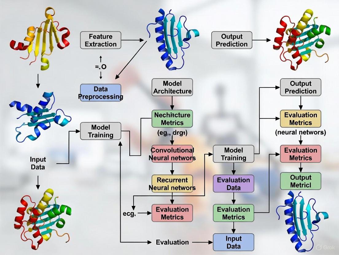
Figure 2: ML Protein Structure Prediction Workflow

Machine Learning Approaches to Structure Prediction

Modern machine learning methods have revolutionized protein structure prediction by replacing traditional energy models and sampling procedures with neural networks [2] [3]. These approaches leverage patterns learned from the Protein Data Bank (PDB) and evolutionary information from multiple sequence alignments to predict structures with remarkable accuracy.

Deep learning systems like AlphaFold2 employ an end-to-end neural network architecture that directly maps from amino acid sequence to atomic coordinates [3]. The key innovation involves the integration of multiple data sources:

• Evolutionary Information: Physical contacts extracted from the evolutionary record through co-evolutionary analysis [2]
• Sequence-Structure Patterns: Patterns distilled from known structures in the PDB [2]
• Template Incorporation: Structural templates from homologs in the Protein Data Bank [2]
• Refinement Procedures: Neural networks that refine coarsely predicted structures into high-resolution models [2]

These approaches have achieved median accuracies of 2.1 Ã… for single protein domains, enabling a fundamental reconfiguration of biomolecular modeling in the life sciences [2] [3].

Research Reagent Solutions for ML-Driven Structural Biology

Table 3: Essential Research Tools for Protein Structure Analysis

Reagent/Resource	Function	Application Context
AlphaFold2/ColabFold	Deep learning structure prediction	Rapid 3D model generation from sequence [4]
trRosetta	Deep residual-convolutional network	Protein structure prediction with distance constraints [4]
DeepMSA	Multiple sequence alignment generation	Enhanced evolutionary constraint detection [4]
Molecular Dynamics Software	Simulation of protein dynamics	Conformational ensemble analysis [4]
Unique Resource Identifiers	Standardized reagent identification	Reproducible experimental protocols [5]

Advanced Applications: Predicting Conformational Ensembles

Proteins exist as dynamic ensembles of multiple conformations rather than single static structures, and these structural changes are often associated with functional states [4]. Recent advances combine machine learning with molecular dynamics simulations to investigate protein conformational landscapes.

Integrated ML/MD Pipeline:

• Distance Distribution Prediction: Use deep learning approaches (e.g., trRosetta) to predict statistical distance distributions between residue pairs from MSA
• Ensemble Generation: Employ distance constraints to generate multiple structural models representing conformational diversity
• Energy Filtering: Filter predicted models based on energy scores from force fields like AWSEM
• Cluster Analysis: Perform RMSD clustering to identify representative conformations
• Validation: Compare predicted ensembles to experimental structures and MD simulations [4]

This integrated approach demonstrates that current state-of-the-art methods can capture experimental structural dynamics, including different functional states observed in crystal structures and conformational sampling from molecular dynamics simulations [4]. The ability to predict multiple biologically relevant conformations has significant implications for drug discovery, as it enables structure-based drug design against different functional states of target proteins.

The hierarchical nature of protein structure—from the linear amino acid sequence to complex multi-subunit assemblies—provides the conceptual framework for understanding protein function and for developing computational prediction methods. Experimental protocols for structure determination yield the foundational data required for training machine learning systems, while biochemical characterization validates computational predictions.

The integration of machine learning with structural biology has created a transformative paradigm in which prediction and experimentation operate synergistically. Deep learning approaches now achieve accuracies that enable reliable structural models for the entire proteome of many organisms, dramatically expanding the structural information available for drug discovery and basic research. As these methods continue to evolve, particularly in predicting conformational ensembles and multi-protein complexes, they will increasingly guide experimental design and accelerate therapeutic development.

The prediction of a protein's three-dimensional structure from its amino acid sequence alone represents one of the most enduring challenges in computational biology. This problem, central to understanding biological function at a molecular level, is framed by two foundational concepts: Anfinsen's dogma and Levinthal's paradox. Christian Anfinsen's Nobel Prize-winning work established that a protein's native structure is determined solely by its amino acid sequence under physiological conditions [6]. This principle suggests that protein structure prediction should be theoretically possible. However, Cyrus Levinthal's subsequent paradox highlighted the computational infeasibility of this task, noting that a random conformational search for even a small protein would take longer than the age of the universe [6] [7].

For decades, these contrasting concepts defined the core challenge of protein folding. The resolution has emerged through sophisticated machine learning approaches that leverage evolutionary information and physical constraints to navigate the vast conformational space efficiently. This document outlines the key theoretical foundations, quantitative benchmarks, and practical protocols for implementing modern protein structure prediction pipelines, with particular emphasis on their application in drug discovery and biomedical research.

Theoretical Foundations and Key Concepts

Anfinsen's Dogma: The Thermodynamic Hypothesis

Anfinsen's dogma, also termed the thermodynamic hypothesis, proposes that the native folded structure of a protein corresponds to its global free energy minimum under physiological conditions [6] [8]. This principle implies that all information required for folding is encoded within the protein's amino acid sequence, making computational structure prediction a theoretically solvable problem. This hypothesis formed the foundational motivation for decades of research in computational protein structure prediction.

Levinthal's Paradox: The Kinetic Challenge

In contrast, Levinthal's paradox highlights the practical impossibility of protein folding via a random conformational search. With an estimated 10³⁰⁰ possible conformations for a typical protein, even sampling at nanosecond rates would require time exceeding the universe's age [7] [6]. Levinthal himself proposed that proteins fold through specific, guided pathways with stable intermediate nucleation points—a concept that aligns with modern funnel-shaped energy landscape theory [7].

Resolution Through Machine Learning

Contemporary deep learning approaches effectively bridge these concepts by learning to identify the native structure (Anfinsen's global minimum) without exhaustively sampling all conformations (solving Levinthal's paradox). These methods leverage evolutionary information from multiple sequence alignments (MSAs) and physical constraints to directly predict plausible low-energy structures [9] [10].

Table 1: Core Concepts in Protein Folding

Concept	Key Principle	Implication for Structure Prediction
Anfinsen's Dogma	Native structure represents the global free energy minimum [6]	Structure is theoretically predictable from sequence alone
Levinthal's Paradox	Random conformational search is kinetically impossible [7]	Requires efficient search strategies to navigate conformational space
Folding Funnel	Guided folding through uneven energy landscape [7]	Provides a conceptual framework for iterative refinement in ML models
Co-evolutionary Constraints	Spatially proximate residues evolve in a correlated manner [9]	Enables contact/distance prediction from multiple sequence alignments

Quantitative Advances in Structure Prediction

Performance Benchmarks in CASP Experiments

The Critical Assessment of protein Structure Prediction (CASP) experiments provide the gold-standard benchmark for evaluating prediction accuracy. The progression of results demonstrates the dramatic improvement enabled by deep learning approaches, particularly AlphaFold2 and its successors.

Table 2: Evolution of Prediction Accuracy in CASP Experiments

CASP Edition (Year)	Leading Method	Median Accuracy (Backbone)	Key Innovation
CASP13 (2018)	AlphaFold (v1)	~3-5 Ã…	Distogram prediction, geometric constraints [10]
CASP14 (2020)	AlphaFold2	0.96 Ã… (r.m.s.d.95)	End-to-end deep learning, Evoformer, structure module [9]
CASP16 (2024)	AlphaFold3	Near-experimental accuracy	Complex prediction (proteins, nucleic acids, ligands) [11] [12]

The accuracy achieved by AlphaFold2 in CASP14—with median backbone accuracy of 0.96 Å (comparable to the width of a carbon atom)—represented a paradigm shift, making predictions competitive with experimental methods in many cases [9]. Subsequent versions have extended these capabilities to molecular complexes.

Key Metrics for Evaluation

• RMSD (Root Mean Square Deviation): Measures the average distance between corresponding atoms in predicted and experimental structures. Lower values indicate better accuracy [9].
• pLDDT (Predicted Local Distance Difference Test): Per-residue confidence score ranging from 0-100, where higher values indicate more reliable predictions [9].
• TM-Score (Template Modeling Score): Global structure similarity measure that is less sensitive to local variations than RMSD [9].

Experimental Protocols for Structure Prediction

End-to-End Prediction with AlphaFold2

Objective: Predict the 3D structure of a protein monomer from its amino acid sequence.

Input Requirements: Amino acid sequence (≥20 residues, ≤2500 residues) in FASTA format.

Procedure:

• Multiple Sequence Alignment Generation

  • Search against major sequence databases (UniRef90, UniRef30, BFD) using HHblits or JackHMMER to generate an MSA [10] [13].
  • For optimal results, use DeepMSA2 to construct deeper alignments by integrating multiple database sources [10].
  • Expected Output: MSA file in A3M or STOCKHOLM format.

• Template Identification (Optional)

  • Search PDB70 database using HHsearch to identify potential structural templates.
  • This step provides additional structural constraints but has minimal impact on final accuracy for most targets [13].

• Model Inference

  • Process inputs through the Evoformer module to generate a pair representation and processed MSA [9].
  • Pass these representations to the structure module that employs an equivariant transformer to iteratively refine atomic coordinates [9] [13].
  • Implement 3 cycles of recycling to iteratively refine predictions [9].
  • Output: Predicted structure in PDB format, per-residue pLDDT confidence scores, and predicted aligned error.

• Model Selection and Validation

  • Select the model with highest predicted confidence (pLDDT).
  • Interpret pLDDT scores: >90 (very high), 70-90 (confident), 50-70 (low), <50 (very low) [9].
  • For low-confidence regions, consider alternative conformations or experimental validation.

Figure 1: AlphaFold2 Protein Structure Prediction Workflow

Template-Free Prediction for Novel Folds

Objective: Predict structures when no homologous templates are available (true de novo prediction).

Input Requirements: Amino acid sequence with no close homologs in PDB.

Procedure:

• Advanced MSA Construction

  • Employ metagenomic sequencing databases (as implemented in DeepMSA) to detect distant evolutionary relationships [10].
  • Use HMM-HMM alignment strategies to capture very remote homology signals.

• Alternative Model Selection

  • Utilize protein language model-based predictors (ESMfold, OmegaFold) that leverage learned sequence representations instead of explicit MSAs [13].
  • These methods trade some accuracy for significantly faster runtimes and can capture structural principles from sequence statistics alone.

• Conformational Sampling

  • For low-confidence predictions, implement aggressive sampling protocols (e.g., AFSample) that generate diverse decoy structures [13].
  • Use AlphaFold2 as an oracle to rank generated decoys by predicted confidence.

• Validation Strategies

  • Compare predictions from multiple independent methods (AlphaFold2, RoseTTAFold, ESMfold).
  • Analyze conserved structural motifs and domain organization for biological plausibility.
  • For critical applications, validate low-confidence regions through targeted mutagenesis experiments.

The Scientist's Toolkit: Essential Research Reagents

Table 3: Key Resources for Protein Structure Prediction Research

Resource	Type	Function	Access
AlphaFold2/3	Software	End-to-end structure prediction from sequence	AlphaFold2: open source; AlphaFold3: academic use only [12]
RoseTTAFold All-Atom	Software	Predict structures of proteins, RNA, DNA and complexes	MIT License (code), non-commercial weights [12]
ColabFold	Software	Faster implementation combining AlphaFold2 and MMseqs2	Open source, free Google Colab access [13]
ESMfold	Software	Protein language model for fast prediction without MSA	Open source [13]
OpenFold	Software	Open-source AlphaFold2 reimplementation with training code	Open source [12] [13]
Boltz-1	Software	Fully open-source alternative to AlphaFold3	Open source, commercial use allowed [12]
PDB (Protein Data Bank)	Database	Experimental structures for training and validation	Free access [10]
UniProt/TrEMBL	Database	Protein sequences for MSA generation	Free access [10]
C.I. Mordant Red 7	C.I. Mordant Red 7|CAS 3618-63-1|Mordant Dye		Bench Chemicals
DBCO-NHCO-PEG4-acid	DBCO-NHCO-PEG4-acid, CAS:1870899-46-9, MF:C32H40N2O9, MW:596.68	Chemical Reagent	Bench Chemicals

Signaling Pathways and Logical Relationships

The core innovation of modern protein structure prediction lies in the integration of evolutionary information with physical constraints through specialized neural network architectures.

Figure 2: Logical Framework Bridging Theory and Implementation

Applications in Drug Discovery and Biomedical Research

The unprecedented accuracy of modern structure prediction tools has transformed their application across biomedical research:

• Drug Target Identification: Rapid structural characterization of potential drug targets, including membrane proteins notoriously difficult to study experimentally [8] [12].
• Mechanism of Action Studies: Understanding disease mutations by mapping them to structural contexts and predicting their disruptive effects [8] [13].
• Antibody Design: Prediction of antibody-antigen complex structures to guide therapeutic antibody engineering [12].
• Small Molecule Docking: Despite limitations in small molecule binding pocket prediction, AlphaFold3 shows improved capability for predicting protein-ligand interactions [12].

For drug discovery pipelines, the recommended workflow involves using open-source alternatives like Boltz-1 or RoseTTAFold for commercial applications, supplemented with experimental validation for critical targets [12].

Future Directions and Protocol Adaptation

The field continues to evolve rapidly, with several emerging trends requiring protocol adaptation:

• Complex Prediction: Move beyond single chains to multi-protein complexes, protein-nucleic acid interactions, and large assemblies [11] [12].
• Conformational Dynamics: Development of methods to predict alternative conformations and folding intermediates, not just static structures [13].
• Integration with Experimental Data: Hybrid approaches that combine computational predictions with sparse experimental data (Cryo-EM, NMR, cross-linking) [10].
• Generative Design: Inversion of the structure prediction problem to design novel protein sequences that fold into desired structures [13].

For research teams, establishing a flexible infrastructure that can incorporate new model architectures as they emerge while maintaining backward compatibility with existing workflows is essential for long-term research productivity.

The field of structural biology is defined by a fundamental and growing asymmetry: the explosive growth in protein sequence data vastly outpaces the slow accumulation of experimentally solved structures. This data gap presents both a significant challenge and a compelling opportunity for research in machine learning-based protein structure prediction.

The core of this disparity is quantified in the data from major biological repositories. The following table illustrates the current scale of this imbalance:

Table 1: The Protein Sequence-Structure Gap as of 2025

Data Type	Repository	Count	Citation
Protein Sequences	UniProtKB/TrEMBL	Over 250 million	[14]
Protein Sequences	UniRef	Over 250 million	[14]
Experimentally Solved Structures	Protein Data Bank (PDB)	~210,000	[14] [15]
General Protein Sequences	TrEMBL Database (2022)	Over 200 million	[16]

This discrepancy exists because high-throughput sequencing technologies can generate protein sequences quickly and inexpensively from genomic data. In contrast, experimental methods for determining protein structures—such as X-ray crystallography, nuclear magnetic resonance (NMR) spectroscopy, and cryo-electron microscopy (cryo-EM)—are often time-consuming, expensive, and technically demanding [15] [17] [16]. The rate at which new protein sequences are discovered has created a massive gap that computational methods, particularly machine learning, are now poised to address.

Successful development of machine learning models for structure prediction relies on a curated set of data resources and software tools. The table below details the essential components of the research toolkit.

Table 2: Essential Research Reagents and Resources for ML-Based Protein Structure Prediction

Category	Resource Name	Primary Function	Key Features/Application
Primary Data Repositories	Protein Data Bank (PDB)	Repository for experimentally determined 3D structures of proteins and nucleic acids.	Source of atomic-level structural data for training and validation; provides annotations for secondary structure and functional sites. [14] [17]
	UniProtKB	Comprehensive protein sequence and functional information database.	Divided into manually curated Swiss-Prot and automatically annotated TrEMBL; essential for sequence-based analysis. [14]
Specialized Databases	DisProt	Manually curated database of Intrinsically Disordered Regions (IDRs).	Provides experimentally validated disorder annotations for benchmarking predictors. [14]
	MobiDB	Resource for intrinsic protein disorder annotations.	Combines experimental and computational annotations for large-scale analyses. [14]
Benchmarking Initiatives	CASP (Critical Assessment of protein Structure Prediction)	Biennial community-wide blind assessment of protein structure prediction methods.	Gold-standard competition for evaluating the accuracy of new prediction tools, including EMA methods. [14] [17] [18]
	CAID (Critical Assessment of Intrinsic Disorder)	Benchmarking initiative for IDR prediction tools.	Uses high-quality datasets from DisProt and PDB to standardize evaluation. [14]
Software Tools & Frameworks	AlphaFold	Deep learning system for highly accurate protein structure prediction.	Uses MSAs and novel neural network architectures (Evoformer) to predict atomic coordinates. [18] [19]
	ESMFold / OmegaFold	Single-sequence-based protein structure predictors.	Leverage protein language models (PLMs) for fast prediction without explicit MSAs. [20]
	SPIRED	Lightweight, single-sequence-based structure prediction model.	Designed for fast inference and integration into end-to-end fitness prediction frameworks. [20]

Machine Learning Approaches to Bridge the Gap

Machine learning, particularly deep learning, has revolutionized protein structure prediction by learning the complex mapping from amino acid sequences to their three-dimensional structures. These approaches can be broadly categorized, each with distinct methodologies for leveraging available data.

Table 3: Categories of Machine Learning Approaches for Protein Structure Prediction

Category	Description	Key Methodologies	Representative Tools
Template-Based Modeling (TBM)	Utilizes known protein structures (templates) as a basis for predicting the structure of a homologous target sequence.	Homology Modeling, Threading (Fold Recognition)	MODELLER [15] [16], SWISS-MODEL [17], HHpred [15]
Template-Free Modeling (TFM)	Predicts structure directly from sequence and MSAs without relying on global template structures. Also includes modern AI-based methods.	Co-evolutionary Analysis (DCA), Deep Learning on MSAs	AlphaFold [18] [19], RoseTTAFold [20], trRosetta [15]
Single-Sequence Prediction	A sub-category of TFM that uses Protein Language Models (PLMs) to predict structure from a single sequence, bypassing the need for explicit MSA construction.	Protein Language Models (PLMs), Transformer Architectures	ESMFold [20], OmegaFold [20], SPIRED [20]
Ab Initio / Free Modeling	Predicts structure based purely on physicochemical principles and energy minimization, without relying on existing structural templates.	Molecular Dynamics, Physics-Based Energy Functions	Rosetta [15] [19], QUARK [15]

End-to-End Prediction and Fitness Workflow

Modern research frameworks are evolving to integrate structure prediction directly with downstream functional analysis, such as predicting the effects of mutations on protein fitness and stability.

Experimental Protocols for Model Training and Validation

Protocol: Building a Supervised Learning Model for Structure Prediction

This protocol outlines the key steps for training a deep learning model to predict protein structures from sequences, using resources like the PDB.

• Dataset Curation and Preprocessing

  • Source Raw Data: Download protein sequences and structures from the PDB. The PDB provides atomic coordinates and curated annotations like secondary structure elements [14].
  • Filter Data: Apply selection criteria such as a minimum resolution (e.g., < 2.5 Ã…) for X-ray structures to ensure high-quality training data [21].
  • Remove Redundancy: Use a filter based on sequence identity (e.g., no pair of sequences in the training set shares >25% identity) to create a non-redundant dataset and minimize data leakage [21].
  • Split Data: Partition the filtered dataset into training, validation, and test sets, ensuring no homologous proteins are shared between sets.

• Feature Engineering and Input Representation

  • Sequence Features: Encode the primary amino acid sequence using one-hot encoding or embeddings from a pre-trained Protein Language Model (PLM) [14] [20].
  • Evolutionary Features: Generate Multiple Sequence Alignments (MSAs) for the target protein using databases like UniRef and the BFD [14] [18]. Process MSAs into position-specific scoring matrices (PSSMs) or profile hidden Markov models [15].
  • Template Information (Optional): For template-based models, identify homologous templates via sequence-sequence or sequence-structure alignment and extract relevant structural features [15] [16].

• Model Architecture and Training

  • Select Architecture: Choose a suitable deep learning architecture. Modern models often use:
    • Evoformer (as in AlphaFold2): A novel architecture that jointly processes MSA and pairwise representations, using attention mechanisms to reason about spatial and evolutionary relationships [18].
    • Graph Neural Networks (GNNs): To operate on the predicted structure for downstream tasks like fitness prediction [20].
  • Define Output and Loss: The output is a 3D structure. The loss function typically combines terms for the frame-aligned point error (FAPE) and violations of physical constraints [18]. Newer models like SPIRED employ a relative displacement loss (RD Loss) to enhance efficiency [20].
  • Train Model: Optimize model parameters on the training set, using the validation set for hyperparameter tuning and to monitor for overfitting.

• Model Validation and Benchmarking

  • Internal Validation: Evaluate the final model on the held-out test set using metrics like TM-score (for global fold accuracy) and lDDT (for local distance-based accuracy) [20].
  • Independent Benchmarking: Assess model performance on independent, time-split datasets (e.g., proteins released after the training data cutoff) and in community-wide blind assessments like CASP or CAMEO to ensure generalizability and state-of-the-art performance [18] [20].

Protocol: End-to-End Prediction of Protein Fitness from Sequence

This protocol describes the workflow for using an integrated model like SPIRED-Fitness to predict mutational effects directly from a single sequence.

• Input Preparation: Provide the wild-type amino acid sequence. Optionally, specify single or double mutations for fitness prediction [20].
• Structure and Feature Extraction: The sequence is passed through the pre-trained SPIRED module, which acts as an information extractor and outputs the predicted 3D structure. The structural information is encoded as a graph or a set of inter-residue relationships [20].
• Fitness Prediction: The structural representation is fed into a downstream graph neural network that has been trained on deep mutational scanning (DMS) data. This network learns to map structural features to fitness scores [20].
• Output and Interpretation: The model outputs a fitness score for the input sequence (and/or its mutants). For stability prediction (SPIRED-Stab), the output is the predicted change in stability (ΔΔG or ΔTm) [20].
• Finetuning (Optional): The entire framework (structure prediction + fitness prediction) can be finetuned end-to-end on specific fitness or stability datasets to improve performance on a particular task [20].

The disparity between billions of protein sequences and only thousands of solved structures is a defining challenge in modern biology. However, as outlined in this application note, the rise of sophisticated machine learning frameworks has created a viable path to bridge this gap. By leveraging curated biological databases, standardized benchmarking practices, and end-to-end deep learning models, researchers can now accurately predict protein structures and their functional consequences at scale. This capability is set to profoundly accelerate research in fundamental biology and streamline the process of drug development.

The evolution of computational methods for protein structure prediction represents a cornerstone of modern structural bioinformatics and a critical foundation for building effective machine learning models. The transformation from early physical principles-based approaches to today's deep learning-powered systems has been marked by key methodological paradigms: homology modeling, threading, and ab initio prediction. These approaches provide the conceptual framework and historical data essential for developing new machine learning algorithms in structural biology. For researchers and drug development professionals, understanding this evolution is not merely academic; it directly informs the selection of appropriate tools, the interpretation of AI model outputs, and the strategic design of novel predictive pipelines. The following application notes and protocols detail the technical specifications, experimental workflows, and practical implementations of these foundational methods within the context of modern machine learning research for protein structure prediction.

Methodological Foundations and Quantitative Comparison

The table below summarizes the core principles, evolutionary context, and performance characteristics of the three primary computational methods for protein structure prediction.

Table 1: Comparative Analysis of Protein Structure Prediction Methods

Method	Core Principle	Evolutionary Context	Accuracy & Limitations	Representative Tools
Homology Modeling (Comparative Modeling)	Predicts structure based on sequence similarity to a protein with a known structure (template) [22] [16] [23].	One of the earliest and most widely used computational techniques; relies on the availability of homologous templates in databases [23].	Accuracy: RMSD of 1-2 Ã… if sequence identity >30% [22]. Limitations: Accuracy declines with decreasing sequence identity; cannot predict novel folds [22] [23].	SWISS-MODEL [22], MODELLER [22], I-TASSER (threading+assembly) [22]
Threading (Fold Recognition)	Fits a target sequence into a library of known structural folds, regardless of sequence similarity [22] [16] [23].	Developed to address the "protein folding problem" when no clear homologous template exists [22] [23].	Use Case: Effective for proteins with low sequence identity but known structural folds [22]. Limitations: Performance depends on the comprehensiveness of the fold library and scoring functions [16].	Phyre2 [22], HHpred [22], I-TASSER (threading+assembly) [22]
Ab Initio (De Novo)	Predicts structure from physical principles and energy minimization without using homologous templates [22] [24] [16].	Represents a fundamentally different approach; computationally demanding but can predict novel folds [23].	Accuracy: Traditionally limited for large proteins; modern variants like C-QUARK show significant improvement (e.g., 75% success rate on test set vs. 29% for earlier QUARK) [25]. Limitations: Extremely computationally intensive [22] [25].	Rosetta [22], QUARK [22], C-QUARK [25]

Experimental Protocols and Workflows

Protocol 1: Homology Modeling with MODELLER

This protocol outlines the standard five-step workflow for building a protein structural model using a known homologous structure as a template [22] [16].

Workflow Diagram: Homology Modeling

Step-by-Step Procedure:

• Template Identification

  • Objective: Identify a suitable protein structure template from the Protein Data Bank (PDB) with significant sequence similarity to the target.
  • Procedure: Perform a sequence search using BLAST or PSI-BLAST against the PDB. A template with a sequence identity of >30% is generally considered suitable for reliable modeling [22] [16].
  • Output: A PDB file of the template and a sequence alignment file.

• Target-Template Alignment

  • Objective: Create an accurate sequence alignment between the target and template sequences.
  • Procedure: Use alignment software (e.g., ClustalOmega, MUSCLE) to align the target sequence with the template sequence. Manually inspect and adjust the alignment, especially in regions of insertions (loops) or deletions.
  • Output: A refined multiple sequence alignment (MSA) file.

• Model Building

  • Objective: Construct a 3D model of the target protein.
  • Procedure: Using a modeling package like MODELLER, copy the backbone coordinates from the template to the target based on the alignment. Model sidechains and any regions not present in the template (e.g., loops) using internal algorithms and fragment libraries [22].
  • Output: A preliminary 3D atomic model in PDB format.

• Model Refinement

  • Objective: Optimize the model's stereochemistry and minimize atomic clashes.
  • Procedure: Subject the initial model to energy minimization using molecular dynamics force fields. This step relaxes the model, correcting unrealistic bond lengths, angles, and van der Waals contacts.
  • Output: An energy-minimized 3D model.

• Model Validation

  • Objective: Assess the quality and reliability of the final model.
  • Procedure: Use tools like PROCHECK to analyze Ramachandran plot outliers, and MolProbity to check for steric clashes and other geometric inconsistencies [23].
  • Output: Validation reports and a quality score for the final model.

Protocol 2: Contact-Assisted Ab Initio Folding with C-QUARK

This protocol details a modern ab initio approach that integrates predicted contact-maps to guide fragment assembly simulations, significantly enhancing accuracy [25].

Workflow Diagram: C-QUARK Ab Initio Folding

Step-by-Step Procedure:

• Input and MSA Generation

  • Objective: Gather evolutionary information from homologous sequences.
  • Procedure: Search whole-genome and metagenome sequence databases (e.g., UniRef) using the target sequence to build a deep Multiple Sequence Alignment (MSA) [25].
  • Output: A comprehensive MSA file.

• Contact-Map Prediction

  • Objective: Predict long-range residue-residue contacts to guide folding.
  • Procedure: Process the MSA through deep-learning and coevolution-based predictors (e.g., DCA) to generate multiple contact-maps. These maps indicate the probability of two residues being spatially close [25].
  • Output: A set of predicted contact-maps with associated confidence scores.

• Fragment Library Assembly

  • Objective: Provide a library of local structural elements as building blocks.
  • Procedure: Extract short (1-20 residues) protein fragments from the PDB that are sequence-similar to local regions of the target. These fragments are used to assemble the full-length model [25].
  • Output: A library of structural fragments.

• Replica-Exchange Monte Carlo (REMC) Simulation

  • Objective: Assemble the full-length structure through conformational sampling.
  • Procedure: Guide the REMC simulation using a composite force field. This field integrates knowledge-based energy terms, fragment-derived contacts, and the sequence-based contact-map predictions via a novel "3-gradient (3G) contact potential". This potential effectively balances the noisy contact information with the physical force field [25].
  • Output: A large ensemble of decoy structures.

• Model Selection and Validation

  • Objective: Identify the most representative and accurate model from the decoy ensemble.
  • Procedure: Cluster all generated decoys using SPICKER. Select the model from the largest and most densely populated cluster as the final prediction [25].
  • Output: A final, clustered 3D model. Accuracy is typically assessed using TM-score (where >0.5 indicates a correct fold) or Global Distance Test (GDT_TS) [25].

Table 2: Key Resources for Computational Protein Structure Prediction

Category	Item / Software	Function in Research	Application Context
Databases	Protein Data Bank (PDB)	Repository of experimentally determined 3D structures of proteins and nucleic acids; essential for template sourcing and model training [22] [16].	All methods, particularly Homology Modeling and Threading.
	UniProt / TrEMBL	Comprehensive protein sequence database; critical for generating Multiple Sequence Alignments (MSAs) [16].	Ab Initio (C-QUARK) and modern deep learning models.
Software & Tools	BLAST / PSI-BLAST	Algorithm for identifying homologous sequences and structures in databases [22] [23].	Homology Modeling (Template Identification).
	MODELLER	Software for building protein 3D models from sequence alignment and template structure [22].	Homology Modeling.
	Rosetta	Suite for biomolecular structure prediction and design; uses fragment assembly and energy minimization [22] [13].	Ab Initio Prediction.
	QUARK / C-QUARK	Ab initio protein structure prediction by replica-exchange Monte Carlo simulation; C-QUARK integrates contact restraints [25].	Ab Initio Prediction.
Validation Services	PROCHECK / MolProbity	Tools for stereochemical quality assessment of protein structures (e.g., Ramachandran plots) [23].	Model validation across all methods.
Computational Infrastructure	High-Performance Computing (HPC) Cluster	Essential for running computationally intensive simulations like REMC in ab initio methods [22] [25].	Ab Initio Prediction, large-scale analysis.

Integration with Machine Learning Research

The evolution from classical methods to modern machine learning models like AlphaFold2 is a continuum of increasing abstraction and integration. AlphaFold2's architecture implicitly incorporates principles from all three historical methods. Its Evoformer module processes MSAs to extract co-evolutionary signals, a concept central to both threading and contact-assisted ab initio folding [13]. The structure module then performs a geometric construction of the atomic coordinates, analogous to a highly optimized and informed model-building step [13].

For researchers building new machine learning models, this history provides critical insights. The success of C-QUARK demonstrates that even low-accuracy contact predictions, when intelligently integrated with physical simulation (3G potential), can dramatically improve outcomes [25]. This suggests hybrid approaches that combine deep learning predictions with physics-based refinement remain a powerful strategy. Furthermore, the limitations of these classical methods—such as homology modeling's reliance on templates and ab initio's computational cost—define the very problems that machine learning models must solve to generalize effectively. Understanding the specific failure modes and success metrics (e.g., TM-score, GDT_TS) of these established protocols is crucial for benchmarking and validating new AI-driven approaches.

For over 50 years, the "protein folding problem"—predicting a protein's three-dimensional structure from its amino acid sequence—stood as a grand challenge in biology [26]. Understanding protein structure is fundamental to elucidating biological function and accelerating drug discovery. Traditional experimental methods like X-ray crystallography and cryo-electron microscopy are time-consuming and expensive, creating a massive gap between known protein sequences and solved structures [27] [28]. While computational approaches existed, they fell far short of atomic accuracy, especially when no homologous structure was available [26]. This document provides application notes and experimental protocols for building machine learning models that transformed this field, enabling rapid, accurate protein structure prediction.

Quantitative Breakthrough: Performance Metrics Before and After Deep Learning

The Critical Assessment of protein Structure Prediction (CASP) serves as the gold-standard blind assessment for evaluating prediction accuracy [26]. The performance leap enabled by deep learning is quantitatively demonstrated below.

Table 1: Key Performance Metrics at CASP14 for AlphaFold2 and Next Best Method

Metric	AlphaFold2	Next Best Method	Improvement Factor
Median Backbone Accuracy (Cα RMSD95)	0.96 Å	2.8 Å	~2.9x
All-Atom Accuracy (RMSD95)	1.5 Ã…	3.5 Ã…	~2.3x
Comparative Accuracy	Competitive with experimental structures in most cases	Far short of experimental accuracy	Revolutionary

Abbreviations: RMSD95, Root-mean-square deviation at 95% residue coverage; Cα, Alpha carbon [26].

Table 2: Comparative Analysis of Major Protein Structure Prediction Methods

Method	Category	Key Principle	Representative Tool
Homology Modeling	Template-Based Modeling (TBM)	Uses a closely related homologous protein as a structural template [27].	SWISS-MODEL [28]
Threading/Fold Recognition	Template-Based Modeling (TBM)	Fits sequence into a known structural fold, even with low sequence similarity [27] [28].	GenTHREADER [28]
Ab Initio	Free Modeling (FM)	Relies on physicochemical principles and energy minimization without templates [27] [28].	QUARK [28]
Deep Learning (AlphaFold2)	Free Modeling (FM)	Uses neural networks to learn evolutionary, physical, and geometric constraints from data [26].	AlphaFold2 [26]

Experimental Protocols for Deep Learning-Based Structure Prediction

Protocol 1: Implementing an AlphaFold2-Style Architecture

This protocol outlines the core architectural components and training procedure for a state-of-the-art prediction model, based on the AlphaFold2 system [26].

I. Input Representation and Feature Engineering

• A. Multiple Sequence Alignment (MSA) Construction: Input the target amino acid sequence. Use a tool like HHblits to search large genomic databases (e.g., UniRef, BFD) to generate a Multiple Sequence Alignment (MSA). The MSA represents the evolutionary history of the protein and is formatted as an ( N{seq} \times N{res} ) array, where ( N{seq} ) is the number of homologous sequences and ( N{res} ) is the number of residues [26].
• B. Pair Representation Generation: Compute an ( N{res} \times N{res} ) array representing potential residue-pair interactions. This matrix is initialized from the MSA and may incorporate other features like co-evolutionary signals and template information if available [26].

II. Neural Network Architecture: The Evoformer and Structure Module

• A. Evoformer Processing (Trunk): The Evoformer is a novel neural network block designed to process the inputs [26].
  • Pass the MSA and pair representations through a stack of Evoformer blocks.
  • Within each block, use attention mechanisms and triangle multiplicative updates to allow continuous information exchange between the MSA and pair representations, enforcing spatial and evolutionary constraints [26].
  • The output is a "processed" MSA and a refined pair representation that contains a concrete structural hypothesis.

• B. Structure Module: This module translates the abstract representations into explicit 3D atomic coordinates [26].
  • Initialize a set of residue-level rigid body frames (rotations and translations) in a trivial state.
  • Process these frames through an equivariant attention architecture, which respects the geometric symmetries of 3D space.
  • The network implicitly reasons about all atoms, outputting precise 3D coordinates for all heavy atoms.
  • Use a loss function that heavily weights the orientational correctness of the residues.

III. Training and Iterative Refinement

• A. Recycling: To improve accuracy, the outputs of the entire network (both coordinates and representations) are recursively fed back into the input of the same network modules for several cycles (typically 3-4). This iterative refinement is crucial for high accuracy [26].
• B. Loss Functions: Employ a composite loss function during training:
  • Frame-Aligned Point Error (FAPE): Measures the local structural accuracy.
  • Distogram Loss: Penalizes errors in predicted inter-residue distances.
  • Masked MSA Loss: Helps the model learn meaningful representations by predicting masked portions of the input MSA [26].

Protocol 2: End-to-End Workflow for Prediction and Validation

This protocol describes the complete process from sequence input to model validation, applicable for research and drug discovery pipelines.

I. Data Curation and Pre-processing

• A. Input Sequence Preparation: Obtain the canonical amino acid sequence of the target protein from a reliable database like UniProt. Ensure the sequence is correct and of adequate length.
• B. Database Searching: Configure and run the MSA generation tool (e.g., HHblits, Jackhmmer) against standard databases. This step is computationally intensive and may require high-performance computing (HPC) clusters. Monitor for depth and quality of the MSA.

II. Model Inference and Execution

• A. System Configuration: Run the prediction model (e.g., AlphaFold2, RoseTTAFold) on a system with adequate resources, typically high-end GPUs (e.g., NVIDIA A100, V100) and sufficient RAM (>64 GB recommended).
• B. Execution: Execute the model with the pre-processed MSA and pair features as input. The runtime can vary from minutes for short proteins to hours for very long complexes.

III. Post-processing and Model Validation

• A. Confidence Scoring: The model outputs a per-residue confidence score, the predicted Local Distance Difference Test (pLDDT). This score reliably estimates the local accuracy of the prediction [26]. Visualize the model colored by pLDDT to identify low-confidence regions.
• B. Model Quality Assessment: Calculate global metrics like Template Modeling Score (TM-score) to assess the global fold correctness. A TM-score >0.5 suggests a correct fold, while >0.8 indicates a high-quality model.
• C. Structural Analysis: Use molecular visualization software (e.g., PyMOL, ChimeraX) to manually inspect the predicted structure for plausible stereochemistry, bond lengths, and side-chain packing.

Table 3: Key Research Reagent Solutions for Protein Structure Prediction

Reagent / Resource	Type	Function and Application
Protein Data Bank (PDB)	Database	A worldwide repository of experimentally determined 3D structures of proteins, used for training deep learning models and as templates in TBM [27] [28].
UniProtKB	Database	A comprehensive resource for protein sequence and functional information, used as the primary source for input sequences and for building MSAs [28].
Multiple Sequence Alignment (MSA) Tools	Software	Programs like HHblits and Jackhmmer. They find homologous sequences in genomic databases, providing the evolutionary data that is the primary input for models like AlphaFold2 [26].
AlphaFold Protein Structure Database	Database	A public database providing pre-computed AlphaFold2 predictions for over 200 million proteins, enabling rapid access to models without local computation [29].
RoseTTAFold	Software	An end-to-end deep learning protein structure prediction method, based on a three-track neural network architecture that simultaneously considers sequence, distance, and coordinate information [29].
pLDDT	Metric	The predicted Local Distance Difference Test. A per-residue confidence score provided by AlphaFold2 that estimates the reliability of the local structural prediction [26].

Architectures, Data Pipelines, and Hands-On Implementation

The development of robust machine learning (ML) models for protein structure prediction hinges on access to large-scale, high-quality structural and sequence data. Four data resources form the cornerstone of this research: the Protein Data Bank (PDB), a repository of experimentally determined structures; UniProt, a comprehensive knowledgebase of protein sequences and functional information; the AlphaFold Protein Structure Database, providing expansive access to AI-predicted structures; and the ESM Metagenomic Atlas, which offers structure predictions for metagenomic proteins. For ML practitioners, these resources provide the essential training data, ground truth labels, and benchmarking standards required to develop and validate novel algorithms. The integration of experimental and computationally predicted structures, as showcased in Table 1, enables a multi-faceted approach to model training, addressing the limitations of structural coverage in the experimental data alone.

Table 1: Core Data Sources for Protein Structure Prediction ML Research

Resource	Primary Content	Key Utility for ML	Scale (Approx.)
PDB [30]	Experimentally determined 3D structures (X-ray, NMR, Cryo-EM)	Source of high-accuracy ground truth data for model training and validation	~200,000 structures [9]
UniProt [31]	Manually curated (Swiss-Prot) and automatically annotated (TrEMBL) protein sequences	Provides sequences, functional annotations, and evolutionary context for model input	Millions of sequences [31]
AlphaFold DB [32]	AI-predicted structures for sequences in UniProt	Expands structural coverage for training; provides confident predictions for proteins with unknown structures	Over 200 million entries [32]
ESM Metagenomic Atlas [33] [34]	Structures predicted by ESMFold for metagenomic sequences	Enables exploration of uncharted protein space; trains/fine-tunes models on diverse, novel folds	Over 700 million predicted structures [34]

Resource-Specific Application Notes and Protocols

Protein Data Bank (PDB)

The PDB is the global archive for experimentally determined three-dimensional structures of biological macromolecules, serving as the primary source of structural truth. For ML research, it is critical to parse these files into a structured data format that can be consumed by computational models. The Biopython PDB module provides a robust toolkit for this task, implementing a Structure/Model/Chain/Residue/Atom (SMCRA) architecture to hierarchically organize structural data [35]. This overcomes the limitations of the legacy PDB file format, which has been superseded by the more extensible PDBx/mmCIF format as the standard archive format.

Protocol 2.1.1: Parsing a PDB Structure for Feature Extraction

• Initialize the PDB Parser: Create a PDBParser object. Setting PERMISSIVE=1 allows the parser to tolerate common minor errors in PDB files without failing.

• Load the Structure File: Use the parser to read the PDB file and create a Structure object. The structure_id is a user-defined identifier.

• Extract Atomic Coordinates: Traverse the SMCRA hierarchy to access atomic-level data, such as 3D coordinates.

• Extract Experimental Metadata (Optional): Access information from the PDB file header, though caution is advised as this data can be incomplete. The mmCIF format is more reliable for header information.

For programmatic analysis of the broader PDB, the RCSB PDB API provides structured access to search and retrieve metadata and annotations at scale, which is essential for building large, curated training datasets [30].

UniProt

UniProt is the central hub for protein sequence and functional annotation. For ML, it provides the primary input sequences for structure prediction and the functional labels necessary for developing models that predict biological activity. The UniProt Knowledgebase is divided into Swiss-Prot (manually curated) and TrEMBL (automatically annotated), offering a balance of quality and scale [31]. A key ML application is using the Gene Ontology (GO) terms from UniProt to train models for protein function prediction from sequence or structure.

Protocol 2.2.1: Mapping Protein Sequences to Structures via UniProt

This protocol is critical for creating a high-quality dataset where each sequence is paired with its experimentally determined structure.

• Acquire Sequence and Annotation Data: Download the UniProt dataset in a structured format (e.g., XML, TAB) for the organism of interest via the UniProt website or FTP server.

• Identify Sequences with Structural Data: Filter the dataset using the cross-reference to the PDB. This information is contained in the database(PDB) field in UniProt flat files or the dbreference attribute in XML.

• Resolve Mapping at the Residue Level: For precise modeling, utilize the residue-level mapping between UniProt sequences and PDB structures that is maintained in collaboration with the Macromolecular Structure Database (MSD) group at the EBI [31]. This ensures accurate alignment of sequence positions to structural coordinates, which is vital for tasks like predicting the functional impact of mutations.

• Construct Final Dataset: For each entry in the filtered list, pair the UniProt sequence with the 3D coordinates from the corresponding PDB file, which can be parsed using the methods in Protocol 2.1.1.

AlphaFold DB

AlphaFold DB provides open access to the groundbreaking predictions of AlphaFold 2, a deep learning system that regularly predicts protein structures with accuracy competitive with experiment [32] [9]. For ML research, this database is transformative. It provides predicted structures for the entire human proteome and over 200 million other proteins, massively expanding the structural coverage of known sequences [32]. This allows researchers to train models on a much broader set of protein folds and families than would be possible with experimental data alone. Furthermore, the per-residue confidence metric, the predicted Local Distance Difference Test (pLDDT), allows for the filtering of high-confidence predictions to create reliable training subsets or to identify potentially disordered regions [9].

Protocol 2.3.1: Benchmarking a Custom Model Against AlphaFold DB

This protocol outlines how to use AlphaFold DB predictions as a baseline to evaluate the performance of a novel structure prediction model.

• Define a Test Set: Select a set of protein sequences for which high-quality AlphaFold DB predictions are available. A robust test set should include proteins with diverse folds and lengths.

• Download AlphaFold DB Structures: For each protein in the test set, retrieve the predicted structure and the associated pLDDT scores from the AlphaFold DB website (https://alphafold.ebi.ac.uk).

• Generate Custom Predictions: Run your custom ML model on the same set of protein sequences.

• Calculate Structural Accuracy Metrics: For each protein, compute standard metrics to compare your model's output to the AlphaFold DB prediction.

  • RMSD (Root Mean Square Deviation): Measures the average distance between atoms after structural alignment. Lower values indicate better accuracy. Useful for comparing structures of the same protein.
  • TM-score (Template Modeling Score): A length-independent metric for assessing the topological similarity of protein structures. A score >0.5 suggests generally the same fold, while >0.8 indicates a highly similar fold [36].

• Analyze by Confidence and Length: Stratify the results based on the AlphaFold pLDDT confidence and loop length, as accuracy is known to correlate with these factors. For example, benchmark results should be reported separately for high-confidence (pLDDT > 90) regions versus low-confidence (pLDDT < 70) regions and for short loops (<10 residues) versus long loops (>20 residues), as the latter show lower prediction accuracy (average RMSD of 2.04 Ã…) [36].

ESM Metagenomic Atlas

The ESM Metagenomic Atlas is a repository of over 700 million protein structure predictions generated by ESMFold, a language model-based structure prediction tool [33] [34]. Unlike AlphaFold 2, which relies on co-evolutionary information from multiple sequence alignments (MSAs), ESMFold predicts structure end-to-end directly from a single sequence using a protein language model (ESM-2) that has learned evolutionary patterns from a vast corpus of sequences. This makes it exceptionally fast and well-suited for metagenomic proteins, which often lack homologous sequences for MSA construction [34]. For ML research, this atlas is a treasure trove of novel protein folds from under-explored biological niches, providing unique data for training models to generalize beyond the well-characterized regions of protein space.

Protocol 2.4.1: Using the ESM Atlas API for High-Throughput Data Retrieval

This protocol enables the programmatic downloading of ESMFold structures for large-scale ML training pipelines.

• Install Required Libraries: Ensure you have the requests library installed in your Python environment.

• Construct API Call: Use the ESM Atlas API to submit a protein sequence and receive the predicted structure in PDB format.

• Handle Response and Save Structure: Check for a successful response and save the returned PDB data to a file.

For bulk analysis, the ESMFold model can also be run locally or via ColabFold to generate predictions for custom sequence lists not already in the atlas [33].

Table 2: Key Software Tools and Data Resources

Tool/Resource Name	Type	Primary Function in Research
Biopython PDB Module [35]	Software Library	Parsing PDB, mmCIF, and MMTF files into Python data structures for analysis and feature extraction.
MMCIF2Dict [35]	Software Tool	Creating a Python dictionary from an mmCIF file for low-level access to all data fields.
Mol* [30]	Visualization Software	Interactive 3D visualization and analysis of molecular structures within the RCSB PDB website or as a standalone tool.
ColabFold [34]	Software Suite	Provides accelerated, publicly accessible implementations of AlphaFold2 and ESMFold via Google Colab.
OpenFold [13]	Software Framework	A trainable, open-source reimplementation of AlphaFold2, enabling model introspection and custom training.
Foldseek [34]	Software Suite	Fast, efficient structural similarity search against massive databases like the AFDB or ESM Atlas.

Integrated Workflow for ML Model Development

The true power of these resources is realized when they are integrated into a cohesive workflow for training and validating ML models for structure prediction. The diagram below illustrates a typical pipeline that leverages the unique strengths of each data source.

Diagram 1: Integrated ML workflow for protein structure prediction, showing how core data sources feed into model development and validation.

This workflow begins with Data Curation, where sequences from UniProt are paired with structural data from the PDB (for ground truth), AlphaFold DB (for expanded training set coverage and baseline comparison), and the ESM Metagenomic Atlas (to incorporate novel folds). During Feature Extraction, inputs for the model are prepared, which can include the raw amino acid sequence, computed multiple sequence alignments, and/or embeddings from protein language models like ESM-2. The ML Model Training phase uses these features to learn the mapping from sequence to structure. Frameworks like OpenFold are crucial here, as they are not just for inference but are designed to be retrained, allowing researchers to test new architectures or training strategies [13]. Finally, rigorous Model Validation is performed against held-out experimental structures from the PDB and benchmarked against state-of-the-art predictions from AlphaFold DB and ESMFold to quantify performance improvements.

In the pursuit of building effective machine learning models for protein structure prediction, the representation of amino acid sequences stands as a foundational and critical first step. The chosen representation directly influences a model's ability to capture the complex biochemical principles and evolutionary patterns that govern how a linear sequence of amino acids folds into a three-dimensional structure. The field has evolved significantly from simple, hand-crafted encodings to sophisticated, learnable representations derived from massive sequence databases. Within the context of a protein structure prediction research pipeline, selecting an appropriate sequence encoding method involves balancing computational efficiency, dependency on external data, and the capacity to capture long-range interactions and structural constraints. This protocol outlines the primary sequence representation approaches, their implementation details, and their integration into a complete structure prediction workflow, providing researchers with practical guidance for selecting and applying these methods effectively.

Foundational Sequence Encoding Methods

One-Hot Encoding

One-hot encoding represents each of the 20 standard amino acids in a protein sequence as a binary vector of length 20, where a single element is 1 (indicating the presence of that specific amino acid) and all other elements are 0 [37] [38]. This method treats each amino acid as an independent category without inherent relationships.

Protocol: Implementation of One-Hot Encoding

• Sequence Alignment and Padding: For a dataset of protein sequences, first determine the maximum sequence length (L). Shorter sequences must be padded to this length using a designated null character.
• Dictionary Creation: Create a dictionary mapping each of the 20 amino acid characters (e.g., 'A' for Alanine, 'R' for Arginine) to an integer index from 0 to 19. Include an additional index (e.g., 20) for the padding character.
• Vectorization: For each sequence, convert it into an integer array of length L using the mapping dictionary.
• Binarization: Apply a one-hot encoding function to this integer array. This results in a 2D matrix of size L x 21 (20 amino acids + 1 padding character). The final representation for a batch of sequences is a 3D tensor of shape (Batch Size, L, 21).

Physicochemical and Chemical Feature Encodings

These encodings move beyond categorical identity to represent amino acids by their biochemical properties, such as hydrophobicity, volume, charge, and polarity [38] [39]. More advanced chemical encodings use molecular fingerprints to describe the structure of amino acid side chains.

Protocol: Generating Molecular Fingerprint-Based Encodings

• Fingerprint Generation: For each amino acid, generate a molecular graph with atoms as nodes and chemical bonds as edges. Compute a molecular fingerprint, such as a Morgan fingerprint (circular fingerprint) or an atom-pair fingerprint, which encodes molecular substructures into a fixed-length bit vector [38].
• Dimensionality Reduction: The initial fingerprint vectors are often very high-dimensional (e.g., 4096 bits for Morgan fingerprints). Use the FastMap dimensionality reduction algorithm to project these vectors into a lower-dimensional space (e.g., 14-18 dimensions) while preserving the chemical distances between different amino acids [38].
• Sequence Representation: A protein sequence is represented as a matrix of size L x D, where D is the dimension of the reduced chemical encoding for each amino acid at each position.

Table 1: Comparison of Foundational Sequence Encoding Methods

Encoding Method	Dimensionality per Residue	Key Features	Advantages	Limitations
One-Hot Encoding	20 (or 21 with padding)	Categorical, local information	Simple, interpretable, no external data needed	Does not capture biochemical similarities, high-dimensional sparse matrix
Physicochemical Properties	~7-15 continuous values	Hand-crafted features based on experiments	Encodes known biochemical priors	Limited to pre-defined features, may miss complex patterns
Chemical Fingerprints	~14-18 continuous values	Based on molecular graph structure of side chains	Captures complex chemical relationships	Requires cheminformatics tools, reduction step needed

Advanced Embeddings from Protein Language Models (PLMs)

Protein Language Models (PLMs), inspired by breakthroughs in natural language processing (NLP), learn contextual representations of amino acids by training on millions of diverse protein sequences [40] [41]. They learn the "language" of evolution, capturing complex statistical patterns that reflect structural and functional constraints.

Model Architectures and Training Objectives

• Masked Language Models (e.g., ESM, BERT-style): These models are trained by randomly masking (hiding) portions of the input sequence and then learning to predict the masked tokens based on the full context provided by the unmasked parts of the sequence [37] [41]. This bidirectional context allows the model to learn rich, contextual representations for every position in a sequence. Models like ESM (Evolutionary Scale Modeling) are exemplary implementations of this approach [37].
• Autoregressive Language Models (e.g., UniRep, GPT-style): These models are trained to predict the next amino acid in a sequence given all previous amino acids [37] [41]. While they can capture long-range dependencies, the representation at each position is based only on the preceding context. UniRep is a prominent example that uses a recurrent architecture (mLSTM) for this purpose [37].

Protocol: Generating Embeddings with Pre-trained PLMs

• Model Selection: Choose a pre-trained PLM suitable for your task. Common choices include the ESM family of models (e.g., ESM-2) or UniRep. Ensure the model is compatible with your computational framework (e.g., PyTorch, Hugging Face Transformers).
• Sequence Preparation: Format your input sequences as standard amino acid strings. There is no need for multiple sequence alignment (MSA).
• Embedding Extraction: Pass the sequences through the pre-trained model.
  • For per-residue embeddings, extract the hidden state representations from the final (or an intermediate) layer of the model for each amino acid position. The output is a matrix of size L x E, where E is the embedding dimension (e.g., 1280 for ESM-2).
  • For a global sequence representation, common strategies include computing the mean of all per-residue embeddings or using the embedding of a special token (e.g., [CLS] in BERT-style models). However, research indicates that learning the aggregation via a bottleneck autoencoder can be superior to simple averaging [42].

Ensemble and Hybrid Representation Approaches

Combining multiple representation methods can synergize their strengths and lead to improved predictive performance [37] [38]. An ensemble approach can compensate for the weaknesses of a single method.

Protocol: Creating an Ensemble Representation

• Multiple Encoding Generation: For a given set of sequences, generate multiple independent representations (e.g., One-Hot, ESM embeddings, and fingerprint-based encodings).
• Feature Concatenation: For each sequence, concatenate the different representation vectors (either at the per-residue or global sequence level) into a single, high-dimensional feature vector.
• Model Training: Train a downstream predictor (e.g., a neural network) on this concatenated feature set. The model will learn to weight the importance of the different representations automatically. Studies have shown such ensembles can increase predictive performance for tasks like fitness prediction [37].

Table 2: Overview of Advanced Protein Language Model Embeddings

PLM (Example)	Training Objective	Architecture	Context	Typical Embedding Dimension (E)
ESM (e.g., ESM-2)	Masked Language Modeling	Transformer	Bidirectional (Full)	512 to 1280+
UniRep	Next Token Prediction	mLSTM (Recurrent)	Left-to-right	1900
ProtTrans	Masked Language Modeling	Transformer	Bidirectional (Full)	1024 to 4096

Integration and Practical Workflow for Structure Prediction

Integrating these representations into a structure prediction pipeline requires careful consideration of the task and available resources.

Protocol: A Practical Workflow for Representation Selection

• Problem Scoping:
  • For single-sequence prediction where no homologous sequences are available or computational speed is critical, start with One-Hot encodings or a single-sequence PLM like ESM [38].
  • For maximum accuracy and where external data resources are available, leverage PLM embeddings or profile-based methods that use multiple sequence alignments (MSAs).
• Data Preprocessing: Implement the encoding protocol from Sections 2 or 3 to convert your raw FASTA sequences into numerical tensors.
• Downstream Model Configuration:
  • The architecture of the downstream predictor (e.g., CNN, LSTM, Transformer) should be chosen based on the prediction task (e.g., secondary vs. tertiary structure).
  • When using fixed pre-trained embeddings (i.e., without fine-tuning), the downstream model should be trained to map from the embedding space to the target (e.g., structural class, 3D coordinates). Freezing the embeddings prevents overfitting, especially with limited labeled data [42].
• Handling Imbalanced Data: In protein engineering datasets, high-fitness variants are often rare. Employ sampling techniques like SMOTE (Synthetic Minority Over-sampling Technique) on the sequence representations before training the predictor to improve model performance on minority classes [37].

The Scientist's Toolkit: Research Reagent Solutions

Table 3: Essential Resources for Protein Sequence Representation and Structure Prediction

Resource Name / Category	Function / Purpose	Example Tools / Databases
Pre-trained Protein Language Models	Provide state-of-the-art sequence embeddings for transfer learning without training from scratch.	ESM (Evolutionary Scale Modeling), UniRep, ProtTrans
Molecular Fingerprint Toolkits	Generate chemical feature encodings for amino acid side chains.	RDKit, Open Babel
Protein Sequence Databases	Source of sequences for training new PLMs or for generating multiple sequence alignments (MSAs).	UniProt, Pfam
Protein Structure Databases	Provide ground truth 3D structures for training and benchmarking structure prediction models.	PDB (Protein Data Bank), ProteinNet
Deep Learning Frameworks	Implement, train, and deploy neural network models for structure prediction.	PyTorch, TensorFlow, JAX
303052-45-1	303052-45-1, CAS:303052-45-1, MF:C₁₈₉H₂₈₄N₅₄O₅₈S, MW:4272.70	Chemical Reagent
Urea perchlorate	Urea Perchlorate|High-Purity Research Chemical	Urea perchlorate is a versatile oxidizer for explosives and materials science research. This product is For Research Use Only (RUO). Not for personal use.

Workflow Visualization

The following diagram illustrates the logical workflow for selecting and applying sequence representation methods within a protein structure prediction project.

Deep learning has revolutionized the field of computational biology, providing unprecedented capabilities for predicting protein structures from amino acid sequences. The accurate prediction of protein three-dimensional structures is a cornerstone of modern drug discovery and biological research, enabling scientists to understand disease mechanisms, design novel therapeutics, and explore fundamental biological processes. Among the diverse deep learning architectures available, CNNs, RNNs, and Transformers have emerged as particularly powerful tools, each bringing unique strengths to different aspects of the protein structure prediction pipeline. This article provides detailed application notes and experimental protocols for implementing these core architectures within the context of protein structure prediction research, offering researchers and drug development professionals practical guidance for building effective machine learning models in this rapidly advancing field.

Architectural Strengths and Applications

The three fundamental deep learning architectures—CNNs, RNNs, and Transformers—each process information through distinct mechanistic pathways, making them differentially suited for specific aspects of protein structure prediction.

Convolutional Neural Networks (CNNs) employ hierarchical filters that scan local regions of input data, making them exceptionally well-suited for identifying conserved motifs and local structural patterns in protein sequences. Their translation invariance property allows them to recognize features regardless of their position in the sequence, which is particularly valuable for detecting domain-specific signatures that may recur across different protein families. CNNs typically process data through multiple convolutional layers followed by pooling operations, progressively building more abstract representations of protein features.

Recurrent Neural Networks (RNNs) process sequential data through time-step connections that maintain a hidden state, effectively capturing temporal dependencies in amino acid sequences. Their gated variants, particularly Long Short-Term Memory (LSTM) and Gated Recurrent Unit (GRU) networks, can learn long-range interactions between residues that are spatially distant in the sequence but may be critical for proper folding. This architectural characteristic makes RNNs valuable for modeling the dynamic process of protein folding and capturing non-local contact information.

Transformer architectures utilize self-attention mechanisms to weigh the importance of different residues in relation to each other, enabling them to capture global dependencies across entire protein sequences regardless of distance. This capability is particularly crucial for protein structure prediction, where residues far apart in the linear sequence often come into close proximity in the folded three-dimensional structure. The pre-training of transformer models on massive protein sequence databases has proven exceptionally powerful for learning fundamental principles of protein biochemistry and structural organization.

Quantitative Performance Comparison

Table 1: Performance Comparison of Core Architectures on Protein Structure Prediction Tasks

Architecture	Primary Strength	Optimal Task Application	Training Efficiency	Key Limitation
CNN	Local pattern detection	Secondary structure prediction, residue contact maps	High (parallel processing)	Limited long-range dependency modeling
RNN/LSTM	Sequential dependency modeling	Contact order prediction, folding pathway analysis	Moderate (sequential processing)	Gradient vanishing/explosion in long sequences
Transformer	Global context understanding	Tertiary structure prediction, MSA processing	Variable (high with pre-training)	Computational intensity for very long sequences

The performance characteristics outlined in Table 1 demonstrate how each architecture contributes uniquely to the protein structure prediction pipeline. In practice, state-of-the-art systems like AlphaFold2 and RoseTTAFold often employ hybrid approaches that strategically combine these architectural elements to leverage their complementary strengths [27] [13].

Application Notes and Experimental Protocols

Implementation Framework Setup

Research Reagent Solutions and Essential Materials

Table 2: Essential Research Reagents and Computational Tools

Category	Specific Tool/Library	Function	Implementation Example
Specialized Libraries	DeepProtein	Comprehensive benchmarking and model deployment	Provides unified interface for CNN, RNN, Transformer models across multiple protein tasks [43] [44]
Structure Prediction	ColabFold	Optimized AlphaFold2 implementation	Enables folding of sequences up to 1000 residues with minimal computational requirements [13]
Language Models	ESM-2, ProtT5	Protein sequence representation learning	Generates contextual embeddings from amino acid sequences for downstream prediction tasks [43] [13]
Deployment Platforms	BentoML, TorchServe	Model packaging and serving	Enables production deployment of trained models as scalable APIs [45] [46]

Protocol 1: Initial Framework Configuration

• Environment Setup: Initialize a conda environment with Python 3.9 and install core dependencies including PyTorch 2.1+, DeepPurpose, and Transformers libraries following the DeepProtein installation guidelines [43].

• Hardware Configuration: Configure GPU acceleration with CUDA 11.8 for optimal performance with transformer architectures, which significantly benefit from parallel processing capabilities.

• Data Acquisition: Download and preprocess standard benchmark datasets such as Beta-lactamase for property prediction, SubCellular for localization, and IEDB for protein-protein interaction studies [43].

Architecture-Specific Implementation Protocols

Protocol 2: CNN Implementation for Local Structure Prediction

CNNs excel at identifying local structural motifs and patterns in protein sequences, making them ideal for tasks such as secondary structure prediction and residue contact estimation.

Experimental Workflow:

• Input Representation: Convert amino acid sequences to numerical embeddings using one-hot encoding or pretrained residue representations.

• Architecture Configuration: Implement a multi-scale CNN with kernel sizes of 3, 5, and 7 to capture short, medium, and long-range local patterns within the protein sequence.

• Training Configuration: Set batch size to 32, learning rate to 0.0001, and use Adam optimizer with default parameters as recommended in DeepProtein benchmarks [43].

CNN Multi-Scale Feature Extraction Workflow

Protocol 3: RNN Implementation for Sequential Dependency Modeling

RNNs and their variants are particularly effective for capturing sequential dependencies in protein folding pathways and temporal dynamics.

Experimental Workflow:

• Sequence Preparation: Pad or truncate protein sequences to consistent lengths while preserving positional information through appropriate masking.

• Architecture Selection: Implement a bidirectional LSTM network with 2 layers and 512 hidden units to capture both forward and backward dependencies in the amino acid sequence.

• Regularization Strategy: Apply dropout of 0.2 between LSTM layers and use gradient clipping at 5.0 to mitigate the vanishing/exploding gradient problem common in RNNs.

Protocol 4: Transformer Implementation for Global Context Modeling

Transformers have demonstrated remarkable performance in protein structure prediction through their ability to capture global dependencies using self-attention mechanisms.

Experimental Workflow:

• Input Processing: Generate multiple sequence alignments (MSAs) for target proteins or use pretrained protein language model embeddings from ESM-2 or ProtT5.

• Attention Mechanism: Implement multi-head self-attention with 8-16 heads to enable the model to jointly attend to information from different representation subspaces at different positions.

• Pre-training Utilization: Initialize with pretrained weights from protein language models (ESM, ProtBert) and fine-tune on specific structure prediction tasks, significantly reducing training time and improving accuracy [13].

Transformer Architecture with Residual Connections

Integrated Architecture Implementation

Hybrid Model Protocol

Protocol 5: Implementing a CNN-Transformer Hybrid Architecture

Modern protein structure prediction pipelines increasingly leverage hybrid architectures that combine the strengths of multiple approaches.

Experimental Workflow:

• Local Feature Extraction: Process raw amino acid sequences through CNN layers to capture local motifs and residue neighborhood patterns.

• Global Context Integration: Pass CNN outputs to transformer encoder layers to model long-range dependencies and global sequence context.

• Structure Decoding: Use the combined representation to predict 3D coordinates through a structure module that iteratively refines atomic positions.

• Training Configuration: Employ a multi-stage training strategy, beginning with CNN components before progressively introducing transformer layers, using a learning rate of 0.0001 for non-GNN components and 0.00001 for graph-based modules as recommended in DeepProtein documentation [43].

Model Evaluation and Validation Framework

Protocol 6: Structural Accuracy Assessment

Robust evaluation is essential for validating protein structure prediction models, requiring multiple complementary metrics.

Experimental Workflow:

• Metric Selection: Implement standard assessment metrics including Root-Mean-Square Deviation (RMSD), Template Modeling Score (TM-score), and Global Distance Test (GDT) to evaluate different aspects of structural accuracy.

• Statistical Validation: Apply the Generalized Linear Model RMSD (GLM-RMSD) method, which combines multiple quality scores into a single predicted RMSD value that correlates more reliably with actual accuracy than individual scores [47].

• Comparative Analysis: Benchmark model performance against established baselines and state-of-the-art methods using standardized datasets from CASP and CASD-NMR challenges [47].

Advanced Applications and Deployment Protocols

Specialized Application Protocols

Protocol 7: Protein-Protein Interaction Prediction

Predicting how proteins interact with each other is crucial for understanding cellular signaling pathways and designing therapeutic interventions.

Experimental Workflow:

• Pair Representation: Encode protein pairs using concatenation or symmetric neural architectures that preserve interaction reciprocity.

• Graph Neural Network Integration: Implement GNN-based interaction prediction using DGLGCN or DGLGAT encoders with a learning rate of 0.00001, as these structure-based methods require more careful optimization [43] [48].

• Multi-Scale Modeling: Combine sequence-based features from transformers with structural information from GNNs to capture both evolutionary and physical determinants of interactions.

Protocol 8: Large-Scale Deployment and Serving

Deploying trained models for production use requires specialized platforms that ensure scalability, reliability, and maintainability.

Experimental Workflow:

• Model Packaging: Use BentoML or TorchServe to package trained models as containerized services with standardized API endpoints [45] [46].

• Performance Optimization: Implement dynamic batching, model quantization, and GPU acceleration to maximize inference throughput, particularly important for transformer models with high computational requirements.

• Monitoring Setup: Configure continuous performance monitoring to detect concept drift and model degradation over time, ensuring long-term reliability in production environments.

Model Deployment and Monitoring Workflow

The strategic implementation of CNNs, RNNs, and Transformers provides researchers with a powerful toolkit for tackling the complex challenge of protein structure prediction. Each architecture offers distinct advantages: CNNs for local pattern detection, RNNs for sequential dependencies, and Transformers for global context understanding. As the field advances, the most successful approaches increasingly leverage hybrid architectures that combine these strengths, integrated with specialized protein-specific preprocessing and representation strategies. By following the detailed application notes and experimental protocols outlined in this article, researchers can systematically develop, evaluate, and deploy effective deep learning models that advance our understanding of protein structure and function, ultimately accelerating drug discovery and biological research.

AlphaFold2 represents a paradigm shift in computational biology, providing an end-to-end deep learning solution to the protein structure prediction problem. This protocol details the architectural components and experimental methodologies for implementing and applying AlphaFold2 within a machine learning research framework. We deconstruct the model's geometric deep learning architecture, provide practical protocols for structure prediction, and outline its applications in structural biology and drug development, contextualized for researchers and scientists building predictive models in protein science.

AlphaFold2 (AF2) is an artificial intelligence system developed by DeepMind that predicts three-dimensional protein structures from amino acid sequences with atomic-level accuracy, solving a grand challenge that had persisted for 50 years [49] [9]. The system's groundbreaking performance at the CASP14 competition demonstrated accuracy competitive with experimental structures in most cases, vastly outperforming all previous methods [9]. Unlike traditional computational approaches that relied on physical modeling or template-based homology, AF2 implements a fully end-to-end trainable architecture that integrates evolutionary information with structural and geometric reasoning [49].

The key innovation of AF2 lies in its geometric deep learning framework, which directly predicts the 3D coordinates of all heavy atoms for a given protein using only the primary amino acid sequence and aligned sequences of homologues as inputs [9]. This represents a fundamental departure from previous methods that predicted protein structures through intermediate representations such as distance maps or geometric constraints. The AF2 network incorporates physical and biological knowledge about protein structure directly into its architecture, leveraging multi-sequence alignments to infer evolutionary constraints while maintaining strong geometric principles throughout the modeling process [49] [9].

System Architecture and Methodology

The AlphaFold2 architecture comprises two main components that work in tandem: the Evoformer module and the structure module. The system processes inputs through repeated layers of the Evoformer to produce representations of the multiple sequence alignment and residue pairs, which are then transformed into explicit 3D atomic coordinates by the structure module [9]. A critical innovation is the recycling mechanism, where outputs are recursively fed back into the same modules for iterative refinement, significantly enhancing prediction accuracy [9].

Table: AlphaFold2 Core Architectural Components

Component	Function	Key Innovations
Evoformer	Processes MSA and residue pairs	Novel attention mechanisms, triangle multiplicative updates, information exchange between representations
Structure Module	Generates 3D atomic coordinates	Explicit 3D structure representation, equivariant transformers, iterative refinement
Recycling	Iterative refinement	Repeated processing of outputs through same modules, progressive accuracy improvement
Loss Functions	Training signal	Frame-aligned point error (FAPE), intermediate losses, masked MSA loss

Evoformer: The Core Representation Engine

The Evoformer constitutes the trunk of the AF2 network and represents a novel neural network block designed specifically for processing evolutionary and structural information [9]. It operates on two primary representations: an MSA representation that encodes the input sequence and its homologues, and a pair representation that encodes relationships between residues. The Evoformer employs axial attention mechanisms to efficiently process these representations while maintaining the structural constraints inherent to proteins [9].

A key innovation in the Evoformer is the triangle multiplicative update, which operates on the principle that pairwise relationships in proteins must satisfy triangle inequality constraints [9]. This operation uses information from two edges of a triangle of residues to update the representation of the third edge, enforcing geometric consistency throughout the network. Additionally, the Evoformer implements a novel outer product operation that continuously communicates information between the MSA and pair representations, allowing evolutionary information to inform structural reasoning and vice versa [9].

Structure Module: Geometric Reasoning in 3D Space

The structure module introduces an explicit 3D structure representation in the form of a rotation and translation (rigid body frame) for each residue of the protein [9]. These representations are initialized in a trivial state but rapidly develop into a highly accurate protein structure with precise atomic details through a series of equivariant transformations. The module employs a novel equivariant transformer that allows the network to reason about spatial relationships while maintaining the correct transformation properties under rotation and translation [9].

Critical to the structure module's success is the breaking of the chain structure to allow simultaneous local refinement of all parts of the protein, rather than proceeding sequentially. This enables global optimization of the structure and prevents error propagation. The module also includes a specialized loss function - the frame-aligned point error (FAPE) - that places substantial weight on the orientational correctness of residues, ensuring physically plausible structures [9].

Experimental Protocols and Implementation

Structure Prediction Workflow

The standard AlphaFold2 prediction protocol follows a systematic workflow that transforms amino acid sequences into refined 3D structures. The protocol can be implemented using publicly available codebases or through web servers such as the Neurosnap AlphaFold2 online platform [50].

Protocol: End-to-End Structure Prediction

• Input Preparation

  • Format the target amino acid sequence in FASTA format
  • For protein complexes, enter the sequence for each chain separately
  • Ensure sequences are properly validated and contain only standard amino acid codes

• Input Feature Generation

  • Generate Multiple Sequence Alignment (MSA) using MMseqs2 against UniRef and environmental databases
  • Extract template structures from PDB70 database (optional)
  • Compute evolutionary coupling information from the MSA
  • Generate pair representation encoding residue relationships

• Model Inference

  • Select appropriate model type (monomeric or multimer) based on target
  • Configure recycling iterations (3-5 for standard predictions)
  • Set number of ensembles (1 for speed, 8 for CASP-level accuracy)
  • Enable Amber relaxation for stereochemical refinement

• Output Analysis

  • Inspect predicted structures and per-residue confidence (pLDDT)
  • Analyze predicted aligned error (PAE) for domain packing assessment
  • Validate structural quality using geometric checks

Table: AlphaFold2 Performance Metrics on CASP14 Benchmark

Metric	AlphaFold2 Performance	Next Best Method
Backbone Accuracy (median RMSD₉₅)	0.96 Å	2.8 Å
All-Atom Accuracy (median RMSD₉₅)	1.5 Å	3.5 Å
Global Fold Accuracy (TM-score)	>0.9 for majority of targets	~0.6 for difficult targets
Side Chain Accuracy	High accuracy when backbone is correct	Moderate accuracy

Advanced Configuration for Research Applications

For research applications requiring maximum accuracy, specific configuration adjustments can significantly impact results:

High-Accuracy Protocol:

• Set recycling count to 10-12 for large proteins and complexes
• Enable full database search with maximum sequence coverage
• Use multiple templates when available
• Increase number of ensembles to 3-8 for final predictions
• Apply Amber relaxation to remove stereochemical clashes

Rapid Screening Protocol:

• Use single sequence input (no MSA generation)
• Disable template search
• Set recycling to 1-3 iterations
• Use single model ensemble
• Disable Amber relaxation

Table: Essential Research Reagents and Resources

Resource	Type	Function	Availability
Protein Sequence Databases (UniProt, TrEMBL)	Data	Source of evolutionary information via MSAs	Public
Structural Templates (PDB70)	Data	Template structures for homology information	Public
Genetic Databases (BFD, UniRef)	Data	Large-scale sequence databases for MSA generation	Public
AlphaFold2 Codebase	Software	Core model architecture and inference code	Open source
ColabFold Implementation	Software	Optimized implementation for faster predictions	Open source
MMseqs2	Software	Rapid sequence search and alignment	Open source
AlphaFold Protein Structure Database	Data	Precomputed predictions for known sequences	Public

Applications in Research and Drug Development

AlphaFold2 has demonstrated significant utility across multiple research domains, particularly in structural biology and drug discovery. The system has been used to determine structures of large protein complexes, such as the human nuclear pore complex, where it helped resolve approximately 90% of the structure by predicting individual nucleoporin proteins [51]. Similarly, AF2 predictions were instrumental in resolving the structure of Mce1, a protein used by tuberculosis bacteria to scavenge nutrients from host cells [51].

In drug discovery, AF2 provides reliable protein structures for structure-based drug design, particularly for targets with no experimental structures [52]. The system's ability to predict protein-ligand interactions enables virtual screening and rational drug design, accelerating the identification of potential drug candidates [52]. AF2 has also proven valuable in protein engineering, where it has been used to guide the re-engineering of bacterial molecular "syringes" for therapeutic protein delivery and to design novel symmetric protein assemblies not found in nature [51].

Limitations and Future Directions

Despite its remarkable accuracy, AlphaFold2 has several important limitations. The system shows reduced performance on orphan proteins with few homologous sequences, dynamic protein regions, intrinsically disordered segments, and proteins with fold-switching behavior [53]. AF2 also struggles with modeling transient conformational states and protein complexes with large interfaces [49]. Recent developments including AlphaFold3 and RoseTTAFold All-Atom have expanded capabilities to include nucleic acids, ligands, and other biomolecules, addressing some of these limitations while introducing new architectural approaches such as diffusion-based generation [54] [52].

Future directions in protein structure prediction research include integrating experimental data such as cryo-EM maps and NMR constraints into the prediction process, developing methods for modeling dynamic protein behavior, and extending predictions to cover more complex biomolecular interactions [52]. The field continues to evolve rapidly, with geometric deep learning remaining at the forefront of these advancements.

The prediction of a protein's three-dimensional structure from its amino acid sequence stands as a fundamental challenge in computational biology and structural bioinformatics. For decades, the relationship between protein sequence, structure, and function has been governed by Anfinsen's dogma, which posits that a protein's native structure is determined by its amino acid sequence alone [16]. However, the actual prediction of this structure has been hampered by the Levinthal paradox, which highlights the computational impossibility of proteins randomly sampling all possible conformations to find their native state [16]. Traditional experimental methods for structure determination, including X-ray crystallography, nuclear magnetic resonance (NMR) spectroscopy, and cryo-electron microscopy (cryo-EM), have provided invaluable insights but remain limited by their cost, time requirements, and technical complexity [16] [14]. This has created a significant gap between the number of known protein sequences and experimentally determined structures, with UniProtKB containing over 250 million protein sequences while the Protein Data Bank (PDB) houses only around 210,000 resolved structures [14].

The development of deep learning-based protein structure prediction methods represents a paradigm shift in addressing this challenge. RoseTTAFold, developed by researchers at the University of Washington's Baker lab, exemplifies this revolution by providing accurate protein structure predictions rapidly using a single gaming computer [55]. This three-track neural network approach enables researchers to compute protein structures in as little as ten minutes, dramatically accelerating structural biology research and drug discovery efforts [55]. The method has demonstrated remarkable accuracy in blind prediction tests, outperforming most other servers in the Continuous Automated Model Evaluation (CAMEO) experiment and achieving performance approaching that of DeepMind's AlphaFold2 in the 14th Critical Assessment of Structure Prediction (CASP14) [56]. By making both the code and a public web server available, RoseTTAFold has democratized access to high-accuracy protein structure prediction, with over 4,500 proteins submitted to the server within just one month of its release [55].

The Three-Track Architecture of RoseTTAFold

Fundamental Architectural Principles

RoseTTAFold employs a sophisticated "three-track" neural network architecture that simultaneously processes information at one-dimensional (1D) sequence, two-dimensional (2D) distance map, and three-dimensional (3D) coordinate levels [55] [56]. This architecture allows the network to collectively reason about the relationship between a protein's chemical parts and its folded structure by enabling information to flow back and forth between these different representations [55] [57]. The key innovation lies in this integrated approach, where each track informs and refines the others throughout the prediction process, rather than operating in sequential stages.

The three-track design extends beyond the two-track architecture used in AlphaFold2 by incorporating explicit 3D coordinate reasoning throughout the network, rather than only at the final stage [56]. In this architecture, information flows bidirectionally between the 1D amino acid sequence information, the 2D distance map representing residue-residue interactions, and the 3D atomic coordinates, allowing the network to collectively reason about relationships within and between sequences, distances, and coordinates [56]. This tight integration enables more effective extraction of sequence-structure relationships than reasoning over only multiple sequence alignment and distance map information [56].

Detailed Track Specifications and Information Flow

1D Sequence Track: The one-dimensional track processes sequence information from multiple sequence alignments (MSAs), which are fundamental for identifying evolutionary constraints and co-evolutionary patterns [57]. MSAs are input as a matrix of dimensions N (number of sequences) by L (sequence length), with each of the 21 possible tokens (20 amino acids plus a gap token) mapped to an embedding vector [57]. Positional encoding is added using sinusoidal functions, with a special tag identifying the query sequence [57]. This track captures conserved regions and co-evolutionary signals that provide critical constraints for structure prediction.

2D Distance Map Track: The two-dimensional track builds a representation of interactions between all pairs of amino acids in a protein [55] [58]. It incorporates pairwise distances and orientations from template structures, HHsearch probabilities, sequence similarity, and other scalar features [57]. These features are concatenated into 2D vectors that capture correlation between residue pairs, with the initial pair features processed through axial attention (row-wise followed by column-wise attention) and pixel-wise attention mechanisms [57]. The resulting pair feature matrix enables the network to reason about residue-residue interactions crucial for determining protein topology.

3D Coordinate Track: The three-dimensional track represents the position and orientation of each amino acid in Cartesian space [56]. For proteins, this uses a coordinate frame defined by three backbone atoms (N, Cα, C), while for nucleic acids in the extended RoseTTAFoldNA version, it uses the phosphate group (P, OP1, OP2) and torsion angles [58]. This track employs SE(3)-equivariant transformations to maintain consistency with the physical principles of protein structure [56]. The integration of this track throughout the network, rather than only at the final stage, provides a tighter connection between sequence information and physical structure.

Table 1: Core Components of RoseTTAFold's Three-Track Architecture

Track	Input Data	Processing Mechanisms	Output Representation
1D Sequence Track	Multiple Sequence Alignments (MSAs), Query Sequence	Attention Mechanisms, Positional Encoding	Sequence Embeddings, Conservation Patterns
2D Distance Map Track	Template Structures, HHsearch Probabilities, Sequence Similarity	Axial Attention, Pixel-wise Attention	Residue-Residue Distance and Orientation Distributions
3D Coordinate Track	Backbone Frames, Torsion Angles	SE(3)-Equivariant Transformers	Atomic Coordinates, 3D Structure

Performance Analysis and Benchmarking

Accuracy Metrics and Comparative Performance

RoseTTAFold has demonstrated exceptional performance in both official assessment experiments and practical applications. In the CASP14 competition, the method significantly outperformed most other participating groups, with only AlphaFold2 achieving higher accuracy [56]. The three-track architecture with attention operating at the 1D, 2D, and 3D levels clearly outperformed the top server groups (Zhang-server and BAKER-ROSETTASERVER) and human group predictions (BAKER group, ranked second among all groups) [56]. Following its public release, RoseTTAFold was evaluated through the Continuous Automated Model Evaluation (CAMEO) experiment, where it outperformed all other servers on 69 medium and hard targets released between May 15th and June 19th, 2021, including Robetta, IntFold6-TS, BestSingleTemplate, and SWISS-MODEL [56].

Notably, RoseTTAFold exhibits a lower correlation between multiple sequence alignment depth and model accuracy compared to trRosetta and other methods tested at CASP14 [56]. This suggests the network can extract more structural information from limited sequence data, an important advantage for proteins with few homologs. The method generates per-residue accuracy predictions that reliably indicate model quality, enabling researchers to identify which regions of a predicted structure are most trustworthy [56].

Table 2: Performance Comparison of Protein Structure Prediction Methods

Method	CASP14 Performance (GDT_TS)	Hardware Requirements	Prediction Time	Key Applications
RoseTTAFold	Approaching AlphaFold2, outperforming most other methods [56]	Single GPU (RTX2080) [56]	~10 min (network) + ~1.5h (MSA) [56]	Monomer prediction, protein complexes, experimental structure determination [55] [56]
AlphaFold2	Highest accuracy in CASP14 [56]	Multiple high-end GPUs for days [56]	Days on multiple GPUs [56]	High-accuracy monomer prediction
SWISS-MODEL	Template-dependent performance [59]	Standard server infrastructure	Variable (template-dependent)	Homology modeling, template-based prediction [59]
Modeller	Varies with template availability [60]	CPU-based	Minutes to hours	Template-based modeling, particularly effective for GPCRs [60]

Performance Across Protein Families and Complexes

The performance of RoseTTAFold varies across different protein families and complex types. In antibody modeling, RoseTTAFold achieves accuracy comparable to specialized tools like SWISS-MODEL for most complementarity-determining region (CDR) loops, particularly outperforming when template quality is lower (Global Model Quality Estimate score under 0.8) [59]. For the challenging H3 loop prediction in antibodies, RoseTTAFold exhibits better accuracy than ABodyBuilder and comparable performance to SWISS-MODEL [59]. However, for specific protein families like G-protein-coupled receptors (GPCRs), traditional template-based methods like Modeller can outperform RoseTTAFold when high-quality templates are available, with Modeller achieving an average RMSD of 2.17 Ã… compared to 5.53 Ã… for AlphaFold and 6.28 Ã… for RoseTTAFold [60]. This performance gap is primarily attributed to differences in loop prediction compared to crystal structures [60].

The extension to RoseTTAFoldNA has demonstrated remarkable capability in predicting protein-nucleic acid complexes, achieving an average Local Distance Difference Test (lDDT) score of 0.73 on monomeric protein-NA complexes, with 29% of models achieving lDDT > 0.8 [58]. Approximately 45% of models contain more than half of the native contacts between protein and nucleic acid (FNAT > 0.5) [58]. The method is particularly valuable for modeling complexes with no detectable sequence similarity to training structures, maintaining similar accuracy (average lDDT = 0.68) and correctly identifying high-confidence predictions [58].

Experimental Protocols and Methodologies

Standard Monomer Structure Prediction Protocol

The standard workflow for predicting monomeric protein structures using RoseTTAFold involves sequential steps of sequence analysis, feature generation, and structure prediction. The following protocol details the essential steps for generating accurate protein structure models:

• Input Preparation: Obtain the amino acid sequence of the target protein in FASTA format. Ensure the sequence contains only standard amino acid codes and does not include non-standard residues or ambiguous characters.

• Multiple Sequence Alignment Generation: Execute the make_msa.sh script to run HHblits against standard sequence databases including UniRef30 and BFD [59] [61]. This generates MSAs that capture evolutionary information and co-evolutionary patterns essential for accurate structure prediction.

• Template Processing (Optional): For template-based modeling, search for structural templates in the PDB100 database. Extract pairwise distances and orientations from template structures for aligned positions, along with HHsearch probabilities and sequence similarity metrics [57].

• Feature Integration: Process the MSA and template information through the initial embedding layers of the network. Generate the initial pair feature matrix by concatenating 2D features with the 2D-tiled query sequence embedding and adding 2D sinusoidal positional encoding [57].

• Network Inference: Feed the processed features through the three-track network architecture. For proteins longer than 400 residues, use the discontinuous cropping approach that processes multiple sequence segments of 260 residues each, then combines and averages the predictions [56].

• Structure Generation: Utilize one of two approaches for final model generation:

  • PyRosetta version: Use predicted residue-residue distance and orientation distributions with pyRosetta to generate all-atom models [56]. This approach requires more CPU time but produces full side chain models.
  • End-to-end version: Directly generate backbone coordinates through the network's SE(3)-equivariant layers [56]. This approach is faster but requires higher GPU memory.

• Model Selection and Validation: Select from the five generated models (in the PyRosetta version) based on confidence scores and predicted aligned error (PAE) estimates [61] [56]. Use the per-residue confidence estimates (provided in the B-factor column of output PDB files) to identify reliable regions of the model.

Protein-Protein and Protein-Nucleic Acid Complex Modeling

For modeling protein-protein and protein-nucleic acid complexes, RoseTTAFold employs specialized protocols that leverage its ability to predict complex structures directly from sequence information:

• Protein Complex Modeling:

  • Input paired sequences for the interacting protein chains.
  • Generate paired multiple sequence alignments using the make_joint_MSA_bacterial.py script or similar approaches [59].
  • Run complex structure prediction using predict_complex.py with specified chain lengths [61].
  • Apply Rosetta FastRelax to add side chains and refine the final complex model [59].

• Protein-Nucleic Acid Complex Modeling (RoseTTAFoldNA):

  • Extend the token set to include DNA and RNA nucleotides in addition to amino acids [58].
  • Process nucleic acid components using coordinate frames describing phosphate group positions and torsion angles for building nucleotide structures [58].
  • Train with a 60/40 ratio of protein-only and NA-containing structures to balance the dataset despite fewer available nucleic acid structures [58].
  • Incorporate physical information in the form of Lennard-Jones and hydrogen-bonding energies during fine-tuning to compensate for limited training data [58].

Successful implementation of RoseTTAFold for protein structure prediction requires access to specific computational resources, databases, and software tools. The following table details the essential components of the RoseTTAFold research pipeline:

Table 3: Essential Research Reagents and Resources for RoseTTAFold Implementation

Resource Category	Specific Tools/Databases	Purpose and Function	Implementation Notes
Sequence Databases	UniRef30 [61], BFD (Big Fantastic Database) [61], UniProtKB [14]	Provide evolutionary information through multiple sequence alignments; essential for capturing co-evolutionary constraints	UniRef30 (~46GB) and BFD (~272GB) require significant storage space [61]
Structure Databases	PDB100 [61], Protein Data Bank [14]	Source of template structures for template-based modeling; training data for the neural network	PDB100 requires over 100GB of storage [61]
Alignment Tools	HH-suite [59], HHblits [61], HHsearch [57]	Generate multiple sequence alignments and identify remote homologs; critical for initial feature generation	Latest version (HH-suite-3.3.0) recommended to avoid segmentation faults [59]
Structure Modeling	PyRosetta [61] [56], SE(3)-Transformer [61]	Generate all-atom models from distance and orientation constraints; implement equivariant transformations	PyRosetta requires separate license [61]
Hardware Infrastructure	NVIDIA GPUs (RTX2080 or higher) [56], High-CPU cores, 128GB RAM [59]	Enable efficient network inference and structure relaxation	8GB GPU sufficient for proteins <400 residues; 24GB recommended for larger proteins [56]

Applications in Biological Research and Drug Discovery

Enabling Experimental Structure Determination

RoseTTAFold has proven particularly valuable in facilitating experimental structure determination methods, notably X-ray crystallography and cryo-electron microscopy. The method's high accuracy enables solution of previously challenging molecular replacement problems in crystallography, where traditional models failed [56]. By providing accurate initial models, RoseTTAFold significantly improves the success rate of phasing approaches, shortening the path from experimental data to refined atomic models. The network generates models with sufficient accuracy to serve as search models in molecular replacement, potentially eliminating the need for experimental phasing in many cases [56].

For cryo-EM structure determination, RoseTTAFold models can serve as initial references for single-particle analysis, helping to overcome initial model bias and reference-based reconstruction artifacts. The ability to rapidly generate accurate models for multiple components of macromolecular complexes facilitates the interpretation of intermediate-resolution cryo-EM densities, particularly for complexes with multiple flexible domains or subunits [56].

Functional Insights and Therapeutic Applications

Beyond structural biology applications, RoseTTAFold has enabled functional characterization of proteins with previously unknown structures. The method has been used to generate models for hundreds of human proteins implicated in lipid metabolism disorders, inflammation, and cancer cell growth [55]. These models provide insights into potential functional mechanisms and facilitate hypothesis generation for experimental testing.

In antibody engineering and therapeutic development, RoseTTAFold offers valuable capabilities for modeling antibody structures and antigen-binding sites. Despite not outperforming specialized antibody modeling tools in all cases, its competitive performance, particularly for the challenging H3 loop, makes it a valuable tool for rapid assessment of antibody properties [59]. The extension to RoseTTAFoldNA enables modeling of protein-nucleic acid complexes critical for understanding gene regulation and designing sequence-specific DNA and RNA-binding proteins [58]. This capability has particular relevance for developing novel therapeutic approaches targeting transcriptional machinery or viral replication complexes.

The method's ability to rapidly generate protein-protein complex models from sequence information alone shortcuts traditional approaches that require separate subunit modeling followed by docking [56]. This enables large-scale studies of protein interaction networks and supports rational design of protein inhibitors for therapeutic applications. As the method continues to be adopted and extended, its impact on drug discovery and development is expected to grow substantially.

The revolution in protein structure prediction over recent years has been largely driven by deep learning, transforming computational biology and drug discovery. For researchers and drug development professionals, accessing and effectively utilizing these powerful tools is paramount. This guide provides a detailed overview of two key methodologies—ColabFold and trRosetta—framed within the context of building a machine learning model for protein structure prediction research.

ColabFold integrates the accuracy of AlphaFold2 and RoseTTAFold with dramatically accelerated homology search via MMseqs2, making state-of-the-art prediction accessible via a free Google Colaboratory notebook [62]. trRosetta (transformational Rosetta), a deep learning-based method, generates structure predictions by estimating inter-residue distance and orientation distributions, which are then used as restraints for Rosetta-based energy minimization to build 3D models [63] [64]. Understanding the capabilities, protocols, and appropriate application of each platform empowers researchers to incorporate these powerful tools into their experimental and computational workflows.

Tool Comparison and Selection Guide

The selection between ColabFold and trRosetta depends on the specific research goal, as each tool has distinct strengths and operational characteristics. ColabFold excels in rapid, accurate single-chain and complex structure prediction, while the TrDesign module within the ColabDesign ecosystem, which is built on trRosetta, offers powerful protocols for de novo protein design and fixed-backbone sequence optimization [65] [62].

Table 1: Comparative Overview of ColabFold and trRosetta/TrDesign

Feature	ColabFold	trRosetta/TrDesign
Primary Use	Protein structure prediction (single-chain & complexes) [62] [66]	Protein structure prediction & de novo protein design [65] [63]
Core Methodology	Combines MMseqs2 with AlphaFold2 or RoseTTAFold [62]	Deep neural network predicts geometric restraints for Rosetta energy minimization [63] [64]
Key Input	Amino acid sequence(s) [66]	PDB structure (fixbb/partial) or sequence length (hallucination) [65]
Typical Output	3D atomic coordinates, per-residue confidence metrics (pLDDT), predicted Aligned Error (PAE) [62]	Optimized protein sequence and/or structure [65]
Strengths	High speed, exceptional accuracy, user-friendly notebook, free GPU access [62]	Specialized for protein design, flexible protocols for specific design problems [65]
Best For	Quickly obtaining a reliable protein structure or complex model [66]	Designing new protein sequences for a given backbone or de novo [65]

Experimental Protocols

Protocol 1: Predicting Protein Monomer Structures with ColabFold

This protocol details the steps for predicting the three-dimensional structure of a single protein chain using ColabFold, a method capable of predicting close to 1,000 structures per day on a single-GPU server [62].

Required Materials and Reagents Table 2: Essential Research Reagents for ColabFold

Item	Function/Description
Amino Acid Sequence	The primary protein sequence in one-letter code, serving as the direct input for the prediction pipeline.
MMseqs2 Server	Provides fast, sensitive homology search against UniRef100, PDB70, and environmental databases to generate Multiple Sequence Alignments (MSAs) [62].
AlphaFold2 or RoseTTAFold Model	Deep learning architectures that use MSAs and other features to perform end-to-end 3D coordinate prediction [62].
Google Colaboratory Account	A free, cloud-based platform that provides access to the necessary computational resources, including GPUs.

Step-by-Step Procedure

• Input Preparation: Access the ColabFold notebook (e.g., "ColabFold: AlphaFold2") via GitHub or the direct Colab link. In the designated input cell, provide your target protein's amino acid sequence in FASTA format [66].
• Homology Search: Execute the cell to submit the sequence to the ColabFold MMseqs2 server. This server rapidly searches against sequence and structure databases (UniRef100, PDB70, ColabFoldDB) to build diverse and informative MSAs, which is the most time-consuming step that ColabFold significantly accelerates [62].
• Model Selection and Inference: Choose the desired prediction model (AlphaFold2 or RoseTTAFold) and adjust parameters if needed (e.g., increasing recycle_count for difficult targets). Execute the prediction cell. The model will use the MSA and (optionally) template information to generate multiple candidate structures [62] [66].
• Results Analysis: ColabFold automatically provides:
  • The predicted 3D coordinates in PDB format.
  • pLDDT (per-residue confidence score): A value between 0-100 for each residue, where higher scores indicate higher predicted reliability [62].
  • Predicted Aligned Error (PAE): A plot estimating the positional error between residues, useful for assessing domain-level confidence [62].
• Model Validation: Use the provided visualizations to inspect the pLDDT and PAE plots. High-confidence models typically have a high average pLDDT (>90) and a PAE plot showing low error within well-folded domains.

The following workflow diagram summarizes the ColabFold monomer prediction process:

Protocol 2: Fixed-Backbone Design with TrDesign in ColabDesign

This protocol uses the TrDesign model within ColabDesign to redesign the amino acid sequence of a protein while keeping its backbone structure fixed, a process known as "fixbb" [65].

Required Materials and Reagents Table 3: Essential Research Reagents for TrDesign

Item	Function/Description
Input Protein Structure (PDB)	The atomic coordinates of the protein backbone to be used as the fixed scaffold for sequence design.
TrRosetta Framework	The underlying deep learning model that predicts inter-residue distances, angles (omega, theta, phi), and is used to calculate the design loss [65].
ColabDesign Environment	The Python-based ecosystem that provides the mk_tr_model class and related functions for executing design protocols [65].

Step-by-Step Procedure

• Model Initialization: In the ColabDesign notebook, initialize the TrDesign model with the fixbb protocol. This sets up the computational graph and loads the necessary weights for the TrRosetta model [65].

• Input Preparation and Loss Setup: Provide the input PDB structure of the target backbone. The model will process this structure to calculate the target distributions for inter-residue geometries. The loss function is configured to minimize the cross-entropy between the predicted geometric features and the target features derived from the input structure [65].
• Sequence Optimization: Run the optimization process. The model iteratively updates the sequence parameters (initially random) to find an amino acid sequence that, when folded, would be predicted to have structural features matching the target backbone. This is achieved by minimizing the cross-entropy loss [65].
• Evaluation and Visualization: After optimization, the final designed sequence is extracted. The ColabDesign toolkit provides visualization utilities to assess the quality of the design, such as comparing the predicted and target structural features [65].

The following workflow diagram illustrates the fixed-backbone design process using TrDesign:

Advanced Applications and Methodologies

Predicting Protein Complexes with ColabFold

ColabFold extends its capability to predict structures of protein homo-multimers and hetero-multimers. The procedure is similar to monomer prediction, with critical modifications to the input [62].

• Complex Sequence Input: Provide the sequences of all constituent chains in FASTA format. For hetero-complexes, ensure each chain has a unique sequence identifier. Chains can be separated by a colon (:) or provided as individual sequences.
• Pairing MSAs: To improve complex prediction accuracy, ColabFold can be configured to "pair" the MSAs of different chains. This means it searches for sequences that are found together in the same organism or operon, providing evolutionary evidence for interaction, which is a strategy also used by AlphaFold-multimer [62].
• Interpreting Results: In addition to the standard outputs, carefully examine the Predicted Aligned Error (PAE) plot. The inter-chain PAE values (typically shown in off-diagonal blocks) indicate the confidence in the relative positioning of the different chains. Low PAE values between chains suggest a confident model of the complex interface [62].

De Novo Protein Hallucination with TrDesign

Beyond fixed-backbone design, TrDesign supports the "hallucination" protocol for de novo protein design, generating entirely new protein sequences and folds [65].

• Protocol Selection: Initialize the TrDesign model with the hallucination protocol, specifying only the desired length of the protein to be designed.
• Loss Function: Instead of a cross-entropy loss against a target structure, the hallucination protocol uses a "background loss" (bkg). This loss function encourages the evolving protein structure to diverge from a generic background distribution, effectively driving the design towards novel, stable folds [65].
• Optimization and Selection: The optimization process searches for sequences that are predicted to fold into a stable, unique structure. Multiple independent design runs are typically performed to generate a set of candidate proteins, which can then be filtered and selected for further analysis or experimental testing [65].

Data Interpretation and Analysis

Correct interpretation of output data is critical for drawing meaningful biological conclusions.

• ColabFold Output Metrics:

  • pLDDT (per-residue confidence): This score (0-100) estimates the local confidence of the model. Regions with pLDDT > 90 are considered high confidence, 70-90 as confident, 50-70 as low confidence, and <50 as very low confidence, potentially being unstructured [62].
  • Predicted Aligned Error (PAE): This 2D plot represents the expected distance error in Ã…ngströms for any residue pair when the two residues are aligned. It is excellent for assessing domain architecture and the confidence of inter-domain or inter-chain orientations [62].

• TrDesign Output Analysis:

  • Loss Convergence: Monitor the loss value during optimization. A stable and minimized loss indicates a successful design run where the designed sequence is predicted to match the target structural features (for fixbb) or form a stable, novel fold (for hallucination) [65].
  • Sequence and Feature Recovery: For fixbb designs, recovered sequences can be compared to native sequences or other functional variants. The predicted structural features (distances, orientations) of the designed sequence should be visually inspected against the target to ensure a good match [65].

Table 4: Troubleshooting Common Issues

Problem	Potential Cause	Solution
Low pLDDT scores (ColabFold)	Lack of evolutionary information in MSAs for the target sequence.	Adjust MMseqs2 sensitivity settings; try using the larger ColabFoldDB [62].
Poor complex model (ColabFold)	Unpaired or insufficient MSA leading to weak inter-chain signal.	Enable MSA pairing and ensure homologous complexes exist in the databases [62].
Non-converging loss (TrDesign)	Overly complex design objective or suboptimal learning parameters.	Adjust learning rate (learning_rate), use sequence normalization (norm_seq_grad), or simplify the design objective [65].
Long run times	Large protein size or extensive homology search.	For ColabFold, use the batch mode for multiple predictions. For TrDesign, consider using a smaller number of optimization steps for initial trials [65] [62].

ColabFold and trRosetta represent two powerful, accessible paradigms in the computational protein researcher's toolkit. ColabFold provides a streamlined, high-throughput path for determining protein structures and complexes with exceptional accuracy, making it an ideal starting point for most prediction tasks. In contrast, the TrDesign component of the ColabDesign ecosystem, built on trRosetta, offers specialized and flexible capabilities for protein engineering and de novo design. By following the detailed protocols and guidelines outlined in this article, researchers can effectively leverage these tools to accelerate scientific discovery and drug development workflows, from structure-based hypothesis generation to the design of novel proteins with tailored functions.

The identification of novel and druggable targets is a critical bottleneck in oncology research. Traditional discovery processes are often prolonged, costly, and hampered by high attrition rates [67]. The integration of machine learning (ML) and computational prediction is transforming this landscape by enabling the systematic analysis of complex, multi-modal datasets to uncover targetable molecular vulnerabilities in cancer [67] [68]. This case study explores the application of predictive modeling to cancer drug target identification, framing it as an essential extension of a broader research program focused on machine learning-driven protein structure prediction. Accurately predicted protein structures provide profound insights into biological function and druggability, creating a powerful synergy with target discovery efforts [27].

Machine Learning Approaches in Target Identification

Several ML frameworks have been successfully developed to prioritize cancer drug targets. These approaches generally integrate diverse inputs, from genomic and network-topological features to drug-response data.

Table 1: Comparison of ML Approaches for Cancer Drug Target Identification

Method Name	Core Algorithm	Input Data Types	Key Application/Output
Integrated SVM Framework [68]	Support Vector Machine (SVM)	Gene essentiality, mRNA expression, DNA copy number, mutation data, protein-protein interaction network features [68]	Prioritizes proteins as probable cancer drug targets for breast, pancreatic, and ovarian cancers [68]
TARGETS [69]	Elastic-Net Regression	DNA and RNA sequencing data from cell lines (e.g., GDSC database), focused on COSMIC Cancer Gene Census genes [69]	Predicts treatment response to specific drugs; validated against FDA-approved biomarkers [69]
DeepTarget [70]	Deep Learning	Large-scale drug and genetic knockdown viability screens, plus multi-omics data [70]	Predicts primary and secondary targets of small-molecule agents, including off-target effects [70]
Microbiota-XGBoost Model [71]	XGBoost	16S rRNA sequencing data from tumor and fecal samples, metabolomic profiles [71]	Identifies microbial taxa (e.g., Propionibacterium acnes, Clostridium magna) as biomarkers and potential indirect targets for improving radiotherapy outcomes [71]

Key Research Reagents and Computational Tools

The experimental and computational workflows for target identification rely on a suite of key reagents and resources.

Table 2: Essential Research Reagents and Tools for Target Identification

Item Name	Type	Function in Target Identification
Cancer Cell Line Encyclopedia (CCLE) [69]	Database	Provides a compendium of gene expression, chromosomal copy number, and sequencing data from a large panel of human cancer cell lines, used for model training and validation [69].
Genomics of Drug Sensitivity in Cancer (GDSC) [69]	Database	A public resource on drug sensitivity in cancer cells and molecular markers of drug response, serving as a primary dataset for training predictive models [69].
COSMIC Cancer Gene Census [69]	Database	A curated list of genes with documented mutations that drive human cancer, used to filter genomic data and improve the signal-to-noise ratio in models [69].
Therapeutic Target Database (TTD) [68]	Database	An annotated repository of drugs, their known protein targets, and clinical indications, used to define positive training sets for ML classifiers [68].
QIIME2 [71]	Software Tool	A bioinformatics platform for performing microbiome analysis from 16S rRNA sequencing data, enabling the identification of microbial taxa associated with cancer phenotypes [71].

Experimental Protocols for Target Identification and Validation

Below are detailed protocols for two representative approaches: one based on genomic feature integration and another incorporating microbiome data.

Protocol 1: SVM-Based Identification of Novel Cancer Drug Targets

This protocol is adapted from a study that identified targets for breast, pancreatic, and ovarian cancers [68].

I. Data Collection and Feature Calculation

• Compile Known Targets: Collect approved and clinical trial drugs for specific cancers from sources like NCI and the Therapeutic Target Database. Their known protein targets constitute the positive set.
• Define Negative Set: Curate a set of putative non-drug targets. These are proteins not found in drug databases, not annotated as cancer-associated, and not interacting with or sharing sequence/domain similarity with known cancer drug targets [68].
• Compute Features: For all proteins in the positive and negative sets, calculate 13 biological and network-topological features, including:
  • Gene essentiality scores from shRNA screens (e.g., average GARP score across relevant cancer cell lines).
  • mRNA expression and DNA copy number profiles from the CCLE.
  • Mutation data (occurrence, dN/dS ratio, position enrichment) from COSMIC.
  • Network-topological features (degree, betweenness, closeness centrality) from the human protein-protein interactome using tools like NetworkX [68].

II. Model Training and Feature Selection

• Feature Selection: Use the Support Vector Machine-Recursive Feature Elimination (SVM-RFE) method to identify the most relevant and non-redundant features from the initial 13 [68].
• Train SVM Model: Train a Support Vector Machine classifier with a Radial Basis Function (RBF) kernel using the selected features to distinguish known drug targets from non-targets [68].
• Genome-Wide Prediction: Apply the locked model to score and rank all human proteins based on their probability of being a suitable cancer drug target.

III. Inhibition Strategy and Experimental Validation

• Assess Druggability: Examine prioritized targets for potential inhibition using small molecules, antibodies, or synthetic peptides based on sequence, structural, and functional properties [68].
• Validate with Peptides: Use phage display to generate high-affinity peptide inhibitors against selected targets and test their anti-proliferative effects in relevant cancer cell lines [68].
• Validate with Small Molecules: Perform high-throughput screening of chemical libraries to identify small molecule inhibitors active against the predicted targets [68].

Protocol 2: Microbiome and Metabolite Profiling for Biomarker and Target Discovery

This protocol outlines the identification of microbial biomarkers associated with radiotherapy response in Nasopharyngeal Carcinoma (NPC), which can inform novel therapeutic strategies [71].

I. Patient Stratification and Sample Collection

• Recruit Patients: Recruit NPC patients and stratify them post-treatment into radiotherapy-responsive (R) and radiotherapy-non-responsive (NR) groups based on radiological and clinical assessment.
• Collect Samples: Obtain tumor tissue biopsies and fecal samples from patients prior to the initiation of radiotherapy. Immediately snap-freeze samples in liquid nitrogen and store at -80°C [71].

II. Microbiome and Metabolomic Profiling

• DNA Extraction and 16S rRNA Sequencing:
  • Extract microbial DNA from ~200 mg of tumor tissue or fecal matter using a commercial kit (e.g., QIAamp DNA Mini Kit).
  • Amplify the V3-V4 hypervariable regions of the 16S rRNA gene using primers 338F and 806R.
  • Sequence the amplicons on an Illumina MiSeq platform (2 × 250 bp). Process sequencing data with QIIME2 and cluster operational taxonomic units (OTUs) against the SILVA database [71].
• Metabolomic Profiling of SCFAs:
  • Homogenize ~100 mg of tissue or fecal samples in ice-cold methanol containing an internal standard.
  • Derivatize supernatant extracts with N,O-bis(trimethylsilyl)trifluoroacetamide (BSTFA).
  • Analyze derivatized samples using Gas Chromatography-Mass Spectrometry (GC-MS) for targeted quantification of short-chain fatty acids (SCFAs) [71].

III. Data Integration and Machine Learning Analysis

• Statistical Analysis: Assess differences in microbial diversity (alpha and beta diversity) and relative abundance of taxa between the R and NR groups.
• Machine Learning: Input genus- and species-level relative abundance data into the XGBoost algorithm. Use a grid search with five-fold cross-validation to optimize hyperparameters (learning rate, tree depth, number of trees). Rank microbial taxa by their feature importance scores to identify key predictors of radiotherapy response [71].
• Validation: Validate key findings (e.g., differential abundance of Bacteroides acidifaciens, Propionibacterium acnes) using quantitative PCR (qPCR) on both tumor tissue and fecal samples [71].

The Critical Link to Protein Structure Prediction

The prediction of cancer drug targets is profoundly augmented by research in protein structure prediction. Knowing the three-dimensional structure of a protein is a cornerstone of rational drug design, as it reveals the binding pockets and functional epitopes that can be targeted by small molecules or biologics [27]. Experimental methods for determining protein structures, such as X-ray crystallography and cryo-electron microscopy, are often slow and expensive, creating a major bottleneck [27]. This is where machine learning models for protein structure prediction become invaluable.

Deep learning tools like AlphaFold have revolutionized the field by providing highly accurate protein structure predictions from amino acid sequences alone [27]. For a researcher who has identified a novel protein target using the ML methods described in this case study (e.g., via the SVM or TARGETS frameworks), the next logical step is to obtain its 3D structure. If the structure is not available in the Protein Data Bank (PDB), it can be generated using these advanced prediction tools. The predicted structure can then be used for in silico docking studies to screen virtual compound libraries, to design targeted inhibitors, or to understand the structural impact of mutations found in cancers [27] [67]. This creates a powerful, end-to-end computational pipeline: from genome-wide target identification to atomic-level drug design, all accelerated by machine learning.

Overcoming Challenges in Predictive Accuracy and Generalization

The predicted Local Distance Difference Test (pLDDT) is a per-residue measure of local confidence in protein structure predictions, scaled from 0 to 100 [72]. Higher scores indicate higher confidence and typically more accurate prediction. This metric estimates how well a prediction would agree with an experimental structure based on the local distance difference test Cα (lDDT-Cα), which assesses the correctness of local distances without relying on structural superposition [72]. In the context of machine learning model development for protein structure prediction, pLDDT serves as a crucial internal confidence metric that helps researchers evaluate model reliability without requiring experimental validation for every prediction.

For researchers building predictive models, understanding pLDDT is essential for both model evaluation and guiding experimental design. The score varies significantly along a protein chain, indicating regions where the model is highly confident versus areas with substantial uncertainty [72]. This granular view enables targeted improvement of model architectures and training strategies, particularly for challenging protein regions that consistently yield low confidence scores across multiple predictions.

Quantitative Interpretation of pLDDT Scores

Confidence Band Classification

pLDDT scores are categorized into distinct confidence bands that correlate with specific structural interpretation guidelines. The table below summarizes the standard classification system and its structural implications:

Table 1: pLDDT Confidence Bands and Structural Interpretation

pLDDT Range	Confidence Level	Structural Interpretation
> 90	Very high	Both backbone and side chains typically predicted with high accuracy
70 - 90	Confident	Usually correct backbone prediction with possible side chain misplacement
50 - 70	Low	Caution advised; potentially poorly defined regions
< 50	Very low	Likely disordered or insufficient information for confident prediction

These thresholds provide empirical guidance for researchers to filter and prioritize model regions for downstream applications. In machine learning pipelines, these ranges can be implemented as automatic filters to select well-predicted regions for further analysis or experimental validation.

Advanced Confidence Metrics in Modern Architectures

With the development of AlphaFold3 and related architectures like Chai-1, additional metrics provide complementary confidence measures:

Table 2: Advanced Multi-Component Confidence Metrics

Metric	Definition	Interpretation Guidelines
pTM	Predicted TM-score for global fold accuracy	> 0.5: Overall fold likely correct; ≤ 0.5: Predicted structure likely incorrect
ipTM	Interface pTM for multi-chain complexes	> 0.8: High-quality complex prediction; 0.6-0.8: Grey zone; < 0.6: Likely failed prediction
PAE	Predicted Aligned Error between residues	Low values: Confident relative placement; High values: Uncertain spatial relationship
Inter-chain Clashes	Steric overlaps between chains	Presence indicates potential errors in spatial arrangement

These metrics enable a multi-faceted assessment of model quality, addressing different aspects of confidence from local geometry to global topology and quaternary structure interactions [73]. For ML researchers, these provide valuable training targets and validation metrics beyond traditional structure-based scoring.

Characterization of Low-pLDDT Regions

Etiology of Low Confidence Predictions

Low pLDDT scores (typically < 50) arise from two primary classes of biological and technical factors [72]:

• Natural Structural Flexibility: Regions that are intrinsically disordered or highly flexible lack a well-defined structure under physiological conditions. These intrinsically disordered regions (IDRs) account for a significant portion of low-confidence predictions, particularly in eukaryotic proteomes.

• Insufficient Evolutionary Information: Regions with limited sequence conservation or sparse homologous sequences provide inadequate evolutionary constraints for the model to generate confident predictions, even if the region adopts a stable structure.

A particularly challenging scenario occurs with conditionally folded regions, such as IDRs that undergo binding-induced folding upon interaction with molecular partners. In these cases, AlphaFold2 may predict the folded state with high pLDDT scores if the bound structure was present in the training set, as demonstrated with eukaryotic translation initiation factor 4E-binding protein 2 (4E-BP2) [72]. This can lead to potentially misleading high confidence for states not populated in the unbound physiological context.

Behavioral Modes in Low-pLDDT Regions

Recent research has categorized low-pLDDT regions into distinct behavioral modes based on packing relationships and validation metrics:

Table 3: Classification of Low-pLDDT Prediction Modes

Prediction Mode	Packing Contacts	Validation Outliers	Structural Interpretation
Barbed Wire	Extremely low	Very high density	Non-physical, non-predictive regions requiring removal
Pseudostructure	Intermediate	Moderate	Misleading secondary structure-like elements
Near-Predictive	High	Low	Potentially useful predictions despite low confidence

The "barbed wire" mode is characterized by wide looping coils, absence of packing contacts, and numerous validation outliers including Ramachandran outliers, CaBLAM outliers, and abnormal backbone covalent bond angles [74]. These regions are easily identified by their systematic abnormalities in C-N-CA bond angles and upper-right quadrant Ramachandran outliers [74].

In contrast, "near-predictive" regions display protein-like packing and geometry despite low pLDDT scores, suggesting instances where the model has generated a mostly correct prediction but undervalued its confidence [74]. These regions can be valuable for molecular replacement in crystallography even with pLDDT values as low as 40 [74].

Experimental Protocols for Low-pLDDT Region Analysis

Protocol 1: Systematic Validation of Low-Confidence Regions

Purpose: To characterize and validate low-pLDDT regions from structure predictions using computational validation tools.

Materials and Reagents:

• Predicted protein structures (PDB format)
• MolProbity validation suite
• Phenix software package (including barbedwireanalysis tool)
• AlphaCutter tool for contact-based analysis
• MobiDB database for disorder annotations

Procedure:

• Input Preparation: Export predicted models with per-residue pLDDT scores. Retain all atoms as output by the prediction model.
• Initial Segmentation: Filter residues by pLDDT thresholds (<70, <50) to identify low-confidence regions.
• Validation Analysis: Process structures through MolProbity to identify:
  • Ramachandran outliers
  • CaBLAM outliers
  • Cis/twisted peptide bonds
  • Covalent bond length and angle outliers
  • Cβ deviation outliers
• Packing Analysis: Calculate packing density using accessible surface area and contact-based metrics.
• Mode Classification: Categorize low-pLDDT residues using phenix.barbedwireanalysis based on combination of packing and outlier density:
  • High packing + Low outliers → Near-predictive
  • Low packing + High outliers → Barbed wire
  • Intermediate profiles → Pseudostructure
• Disorder Correlation: Cross-reference with MobiDB disorder annotations to identify concordant and discordant regions.
• Output Generation: Produce annotated structure files with mode assignments and validation reports.

Expected Outcomes: Classification of low-pLDDT regions into actionable categories, identification of potentially useful near-predictive regions, and detection of non-physical barbed wire regions requiring exclusion from downstream applications.

Protocol 2: Integration of Experimental Data for Confidence Improvement

Purpose: To incorporate experimental restraints to improve model confidence in low-pLDDT regions.

Materials and Reagents:

• Experimental restraints (NMR-derived distances, cross-linking data, cryo-EM density maps)
• Structure prediction system capable of incorporating restraints (e.g., Chai-1)
• Model refinement software (e.g., Rosetta, Phenix)
• Validation tools as in Protocol 1

Procedure:

• Restraint Preparation: Convert experimental data into spatial restraints compatible with prediction algorithms:
  • For cross-linking data: Convert to distance restraints (e.g., 0-25Ã… for lysine pairs)
  • For cryo-EM density: Generate density-based scoring functions
  • For NMR data: Extract distance and angle restraints
• Informed Prediction: Execute structure prediction with experimental restraints as input.
• Iterative Refinement: Cycle between prediction and restraint satisfaction until convergence.
• Confidence Reassessment: Calculate updated pLDDT scores and compare with initial predictions.
• Validation: Assess improvement using geometric validation and restraint satisfaction metrics.

Expected Outcomes: Significant improvement in pLDDT scores for regions with experimental data, better agreement with experimental observations, and increased usability of previously low-confidence regions.

Figure 1: Workflow for analysis and validation of low-pLDDT regions in predicted protein structures.

The Scientist's Toolkit: Essential Research Reagents

Table 4: Computational Tools for Low-pLDDT Analysis

Tool/Resource	Function	Application Context
MolProbity	Structure validation	Identifying geometric outliers in barbed wire regions
Phenix.barbedwireanalysis	Prediction mode classification	Automated categorization of low-pLDDT regions
AlphaCutter	Contact-based analysis	Identifying folded regions with predictive potential
MobiDB	Disorder database	Correlating predictions with known disorder
ESM2	Protein language model	Rapid pLDDT prediction without full structure prediction
pLDDT-Predictor	Transformer-based screening	High-throughput pLDDT estimation
Acid Brown 425	Acid Brown 425|CAS 119509-49-8|Research Dye	Acid Brown 425 is a metal-complex azo dye for research in textile, leather, and paper. CAS 119509-49-8. For Research Use Only. Not for human or animal use.
4,7-Dichloro Isatin	4,7-Dichloro Isatin, CAS:118711-13-2, MF:C19H36O2	Chemical Reagent

Implementation for Machine Learning Pipelines

For researchers building machine learning models for protein structure prediction, addressing low pLDDT requires specialized approaches:

Data Curation and Redundancy Control

Training datasets for structure prediction often contain significant redundancy, which can lead to overestimated performance on similar sequences and poor generalization to novel folds [75]. Implementing redundancy control algorithms like MD-HIT ensures more realistic performance evaluation and better model generalization [75]. This is particularly important for accurately assessing performance on low-pLDDT regions, which often correspond to novel structural motifs with limited representation in training data.

Multi-Objective Optimization

Modern structure prediction models should optimize for multiple confidence metrics simultaneously rather than focusing solely on structural accuracy. This includes:

• Direct pLDDT Prediction: Implementing auxiliary network heads to predict pLDDT scores during training, enabling better confidence calibration.
• Uncertainty Quantification: Incorporating Bayesian approaches or ensemble methods to estimate epistemic and aleatoric uncertainty in predictions.
• Multi-Task Learning: Jointly predicting structure, pLDDT, and auxiliary targets like disorder propensity and residue-residue contacts.

Architectural Considerations for Challenging Regions

Specific architectural modifications can improve performance on regions prone to low confidence:

• Enhanced MSA Processing: Incorporating more sensitive homology detection and processing for regions with sparse evolutionary information.
• Attention Mechanisms: Utilizing transformer architectures with specialized attention patterns for long-range interactions in flexible regions.
• Geometric Constraints: Implementing physical constraints to prevent barbed wire formation and promote protein-like geometry even in low-confidence regions.

Interpreting and addressing low pLDDT regions is essential for advancing protein structure prediction research. By categorizing low-confidence regions into distinct behavioral modes and implementing targeted validation protocols, researchers can extract meaningful insights even from uncertain predictions. For machine learning practitioners, developing models that accurately quantify their own uncertainty and perform robustly across diverse protein families remains a crucial challenge. The integration of computational assessment with experimental validation creates a virtuous cycle for improving both prediction algorithms and biological understanding of challenging protein regions.

Predicting Intrinsically Disordered Regions and Flexible Loops

Intrinsically disordered regions (IDRs) and flexible loops are protein segments that do not adopt a single, stable three-dimensional structure under native physiological conditions. These structurally dynamic elements play crucial roles in numerous biological functions, including molecular recognition, signal transduction, allosteric regulation, and liquid-liquid phase separation [76] [77]. Their conformational flexibility enables binding to multiple partners and facilitates rapid regulation, making them essential components in cellular signaling networks. Notably, mutations in IDRs are associated with various human diseases, including cancer, neurodegenerative disorders, and genetic diseases, and approximately 22–29% of disease-associated missense mutations occur within these regions [78]. Furthermore, flexible loops, particularly complementarity-determining regions (CDRs) in antibodies and T-cell receptors, are fundamental to antigen recognition and binding affinity [79].

The structural characterization of IDRs and flexible loops presents significant challenges for experimental methods. X-ray crystallography often fails to resolve these regions entirely, with over 80% of structures solved at resolutions above 2.0 Ã… containing missing fragments, predominantly in loops or unstructured terminal regions [77]. Nuclear magnetic resonance (NMR) spectroscopy can provide insights into dynamic regions but offers limited structural and kinetic information. Consequently, computational approaches, particularly machine learning methods, have become indispensable tools for predicting, analyzing, and modeling these structurally dynamic protein regions [76] [80].

This protocol details computational frameworks for predicting IDRs and flexible loops, with emphasis on machine learning approaches that can be integrated into broader protein structure prediction pipelines. We provide application notes for researchers building predictive models, including experimental protocols, data processing workflows, and validation strategies specifically designed for studying protein structural dynamics.

Computational Methods and Protocols

Predicting Intrinsically Disordered Regions

Data Preparation and Feature Extraction

The foundation of any successful machine learning model for IDR prediction lies in comprehensive data preparation and meaningful feature extraction from protein sequences.

Data Collection Protocols:

• Source Databases: Extract protein sequences from RefSeq genome assembly database, DisProt (for functional annotations), PDB (for structured regions), and MobiDB [78] [81].
• IDR Annotation: Use IUPred2A to identify disordered regions, typically classifying sequences as IDRs if at least 30 consecutive residues score above 0.9 [82] [78].
• Data Segmentation: Randomly divide protein sequences into segments matching the length distribution of disordered sequences in your dataset. For the human proteome, expect approximately 35% of proteins to contain significant IDRs [78].
• Sequence Identity Clustering: Use CD-HIT algorithm with 25% sequence similarity threshold to create non-redundant datasets for training and testing [81].
• Functional Annotation: Map disordered regions to functional categories using Intrinsically Disordered Proteins Ontology (IDPO) and Gene Ontology (GO) schemas. Major functional classes include protein-binding, DNA-binding, RNA-binding, ion-binding, lipid-binding, and flexible linkers [81].

Feature Extraction Methods:

• Evolutionary Features: Generate position-specific scoring matrices (PSSMs) using PSI-BLAST against protein databases [80].
• Physicochemical Properties: Calculate amino acid composition, hydropathy, charge, aromaticity, and complexity scores for sequence windows.
• Language Model Embeddings: Extract sequence embeddings from protein language models (pLMs) such as ProtT5, which capture semantic information from large-scale sequence databases [83] [81].
• Secondary Structure Predictions: Incorporate predictions from tools like PSIPRED to identify structured regions bordering potential IDRs.

Table 1: Data Sources for IDR Prediction

Data Source	Content Type	Key Features	Application
DisProt	Curated IDR annotations	Functional annotations, experimental evidence	Training, benchmarking
IUPred2A	Prediction server	Disorder propensity, binding regions	Initial assessment, filtering
RefSeq	Protein sequences	Genomic diversity, evolutionary information	Feature extraction
PDB	Structured regions	Ordered protein fragments	Negative examples, contrast
MobiDB	Consolidated disorder	Multiple prediction consensus	Validation

Machine Learning Architectures for IDR Prediction

Several neural network architectures have demonstrated state-of-the-art performance in predicting IDRs and their functions.

IDP-Fusion Framework: This approach addresses the challenge of simultaneously predicting both short disordered regions (SDRs, <30 residues) and long disordered regions (LDRs, ≥30 residues), which exhibit different characteristics [80].

Implementation Protocol:

• Base Model Construction: Implement six complementary base predictors:
  • CAN (Context-Aware Network): Trained specifically on SDR proteins
  • HAN (Hierarchical Attention Network): Trained specifically on LDR proteins
  • IDP-Seq2Seq: Uses sequence-to-sequence architecture with attention mechanisms
  • CNN-LSTM: Combines convolutional and recurrent layers
  • LSTM-CNN: Reversed order of operations from CNN-LSTM
  • DARTS: Differentiable Architecture Search model for automated architecture optimization

• Multi-Objective Genetic Ensemble: Apply genetic algorithm to optimize weights for combining base models, considering different ratios of SDRs to LDRs in target applications.

• Training Regimen: Train on mixed datasets containing LDR proteins, SDR proteins, and fully ordered proteins to ensure robust performance across different protein types.

DisoFLAG Framework: This method employs a graph-based interaction protein language model (GiPLM) to jointly predict disorder and multiple disordered functions [81].

Implementation Protocol:

• Protein Language Model Embedding: Extract sequence embeddings using ProtT5-XL-U50 model for each residue in the input sequence.

• Contextual Semantic Encoding: Process embeddings through a bidirectional gated recurrent unit (Bi-GRU) layer to capture protein contextual semantic encodings.

• Graph-Based Interaction Unit: Model multiple disordered functions as a graph to learn semantic correlation features among different disordered functions using graph convolutional networks (GCN).

• Multi-Task Output Layer: Generate predictions for intrinsic disorder and six disordered functions through dedicated output layers with sigmoid activation.

Diagram 1: DisoFLAG Architecture for Joint Disorder and Function Prediction

Evaluation Metrics and Validation:

• Standard Metrics: Calculate AUC-ROC, Matthews Correlation Coefficient (MCC), precision, recall, and F1-score on independent test sets.
• CAID Benchmark: Evaluate predictors following Critical Assessment of protein Intrinsic Disorder (CAID) guidelines using the CAID2 dataset [81].
• Cross-Validation: Perform 5-fold cross-validation with cluster-based splitting to avoid overestimating performance on similar sequences.
• Ablation Studies: Systematically remove components to assess their contribution to overall performance.

Predicting Flexible Loops and Conformational Variability

Data Preparation for Loop Prediction

ALL-conformations Dataset Construction: For predicting flexible loops, particularly antibody CDR loops, comprehensive datasets capturing conformational diversity are essential [79].

Dataset Assembly Protocol:

• Source Data Extraction: Collect loop structures from Protein Data Bank (PDB), structural antibody database (SAbDab), and structural T cell receptor database.
• Motif Selection: Focus on loop motifs bounded by two antiparallel β-strands, including antibody CDRH3s, CDRL3s, TCR CDRB3s, and CDRA3s.
• Conformational Clustering: Group loop conformations using RMSD threshold of 1.25Ã… for functional clustering. This threshold has been shown to provide good functional clustering of antibodies.
• Flexibility Labeling:
  • Label loops as "flexible" if they adopt multiple conformations across different crystal structures
  • Label loops as "rigid" if they maintain the same conformation across more than five structures
  • All other loops are labeled "unknown"

• Sequence Identity Partitioning: Split data with maximum 80% sequence identity between training and test sets to ensure generalization.

Table 2: Loop Flexibility Prediction Tools

Tool	Methodology	Application Scope	Key Features
ITsFlexible	Graph neural network	Antibody/TCR CDR3 loops	Binary classification (rigid/flexible)
AlphaFold2	Evoformer architecture	General protein structures	Single-state prediction, pLDDT confidence
Knowledge-Based	Database searching	Short loops (<12 residues)	Fast, limited to known conformations
Ab Initio	Conformational sampling	Novel loops	Exhaustive, computationally expensive
Hybrid	Fragment assembly	Long, variable loops	Balances speed and coverage

Machine Learning Approaches for Loop Flexibility

ITsFlexible Framework: This graph neural network classifies CDR loops as rigid or flexible from sequence and structural inputs [79].

Implementation Protocol:

• Input Representation: Encode loop sequences and their structural contexts as graphs where nodes represent residues and edges represent spatial relationships.
• Graph Architecture: Implement message-passing neural network with edge-update functions to capture residue interactions.
• Training Strategy: Use weighted loss function to address class imbalance between rigid and flexible examples.
• Validation: Test generalization on both crystal structure datasets and molecular dynamics simulations.

AlphaFold2 for Flexible Regions: While AlphaFold2 excels at predicting fixed protein structures, its predictions for flexible regions require special interpretation [9] [83].

Adaptation Protocol for Flexible Regions:

• Confidence Metric Analysis: Use predicted local distance difference test (pLDDT) scores to identify low-confidence regions corresponding to potential flexible loops and IDRs.
• MSA Subsampling: Employ random MSA subsampling or sequence clustering to increase conformational diversity in predictions.
• Iterative Refinement: Utilize AlphaFold2's recycling mechanism with varying numbers of iterations to explore conformational space.
• Ensemble Prediction: Generate multiple predictions for the same sequence to capture conformational variability.

Diagram 2: ITsFlexible Workflow for Loop Flexibility Classification

Advanced Applications and Integration

IDR-Targeted Drug Discovery

IDRdecoder Framework: This approach addresses the challenge of rational drug discovery for IDR targets by predicting drug interaction sites and potential interacting ligands [78].

Implementation Protocol:

• Stepwise Transfer Learning:
  • Step 1: Pre-train neural network as autoencoder on 26+ million predicted IDR sequences
  • Step 2: Transfer learning on 57,692 ligand-binding PDB sequences with high IDR tendency
  • Step 3: Fine-tune on curated IDR-drug interaction data

• Interaction Site Prediction: Train model to predict drug interaction sites within IDR sequences, with preferred target sites including Tyr and Ala residues.

• Ligand Substructure Prediction: Predict interacting molecular substructures (protogroups) from 87 predefined chemical groups covering 78.1% of PDB ligand atoms.

• Validation: Evaluate against experimentally characterized IDR drug targets including amyloid beta, androgen receptor, PTP1B, alpha-synuclein, cMyc, p27, NUPR1, and p53.

Disobind Framework: This method predicts inter-protein contact maps and interface residues for IDRs and their binding partners [83].

Implementation Protocol:

• Input Processing: Use sequence embeddings from ProtT5 protein language model for both IDR and partner sequences.
• Interaction Tensor: Compute outer product and outer difference of projected embeddings to capture complementarity between sequences.
• Multi-Task Architecture: Implement separate MLP heads for contact map prediction and interface residue prediction.
• Hybrid Prediction: Combine Disobind predictions with AlphaFold-multimer outputs to improve performance on DOR (disorder-to-order) complexes.

Molecular Grammars of IDRs

NARDINI+ Framework: This unsupervised learning approach decodes the molecular grammars of IDRs by identifying non-random amino acid usage patterns and arrangements [84].

Implementation Protocol:

• Sequence Analysis: Input IDR sequences and assess whether different syntaxes present within sequences are non-random.
• Grammar Clustering: Apply unsupervised learning to identify finite set of grammars (GIN clusters) used across human proteome.
• Function Mapping: Associate specific GIN clusters with subcellular localization preferences and functional roles.
• Cancer Biology Applications: Analyze how gene translocations that alter IDR grammars drive rewiring of interaction networks in human cancers.

Research Reagent Solutions

Table 3: Essential Computational Tools for IDR and Flexible Loop Research

Tool/Category	Specific Examples	Primary Function	Application Notes
Disorder Predictors	IUPred2A, DisoFLAG, IDP-Fusion	Identify disordered regions	IUPred2A for quick assessment; comprehensive tools for detailed analysis
Function Annotators	DisoFLAG, DisoRDPbind	Predict disordered functions	Multi-function predictors capture binding specificities
Flexibility Classifiers	ITsFlexible, pLDDT from AlphaFold2	Assess conformational variability	ITsFlexible specialized for antibody loops; pLDDT for general flexibility
Structure Predictors	AlphaFold2, AlphaFold3	Generate structural models	Lower confidence scores indicate disordered/flexible regions
Interaction Predictors	Disobind, IDRdecoder	Map binding interfaces	Partner-aware prediction crucial for IDR interactions
Molecular Grammar	NARDINI+	Decode sequence patterns	Unsupervised discovery of functional sequence grammars
Data Resources	DisProt, ALL-conformations, PDB	Training and benchmarking	Experimentally validated data essential for reliable models

This protocol outlines comprehensive computational approaches for predicting intrinsically disordered regions and flexible loops, with emphasis on machine learning frameworks that can be integrated into broader protein structure prediction pipelines. The methods described address key challenges in structural bioinformatics, including the prediction of conformational diversity, binding interfaces, and functional attributes of dynamic protein regions.

Accurate prediction of IDRs and flexible loops enables researchers to identify functional regions that would be missed by conventional structure-based approaches, facilitates targeted drug discovery against previously "undruggable" proteins, and provides insights into allosteric regulation and molecular recognition mechanisms. As these methods continue to evolve, tight integration of computational predictions with experimental validation will be essential for advancing our understanding of protein dynamics and their roles in health and disease.

In the field of computational biology, template-based modeling has long been the cornerstone of protein structure prediction, leveraging the rich repository of experimentally solved structures in the Protein Data Bank (PDB). This approach operates on the principle that proteins with similar sequences fold into similar three-dimensional structures. However, this dependency on known structural templates introduces a significant limitation known as template bias, which becomes particularly problematic when predicting structures for proteins with novel folds that lack homologous representatives in existing databases. This bias manifests when models become overly reliant on template information, limiting their ability to accurately predict structures that deviate substantially from known folds. The core of this problem lies in the fundamental assumption that all protein folds are already represented in the PDB, which fails to account for the vast unexplored regions of protein structural space, particularly for orphan sequences from poorly sampled biological families or engineered proteins with novel architectures.

The template bias problem presents a critical challenge for machine learning models in protein structure prediction, especially as these systems are increasingly deployed in drug discovery and functional annotation where accuracy against novel targets is paramount. Modern AI systems like AlphaFold have demonstrated remarkable accuracy, but their performance remains contingent on the availability and quality of multiple sequence alignments (MSAs) and homologous templates. When predicting structures for proteins that lack close homologs in the PDB, these models may still produce confident but incorrect predictions by forcing novel folds into known structural templates, potentially leading to misleading results in downstream applications. This problem represents a significant robustness challenge, as defined in machine learning literature – the inability of models to maintain performance when faced with distribution shifts, in this case, the transition from well-characterized to novel protein folds.

Quantitative Assessment of Template Bias

The limitations imposed by template bias can be systematically evaluated through controlled benchmarking studies that examine model performance across proteins with varying degrees of template availability. The following table summarizes key quantitative findings from recent assessments of AlphaFold2's performance on proteins with dynamic conformational states and novel folds:

Table 1: Performance Assessment of AlphaFold2 on Challenging Protein Targets

Protein Target	Protein Type	Key Limitation Observed	Performance Metric	Reference
Bovine Pancreatic Trypsin Inhibitor (BPTI)	Small protease inhibitor	Failed to capture full range of conformations	Predictions aligned with crystal forms but missed diverse arrangements	[85]
Thrombin	Blood coagulation enzyme	Missed inactive form despite available structures	Predicted active form well but completely missed inactive conformation	[85]
Camelid Nanobody	Antibody fragment	Less accurate prediction of unbound state	Satisfactory bound state prediction; inaccurate unbound state	[85]
Anti-Hemagglutinin Antibody	Antibody	Insufficient capture of flexibility in CDR-H3 region	Predictions failed to represent various states antibody can adopt	[85]
Novel Folds (General)	Proteins without PDB homologs	Significant accuracy degradation	Accuracy competitive with experimental structures only when templates available	[18]

These findings demonstrate that even state-of-the-art models exhibit substantial performance degradation when confronted with proteins that adopt multiple conformational states or possess novel folds not well-represented in training data. The bias toward stable, single-conformation structures in the PDB creates a fundamental limitation for predicting protein dynamics and novel folds, which is particularly problematic for drug discovery applications where understanding conformational flexibility is often critical.

Further analysis reveals that the template coverage of known protein-protein interactions is remarkably sparse. While BioGRID curates evidence for over 1.4 million human PPIs, only 4,594 complexes have high-resolution structures in PDBbind-plus, meaning templates cover under 1% of the estimated human interactome [86]. This coverage bias toward stable, soluble, globular assemblies further exacerbates the template bias problem for transient interactions, membrane-associated complexes, and complexes involving intrinsically disordered regions.

Experimental Protocols for Assessing Template Bias

Protocol 1: Controlled Template Exclusion Benchmarking

Objective: To quantitatively evaluate model performance degradation under progressively reduced template availability.

Materials:

• Target protein sequences with known structures (holdout set)
• Multiple sequence alignment databases (UniRef, BFD)
• Template detection tools (HHsearch, HMMER)
• Structure prediction system (AlphaFold2, RoseTTAFold)
• Structural similarity metrics (TM-score, RMSD, GDT-TS)

Procedure:

• Curate Benchmarking Set: Select 50-100 diverse protein targets with solved structures released after the training data cutoff of the model being evaluated.
• Establish Baseline: Run predictions with full template access and calculate accuracy metrics against experimental structures.
• Progressive Template Exclusion:
  • Filter templates at sequence identity thresholds: 30%, 20%, 10%, and 0% (no templates)
  • For each threshold, execute structure predictions using identical parameters
  • Calculate accuracy metrics for each condition
• MSA Depth Manipulation: Systematically reduce MSA depth by random subsampling (100%, 50%, 10% of sequences) while controlling for template availability.
• Statistical Analysis: Perform paired t-tests to determine significant performance differences between conditions.

Expected Outcomes: Performance typically declines gradually until the 20-30% sequence identity "twilight zone" [87], then drops sharply with complete template removal, highlighting the model's dependency on templates.

Protocol 2: Conformational Ensemble Prediction Assessment

Objective: To evaluate model capability in capturing multiple conformational states, indicative of robustness beyond single-template reliance.

Materials:

• Proteins with experimentally characterized multiple conformations (e.g., BPTI, thrombin)
• Molecular dynamics simulation trajectories for reference
• NMR ensemble structures
• MSA subsampling scripts
• Clustering software (MDtraj, Scikit-learn)

Procedure:

• Select Dynamic Proteins: Identify 10-20 proteins with well-characterized conformational diversity from literature.
• Generate Structural Ensembles:
  • Employ MSA subsampling techniques (e.g., random sequence selection, sequence weighting)
  • Run multiple predictions with varied random seeds
  • Utilize different recycling iterations (3, 6, 12) in AlphaFold2
• Reference Data Collection: Compile experimental data on conformational states from NMR, X-ray structures with different conditions, and MD simulations.
• Ensemble Comparison:
  • Cluster predicted structures using RMSD-based clustering
  • Compare cluster centroids to experimental conformations
  • Calculate coverage of conformational space using dimensionality reduction (PCA, t-SNE)
• Free Energy Surface Analysis: Project predictions onto known free energy surfaces from MD simulations to identify sampled minima.

Expected Outcomes: Most models show limited ability to capture conformational diversity, preferentially predicting single, stable states similar to training templates [85].

Approaches to Enhance Robustness on Novel Folds

Template-Free Modeling Strategies

Template-free modeling represents a paradigm shift from traditional homology-based approaches, focusing instead on physicochemical principles and coevolutionary signals. These methods employ alternative strategies to overcome template dependency:

Deep Learning Architectures with Physical Constraints: Modern neural networks incorporate physical and biological knowledge about protein structure directly into their architecture. AlphaFold2, for instance, uses a structure module that employs an explicit 3D structure representation with rotations and translations for each residue, allowing it to reason about spatial constraints without explicit templates [18]. The Evoformer component enables information exchange between multiple sequence alignments and pair representations, facilitating direct reasoning about spatial relationships.

Residue-Residue Contact Prediction: Methods like DeepTAG for protein-protein interaction prediction focus on identifying "hot-spots" – clusters of residues whose side-chain properties favor binding – rather than searching for template complexes [86]. This approach scans protein surfaces to locate potential interaction sites based on physicochemical properties like size, hydrophobicity, charge potential, and solvent exposure.

Energy Landscape Optimization: Physics-based approaches like AWSEM (Associative memory, Water mediated, Structure and Energy Model) incorporate knowledge-based terms with transferable tertiary interactions, creating a funneled folding landscape that guides structure prediction without template dependency [87]. These methods demonstrate that combining coarse-grained force fields with evolutionary information can achieve high-resolution structure prediction even in the twilight zone of homology modeling.

Integrated Workflow for Robust Structure Prediction

The following diagram illustrates a comprehensive template-bias-resistant workflow for protein structure prediction:

Diagram 1: Robust structure prediction workflow.

Hybrid Template-Based and Template-Free Modeling

The AWSEM-Template approach demonstrates how integrating template information with physics-based models can enhance robustness [87]. This method incorporates soft collective biases to template structures rather than rigid constraints, allowing correction of discrepancies between target and template:

• Template-Guided Potential: Introduce knowledge-based potentials derived from templates as soft restraints within a coarse-grained force field.
• Iterative Refinement: Combine template information with ab initio folding simulations through multiple refinement cycles.
• All-Atom Refinement: Apply molecular dynamics with soft restraints to predicted structures, maintaining flexibility while discouraging unproductive unfolding.

This hybrid approach achieves higher accuracy than template-guided potentials alone, effectively addressing the twilight zone problem where sequence identity falls between 20-30% [87].

Table 2: Essential Resources for Robust Protein Structure Prediction

Resource Category	Specific Tools	Function	Application Context
Structure Prediction Systems	AlphaFold2, RoseTTAFold, ESMFold	End-to-end structure prediction from sequence	Base structure prediction; comparative performance analysis
Template Identification	HHsearch, HMMER, PSI-BLAST	Detect remote homologs and structural templates	Template-based modeling; negative controls for novel folds
Molecular Dynamics	GROMACS, AMBER, OpenMM	All-atom refinement and conformational sampling	Structure refinement; ensemble generation; validation
Specialized Benchmark Datasets	PINDER-AF2, CASP datasets	Standardized performance assessment	Method validation; controlled template exclusion studies
MSA Construction	Jackhmmer, MMseqs2	Generate deep multiple sequence alignments	Input feature generation for deep learning models
Structure Analysis	PyMOL, ChimeraX, VMD	Visualization and structural analysis	Result interpretation; quality assessment
Coarse-Grained Force Fields	AWSEM, CABS	Physics-based structure sampling	Template-free modeling; hybrid approaches

Addressing the template bias problem requires a multifaceted approach that combines methodological innovations with rigorous validation protocols. The strategies outlined in this document – including template-free modeling, hybrid approaches, and systematic benchmarking – provide a pathway toward more robust protein structure prediction systems capable of handling novel folds. As these methods continue to evolve, integration with experimental validation through cryo-EM, NMR, and X-ray crystallography remains essential to ensure reliability and foster trust in computational predictions, particularly for drug discovery applications where accuracy is paramount. The ultimate solution to template bias lies in developing models that better incorporate fundamental physicochemical principles while maintaining the ability to learn from the growing repository of experimental structural data.

Strategies for Proteins with Few Homologous Sequences (Poor MSAs)

The accuracy of template-free protein structure prediction is critically dependent on the evolutionary information derived from multiple sequence alignments (MSAs) of homologous proteins. However, a significant challenge arises when targeting proteins with few homologous sequences, resulting in poor-quality MSAs that provide insufficient co-evolutionary signals. This deficiency often leads to inaccurate contact maps and unreliable three-dimensional models. This application note details practical strategies and protocols for researchers building machine learning models to predict structures for such difficult targets, moving beyond conventional MSA-dependent approaches.

Quantitative Comparison of Strategic Approaches

The table below summarizes the core strategies, their underlying principles, and key performance characteristics as identified from current literature.

Table 1: Comparative Analysis of Strategies for Poor MSA Targets

Strategy	Core Principle	Reported Performance & Efficiency	Key Advantages
Microbiome-Targeted MSA [88]	Leverages inherent evolutionary linkage between protein families and specific microbial niches (biomes) to build more precise, targeted MSAs.	~3x less CPU/memory usage; significantly higher accuracy in contact and 3D models compared to non-targeted metagenome searches [88].	Overcomes database search bias; enables high-quality MSA construction from smaller, phylogenetically relevant sequence sets.
Protein Language Models (PLMs) [89]	Uses a large-scale PLM pre-trained on millions of single sequences to implicitly embed co-evolutionary information, replacing explicit MSA searches.	Competitive accuracy with MSA-based methods on targets with large homologous families; drastically reduced inference time (seconds vs. minutes) [89].	End-to-end differentiability; no MSA search bottleneck; strong performance on targets with many homologs.
Advanced MSA Filtering [90]	Employs tools like HmmCleaner to detect and remove primary sequence errors (e.g., from sequencing/annotation) that introduce noise in MSAs.	>95% sensitivity and specificity in removing simulated primary sequence errors within unambiguously aligned regions [90].	Improves signal-to-noise ratio in existing MSAs; enhances downstream evolutionary inference and reduces false positives.
Hybrid Sequence-Structure Alignment [91]	Integrates both sequence and structural similarity (TM-score, contact overlap) into a unified metric (PC_sim) to guide more accurate MSAs for distant homologs.	Achieves higher structural scores and alignment fraction compared to state-of-the-art sequence or structure aligners [91].	Improves alignment quality for distantly related proteins where sequence identity is low but structural similarity persists.

Detailed Experimental Protocols

Protocol: MetaSource for Microbiome-Targeted MSA Construction

This protocol uses the MetaSource model to construct high-quality MSAs from biome-specific metagenomic libraries [88].

1. Research Reagent Solutions

• Sequence Library: A curated metagenomic library categorized by microbial biomes (e.g., Gut, Soil, Lake, Fermentor). The model described used 4.25 billion sequences from MGnify [88].
• Target Protein Sequence: The query protein sequence for which the structure is to be predicted.
• MetaSource Model: A machine learning model (e.g., a classifier) trained to predict the most relevant biome(s) for a given protein family based on evolutionary linkages.

2. Methodology 1. Biome Prediction: Input the target protein sequence into the pre-trained MetaSource model. The model will output a probability distribution over the available biomes, indicating the most likely microbial niches for finding high-quality homologs. 2. Targeted Homolog Search: Using the top-ranked biome(s) (e.g., Gut and Fermentor), perform a sequence homology search (e.g., using HMMER or HHblits) against the corresponding biome-specific subset of the metagenomic library, rather than the entire unified database. 3. MSA Construction: Build the MSA from the sequences retrieved from the targeted biome search. Standard tools like MAFFT or Muscle can be used for this step. 4. Structure Prediction: Use the biome-specific MSA as direct input to deep learning-based structure prediction pipelines such as AlphaFold2 or RosettaFold.

Protocol: HelixFold-Single for MSA-Free Prediction

This protocol uses the HelixFold-Single pipeline, which combines a large-scale protein language model with the folding modules of AlphaFold2, eliminating the need for an MSA [89].

1. Research Reagent Solutions

• Pre-trained Protein Language Model (PLM): A large-scale PLM (e.g., with billions of parameters) pre-trained on a massive corpus of protein sequences using self-supervised learning (e.g., masked language modeling).
• Geometric Folding Modules: The Evoformer and Structure modules from AlphaFold2, which are responsible for processing representations and reconstructing 3D atom coordinates.
• HelixFold-Single Architecture: An integrated, end-to-end differentiable model that connects the PLM to the folding modules via an adaptor layer.

2. Methodology 1. Sequence Encoding: Feed the primary amino acid sequence of the target protein into the pre-trained PLM. The model generates rich single representations and pair representations for the sequence. 2. Feature Adaptation: The Adaptor layer transforms the PLM's output representations into the initial single and pair representation formats required by the subsequent geometric modules. 3. Geometric Modeling: Pass the adapted representations through a stack of modified Evoformer (EvoformerS) blocks to perform information exchange between residue pairs, capturing spatial relationships. 4. 3D Structure Reconstruction: The final structure module iteratively predicts the 3D coordinates of all heavy atoms in the protein backbone, based on the refined representations from the EvoformerS blocks.

Protocol: HmmCleaner for MSA Purification

This protocol uses HmmCleaner to detect and remove primary sequence errors from an existing MSA, thereby improving its quality for structure prediction [90].

1. Research Reagent Solutions

• Initial MSA: The multiple sequence alignment to be cleaned, even if it is shallow.
• HmmCleaner Software: The program implementing the profile Hidden Markov Model (pHMM)-based cleaning algorithm.
• HMMER Package: Required for building the pHMMs from the MSA.

2. Methodology 1. pHMM Construction: For a given MSA, HmmCleaner first uses HMMER to build a profile Hidden Markov Model (pHMM). This can be done using all sequences (complete strategy) or using all sequences except the one being evaluated (leave-one-out strategy). 2. Sequence Evaluation: Each individual sequence in the MSA is aligned back to the constructed pHMM. 3. Segment Scoring: A cumulative similarity score is calculated for each position in the sequence based on a four-parameter scoring matrix that assesses the fit between the sequence residue and the pHMM's consensus. 4. Error Detection & Removal: Low-similarity segments are identified as continuous regions where the similarity score falls significantly. These segments, deemed potential primary sequence errors, are then trimmed from their respective sequences, resulting in a purified MSA with gapped sequences.

Workflow Visualization

The following diagram illustrates the logical relationship and workflow for the three primary strategies discussed, helping researchers choose and implement the appropriate path.

The Scientist's Toolkit

Table 2: Essential Research Reagents and Tools

Tool / Reagent	Type	Primary Function in Protocol
MGnify Database [88]	Data Resource	Provides biome-specific metagenomic protein sequences for targeted homology searches.
MetaSource Model [88]	Machine Learning Model	Predicts the most relevant microbial biome for a target protein to guide sequence searches.
Large-Scale Protein Language Model (PLM) [89]	Machine Learning Model	Encodes co-evolutionary information directly from a single sequence, bypassing the need for an MSA.
HelixFold-Single Architecture [89]	Software Pipeline	An integrated model that combines a PLM with folding modules for end-to-end structure prediction from a single sequence.
HmmCleaner [90]	Software Tool	Identifies and removes primary sequence errors from MSAs using profile Hidden Markov Models (pHMMs).
PC_ali [91]	Software Tool	Constructs improved multiple sequence alignments using a hybrid sequence-structure similarity score (PC_sim), beneficial for distant homologs.
FaeH protein	FaeH protein, CAS:148813-54-1, MF:C8H9BO3	Chemical Reagent

The advent of artificial intelligence (AI) has revolutionized protein structure prediction, with models like AlphaFold achieving accuracy rivaling experimental methods [22] [92]. However, transitioning from predicting single structures to large-scale analyses—such as processing entire proteomes—introduces significant computational challenges. These challenges primarily stem from the massive computational workload, which can dominate CPU resources for hours per protein and create input/output (I/O) bottlenecks, while leaving expensive GPU resources underutilized [93]. Effectively managing these resources is therefore not merely an engineering concern but a fundamental prerequisite for enabling high-throughput structural biology, "structure-omics," and large-scale drug discovery applications. This document provides application notes and protocols for researchers building machine learning models for protein structure prediction, focusing on practical strategies to navigate these computational constraints. The approaches outlined here are designed to help scientific teams optimize their workflows, reduce operational costs, and maximize the research output from their available computational infrastructure.

Understanding the Computational Pipeline and Bottlenecks

Key Stages and Their Resource Profiles

A typical AI-based protein structure prediction pipeline, such as AlphaFold, is not a single monolithic process but a sequence of stages with distinct computational resource requirements. Understanding the profile of each stage is essential for effective resource planning and optimization [93].

• Multiple Sequence Alignment (MSA) Construction: This initial stage is critical as the quality of the MSA heavily influences the final prediction accuracy [10]. It involves querying large biological databases (e.g., with tools like HHblits or JackHMMER) to find evolutionary-related sequences. This process is overwhelmingly CPU-bound and I/O-intensive, often taking hours for a single protein sequence due to the vast size of the databases and the resulting disk access patterns [93].
• Neural Network Inference: This stage involves passing the MSA and other features through a deep learning model (e.g., an Evoformer and structure module) to generate a 3D structure. This stage is highly GPU-bound, leveraging parallel processing capabilities for tensor operations [22] [93].
• Structure Relaxation/Refinement (Optional): Some pipelines include a final step that uses physical force fields to minimize steric clashes in the predicted model. This step can be either CPU- or GPU-intensive depending on the implementation.

The primary bottleneck in large-scale predictions is the sequential execution of these stages. The CPU-heavy MSA step dominates the runtime, during which the GPU remains idle, leading to low overall hardware utilization [93].

Quantitative Workload Characterization

The computational cost varies significantly based on the target protein and the depth of the MSA search. The following table summarizes the key resource-intensive components.

Table 1: Computational Components in Protein Structure Prediction

Component	Primary Resource Demand	Typical Tools	Key Challenge
MSA Generation	CPU, Memory, I/O bandwidth	HHblits, JackHMMER, DeepMSA [10]	Database search scalability; I/O bottlenecks [93]
Model Inference	GPU VRAM, GPU Compute	AlphaFold2, RoseTTAFold, ESMFold [22]	High GPU memory footprint for large proteins
Data Pre/Post-processing	CPU, Memory	BioPython, NumPy, Pandas	Can be parallelized on CPUs

Strategies for Large-Scale Resource Management

Pipeline Parallelization and Workflow Separation

The most effective strategy for high-throughput prediction is to separate and parallelize the CPU and GPU stages of the pipeline [93].

• Concept: Instead of processing one protein through all stages sequentially on a single machine, the MSA construction for thousands of proteins is decoupled from and run independently of the GPU inference stage.
• Implementation: This can be achieved by creating a dedicated, scalable MSA generation service (e.g., on a CPU cluster) that populates a database with pre-computed MSAs. GPU nodes then pull pre-computed MSAs from this database to perform model inference at a much higher throughput, as the CPU bottleneck is eliminated.
• Benefit: This approach maximizes GPU utilization by ensuring that GPUs are continuously fed with data, transforming the workflow from a sequential chain to a parallelized, high-throughput assembly line [93].

CPU-Side Optimizations

Optimizing the MSA stage is crucial for reducing overall runtime.

• Multi-threaded Parallelism: Tools like HHblits and JackHMMER can be configured to use multiple CPU threads. ParaFold demonstrated that using multi-threaded parallelism on CPUs significantly reduces the runtime of the MSA stage [93].
• Leveraging Pre-computed MSA Databases: For common proteomes, using publicly available or internally pre-computed MSA databases can entirely bypass the need for on-the-fly MSA generation. The AlphaFold Protein Structure Database is a prime example, providing over 200 million predicted structures and their underlying data [92].

GPU-Side Optimizations

Efficient use of GPU resources is key to cost-effective inference.

• Model Compilation: Frameworks like JAX allow for just-in-time (JIT) compilation of the model graph. ParaFold utilized an optimized JAX compilation, which resulted in a 13.8x average speedup over the standard AlphaFold implementation for the GPU inference stage [93].
• Batch Inference: Where possible, batching multiple proteins for simultaneous inference on a single GPU can increase throughput and better utilize GPU memory and compute resources compared to processing proteins one at a time.
• Precision Reduction: Using mixed-precision training (e.g., 16-bit floating-point numbers instead of 32-bit) can roughly halve the GPU memory footprint and increase computational speed with minimal impact on prediction accuracy.

Hardware and Infrastructure Considerations

Choosing the right hardware is critical for efficiency and cost.

• CPU Cluster: A high-core-count server or cluster with fast storage (NVMe SSDs) is ideal for parallel MSA generation to mitigate I/O bottlenecks [93].
• GPU Selection: GPUs with high VRAM (e.g., NVIDIA A100, H100) are necessary for predicting the structures of larger proteins or protein complexes without encountering memory errors.
• Cloud vs. On-Premise: Cloud computing platforms (AWS, Google Cloud, Azure) offer flexibility for burst-scale predictions without capital investment. For sustained, large-scale workloads, a dedicated on-premise or hybrid cluster may be more cost-effective.

Protocol for High-Throughput Structure Prediction

This protocol provides a step-by-step guide for setting up a high-throughput prediction workflow, based on the principles of the ParaFold tool [93].

Experimental Setup and Workflow Design

Research Reagent Solutions

Table 2: Essential Tools and Databases for High-Throughput Prediction

Item Name	Function/Application	Resource Type
AlphaFold2 / ParaFold	Core structure prediction model	Software
HH-suite3	Generating Multiple Sequence Alignments (MSAs)	Software / Database
UniRef90, BFD, MGnify	Primary sequence databases for MSA	Database
PDB	Repository of experimentally determined structures for model training/validation	Database
JAX	Deep learning framework with compilation optimizations	Software Library
NVMe SSD Storage	High-speed storage for handling large database I/O	Hardware

Step 1: System Configuration

• Hardware: Provision one or more CPU nodes with a minimum of 64 cores and high-speed NVMe storage. Provision one or more GPU nodes with modern GPUs (e.g., NVIDIA V100, A100) and sufficient VRAM (>= 32GB).
• Software: Install AlphaFold2 and its dependencies. For optimized execution, use the open-source ParaFold implementation, which is designed for parallel execution [93].

Step 2: Data Preparation

• Compile a FASTA file containing all target amino acid sequences.
• Split the single FASTA file into multiple smaller files for parallel processing.

Step 3: Decoupled MSA Generation

• Deploy an MSA generation service on the CPU cluster.
• Process the split FASTA files in parallel, using multi-threaded instances of HHblits/JackHMMER.
• Store the resulting MSA files (in .a3m format) and features (in .pkl format) in a shared, high-performance storage system.

Step 4: Parallelized Model Inference

• On the GPU node, configure the prediction software (e.g., ParaFold) to read from the shared storage containing the pre-computed MSAs.
• Enable JAX JIT compilation for optimal performance [93].
• Execute the structure prediction model on the batch of proteins. The GPU node will process proteins continuously without waiting for MSAs to be generated.

Step 5: Post-processing and Validation

• Collect the predicted structures (PDB files) and associated confidence metrics (e.g., pLDDT).
• Use quality assessment tools to flag low-confidence predictions for further analysis.
• For large-scale runs, results can be stored in a structured database for easy querying and retrieval.

Workflow Visualization

Diagram 1: High-throughput prediction workflow with decoupled MSA and inference.

Performance Benchmarking and Validation

Evaluating Efficiency and Throughput

The success of the optimized workflow should be measured against key performance indicators (KPIs).

• Proteins Per Day: The primary metric for throughput. ParaFold demonstrated the capability to process 19,704 small proteins in approximately five hours on a single NVIDIA DGX-2 system, a feat impossible with a sequential workflow [93].
• GPU Utilization: Monitor using tools like nvidia-smi. The goal is to achieve consistently high GPU utilization (>80%), indicating that the GPU is not idle waiting for CPU-bound tasks.
• Cost Per Prediction: Calculate the total computational cost (cloud or on-premise) divided by the number of proteins. Higher throughput directly lowers this metric.

Table 3: Performance Comparison: Sequential vs. Parallelized Workflow

Metric	Sequential AlphaFold	Parallelized (ParaFold)	Improvement Factor
MSA + Inference Time	~hours/protein [93]	Batch processing of 19k proteins in 5 hours [93]	>100x for batched workload
GPU Utilization	Low (idle during MSA)	High (continuous inference)	Major improvement [93]
Scalability	Limited to few proteins/node	Suitable for proteome-scale projects	Enables new research scale

Validating Predictive Accuracy

It is critical to ensure that optimizations do not compromise prediction quality.

• Control Check: Run a subset of proteins through both the standard and optimized pipelines.
• Accuracy Metrics: Compare the predicted structures using standard metrics such as Template Modeling Score (TM-score) and Global Distance Test (GDT_TS) [22]. The optimized pipeline should produce structures with statistically identical accuracy to the standard pipeline, as demonstrated by ParaFold [93].

Managing computational resources is not a peripheral task but a central challenge in large-scale protein structure prediction. By adopting a parallelized workflow that decouples MSA generation from model inference, researchers can overcome the fundamental bottleneck of sequential processing. The implementation of the protocols outlined here—leveraging pre-computed MSAs, multi-threading, model compilation, and appropriate hardware—enables a shift from low-throughput, single-structure analysis to high-throughput, proteome-scale structural biology. This capability is foundational for accelerating research in functional annotation, understanding genetic disease, and de novo drug discovery [94] [95]. As the field progresses, future challenges will involve efficiently predicting protein dynamics, complexes, and designed proteins, which will demand even more sophisticated resource management and optimization strategies [92] [96].

Proteins are not static entities; their dynamic motions are essential for function, including catalysis, allosteric regulation, and ligand binding [97]. While artificial intelligence (AI) systems like AlphaFold 2 have revolutionized the prediction of static protein structures from amino acid sequences, these models provide a single, static snapshot of a protein's conformation [98] [13]. This limitation is significant because many biological processes, such as signal transduction and enzyme catalysis, rely on conformational changes and dynamics that occur across microseconds to seconds [97]. Molecular dynamics (MD) simulation serves as a computational microscope, bridging this gap by providing atomic-level insights into the physical movements and time-dependent behavior of proteins, thereby enabling researchers to study mechanisms that are often inaccessible through experimental means alone [97].

The integration of high-accuracy AI-predicted structures with MD simulations represents a powerful synergy in structural biology and drug discovery. An AI-generated model offers a highly reliable starting conformation, which MD simulations can then place into a realistic physiological environment (e.g., water, ions, membranes) and propagate through time according to the laws of physics [98] [97]. This combined approach allows scientists to simulate protein folding, explore conformational landscapes, identify allosteric sites, and model protein-ligand and protein-protein interactions with atomistic detail [97] [99]. This Application Note provides protocols for employing MD simulations to study the dynamics of protein structures, with a specific focus on scenarios where the initial structure is derived from an AI prediction, framed within the broader objective of building robust machine learning models for protein structure research.

The following table details key resources required for conducting MD studies based on AI-predicted structures.

Table 1: Key Research Reagent Solutions for Molecular Dynamics Simulations

Item	Function & Application in MD Simulations
AlphaFold Database	A repository of highly accurate predicted protein structures for over 200 million sequences, serving as a primary source of initial coordinates for simulations when experimental structures are unavailable [100] [101].
ColabFold	An optimized, open-source version of AlphaFold 2 that facilitates rapid protein structure prediction via Google Colab, useful for generating models of specific protein complexes or isoforms not found in the main database [100] [13].
Molecular Dynamics Software (e.g., AMBER, GROMACS, NAMD)	Software suites that implement force fields and integrate Newton's equations of motion to simulate the physical movements of atoms and molecules over time [97].
Force Fields (e.g., CHARMM, AMBER)	Sets of mathematical functions and parameters that describe the potential energy of a molecular system, governing the interactions between atoms during a simulation (e.g., bond stretching, angle bending, van der Waals forces) [97].
Visualization & Analysis Tools (e.g., ChimeraX, VMD)	Software for visualizing molecular structures, setting up simulation systems, and analyzing trajectory data (e.g., calculating root-mean-square deviation, radius of gyration, principal components) [97] [101].
Generalized-Ensemble Algorithms	Enhanced sampling methods, such as the Replica-Exchange Method (REM) and Multicanonical Algorithm (MUCA), that overcome energy barriers to efficiently explore a protein's conformational landscape [102].

Foundational Protocols for Molecular Dynamics Simulation

This section outlines the core workflow for performing and analyzing MD simulations, with specific considerations for AI-predicted starting structures.

System Preparation and Minimization

The initial step involves constructing a realistic molecular system around the protein of interest.

• Structure Procurement and Validation: Obtain the initial protein structure. If an experimental structure from the PDB is unavailable, fetch a predicted model from the AlphaFold Database using tools like ChimeraX (alphafold fetch <UniProt-ID>) or generate one using ColabFold [100] [101]. Critically assess the model's confidence by examining the per-residue pLDDT score; regions with low scores (pLDDT < 70) may be disordered or unstable and require careful interpretation [100].
• Solvation and Ionization: Place the protein in a simulation box filled with explicit water molecules (e.g., TIP3P model). Add ions (e.g., Na⁺, Cl⁻) to neutralize the system's net charge and to achieve a physiologically relevant ionic concentration (e.g., 150 mM NaCl).
• Energy Minimization: The initial system may contain steric clashes or strained geometry, particularly in AI-predicted models. Energy minimization relieves these local strains by iteratively adjusting atomic coordinates to find the nearest local energy minimum. This is typically done using steepest descent or conjugate gradient algorithms.

Equilibration and Production Simulation

Before data collection, the system must be equilibrated under the desired thermodynamic conditions.

• System Equilibration: Gradually heat the system from 0 K to the target temperature (e.g., 310 K for physiological conditions) over 50-100 picoseconds (ps) while applying positional restraints on the protein's heavy atoms. This allows the solvent and ions to relax around the protein. Subsequently, run a short simulation (∼1 nanosecond) without restraints to allow the entire system to equilibrate fully at constant temperature and pressure (NPT ensemble).
• Production Run: Conduct an extended, unrestrained MD simulation. The duration can range from nanoseconds for studying local side-chain motions to microseconds or even milliseconds for large conformational changes, which may require enhanced sampling methods [97]. The trajectory—a file containing the coordinates of all atoms at regular time intervals—is saved for subsequent analysis.

Trajectory Analysis and Feature Extraction

The saved trajectory is analyzed to extract dynamic properties relevant to protein function and machine learning feature engineering.

• Stability and Flexibility Metrics:
  • Root-mean-square deviation (RMSD): Measures the structural drift of the protein backbone relative to the starting structure, indicating when the system has stabilized.
  • Root-mean-square fluctuation (RMSF): Calculates the fluctuation of each residue around its average position, identifying flexible loops and rigid secondary structures.
• Analysis of Functional Dynamics:
  • Principal Component Analysis (PCA): Identifies the largest collective motions in the protein by projecting the trajectory onto eigenvectors of the covariance matrix of atomic positions [97].
  • Distance and Angle Analysis: Monitors changes in key distances (e.g., between catalytic residues) or dihedral angles over time to characterize functional motions.
  • Free Energy Landscapes: Constructed by projecting the trajectory onto one or two reaction coordinates (e.g., from PCA), these landscapes reveal the stable conformational states (energy minima) and the barriers between them [102].

Advanced Application: Probing Conformational Landscapes with Enhanced Sampling

Conventional MD is often limited to studying local motions on short timescales. Enhanced sampling methods are crucial for probing large-scale conformational changes, such as folding or allosteric transitions.

Protocol: Replica-Exchange Molecular Dynamics (REMD)

REMD is a widely used generalized-ensemble algorithm that improves conformational sampling by running multiple parallel simulations (replicas) at different temperatures [102].

• Replica Setup: Launch N parallel simulations of the same system, each at a different temperature, spanning a range from the target temperature (e.g., 300 K) to a high temperature (e.g., 500 K).
• Exchange Attempts: Periodically (e.g., every 1-2 ps), attempt to swap the configurations of adjacent replicas (e.g., replica i at temperature T_i and replica j at T_j). The swap is accepted with a probability based on the Metropolis criterion, which ensures detailed balance.
• Configuration Propagation: This exchange process allows a configuration to perform a random walk in temperature space. At high temperatures, the system can overcome large energy barriers, and these configurations can then diffuse back to lower temperatures, thus promoting efficient exploration of the entire conformational space [102].
• Analysis: The trajectories from all replicas can be combined using the Weighted Histogram Analysis Method (WHAM) to calculate thermodynamic properties, such as the free energy landscape, at the temperature of interest [102].

<75 character title> MD Simulation Workflow from AI-Predicted Structure

Quantitative Data from Molecular Dynamics Simulations

MD simulations generate a wealth of quantitative data that can be used to validate models, understand mechanisms, and create features for machine learning.

Table 2: Key Quantitative Metrics from MD Simulations for ML Feature Engineering

Metric	Description	Relevance to Protein Function & ML
RMSD (Ã…)	Measures the average displacement of atom positions relative to a reference structure.	Quantifies global structural stability; high RMSD may indicate large conformational changes [97].
RMSF (Ã…)	Measures the standard deviation of a residue's position around its average.	Identifies flexible loops, hinge regions, and binding sites; informs on entropic contributions [97].
Radius of Gyration (Rg) (Ã…)	Measures the compactness of the protein structure.	Useful for monitoring folding/unfolding events and characterizing intrinsically disordered proteins.
Solvent Accessible Surface Area (SASA) (Ų)	Quantifies the surface area of the protein accessible to a solvent molecule.	Tracks burial/exposure of residues, relevant for protein folding and binding interactions.
H-bond Count	Number of stable hydrogen bonds within the protein or with ligands/solvent.	Indicates secondary structure stability and binding affinity.
Dihedral Angles (ϕ, ψ, χ)	Torsion angles defining the backbone and side-chain conformations.	Describes local geometry and conformational states; direct input for Markov State Models.
Free Energy (kcal/mol)	The potential of mean force along a reaction coordinate, derived from enhanced sampling.	Identifies metastable states and transition barriers; crucial for understanding thermodynamics [102].

Integrating the high-resolution structural snapshots provided by AI tools like AlphaFold with the temporal dimension of molecular dynamics simulations creates a powerful paradigm for modern computational biology. The protocols outlined herein—from basic system setup and equilibration to advanced enhanced sampling—provide a roadmap for researchers to move beyond static structures. The quantitative dynamics data extracted from these simulations, such as free energy landscapes and fluctuation profiles, are invaluable for enriching machine learning models. This will lead to more predictive models of protein function, dynamics, and interaction, ultimately accelerating drug discovery and deepening our understanding of life's molecular machinery.

Benchmarking, Interpreting, and Selecting the Right Tool

The field of computational structural biology relies on rigorous, community-wide experiments to assess the accuracy and advance the state of the art of protein structure prediction methods. Two primary benchmarking frameworks have emerged as gold standards: the Critical Assessment of protein Structure Prediction (CASP) and the Critical Assessment of Intrinsic Disorder (CAID). These independent experiments provide objective mechanisms for evaluating computational methods against experimentally determined structures before they become publicly available, ensuring blind testing conditions that prevent overfitting and provide meaningful performance comparisons [103] [104]. For researchers building machine learning models for protein structure prediction, understanding these frameworks is essential for proper training, validation, and benchmarking of new algorithms against established baselines.

CASP, established in 1994, addresses the broad challenge of predicting protein structures from amino acid sequences [103] [104]. The CAID experiment, while similar in concept to CASP, focuses specifically on the challenging problem of predicting intrinsically disordered regions (IDRs) in proteins [105] [106]. These disordered regions lack a fixed three-dimensional structure yet play crucial biological roles in cellular signaling, regulation, and disease mechanisms. Both frameworks have documented significant advances in their respective domains, with CASP catalyzing breakthroughs like DeepMind's AlphaFold2 and CAID tracking progress on intrinsically disordered protein prediction through specialized benchmarks like the NOX dataset [105] [9] [107].

The CASP Experiment Framework

Objectives and Historical Context

CASP operates as a biennial community-wide experiment designed to objectively determine the state of the art in modeling macromolecular structures. The experiment was founded in 1994 to address the fundamental biological challenge of predicting a protein's three-dimensional structure from its amino acid sequence—often referred to as the "protein folding problem" [103]. For decades, this problem remained one of the most challenging in computational biology, with incremental progress until a dramatic breakthrough occurred during CASP14 in 2020 when DeepMind's AlphaFold2 demonstrated accuracy competitive with experimental structures in the majority of cases [9] [107]. This advancement represented a paradigm shift in the field, moving protein structure prediction from an challenging academic problem to a practically solvable one for many proteins.

The primary goals of CASP include providing rigorous assessment of computational methods, facilitating the advancement of methodology, and identifying current limitations and future directions for the field [104]. As stated on the official CASP website, the experiment aims to "provide rigorous assessment of computational methods for modeling macromolecular structures and complexes so as to advance the state of the art" [104]. The most recent CASP16 cycle in 2024 continued this tradition, with nearly 100 research groups from around the world submitting more than 80,000 models for over 100 modeling entities across multiple prediction categories [104].

Experimental Design and Workflow

The CASP experiment follows a meticulously designed workflow that ensures fair and blind assessment of all submitted models. Table 1 summarizes the key stages and timeline of a typical CASP experiment, based on the CASP16 schedule.

Table 1: CASP Experimental Timeline and Key Activities

Time Period	Key Activities	Purpose and Significance
April	Registration opens; server connectivity testing	Ensures all participants and automated servers are properly configured
May - July	Target release period	Sequences of unknown structures are released to participants
May - August	Model submission period	Participants submit their structure predictions
August - October	Evaluation phase	Submitted models are compared to experimental structures
November	Selection of speakers for conference	Groups with most accurate methods are invited to present
December	CASP conference	Community discussion of results and methodologies

The experiment begins with the identification of suitable target proteins whose structures have been recently solved experimentally but not yet published. In CASP16, the last day for suggesting proteins as targets was July 20, 2024, with the final targets released by July 31, 2024 [104]. Participants then have approximately three months to submit their models for these targets. The critical blind assessment element is maintained by ensuring that the experimental structures remain inaccessible to the public throughout the prediction period. Once the prediction window closes, independent assessors compare the computational models with the corresponding experimental structures using established metrics [103] [104].

The entire process from target identification to final assessment involves extensive coordination. As described in one analysis, "Every two years, participants are invited to submit models for a set of macromolecules and macromolecular complexes for which the experimental structures are not yet public" [104]. This blind testing approach has made CASP the undisputed gold standard for evaluating protein structure prediction methods for nearly three decades.

CASP Assessment Categories and Metrics

In response to the rapid advances in structure prediction methodology, particularly through deep learning, CASP has evolved its assessment categories. CASP16 features seven specialized categories, each with specific assessment metrics designed to address distinct challenges in structural bioinformatics, as shown in Table 2.

Table 2: CASP16 Assessment Categories and Focus Areas

Category	Primary Focus	Key Assessment Metrics
Single Proteins and Domains	Fine-grained accuracy of individual protein structures	RMSD, GDT_TS, lDDT for backbone and all-atom accuracy
Protein Complexes	Subunit-subunit and protein-protein interactions	Interface Contact Score (ICS), DockQ for complexes
Accuracy Estimation	Reliability of model confidence scores	Correlation between predicted and actual local accuracy
Nucleic Acid Structures	RNA and DNA structures and protein-NA complexes	RMSD adapted for nucleic acids
Protein-Ligand Complexes	Interactions with organic molecules and drug design	Ligand placement accuracy, interaction geometry
Macromolecular Ensembles	Multiple conformations and dynamics	Ensemble diversity, representation of states
Integrative Modeling	Combining computational and sparse experimental data	Accuracy when using SAXS, crosslinking data

The assessment metrics have evolved alongside methodological advances. For single protein structures, the primary metrics include Cα root-mean-square deviation (RMSD), Global Distance Test (GDT_TS), and local Distance Difference Test (lDDT) [9] [103]. The AlphaFold team reported their breakthrough accuracy in CASP14 as "a median backbone accuracy of 0.96 Å r.m.s.d.95 (Cα root-mean-square deviation at 95% residue coverage)" while noting that "the width of a carbon atom is approximately 1.4 Å" [9], providing a tangible reference for the atomic-level accuracy achieved. Additionally, the predicted lDDT (pLDDT) has emerged as a crucial self-estimation metric that reliably predicts the per-residue accuracy of models [9].

The following diagram illustrates the comprehensive workflow of the CASP experiment, from target identification through final assessment:

The CAID Experiment Framework

Specialized Focus on Intrinsically Disordered Proteins

The Critical Assessment of Intrinsic Disorder (CAID) experiment addresses a crucial gap in structural bioinformatics: the accurate prediction of intrinsically disordered regions (IDRs) in proteins. While CASP focuses primarily on well-folded protein structures, CAID specifically targets the substantial portions of proteomes that lack fixed tertiary structures yet play vital biological roles. The University of New Orleans Bioinformatics and Machine Learning Laboratory, a recent CAID winner, described their achievement as earning "international recognition after winning top honors in the Critical Assessment of Intrinsic Disorder (CAID) competitions twice in a row" [105], highlighting the significance of this specialized benchmark.

Intrinsically disordered proteins challenge conventional structure prediction methods because they exist as dynamic ensembles of conformations rather than single stable structures. The CAID experiment provides standardized benchmarks to evaluate methods for predicting these regions, with the NOX dataset representing "the most competitive benchmark for predicting intrinsically disordered proteins (IDPs)" [105]. This focus complements CASP's evaluation of folded domains, together providing a more comprehensive assessment of protein structural bioinformatics tools.

CAID Assessment Methodology

CAID follows an experimental design similar to CASP but with specialized metrics appropriate for evaluating disorder prediction. The competition utilizes carefully curated datasets where the structural disorder has been experimentally validated. In the December 2024 CAID-3 competition, the University of New Orleans team's AI tools "ESMDisPred-2PDB (1st), ESMDisPred-1 (2nd), and ESMDisPred-2 (3rd) captured all top three positions worldwide in the NOX dataset category" [105], demonstrating the competitive nature of the assessment.

The evaluation metrics in CAID differ significantly from those used in CASP for folded structures. Instead of measuring atomic-level structural accuracy, CAID assessments typically focus on binary classification metrics for each residue—whether it is ordered or disordered—compared to experimental annotations. Common evaluation metrics include precision, recall, F1-score, and area under the receiver operating characteristic curve (AUC-ROC), providing robust statistical assessment of disorder prediction accuracy.

Performance Comparison and Methodological Evolution

Historical Progress in CASP

The evolution of protein structure prediction methods can be traced through successive CASP experiments. Early CASP rounds saw modest progress, with template-based methods gradually improving through better sequence analysis and alignment techniques. As noted in historical assessments, "the level of target-template structural conservation and the accuracy of the alignment still remain the two issues having the major impact on the quality of resulting models" [103]. The assessment showed that when "target-template sequence identity falls below the 20% level, as many as half of the residues in the model may be misaligned" [103], highlighting the historical challenges in the field.

The introduction of deep learning methods, particularly AlphaFold2 in CASP14, represented a quantum leap in accuracy. The AlphaFold team reported that their "structures had a median backbone accuracy of 0.96 Ã… r.m.s.d.95 whereas the next best performing method had a median backbone accuracy of 2.8 Ã… r.m.s.d.95" [9]. This dramatic improvement moved protein structure prediction from an inherently limited approximation to near-experimental accuracy for many targets. The subsequent CASP15 and CASP16 experiments have built on this foundation, with recent focus expanding to protein complexes, nucleic acids, and ligand interactions [104].

Recent Advances in CAID

The CAID experiment has similarly tracked substantial progress in disorder prediction. The winning methods in recent CAID competitions have leveraged advanced deep learning architectures and evolutionary information. The ESMDisPred models that dominated the CAID-3 competition represent the cutting edge in disorder prediction, with the leading model "ESMDisPred-2PDB achiev[ing] the highest performance across every evaluation metric, establishing a new global benchmark for IDP modeling accuracy" [105]. This consecutive success—with the same research group also winning the previous CAID-2 competition in 2022 with their DisPredict3.0 tool—demonstrates the rapid methodological advancement in this specialized domain [105].

Experimental Protocols for Benchmark Participation

Protocol 1: Preparing CASP Submissions

Researchers developing new protein structure prediction methods can participate in CASP by following a standardized protocol. The first step involves registration through the Prediction Center website during the open registration period (typically April for each CASP round) [104]. For CASP16, organizers emphasized that "participation is open to all" [104], encouraging broad community involvement.

Once registered, participants must monitor the target release schedule and submit models before the deadlines for each target. The technical specification requires models to be "submitted through the Prediction Submission form available from the CASP website or by the email provided in the CASP16 format page" [104]. The submission format includes precise specifications for atomic coordinates, and participants must carefully adhere to these guidelines to ensure their models can be properly evaluated. For methods operating as automated servers, additional requirements include connectivity testing during the "dry run" period to ensure reliable operation throughout the prediction season [104].

Protocol 2: Model Training and Validation Using Benchmark Data

For machine learning researchers not yet ready for full CASP participation, established protocols exist for training and validating models using existing CASP and CAID data. The DISPROTBENCH framework provides a "comprehensive benchmark for evaluating protein structure prediction models (PSPMs) under structural disorder and complex biological conditions" [106], incorporating data from previous experiments.

Essential Research Toolkit

Table 3: Key Research Resources for Protein Structure Prediction

Resource Category	Specific Tools/Databases	Primary Function	Relevance to ML Model Development
Structure Databases	Protein Data Bank (PDB), PDBe	Repository of experimentally solved structures	Source of ground truth data for training and validation
Sequence Databases	UniProt, NR database	Comprehensive protein sequence repositories	Input data for sequence-based prediction methods
Assessment Platforms	CASP Prediction Center, CAID	Official evaluation platforms	Benchmarking against state-of-the-art methods
Specialized Benchmarks	DISPROTBENCH	Disorder-aware evaluation framework	Testing model robustness for disordered regions
ML Frameworks	TensorFlow, PyTorch, JAX	Deep learning implementation	Model architecture development and training
Specialized Libraries	AlphaFold2 codebase, OpenFold	Protein structure prediction implementations	Reference implementations and baselines

The research toolkit for protein structure prediction has expanded significantly with the advent of deep learning methods. The AlphaFold2 system represents a particularly important resource, with its novel architecture that "incorporates physical and biological knowledge about protein structure, leveraging multi-sequence alignments, into the design of the deep learning algorithm" [9]. The system comprises two main stages: "the trunk of the network processes the inputs through repeated layers of a novel neural network block that we term Evoformer" followed by "the structure module that introduces an explicit 3D structure" [9]. Understanding these components is essential for researchers developing new architectures.

For disorder prediction, the winning CAID methods provide valuable reference implementations. The ESMDisPred models that achieved top performance in CAID-3 demonstrate the effectiveness of combining evolutionary scale modeling with specialized disorder prediction heads [105]. The continued development of benchmarks like DISPROTBENCH, which "spans three key axes: (1) Data complexity, (2) Task diversity, and (3) Interpretability" [106], provides standardized frameworks for evaluating new methods against established baselines.

The following diagram illustrates the typical workflow for developing and benchmarking machine learning models for protein structure prediction, incorporating both CASP and CAID evaluation frameworks:

The CASP and CAID frameworks represent essential gold-standard benchmarks for the protein structure prediction community. CASP's comprehensive assessment across multiple categories—from single proteins to complexes and ligands—provides a rigorous testing ground for general structure prediction methods. CAID's specialized focus on intrinsically disordered regions addresses a crucial biological reality largely overlooked by traditional structure prediction benchmarks. For machine learning researchers in this domain, participation in these community-wide experiments offers unparalleled opportunity for objective method evaluation, direct comparison with state-of-the-art approaches, and identification of specific limitations for future improvement. As the field continues to evolve with new deep learning architectures and expanded biological scope, these benchmarking frameworks will remain essential for tracking progress and guiding research directions toward the most pressing challenges in structural bioinformatics.

In protein structure prediction, the development and benchmarking of machine learning models rely critically on robust evaluation metrics to assess the quality of predicted structures against experimental references. For researchers and drug development professionals, understanding the strengths and applications of these metrics is essential for driving methodological progress and ensuring reliable downstream applications. This guide details three cornerstone metrics—pLDDT, TM-score, and GDT_TS—framed within the context of building and validating predictive models. We provide a structured comparison, detailed experimental protocols for their calculation, and visualizations of their underlying workflows to equip scientists with the necessary tools for rigorous model evaluation.

Metric Definitions and Core Characteristics

The following table summarizes the key characteristics of pLDDT, TM-score, and GDT_TS, helping researchers select the appropriate metric for a given evaluation task.

Table 1: Core Characteristics of Key Protein Structure Evaluation Metrics

Metric	Full Name	Primary Scope	Score Range	Key Interpretation	Key Advantage
pLDDT	Predicted Local Distance Difference Test [72] [108]	Local (per-residue) confidence	0-100	>90: High accuracy, >70: Correct backbone, <50: Low confidence/flexibility [72]	Superposition-free; per-residue confidence estimate
TM-score	Template Modeling Score [109]	Global fold similarity	0-1	<0.17: Random similarity, >0.5: Same fold [109]	Length-independent; emphasizes global topology
GDT_TS	Global Distance Test - Total Score [110]	Global structural accuracy	0-100	Higher scores indicate better accuracy; >90 considered highly accurate [111] [110]	Robust to local outliers; standard in CASP

Metric-Specific Workflows and Protocols

pLDDT: Workflow for Local Confidence Estimation

pLDDT (predicted Local Distance Difference Test) is a per-residue local confidence score generated by AI models like AlphaFold, estimating the expected agreement between a predicted atom and an experimental structure without requiring superposition [72] [108]. It is scaled from 0 to 100, where higher scores indicate higher confidence.

Table 2: Experimental Protocol for Interpreting pLDDT in Model Validation

Step	Action	Rationale & Technical Notes
1. Model Prediction	Run structure prediction with AlphaFold or similar model.	Model outputs both 3D coordinates and a pLDDT score for every residue.
2. Score Extraction	Parse the pLDDT scores from the model output file (e.g., PDB or specific JSON).	pLDDT is typically stored in the B-factor field of output PDB files.
3. Confidence Mapping	Map scores to confidence categories: >90 (Very high), 70-90 (Confident), 50-70 (Low), <50 (Very low) [72].	This categorization allows for rapid qualitative assessment of different protein regions.
4. Structural Analysis	Identify low-confidence regions (pLDDT <50) as potentially disordered or lacking predictable structure [72].	Low pLDDT can indicate intrinsic disorder or a lack of evolutionary information for the region.
5. Model Trimming (Optional)	For downstream applications (e.g., docking), consider removing very low-confidence regions.	This improves the reliability of the structural model used for functional studies.

TM-score: Protocol for Global Fold Assessment

TM-score (Template Modeling Score) is a superposition-based metric that measures the global topological similarity between two structures, with a normalization that makes it independent of protein length [109]. It is calculated as the largest set of alpha carbon atoms in the model that can be superimposed on the native structure within a defined distance cutoff.

Table 3: Experimental Protocol for Calculating and Interpreting TM-score

Step	Action	Rationale & Technical Notes
1. Data Preparation	Obtain experimental (reference) and predicted (model) structures in PDB format.	Ensure structures have the same amino acid sequence for a valid comparison.
2. Structure Superposition	Optimally superimpose the model onto the reference structure using all Cα atoms.	TM-score calculation involves an iterative superposition process to maximize the score.
3. Score Calculation	Calculate TM-score using: ( \frac{1}{LN} \sum{i}^{Lr} \frac{1}{1 + (di/d0)^2} ) where ( d0 ) is a length-dependent scale [109].	The formula weights short distances more heavily, emphasizing global topology.
4. Result Interpretation	Interpret score: <0.17 (random similarity), >0.5 (same fold) [109].	A TM-score >0.5 indicates the model has the correct overall fold, which is critical for functional inference.

GDT_TS: Protocol for Global Accuracy Benchmarking

GDT_TS (Global Distance Test Total Score) is a primary metric in CASP experiments that measures the global accuracy of a model by calculating the largest fraction of Cα atoms that superimpose under multiple distance thresholds [110]. The score represents the average percentage of residues falling under four defined cutoffs (1, 2, 4, and 8 Å) after optimal superposition [110].

Table 4: Experimental Protocol for Calculating GDT_TS

Step	Action	Rationale & Technical Notes
1. Structure Preparation	Prepare experimental and predicted structures, ensuring identical sequences.	Structures must be in PDB format for processing by tools like LGA.
2. Optimal Superposition	Perform iterative superposition to find the largest set of Cα atoms within cutoff distances.	The algorithm maximizes the number of residue pairs within the defined thresholds.
3. Residue Counting	For each cutoff (1, 2, 4, 8 Å), calculate the percentage of Cα atoms within the distance.	Using multiple cutoffs makes the score more robust to local deviations than RMSD.
4. Score Averaging	Calculate GDTTS as the average of the four percentages: (GDT1Ã… + GDT2Ã… + GDT4Ã… + GDT_8Ã…)/4 [110].	This provides a single, comprehensive score for global accuracy.
5. Model Ranking	Use GDT_TS to rank different models for the same target; higher scores are better.	A score above 90 is considered highly accurate and potentially useful [111].

Performance Benchmarking and Integration

Quantitative Benchmark Data

Understanding the typical performance of prediction systems like AlphaFold2 provides context for evaluating new models. The following table summarizes key benchmark findings.

Table 5: Performance Benchmark of AlphaFold2 on Standard Tests

Test Category	Metric	Typical AlphaFold2 Performance	Context & Notes
Overall Accuracy	GDT_TS	~90 (CASP14) [36]	Score close to experimental resolution; considered highly accurate.
Loop Prediction	TM-score	0.82 (short loops), 0.55 (long loops >20 residues) [36]	Accuracy decreases with loop length due to increased flexibility.
Loop Prediction	RMSD	0.33 Ã… (short loops), 2.04 Ã… (long loops >20 residues) [36]	Confirms the challenge of predicting long, flexible loops.
CASP15 Improvement	GDT_TS	9.6% higher than standard AlphaFold2 [112]	Shows potential for post-AlphaFold2 model refinement strategies.

The Scientist's Toolkit: Essential Research Reagents

Table 6: Key Research Reagents and Computational Tools for Structure Evaluation

Tool/Resource	Type	Primary Function in Evaluation	Relevance to Metrics
AlphaFold DB	Database [108]	Source of pre-computed predicted structures and pLDDT scores.	Direct source for pLDDT analysis.
PDB	Database [108]	Source of experimental reference structures for comparison.	Essential ground truth for TM-score, GDT_TS calculation.
LGA Program	Software [110]	Standard tool for calculating GDT_TS and performing local-global alignments.	Primary software for GDT_TS.
TM-score Program	Software [109]	Standalone tool for calculating TM-score between two structures.	Primary software for TM-score.
Foldseek	Software [112]	Fast structure alignment tool used for template identification and model refinement.	Used in advanced pipelines to augment MSAs for better predictions.

Integrated Evaluation Strategy for Machine Learning

For researchers building machine learning models for protein structure prediction, an integrated evaluation strategy is crucial. Use pLDDT as an internal validation measure during training and inference to identify model uncertainties and potential disordered regions without needing a ground truth structure [72]. During external validation and benchmarking, employ both TM-score and GDTTS against experimental structures to assess global accuracy, with each providing complementary information—TM-score evaluates fold correctness, while GDTTS gives a nuanced measure of atomic-level precision [113] [110] [109]. This multi-faceted approach ensures robust model assessment from local reliability to global structural integrity.

The prediction of protein three-dimensional (3D) structures from amino acid sequences represents a cornerstone challenge in computational biology. The advent of deep learning has catalyzed a paradigm shift in this field, with AlphaFold2, ESMFold, and RoseTTAFold emerging as three prominent models. Each system employs distinct architectural philosophies and makes characteristic trade-offs between accuracy, speed, and informational dependencies. This application note provides a comparative analysis of these models, framing their performance within the context of building machine learning pipelines for protein structure research. We synthesize recent benchmarking data, delineate detailed experimental protocols, and provide practical guidance for researchers and drug development professionals selecting tools for specific applications.

Core Architectural Comparison and Performance Analysis

Foundational Methodologies and Input Requirements

The three models diverge fundamentally in their input requirements and underlying architectural principles, which directly influence their applicability.

• AlphaFold2 relies on an Evoformer module, a two-track neural network that jointly processes evolutionary information from Multiple Sequence Alignments (MSAs) and pairwise residue relationships. This design hard-codes domain knowledge about protein evolution and physical geometry through computationally expensive operations like triangle updates [114] [115].
• ESMFold leverages a massive protein language model (ESM-2) pre-trained on millions of protein sequences. It uses the internal representations from this model as a substitute for explicit MSAs, making it an MSA-free predictor. This allows it to operate from a single sequence, trading some accuracy for a significant speed advantage [114] [115].
• RoseTTAFold employs a three-track network that simultaneously processes information from MSAs, inter-residue distances, and 3D coordinates. This architecture is designed to integrate information across different levels of abstraction, from sequence to structure [114].

Table 1: Core Architectural Characteristics and Input Requirements

Feature	AlphaFold2	ESMFold	RoseTTAFold
Core Architecture	Two-track Evoformer	Protein Language Model (ESM-2)	Three-track network
Input Requirement	MSA-dependent	MSA-free (single sequence)	MSA-dependent
Evolutionary Info Source	Explicit MSA search	Implicit, from PLM parameters	Explicit MSA search
Key Differentiator	Hard-coded geometric modules	Speed and throughput	Integrated sequence-structure modeling

Quantitative Performance Benchmarking

Rigorous benchmarking on standardized datasets reveals a clear accuracy hierarchy, though with important nuances related to protein type and size.

Recent evaluations on the CASP15 dataset (69 protein targets) show AlphaFold2 achieving the highest mean backbone accuracy with a GDT-TS score of 73.06. ESMFold attained second place with a score of 61.62, even outperforming the MSA-based RoseTTAFold on over 80% of the targets [114]. A larger, more recent study on 1,327 protein chains from the PDB confirmed this ranking: AlphaFold2 led with a median TM-score of 0.96 and a root-mean-square deviation (RMSD) of 1.30 Ã…, followed by ESMFold (TM-score 0.95, RMSD 1.74 Ã…), and OmegaFold (TM-score 0.93, RMSD 1.98 Ã…) [116]. This study also noted that for many targets, the performance gap was negligible, suggesting that faster models may be sufficient for large-scale screening [116].

A critical limitation for all current models is the accurate prediction of large, multi-domain proteins. For such targets, even the best methods often mispredict domain orientations, despite accurately modeling individual domains [114]. Furthermore, side-chain positioning remains a challenge, with AlphaFold2's mean side-chain accuracy (GDC-SC) falling below 50% on CASP15 targets [114].

Table 2: Quantitative Performance Metrics on Standardized Benchmarks

Metric	AlphaFold2	ESMFold	RoseTTAFold
CASP15 Mean GDT-TS [114]	73.06	61.62	Not Specified (Lower than ESMFold)
Recent Benchmark Median TM-score [116]	0.96	0.95	Information Missing
Recent Benchmark Median RMSD (Ã…) [116]	1.30	1.74	Information Missing
Typical Speed	Slow	6-60x faster than AlphaFold2 [115]	Moderate
Strength	Highest overall accuracy	High throughput, orphan proteins	Good balance of accuracy and accessibility

Experimental Protocols for Model Evaluation

To ensure reproducible and meaningful results when benchmarking these models, follow these standardized protocols.

Protocol 1: Large-Scale Performance Benchmarking

This protocol is designed for a comprehensive comparison of predictive accuracy across a diverse set of protein targets [116].

• Dataset Curation: Compile a set of protein chains with recently solved experimental structures (e.g., from the PDB). The dataset should contain at least 1,000 chains to ensure statistical power. Crucially, the release dates of these structures must post-date the training cut-off of the models being evaluated to prevent data leakage [116].
• Model Execution:
  • Run all models (AlphaFold2, ESMFold, RoseTTAFold) in their default, fully automated modes without manual intervention or template information to ensure a fair comparison [114].
  • For MSA-dependent models (AlphaFold2, RoseTTAFold), use consistent MSA generation tools (e.g., MMseqs2 via ColabFold) with a static, version-controlled database [117].
• Metrics Calculation:
  • Compute global accuracy metrics for each prediction against the experimental structure:
    • TM-score: Measures global fold similarity; a score >0.5 indicates a correct topology [114].
    • GDT-TS: Measures backbone atom accuracy [114].
    • RMSD: Measures atomic-level distance deviation (best used after optimal superposition) [116].
  • Calculate per-residue local accuracy using the pLDDT (predicted Local Distance Difference Test) score, which also serves as the model's internal confidence estimate [117].
• Data Analysis:
  • Aggregate results by protein length, structural family, and MSA depth (Neff) to identify model-specific strengths and weaknesses [114] [116].
  • Use a machine learning classifier (e.g., LightGBM) on features like sequence embeddings and predicted confidence scores to determine when the added computational cost of AlphaFold2 is justified over faster models [116].

Protocol 2: Targeted Validation on Specific Protein Classes

This protocol is tailored for validating models on a specific protein class of interest, such as ion channels [117].

• Target Selection: Select representative protein targets from the class (e.g., voltage-gated sodium channel NaV1.8, calcium channel CaV1.1) with available high-resolution experimental structures (e.g., from cryo-EM).
• Structure Prediction:
  • Obtain the primary amino acid sequence (e.g., UniProt ID Q9Y5Y9 for hNaV1.8).
  • Input the sequence into the prediction pipelines (ColabFold for AlphaFold2/RoseTTAFold, local ESMFold implementation).
• Comparative Analysis:
  • Perform a residue-by-residue structural alignment between the predicted model and the experimental structure.
  • Calculate Cα RMSD for key functional domains (e.g., each voltage-sensing domain (VSD), the pore domain) and the entire structured region [117].
  • Correlate the model's pLDDT confidence scores with regional accuracy. Low pLDDT often indicates unstructured or flexible regions (e.g., intracellular loops) [117].
• Interpretation: Identify which model most accurately captures critical structural features, such as the conformation of the pore gate or the arrangement of VSDs, which are essential for understanding function and for drug discovery.

The workflow for a comprehensive model evaluation, incorporating both protocols, is visualized below.

Building an effective machine learning pipeline for protein structure prediction requires a suite of software tools, databases, and computational resources.

Table 3: Essential Research Reagents and Resources

Resource Name	Type	Function/Application	Access
ColabFold [118] [117]	Software Platform	Democratizes access to AlphaFold2 and RoseTTAFold via accelerated, user-friendly notebooks.	Free online (Google Colab)
MMseqs2 [117]	Algorithm/Tool	Rapid generation of Multiple Sequence Alignments (MSAs) for MSA-dependent models.	Open Source
Protein Data Bank (PDB) [16]	Database	Repository of experimentally determined protein structures for training, testing, and validation.	Free online
UniProt [117]	Database	Comprehensive resource of protein sequences and functional information for MSA generation.	Free online
AlphaFold DB [118]	Database	Repository of pre-computed AlphaFold2 predictions for most known proteins, avoiding redundant computation.	Free online
ESM Metagenomic Atlas [118]	Database	Repository of over 700 million protein structures predicted by ESMFold for metagenomic sequences.	Free online

Application Guidance and Decision Framework

The choice between AlphaFold2, ESMFold, and RoseTTAFold is not absolute but depends on the research objective.

• For Maximum Accuracy in Critical Predictions: When the highest possible accuracy for a single, high-value target is required (e.g., structure-based drug design for a specific therapeutic target), AlphaFold2 is the unequivocal choice, despite its computational cost [114] [116].
• For High-Throughput or Proteome-Scale Analyses: When screening thousands of sequences (e.g., metagenomic analysis, designing mutant libraries), ESMFold's speed advantage of 6-60x over AlphaFold2 makes it the most practical tool [118] [115].
• For Orphan Proteins or de Novo Sequences: For proteins with no evolutionary homologs (shallow MSAs) or for designed sequences, MSA-free models like ESMFold and OmegaFold are preferred, as they are less dependent on evolutionary information [114] [115].
• For a Balance of Accuracy and Accessibility: RoseTTAFold and platforms like ColabFold offer a strong balance, providing high accuracy (though slightly below AlphaFold2) with greater ease of use and computational efficiency than local AlphaFold2 installations [118].

The field continues to evolve rapidly. New architectures like Apple's SimpleFold challenge the necessity of complex, domain-specific modules. SimpleFold uses a general-purpose transformer backbone and a flow-matching generative objective, achieving competitive performance without MSAs, pairwise representations, or triangle updates [119] [120]. This suggests a promising future direction where more scalable and efficient architectures may close the gap with current state-of-the-art models.

In conclusion, while AlphaFold2 remains the gold standard for prediction accuracy, ESMFold offers a powerful tool for high-throughput applications, and RoseTTAFold provides a robust and accessible alternative. The decision for researchers building machine learning models must be guided by the specific trade-offs between accuracy, speed, and input requirements. As the underlying architectures continue to mature, the integration of these tools into fully automated, predictive pipelines for drug discovery and protein science will become increasingly seamless.

The accurate assessment of the pathological effects of missense mutations is a fundamental challenge in genetics and personalized medicine. While traditional methods often rely on sequence-based features, structure-based analysis provides a powerful, mechanistic approach to understanding how amino acid changes disrupt protein function. The emergence of highly accurate protein structure prediction tools like AlphaFold2 and AlphaFold3 has made this structural perspective accessible for virtually any protein of interest [11] [27]. This Application Note details a practical workflow for employing these predicted structures in mutational pathogenicity analysis, focusing on the Structure-based Pathogenicity Relationship Identifier (SPRI) tool, which exemplifies this integrative approach [121].

This protocol is framed within a broader research initiative to develop reliable machine learning models for protein science. It demonstrates how computational predictions can be systematically validated and operationally deployed to discern deleterious mutations associated with Mendelian diseases and cancer drivers, thereby accelerating therapeutic target identification and drug discovery [121] [122].

Background and Principle

The core principle underlying this methodology is that a protein's three-dimensional structure encodes the determinants of its function and stability. Missense mutations can cause disease by disrupting critical molecular interactions, folding pathways, or binding interfaces. Tools like SPRI leverage this principle by extracting physicochemical and geometric features directly from protein structures—whether experimentally solved or computationally predicted—to evaluate these disruptive potentials [121].

The workflow is empowered by the template-free modeling (TFM) capabilities of modern deep learning architectures. These approaches, notably AlphaFold2, predict protein structures directly from amino acid sequences using evolutionary constraints learned from multiple sequence alignments (MSAs) and sophisticated neural networks [27]. This has effectively bridged the sequence-structure gap, making structural models available for proteins that lack experimental templates [27]. The validation of this pipeline in CASP16 (Critical Assessment of protein Structure Prediction) confirms that deep learning has rendered single-protein domain folding a largely solved problem, establishing a solid foundation for subsequent functional analysis [11].

Table 1: Core Components of a Structure-Based Pathogenicity Analysis Pipeline

Component Category	Example Tools/Resources	Primary Function
Structure Prediction	AlphaFold2, AlphaFold3, Boltz-2	Generates 3D protein models from amino acid sequences [11] [122].
Pathogenicity Prediction	SPRI (Structure-based Pathogenicity Relationship Identifier)	Evaluates pathological effects of missense variants using structural features [121].
Inverse Folding/Design	ProteinMPNN, SolubleMPNN	Designs sequences that fold into a given structure; useful for stability optimization [122].
Stability Prediction	ThermoMPNN	Scores point mutations for their effects on protein stability (ddG) [122].
Key Databases	Protein Data Bank (PDB), TrEMBL	Provides experimental structures for validation and templates [27].

The following diagram illustrates the end-to-end workflow for using a predicted protein structure to analyze and validate the potential pathogenicity of missense mutations.

Materials and Reagents

Research Reagent Solutions

The following table details the essential computational tools and data resources required to implement the described protocol.

Table 2: Essential Research Reagents and Computational Tools

Item Name	Function/Description	Example/Source
Protein Sequence	The wild-type amino acid sequence of the protein of interest.	UniProtKB database
Structure Prediction Engine	Generates a 3D atomic model from the protein sequence.	AlphaFold2, AlphaFold3, or Boltz-2 for ligand complexes [11] [122]
Pathogenicity Prediction Tool	Analyzes structural features to evaluate variant pathogenicity.	SPRI (Structure-based Pathogenicity Relationship Identifier) [121]
Inverse Folding Tool	Designs stable sequences for a given structure; can assess fitness.	ProteinMPNN, SolubleMPNN [122]
Stability Prediction Tool	Quantitatively predicts the change in stability (ddG) upon mutation.	ThermoMPNN [122]
Multiple Sequence Alignment (MSA)	Provides evolutionary context for the protein sequence, crucial for accurate structure prediction.	Generated from databases like UniRef using tools like HHblits [27]
Reference Structure Database	Used for model validation and template-based modeling comparisons.	Protein Data Bank (PDB) [27]

Step-by-Step Protocol

Input Data Preparation and Structure Prediction

• Sequence Acquisition: Obtain the wild-type amino acid sequence of your target protein in FASTA format from a trusted database like UniProt.
• Generate Multiple Sequence Alignment (MSA): Use tools like HHblits or JackHMMER to search against protein sequence databases (e.g., UniRef) to create an MSA. This provides the evolutionary context that is critical for accurate structure prediction by deep learning models [27].
• Predict Wild-Type Structure: Submit the target sequence and its MSA to a structure prediction engine. For a widely accessible and high-performing model, use AlphaFold2. The output will be a PDB-formatted file containing the predicted 3D coordinates and associated per-residue confidence metrics (pLDDT) [27].
• Model Quality Check: Inspect the predicted model's overall and per-residue confidence scores. Residues with pLDDT > 80 are generally considered high confidence, while scores below 50 should be treated with caution as the local structure may be unreliable.

In silico Saturation Mutagenesis and Feature Extraction

• Generate Mutant Structures: For every residue position of interest, computationally generate all 19 possible missense mutant models. This can be achieved by:
  • Using the Bio.PDB module in Python to manipulate the PDB file, altering the side-chain atoms of the wild-type structure.
  • Employing dedicated structural modeling software like Rosetta or MODELLER that can handle side-chain replacement and minimal backbone relaxation [27].
• Extract Structural Features: For each wild-type and mutant model, run the SPRI algorithm. SPRI automatically extracts key structural determinants of pathogenicity, which include [121]:
  • Alpha shape-derived metrics: Describing the protein's surface topology and void spaces.
  • Energetic terms: Estimating the change in folding and binding energies.
  • Solvent accessibility: Quantifying the burial/exposure of the mutated residue.
  • Local environmental features: Assessing hydrogen bonding networks and electrostatic interactions.

Pathogenicity Scoring and Validation

• Calculate Pathogenicity Scores: SPRI integrates the extracted structural features into a final pathogenicity score for each variant. This score predicts the likelihood of the mutation being deleterious [121].
• Benchmark Against Known Data: Validate the pipeline's performance by analyzing a set of mutations with known pathological effects (e.g., from ClinVar). Compare SPRI's predictions against other established methods to confirm its comparative accuracy, particularly its ability to identify spatially clustered pathogenic mutations (patHOS) [121].
• Prioritize Variants: Rank the analyzed mutations based on their SPRI pathogenicity scores. Variants with the highest scores represent the strongest candidates for being disease-driving and should be prioritized for further experimental validation.

Results and Data Analysis

The output of this protocol is a comprehensive list of missense mutations annotated with quantitative pathogenicity scores. SPRI has demonstrated strong performance in benchmarking studies, effectively distinguishing between neutral and deleterious variants by leveraging structural information [121].

A key advantage of this structure-aware approach is its ability to discover higher-order spatial clusters (patHOS) of mutations. These are regions on the protein structure where multiple, individually low-recurrence mutations cluster together to drive pathogenicity, a pattern often missed by sequence-only methods [121].

Table 3: Example SPRI Pathogenicity Scoring Output for a Fictional Protein

Variant Identifier	Amino Acid Change	SPRI Pathogenicity Score	Predicted Effect	Confidence Tier
PROT1_V1	G124R	0.95	Deleterious	High
PROT1_V2	A201D	0.87	Deleterious	High
PROT1_V3	L255V	0.41	Neutral / Uncertain	Medium
PROT1_V4	R300K	0.12	Neutral	High
...	...	...	...	...

Troubleshooting

• Low Confidence in Predicted Structure: If the pLDDT for your region of interest is low (<50), the subsequent pathogenicity analysis may be unreliable. Solution: Verify if an experimental structure exists in the PDB. If not, consider using a multi-template homology modeling approach as a supplement [27].
• High Pathogenicity Scores for Benign Variants: This may indicate over-prediction. Solution: Ensure your mutant models are generated with proper side-chain packing and local minimization. Cross-reference predictions with population frequency data from databases like gnomAD to filter out common, likely benign variants.
• Inability to Handle Large Complexes: Current structure predictors may still show limitations with very large, multi-chain assemblies. Solution: Check the specific capabilities of your chosen prediction tool for complexes. For specific applications like antibody-antigen docking, specialized tools like AlphaFold3+Rosetta or Boltz-2 may be more appropriate [11] [122].

Applications and Future Directions

The integration of predicted structures into mutational analysis directly supports the development of more robust and interpretable machine learning models in structural biology. This protocol is immediately applicable for:

• Prioritizing cancer driver mutations and elucidating their mechanistic roles by identifying pathogenic spatial clusters (patHOS) [121].
• Saturation mutation analysis of entire protein domains to map functional sites and assess genetic tolerance [121].
• Guiding protein engineering and optimization by pairing pathogenicity predictors (SPRI, ThermoMPNN) with inverse folding tools (ProteinMPNN) to design stable, functional variants [122].

Future advancements will involve the tighter coupling of structure prediction, molecular dynamics, and pathogenicity scoring into end-to-end differentiable models. This will further enhance the physical accuracy of predictions and our ability to model the dynamic consequences of mutations on protein function and interaction networks [123] [122].

For researchers in computational biology and drug development, the ability to trust the output of a machine learning model is as crucial as the prediction itself. This is especially true in the field of protein structure prediction, where model decisions can guide high-stakes experimental validation and therapeutic design. A model's output is not a single definitive answer but a prediction accompanied by a specific level of confidence and uncertainty. Understanding these metrics is fundamental to interpreting results correctly, allocating computational and laboratory resources efficiently, and avoiding costly misinterpretations. This document outlines application notes and protocols for assessing and establishing trust in your protein structure prediction models.

The reliability of a prediction is governed by two primary concepts: confidence, often referring to a model's self-assessed certainty in its prediction (e.g., a probability score), and uncertainty, which quantifies the potential error in that prediction. Uncertainty can be further categorized as epistemic uncertainty (uncertainty in the model itself, reducible with more data) and aleatoric uncertainty (inherent noise in the data, which cannot be reduced). In protein science, where acquiring experimental data is labor-intensive, these metrics help prioritize which in-silico predictions to validate in-vitro.

Quantifying Confidence and Uncertainty: Key Metrics and Methods

A robust assessment of a model's trustworthiness relies on a suite of quantitative metrics. The following table summarizes the key metrics relevant to protein structure prediction tasks.

Table 1: Key Quantitative Metrics for Model Assessment

Metric Category	Specific Metric	Interpretation in Protein Context
Model Performance	Accuracy, Precision, Recall	Measures the model's ability to correctly predict residue contacts, distances, or overall folding.
Model Performance	Area Under the ROC Curve (AUC-ROC)	Measures the model's ability to discriminate between true and false residue-residue contacts.
Model Performance	Loss Function (e.g., Mean Squared Error)	Quantifies the average discrepancy between predicted and true protein properties (e.g., distance maps).
Uncertainty Estimation	Predictive Entropy	High entropy indicates the model is "unsure" across multiple possible structures.
Uncertainty Estimation	Bayesian Uncertainty Metrics	Estimates the model's uncertainty by evaluating variation across multiple stochastic forward passes or ensemble models.
Prediction Quality	pLDDT (per-residue confidence score)	A score (0-100) estimating the confidence in the predicted local structure of each residue. Used in models like AlphaFold.
Prediction Quality	Predicted Aligned Error (PAE)	A 2D map predicting the expected positional error between residue pairs, indicating confidence in the relative placement of domains.

Advanced techniques for uncertainty estimation include:

• Ensemble Methods: Training multiple models and using the variation in their predictions to estimate uncertainty.
• Monte Carlo Dropout: Performing multiple stochastic forward passes during inference with dropout layers active to approximate a Bayesian neural network.
• Direct Preference Optimization (DPO): A training method that aligns generative models with experimental data. For instance, ProteinDPO, a structure-conditioned language model optimized with DPO, has demonstrated improved performance in predicting protein stability and binding affinity by learning from pairwise examples of stabilizing vs. destabilizing variants [124]. This method helps bridge the "alignment gap" where unsupervised models lack task-specific knowledge.

Application Notes: Protocols for Protein Structure Prediction

Protocol 1: Assessing a Single Protein Structure Prediction

This protocol guides you through evaluating the output of a single structure prediction, such as one generated by AlphaFold or a similar model.

1. Research Reagent Solutions Table 2: Essential Research Reagents and Tools

Item Name	Function/Description	Example Tools/Databases
Protein Data Bank (PDB)	A repository of experimentally determined 3D structures of proteins used for model training and validation.	PDB (https://www.rcsb.org/) [124]
UniProt Database	A comprehensive resource for protein sequence and functional information.	UniProt (https://www.uniprot.org/) [124]
ML Experiment Tracker	Software to log, version, and compare model parameters, metrics, and outputs across runs.	Neptune.ai, Weights & Biases, MLflow [125]
Model Visualization Tool	Software for visualizing and interpreting the architecture and predictions of complex models.	TensorBoard, Netron, dtreeviz [125]

2. Methodology

• Step 1: Generate Prediction. Input your protein sequence into the prediction model (e.g., AlphaFold, ESMFold) and obtain the predicted 3D structure file (e.g., in PDB format) along with its confidence scores.
• Step 2: Analyze Global Confidence. Examine the mean pLDDT score for the entire chain. A score above 90 indicates high confidence, 70-90 good confidence, 50-70 low confidence, and below 50 should be considered very low confidence. Treat low-confidence regions with skepticism.
• Step 3: Inspect Local Confidence. Visualize the pLDDT score per residue on the 3D structure. Low-confidence regions often correspond to flexible loops or disordered regions. This helps identify parts of the model that are potentially unreliable.
• Step 4: Evaluate Domain Placement. Analyze the Predicted Aligned Error (PAE) plot. This plot shows the expected distance error in Angstroms for any two residues. Low error (blue regions) along the diagonal indicates high confidence in the local structure. High error between two groups of residues suggests uncertainty in their relative orientation, which is common in multi-domain proteins.
• Step 5: Compare with Known Information. Cross-reference the predicted structure with known domain annotations from UniProt or homologous structures in the PDB. Significant deviations from expected features should be flagged for further investigation.

The workflow for this protocol is summarized in the diagram below.

Protocol 2: Benchmarking Model Performance on a Designed Dataset

This protocol is for systematically evaluating and comparing the performance of different models or model versions on a curated set of protein sequences with known structures.

1. Research Reagent Solutions Table 3: Reagents for Model Benchmarking

Item Name	Function/Description
Curated Benchmark Dataset	A set of protein sequences with high-quality, experimentally solved structures held out from the training process.
Evaluation Metrics Scripts	Custom or library-based scripts (e.g., in Python) to calculate TM-score, GDT_TS, and contact prediction accuracy.
Visualization Dashboard	A tool to create interactive charts for comparing model performance across multiple runs and metrics.

2. Methodology

• Step 1: Dataset Curation. Assemble a benchmark dataset of protein sequences with known structures. Ensure these proteins are not in the training data of the models being tested to avoid biased performance. The Protein Data Bank (PDB) is a primary source for this [124].
• Step 2: Run Predictions. Use each model (e.g., AlphaFold, RoseTTAFold, ProteinDPO [124]) to generate predictions for every sequence in the benchmark set. Log all inputs, parameters, and outputs using an experiment tracker like Neptune.ai or MLflow [125].
• Step 3: Calculate Quality Metrics. For each prediction, compute standard quality metrics by comparing it to the experimental structure. Key metrics include:
  • TM-score: Measures global fold similarity; >0.5 suggests the same fold, >0.8 indicates a very good match.
  • GDT_TS (Global Distance Test Total Score): Measures the percentage of residues under a certain distance cutoff.
  • Contact Prediction Accuracy: For residue-residue contact maps, calculate precision and recall.
• Step 4: Visualize and Compare. Use visualization tools to create comparative dashboards.
  • Use parallel coordinates plots to explore the relationship between hyperparameters, model types, and resulting accuracy metrics [126].
  • Plot ROC curves to compare the contact prediction performance of different models.
  • Create summary tables with metrics like AUC-ROC for easy comparison [126].
• Step 5: Identify Failure Modes. Analyze cases where models perform poorly. Look for common characteristics, such as protein size, presence of disordered regions, or lack of homologous sequences, to understand the limitations of your models.

The workflow for this benchmarking protocol is as follows:

The Scientist's Toolkit: Visualization for Model Interpretation

Effective visualization is key to interpreting complex model behavior and building intuition about its strengths and weaknesses. The following tools and techniques are essential.

Table 4: Key Visualization Tools for Protein ML Models

Tool Name	Primary Function	Application in Protein Prediction
TensorBoard	Visualization toolkit for ML experiments.	Tracking loss and accuracy metrics over time; visualizing the model graph of TensorFlow-based folding models [125].
Weights & Biases (W&B)	Experiment tracking platform with interactive visualization.	Logging and comparing learning curves, hyperparameters, and evaluation metrics across multiple runs [125].
dtreeviz	Python library for decision tree visualization.	Interpreting tree-based models used for auxiliary tasks like classifying protein function or stability [126] [125].
Netron	Viewer for neural network architectures.	Visualizing the complex computational graph of a trained protein prediction model (e.g., saved in ONNX format) [125].
Plotly	Library for creating interactive plots.	Building custom interactive charts for PAE plots, prediction tables, and performance dashboards [126].

Beyond using these tools, creating specific visualizations is critical:

• Decision Boundaries: For models classifying proteins into families or functions, plotting decision boundaries using libraries like Mlxtend or Yellowbrick can reveal how the model separates different classes and the clarity of the separation [126].
• Prediction Tables: For regression tasks like predicting protein stability changes upon mutation (ΔΔG), a summary table that lists actual vs. predicted values, differences, and an "error importance" flag can quickly highlight where the model performs poorly [126].
• Parallel Coordinates Plots: This is an invaluable tool for hyperparameter optimization. It allows you to visualize how different combinations of hyperparameters (e.g., learning rate, number of layers) relate to the final model accuracy on your benchmark test, helping you identify the optimal configuration [126].

Trust in machine learning models for protein structure prediction is not granted; it is earned through systematic evaluation and continuous interpretation. By adopting the protocols outlined here—meticulously assessing single predictions with pLDDT and PAE, rigorously benchmarking model performance against curated datasets, and leveraging advanced visualization and uncertainty quantification methods—researchers can make informed decisions. Integrating these practices into your research workflow will enable you to distinguish reliable predictions from speculative ones, effectively guide wet-lab experiments, and accelerate progress in drug development and synthetic biology. The future of the field lies in developing even more robust and calibrated models, and the tools to understand them.

The integration of Cross-linking Mass Spectrometry (CX-MS) and Cryo-Electron Microscopy (cryo-EM) represents a powerful synergistic approach in structural biology, particularly for elucidating the architecture of large, dynamic protein assemblies that are challenging to study with single techniques. This integration provides a robust framework for generating hybrid structural models that combine near-atomic resolution with valuable distance constraints, enabling more accurate characterization of protein complexes and their functional states [127] [128]. For machine learning-driven protein structure prediction research, this experimental data provides crucial training validation and spatial restraint information that enhances the accuracy and biological relevance of computational models, creating a virtuous cycle where computational predictions inform experimental design and experimental data refines computational outputs [99] [13].

The fundamental synergy between these techniques addresses their individual limitations: cryo-EM excels at determining large macromolecular structures but may struggle with flexible regions, while CX-MS provides specific distance restraints that can resolve ambiguous regions and validate structural models [127] [129]. This complementary relationship is especially valuable for studying membrane proteins, intrinsically disordered regions, and transient complexes that play crucial roles in cellular function and drug targeting [98].

Fundamental Principles and Complementary Strengths

Cryo-EM has revolutionized structural biology by enabling near-atomic resolution visualization of vitrified biological samples without requiring crystallization. The technique involves flash-freezing protein samples in vitreous ice, followed by imaging thousands of individual particles using transmission electron microscopy. Computational processing then reconstructs three-dimensional density maps from two-dimensional projections [98]. The "resolution revolution" in cryo-EM, driven primarily by developments in direct electron detector technology, has made it possible to determine structures of highly dynamic macromolecular complexes that defy characterization by X-ray crystallography or NMR spectroscopy [127] [98].

CX-MS operates on fundamentally different principles, employing chemical cross-linkers to covalently link amino acid residues in close spatial proximity within proteins or protein complexes. Following enzymatic digestion, mass spectrometry identifies these cross-linked peptides, providing distance restraints based on the known lengths of the cross-linkers (typically in the range of 1-30 Ã…) [129]. These spatial constraints serve as valuable data for validating structural models, positioning subunits within large complexes, and modeling regions that may be poorly resolved in cryo-EM density maps [127].

The synergistic value emerges from their complementary nature. While cryo-EM provides comprehensive structural information, CX-MS offers specific spatial constraints that can guide model building and validation. This integration is particularly powerful for studying heterogeneous samples, conformational dynamics, and protein-protein interactions within complex cellular machinery [128].

Quantitative Comparison of Techniques

Table 1: Technical comparison of CX-MS and cryo-EM capabilities

Parameter	Cross-linking MS (CX-MS)	Cryo-Electron Microscopy (cryo-EM)
Resolution	Distance constraints (∼1-30 Å)	Near-atomic to sub-nanometer (∼1-10 Å)
Sample Requirements	Purified proteins/complexes or cellular lysates	Purified complexes in vitreous ice
Throughput	Medium (2-3 days for standard protocol)	Low to medium (days to weeks)
Key Output	Spatial distance restraints	3D electron density maps
Optimal Application	Protein interactions, flexible regions, validation	Large complexes, atomic modeling
Size Limitations	Minimal (can study very large complexes)	Practical limitations for small proteins (<50 kDa)
Dynamic Information	Limited to snapshots of proximity	Can capture multiple conformational states

Experimental Protocols

Integrated CX-MS and Cryo-EM Workflow

The following workflow diagram illustrates the integrated experimental pipeline combining CX-MS and cryo-EM for structural characterization of protein complexes:

Workflow for Integrated CX-MS and Cryo-EM Structural Analysis

Cross-linking Mass Spectrometry Protocol

Sample Preparation and Cross-linking

Begin with purified protein or protein complex at concentrations typically ranging from 0.1-1 mg/mL in appropriate buffer conditions (e.g., 20-50 mM HEPES or Tris, pH 7.5, with 100-150 mM NaCl). For structural studies, use homo-bifunctional amine-reactive cross-linkers such as disuccinimidyl suberate (DSS) or MS-cleavable reagents like DSBU (disuccinimidyl dibutyric urea) at concentrations of 0.1-2 mM [129]. Incubation is typically performed for 30 minutes at room temperature or 1-2 hours on ice, followed by quenching with 20-50 mM ammonium bicarbonate or Tris buffer for 15 minutes. MS-cleavable cross-linkers are particularly valuable as they generate characteristic fragmentation patterns that reduce false positives during data analysis [129].

Proteolytic Digestion and Peptide Enrichment

Quench the cross-linking reaction and digest proteins using sequencing-grade trypsin at a 1:20-1:50 enzyme-to-substrate ratio overnight at 37°C. Alternative proteases such as Lys-C or Glu-C may be used depending on the specific requirements. Following digestion, enrich cross-linked peptides using strong cation-exchange (SCX) chromatography or size-exclusion chromatography to reduce sample complexity [129]. For SCX, use gradient elution with increasing salt concentration (0-500 mM KCl in 5 mM KH₂PO₄, 30% ACN, pH 2.7), collecting fractions containing cross-linked peptides based on their characteristic charge states.

LC-MS/MS Analysis and Data Processing

Separate enriched peptides using nano-flow liquid chromatography with C18 reverse-phase columns (75 μm × 25 cm) and gradient elution (5-35% ACN in 0.1% formic acid over 60-120 minutes). Analyze eluting peptides using high-resolution mass spectrometers (Orbitrap series or Q-TOF instruments) with data-dependent acquisition. For MS-cleavable cross-linkers like DSBU, employ stepped higher-energy collisional dissociation (HCD) to generate characteristic doublet signatures (26 Da mass differences) that facilitate confident identification [129].

Process raw data using specialized software such as MeroX, xQuest, or Kojak with the following typical parameters: precursor mass tolerance 10-20 ppm, fragment mass tolerance 0.05-0.1 Da, enzyme specificity (trypsin with up to 2 missed cleavages), and fixed modifications (carbamidomethylation of cysteine) plus variable modifications (oxidation of methionine, protein N-terminal acetylation) [129]. Filter identifications using false discovery rate (FDR) thresholds of ≤5% at the peptide level and apply appropriate score thresholds as determined by target-decoy approaches.

Cryo-Electron Microscopy Protocol

Sample Vitrification and Grid Preparation

Assess sample quality and homogeneity using native mass spectrometry or analytical size exclusion chromatography prior to grid preparation [128]. Apply 3-5 μL of protein sample (0.5-3 mg/mL concentration) to freshly plasma-cleaned quantifoil or ultrAufoil grids. Blot excess sample using filter paper for 2-5 seconds under optimized humidity (≥90%) and temperature (4-22°C) conditions, then rapidly plunge-freeze in liquid ethane cooled by liquid nitrogen using a vitrification device (Vitrobot or GP2). Test multiple blotting conditions and sample compositions (including different detergents for membrane proteins or additives like glycerol/cholate) to optimize ice thickness and particle distribution.

Data Collection and Image Processing

Screen grids using a 200-300 keV cryo-transmission electron microscope to identify areas with optimal ice thickness and particle concentration. Collect high-resolution datasets using direct electron detectors (K2, K3, or Falcon series) in counting or super-resolution mode at nominal magnifications of 45,000-130,000× (corresponding to pixel sizes of 0.5-1.5 Å). Employ dose-fractionation with total electron doses of 40-60 e⁻/Ų distributed over 30-50 frames, using defocus ranges of -0.5 to -3.0 μm to enhance contrast [98].

Process data using established software suites (RELION, cryoSPARC, or EMAN2) following standard workflows: patch motion correction and dose-weighting of movie frames, estimation of contrast transfer function (CTF) parameters, automated or manual particle picking, extraction of particle images (box sizes typically 256-512 pixels), and reference-free 2D classification to remove non-particle images and contaminants [98]. Generate initial 3D models using ab initio reconstruction or heterogeneous refinement, then proceed to high-resolution 3D classification and refinement with imposed symmetry if applicable. Perform Bayesian polishing and CTF refinement to further improve resolution, and validate final maps using gold-standard Fourier shell correlation (FSC=0.143 criterion).

Data Integration and Computational Modeling

Integrative Modeling Workflow

The integration of CX-MS and cryo-EM data requires specialized computational approaches that leverage the complementary nature of these datasets. The following diagram illustrates the computational pipeline for data integration:

Computational Pipeline for Data Integration

Implementation of Integrative Modeling

Convert CX-MS data into spatial restraints by defining upper distance bounds based on cross-linker arm lengths (typically adding 5-10 Ã… to the theoretical maximum to account for side chain flexibility). Represent cryo-EM maps as Gaussian mixture models or density potentials that guide model building [130]. Generate initial structural models using computational methods such as AlphaFold2 for individual subunits or homology modeling when appropriate templates are available [13].

Perform integrative modeling using platforms such as the Integrative Modeling Platform (IMP), HADDOCK, or Rosetta that support multiple constraint types. Implement a scoring function that combines experimental restraints (CX-MS distances and cryo-EM density fit) with statistical potentials and physico-chemical terms (van der Waals, electrostatics, solvation) [130]. Sample conformational space using molecular dynamics, Monte Carlo methods, or genetic algorithms to generate an ensemble of models that satisfy the experimental constraints.

Assess model quality using multiple validation metrics: cross-validation by omitting portions of experimental data, calculation of restraint violations (should be <5% of total CX-MS constraints), analysis of steric clashes, and assessment of geometric parameters (Ramachandran outliers, rotamer statistics). Quantify the agreement between final models and experimental data using metrics such as cross-correlation coefficient for cryo-EM density fit and satisfaction of distance constraints for CX-MS data.

Applications in Protein Structure Prediction Research

Enhancing Machine Learning Models with Experimental Data

The integration of CX-MS and cryo-EM data provides crucial training and validation datasets for machine learning approaches in protein structure prediction. Experimental constraints serve as ground truth for refining neural network predictions, particularly for regions with low confidence scores or ambiguous predictions [99] [13]. For protein complexes, CX-MS data can guide the docking of subunits predicted individually by AlphaFold2 or RoseTTAFold, significantly improving the accuracy of protein-protein interaction interfaces [13].

In the context of multi-protein assemblies and membrane protein complexes, where purely computational predictions often struggle, experimental restraints from CX-MS and cryo-EM provide essential spatial information that guides model building and validation. These integrated approaches are particularly valuable for studying conformational dynamics and allosteric mechanisms, as time-resolved CX-MS can capture transient interactions while cryo-EM can resolve multiple conformational states [127] [128].

Practical Applications and Case Studies

Successful applications of integrated CX-MS/cryo-EM include the structural characterization of the 55S mammalian mitochondrial ribosome, where CX-MS data helped validate and refine the cryo-EM-derived model by providing distance constraints for flexible regions [129]. Similarly, studies of G protein-coupled receptors (GPCRs) have benefited from this integrative approach, with CX-MS providing constraints for cytoplasmic domains that are often dynamic and less well-resolved in cryo-EM maps [128].

For drug discovery applications, this integrated approach can characterize drug-target interactions and mechanism of action, particularly for allosteric modulators that induce conformational changes. The combination of techniques provides both global structural information (cryo-EM) and specific interaction data (CX-MS) that collectively inform structure-based drug design [98].

Research Reagent Solutions

Table 2: Essential reagents and tools for integrated CX-MS/cryo-EM workflows

Category	Specific Examples	Function & Application
Cross-linkers	DSS, DSBU, BS³, CDI	Covalently link proximal amino acid residues for distance constraint generation
MS-cleavable Reagents	DSBU, DSSO	Generate characteristic fragmentation signatures for reduced false discovery
Proteases	Trypsin, Lys-C, Glu-C	Digest cross-linked proteins into identifiable peptides
Chromatography Materials	SCX cartridges, C18 columns	Separate and enrich cross-linked peptides prior to MS analysis
Mass Spectrometers	Orbitrap Fusion, timsTOF	High-sensitivity identification of cross-linked peptides
Cryo-EM Grids	Quantifoil, UltrAufoil	Support sample for vitrification and imaging
Vitrification Devices	Vitrobot, GP2	Rapid plunge-freezing to preserve native structure
Direct Electron Detectors	K3, Falcon 4	High-resolution imaging with minimal radiation damage
Data Processing Software	RELION, cryoSPARC	3D reconstruction from 2D particle images
Cross-link Analysis Software	MeroX, xQuest, Kojak	Identify cross-linked peptides from MS/MS data
Integrative Modeling Platforms	IMP, HADDOCK, Rosetta	Combine multiple data types for structural modeling

Troubleshooting and Optimization

Common Challenges and Solutions

Sample heterogeneity represents a significant challenge for both techniques. For cryo-EM, optimize purification protocols and consider incorporating native MS screening to assess sample quality prior to grid preparation [128]. For CX-MS, implement more stringent cross-linking conditions or employ cross-linkers with different specificities to capture diverse conformational states.

Incomplete sequence coverage in CX-MS can limit spatial restraint density. Address this by using multiple proteases with different cleavage specificities (trypsin, Lys-C, Glu-C) and optimizing enrichment protocols. Consider complementary approaches such hydrogen-deuterium exchange MS (HDX-MS) to obtain additional information on protein dynamics and solvent accessibility [128].

Resolution limitations in cryo-EM may hinder atomic model building, particularly for flexible regions. Incorporate CX-MS constraints specifically for these regions to guide modeling. Focus data collection strategies on achieving the highest possible resolution for stable regions while using experimental constraints to model dynamic elements.

Quality Control Metrics

Implement rigorous quality control throughout the integrated workflow: assess sample monodispersity using native MS or analytical ultracentrifugation prior to cross-linking and vitrification [128]. For CX-MS data, maintain false discovery rates ≤5% using target-decoy approaches and validate cross-links against known structures when available. For cryo-EM, monitor resolution estimates using gold-standard FSC and assess map quality using metrics such as local resolution variation and density fit to atomic models.

Validate integrative models through multiple approaches: cross-validation by iterative omission of subsets of experimental data, comparison with orthogonal biochemical data (e.g., site-directed mutagenesis), and assessment of geometric and stereochemical parameters. These validation strategies ensure that final models accurately represent both the experimental data and fundamental principles of structural biology.

Conclusion

The integration of machine learning, particularly deep learning, has irrevocably transformed protein structure prediction from a formidable challenge into a powerful, accessible tool. This synthesis of foundational knowledge, methodological advances, troubleshooting strategies, and rigorous validation provides a roadmap for researchers to build and apply predictive models effectively. These models are already accelerating drug discovery by elucidating pathogenic mutation mechanisms, revealing allosteric sites, and providing atomic-level insights for diseases like cancer and neurodegeneration. Future directions will focus on moving beyond static structures to model dynamic conformational ensembles, improving predictions for membrane proteins and large complexes, and fully integrating AI-powered structure prediction with generative AI for novel protein and therapeutic design, ultimately paving the way for a new era in precision medicine.

References

• 1. - Protein , Secondary, Tertiary, Structure Primary Quaternary [https://www.geeksforgeeks.org/biology/protein-structure-primary-secondary-tertiary-quaternary/]
• 2. in Machine learning protein structure prediction [https://pubmed.ncbi.nlm.nih.gov/34015749/]
• 3. Machine learning in protein structure prediction - ScienceDirect [https://www.sciencedirect.com/science/article/pii/S1367593121000508]
• 4. /molecular dynamic Machine ... learning protein structure prediction [https://www.nature.com/articles/s41598-022-13714-z?error=cookies_not_supported&code=cbf09407-d806-4bab-9833-9964249a2eb9]
• 5. A guideline for reporting experimental protocols in life sciences - PMC [https://pmc.ncbi.nlm.nih.gov/articles/PMC5978404/]
• 6. What is the protein folding problem? | AlphaFold [https://www.ebi.ac.uk/training/online/courses/alphafold/an-introductory-guide-to-its-strengths-and-limitations/what-is-the-protein-folding-problem/]
• 7. 's Levinthal - Wikipedia paradox [https://en.wikipedia.org/wiki/Levinthal%27s_paradox]
• 8. How Machine Helps to Fold Learning — Solving... | Medium Proteins [https://medium.com/@pawelszczesniak/how-machine-learning-helps-to-fold-proteins-solving-3d-structures-of-proteins-with-google-637b1ea8effc]
• 9. Highly accurate protein structure prediction with AlphaFold | Nature [https://www.nature.com/articles/s41586-021-03819-2]
• 10. Deep Learning-Based Advances in Protein Structure Prediction - PMC [https://pmc.ncbi.nlm.nih.gov/articles/PMC8197379/]
• 11. State of the Art of Protein as of Structure ... | Medium Prediction 2025 [https://medium.com/advances-in-biological-science/state-of-the-art-of-protein-structure-prediction-as-of-2025-as-evaluated-by-casp16-0c423636bc97]
• 12. What’s Hot in 2025 : Protein using AI | Eureka blog Structure Prediction [https://www.criver.com/eureka/whats-hot-2025-protein-structure-prediction-using-ai]
• 13. Deep learning for protein structure prediction and design—progress and applications - PMC [https://pmc.ncbi.nlm.nih.gov/articles/PMC10912668/]
• 14. Advancements in one-dimensional protein using... structure prediction [https://pmc.ncbi.nlm.nih.gov/articles/PMC12002955/]
• 15. : Challenges, Advances, and the Shift of... Protein Structure Prediction [https://pmc.ncbi.nlm.nih.gov/articles/PMC10928435/]
• 16. Protein structure prediction via deep learning: an in-depth review - PMC [https://pmc.ncbi.nlm.nih.gov/articles/PMC12003282/]
• 17. Machine Learning Approaches for Quality Assessment of Protein Structures - PMC [https://pmc.ncbi.nlm.nih.gov/articles/PMC7226485/]
• 18. Highly accurate protein with AlphaFold | Nature structure prediction [https://www.nature.com/articles/s41586-021-03819-2?error=cookies_not_supported]
• 19. Deep Learning in Protein Structural Modeling and Design - PMC [https://pmc.ncbi.nlm.nih.gov/articles/PMC7733882/]
• 20. An end-to-end framework for the prediction of protein and... structure [https://www.nature.com/articles/s41467-024-51776-x?error=cookies_not_supported&code=b9c92df3-8cb3-4c10-9996-84c2c4091e93]
• 21. Ten Hacks for Predicting Properties from Protein ... - CBIRT Sequences [https://cbirt.net/ten-hacks-for-predicting-protein-properties-from-sequences-using-machine-learning/]
• 22. Computational Methods for Protein – IJERT Structure Prediction [https://www.ijert.org/computational-methods-for-protein-structure-prediction]
• 23. The Evolution of Protein from Structure ... Prediction Homology [https://www.creative-biostructure.com/protein-structure-prediction-evolution-homology-modeling-to-alphafold.htm]
• 24. Performance comparison of ab initio protein structure prediction methods - ScienceDirect [https://www.sciencedirect.com/science/article/pii/S2090447919300565]
• 25. Improving fragment-based ab initio protein structure assembly using low-accuracy contact-map predictions | Nature Communications [https://www.nature.com/articles/s41467-021-25316-w]
• 26. Highly accurate protein with structure - PMC prediction AlphaFold [https://pmc.ncbi.nlm.nih.gov/articles/PMC8371605/]
• 27. Frontiers | Protein structure prediction via deep learning: an in-depth review [https://www.frontiersin.org/journals/pharmacology/articles/10.3389/fphar.2025.1498662/full]
• 28. Frontiers | Before and after AlphaFold 2: An overview of protein ... [https://www.frontiersin.org/journals/bioinformatics/articles/10.3389/fbinf.2023.1120370/full]
• 29. [2504.01490] Deep -Driven Learning ... Protein Structure Prediction [https://arxiv.org/abs/2504.01490]
• 30. Structure [https://www.rcsb.org/docs/exploring-a-3d-structure/structure]
• 31. The Universal Protein Resource ( UniProt ) - PMC [https://pmc.ncbi.nlm.nih.gov/articles/PMC540024/]
• 32. Structure Database AlphaFold Protein [https://alphafold.ebi.ac.uk/]
• 33. GitHub - facebookresearch/esm: Evolutionary Scale Modeling (esm): Pretrained language models for proteins [https://github.com/facebookresearch/esm]
• 34. Cutting-edge deep-learning based tools for metagenomic research... [https://pmc.ncbi.nlm.nih.gov/articles/PMC12136054/]
• 35. Going 3D: The PDB module — Biopython 1.86 documentation [https://biopython.org/docs/latest/Tutorial/chapter_pdb.html]
• 36. Benchmarking the Accuracy of AlphaFold 2 in Loop Structure Prediction - PMC [https://www.ncbi.nlm.nih.gov/pmc/articles/PMC9312937/]
• 37. Fitness Prediction Is Impacted by the Interplay of Protein ... Language [https://pmc.ncbi.nlm.nih.gov/articles/PMC10224321/]
• 38. Single- Sequence -Based Protein Secondary Structure Prediction using... [https://arxiv.org/html/2407.05173v1]
• 39. Sequence representation approaches for sequence-based protein prediction tasks that use deep learning - PubMed [https://pubmed.ncbi.nlm.nih.gov/33527980/]
• 40. [2211.16742] Protein Language Models and Structure Prediction: Connection and Progression [https://arxiv.org/abs/2211.16742]
• 41. Learning the Protein Language: Evolution, Structure and Function - PMC [https://pmc.ncbi.nlm.nih.gov/articles/PMC8238390/]
• 42. Learning meaningful representations of protein sequences | Nature Communications [https://www.nature.com/articles/s41467-022-29443-w]
• 43. GitHub - jiaqingxie/DeepProtein: Deep Library and... Learning [https://github.com/jiaqingxie/DeepProtein]
• 44. DeepProtein: Deep Library and Benchmark for Learning ... Protein [https://arxiv.org/html/2410.02023v2]
• 45. 10 AI Model Deployment Platforms to Consider in 2025 [https://www.domo.com/learn/article/ai-model-deployment-platforms]
• 46. Top 8 Machine Learning Model Deployment Tools in 2025 [https://www.truefoundry.com/blog/model-deployment-tools]
• 47. Protein structure validation by generalized linear model root-mean-square deviation prediction - PMC [https://www.ncbi.nlm.nih.gov/pmc/articles/PMC3324767/]
• 48. Recent advances in deep for learning - protein interaction... protein [https://pmc.ncbi.nlm.nih.gov/articles/PMC12168265/]
• 49. and its applications in the fields of biology and medicine AlphaFold 2 [https://www.nature.com/articles/s41392-023-01381-z?error=cookies_not_supported&code=27c6edcf-e887-4948-9b5c-565052834d79]
• 50. Use AlphaFold Online | Neurosnap 2 [https://neurosnap.ai/service/AlphaFold2]
• 51. How is AlphaFold used by scientists? | AlphaFold 2 [https://www.ebi.ac.uk/training/online/courses/alphafold/validation-and-impact/how-is-alphafold-used-by-scientists/]
• 52. AlphaFold-latest: revolutionizing protein structure prediction for comprehensive biomolecular insights and therapeutic advancements | Beni-Suef University Journal of Basic and Applied Sciences | Full Text [https://bjbas.springeropen.com/articles/10.1186/s43088-024-00503-y]
• 53. Advancements in protein structure prediction: A comparative overview of AlphaFold and its derivatives - ScienceDirect [https://www.sciencedirect.com/science/article/abs/pii/S0010482525001921]
• 54. New AI Tools Predict How Life’s Building Blocks... | Quanta Magazine [https://www.quantamagazine.org/new-ai-tools-predict-how-lifes-building-blocks-assemble-20240508/]
• 55. : Accurate protein structure prediction accessible to all... RoseTTAFold [https://www.ipd.uw.edu/2021/07/rosettafold-accurate-protein-structure-prediction-accessible-to-all/]
• 56. Accurate prediction of protein structures and interactions using... [https://pmc.ncbi.nlm.nih.gov/articles/PMC7612213/]
• 57. RoseTTA Fold: Understanding the paper | by Ada Choudhry | Medium [https://medium.com/@adachoudhry26/rosetta-fold-understanding-the-paper-49d27fc387c7]
• 58. Accurate prediction of protein –nucleic acid... | Nature Methods [https://www.nature.com/articles/s41592-023-02086-5?error=cookies_not_supported&code=967a1f8c-6940-40e6-b6ef-79ae936ca5dd]
• 59. Differential performance of RoseTTAFold in antibody modeling - PMC [https://pmc.ncbi.nlm.nih.gov/articles/PMC9487640/]
• 60. Comparative studies of AlphaFold, RoseTTAFold and Modeller: a case study involving the use of G-protein-coupled receptors - PubMed [https://pubmed.ncbi.nlm.nih.gov/35945035/]
• 61. GitHub - RosettaCommons/ RoseTTAFold : This package contains... [https://github.com/RosettaCommons/RoseTTAFold]
• 62. : making ColabFold folding accessible to all | Nature Methods protein [https://www.nature.com/articles/s41592-022-01488-1?error=cookies_not_supported]
• 63. by Protein structure prediction trRosetta [https://yanglab.qd.sdu.edu.cn/trRosetta/]
• 64. Protein tertiary structure prediction and refinement using deep learning and Rosetta in CASP14 - PubMed [https://pubmed.ncbi.nlm.nih.gov/34331359/]
• 65. Overview | sokrypton/ColabDesign | DeepWiki Model [https://deepwiki.com/sokrypton/ColabDesign/3.1-model-overview]
• 66. Easy and accurate protein using structure prediction ColabFold [https://pubmed.ncbi.nlm.nih.gov/39402428/]
• 67. Artificial Intelligence in Cancer Drug Discovery in 2025 - OncoDaily [https://oncodaily.com/oncolibrary/artificial-intelligence-in-cancer-drug-discovery]
• 68. A systematic approach to identify novel cancer drug targets using machine learning, inhibitor design and high-throughput screening - PMC [https://pmc.ncbi.nlm.nih.gov/articles/PMC4143549/]
• 69. Predicting cancer drug TARGETS - TreAtment Response Generalized Elastic-neT Signatures | npj Genomic Medicine [https://www.nature.com/articles/s41525-021-00239-z]
• 70. New Computational Tool Shows Strong Accuracy in Predicting Cancer Drug Targets - The ASCO Post [https://ascopost.com/news/november-2025/new-computational-tool-shows-strong-accuracy-in-predicting-cancer-drug-targets/]
• 71. Frontiers | Microbiota and metabolomic profiling coupled with machine ... [https://www.frontiersin.org/journals/pharmacology/articles/10.3389/fphar.2025.1551411/full]
• 72. : Understanding local pLDDT | AlphaFold confidence [https://www.ebi.ac.uk/training/online/courses/alphafold/inputs-and-outputs/evaluating-alphafolds-predicted-structures-using-confidence-scores/plddt-understanding-local-confidence/]
• 73. Interpreting Chai-1 (AlphaFold3) Metrics and Visualizations on... [https://neurosnap.ai/blog/post/interpreting-chai-1-alphafold3-metrics-and-visualizations-on-neurosnap/67943bec1d1c9fa86479c694]
• 74. Categorizing prediction modes within low - pLDDT of... regions [https://pmc.ncbi.nlm.nih.gov/articles/PMC12157579/]
• 75. MD-HIT: Machine learning for material property prediction with dataset redundancy control | npj Computational Materials [https://www.nature.com/articles/s41524-024-01426-z]
• 76. Deep Learning -Driven Computational Approaches for... | SpringerLink [https://link.springer.com/protocol/10.1007/7651_2025_617]
• 77. Current approaches to flexible modeling - PMC loop [https://pmc.ncbi.nlm.nih.gov/articles/PMC8361254/]
• 78. Frontiers | IDRdecoder: a machine approach for rational drug... learning [https://www.frontiersin.org/journals/bioinformatics/articles/10.3389/fbinf.2025.1627836/full]
• 79. the conformational Predicting ... | Nature Machine Intelligence flexibility [https://www.nature.com/articles/s42256-025-01131-6?error=cookies_not_supported&code=9a6e3fa1-95ea-448a-9710-21e1b9b0a30e]
• 80. Protein intrinsically disordered region prediction by combining neural architecture search and multi-objective genetic algorithm | BMC Biology | Full Text [https://bmcbiol.biomedcentral.com/articles/10.1186/s12915-023-01672-5]
• 81. DisoFLAG: accurate prediction of protein intrinsic disorder and its functions using graph-based interaction protein language model | BMC Biology | Full Text [https://bmcbiol.biomedcentral.com/articles/10.1186/s12915-023-01803-y]
• 82. IUPred2A [https://iupred2a.elte.hu/]
• 83. A deep learning method for predicting interactions for intrinsically ... [https://pmc.ncbi.nlm.nih.gov/articles/PMC11702703/]
• 84. Decoding the language of intrinsically of proteins... disordered regions [https://engineering.washu.edu/news/2025/Decoding-the-language-of-intrinsically-disordered-regions-of-proteins-and-their-roles-in-human-cancers.html]
• 85. Advancements and Limitations in Protein Structure Prediction [https://scisimple.com/en/articles/2025-10-24-advancements-and-limitations-in-protein-structure-prediction--ak602er]
• 86. Beyond templates: advancing protein–protein interaction structure prediction with AI [https://www.drugtargetreview.com/article/188511/beyond-templates-advancing-protein-protein-interaction-structure-prediction-with-ai/]
• 87. Template-Guided Protein Structure Prediction and Refinement Using Optimized Folding Landscape Force Fields - PMC [https://www.ncbi.nlm.nih.gov/pmc/articles/PMC6713208/]
• 88. Decoding the link of microbiome niches with homologous ... sequences [https://pmc.ncbi.nlm.nih.gov/articles/PMC8670487/]
• 89. A method for multiple- sequence -alignment-free protein ... structure [https://www.nature.com/articles/s42256-023-00721-6?error=cookies_not_supported&code=931e26df-f8da-4a38-92e1-36674ca31f8c]
• 90. Evaluating the usefulness of alignment filtering methods to reduce the... [https://bmcecolevol.biomedcentral.com/articles/10.1186/s12862-019-1350-2]
• 91. PC_ali: a tool for improved and evolutionary... multiple alignments [https://pmc.ncbi.nlm.nih.gov/articles/PMC10628387/]
• 92. AlphaFold's AI protein-structure predictions have limits | Science News [https://www.sciencenews.org/article/alphafold-ai-protein-structure-folding-prediction]
• 93. ParaFold: Paralleling AlphaFold for Large - Scale Predictions [https://arxiv.org/abs/2111.06340]
• 94. ProteinGym: Large - Scale Benchmarks for Protein Design and Fitness... [https://pmc.ncbi.nlm.nih.gov/articles/PMC10723403/]
• 95. Frontiers | Editorial: Computational function protein based... prediction [https://www.frontiersin.org/journals/bioinformatics/articles/10.3389/fbinf.2025.1705252/full]
• 96. Critical assessment of AI-based protein structure prediction: Fundamental challenges and future directions in drug discovery - ScienceDirect [https://www.sciencedirect.com/science/article/pii/S2950363925000353]
• 97. Molecular Dynamics to Study Simulation ... Methods Structural [https://link.springer.com/chapter/10.1007/978-981-99-2079-2_5]
• 98. Frontiers | High-resolution protein modeling through Cryo-EM and AI... [https://www.frontiersin.org/journals/molecular-biosciences/articles/10.3389/fmolb.2025.1688455/full]
• 99. Structure-Based Approaches for Protein–Protein Interaction Prediction Using Machine Learning and Deep Learning - PMC [https://pmc.ncbi.nlm.nih.gov/articles/PMC11763140/]
• 100. Tool: AlphaFold [https://www.rbvi.ucsf.edu/chimerax/docs/user/tools/alphafold.html]
• 101. Command: alphafold [https://www.cgl.ucsf.edu/chimerax/docs/user/commands/alphafold.html]
• 102. predictions by enhanced conformational sampling... Protein structure [https://pmc.ncbi.nlm.nih.gov/articles/PMC6976031/]
• 103. Protein structure prediction and model quality assessment - PMC [https://pmc.ncbi.nlm.nih.gov/articles/PMC2808711/]
• 104. Home - CASP 16 [https://predictioncenter.org/casp16/index.cgi]
• 105. UNO Bioinformatics Lab Wins Global CAID Twice in... Competitions [https://www.uno.edu/news/2025-11-13/uno-bioinformatics-lab-wins-global-caid-competitions-twice-in-row]
• 106. [2507.02883] DISPROTBENCH: A Disorder-Aware, Task-Rich... [https://arxiv.org/abs/2507.02883]
• 107. After AlphaFold, how CASP is staying relevant competition [https://www.statnews.com/2025/01/07/casp-protein-structure-prediction-competition-after-alphafold/]
• 108. Glossary of terms | AlphaFold [https://www.ebi.ac.uk/training/online/courses/alphafold/glossary-of-terms/]
• 109. TM-score | Oxford Protein Informatics Group [https://www.blopig.com/blog/2017/01/tm-score/]
• 110. Global distance test - Wikipedia [https://en.wikipedia.org/wiki/Global_distance_test]
• 111. : A Primer (Part 2) | by... | Medium Protein Structure Prediction [https://medium.com/@rsiddhant73/protein-structure-prediction-a-primer-part-2-fa23f1ec35f2]
• 112. Improving AlphaFold2-based protein tertiary structure with... prediction [https://www.nature.com/articles/s42004-023-00991-6?error=cookies_not_supported&code=0d8268c4-295a-4779-a462-8087e09ffd76]
• 113. Comparative analysis of methods for evaluation of protein models against native structures - PMC [https://pmc.ncbi.nlm.nih.gov/articles/PMC6419896/]
• 114. The transformative power of transformers in protein structure prediction... [https://pmc.ncbi.nlm.nih.gov/articles/PMC10410766/]
• 115. Decoding Protein Structures: From AlphaFold to Beyond [https://www.recursion.com/news/demystifying-protein-structure-prediction-models-alphafold-rosettafold-esmfold-and-beyond]
• 116. ICML Balancing Speed and Precision in Protein Folding... [https://icml.cc/virtual/2025/51245]
• 117. Structural modeling of ion channels using... [https://pmc.ncbi.nlm.nih.gov/articles/PMC10936637/]
• 118. AI in Protein Folding Beyond AlphaFold — NeuronovAI Academic [https://www.neuronovai.com/academic/article/ai-in-protein-folding-beyond-alphafold/]
• 119. Apple develops a lightweight AI for protein folding prediction - 9to5Mac [https://9to5mac.com/2025/09/24/apple-simplefold-protein-folding-prediction-ai/]
• 120. SimpleFold: Folding Proteins is Simpler than You Think [https://arxiv.org/html/2509.18480v1]
• 121. -based Structure relationship identifier for pathogenicity ... predicting [https://pubmed.ncbi.nlm.nih.gov/37332013/]
• 122. A Comprehensive Introduction to AI for Proteins [https://www.tamarind.bio/blog/a-comprehensive-introduction-to-ai-for-proteins]
• 123. [2503.13522] Advanced Deep Learning Methods for Protein ... [https://arxiv.org/abs/2503.13522]
• 124. Advancements in Protein Using Prediction Machine Learning [https://scisimple.com/en/articles/2025-10-01-advancements-in-protein-prediction-using-machine-learning--a9mqqe1]
• 125. The Best Tools for Machine Learning Model Visualization [https://neptune.ai/blog/the-best-tools-for-machine-learning-model-visualization]
• 126. Ten Techniques for Machine Learning Visualization | Anaconda [https://www.anaconda.com/blog/top-ten-techniques-for-machine-learning-visualization]
• 127. Combining cryo-electron microscopy ( cryo - EM ) and cross - linking ... [https://pubmed.ncbi.nlm.nih.gov/29080436/]
• 128. Structural Biology | Thermo Fisher Scientific - SE Integrative [https://www.thermofisher.com/se/en/home/life-science/structural-biology/integrative-structural-biology.html]
• 129. A cross - linking / mass workflow... | Nature Protocols spectrometry [https://www.nature.com/articles/s41596-018-0068-8?error=cookies_not_supported&code=12165787-a916-4982-82b6-47a946671b84]
• 130. structural information from multiple techniques | Biophysics... Integrating [https://fiveable.me/biophysics/unit-12/integrating-structural-information-multiple-techniques/study-guide/21f7oH9VFFIO07Ki]