How to Interpret a Gene Expression Heatmap: A Comprehensive Guide for Biomedical Researchers

Abstract

This article provides a complete framework for researchers, scientists, and drug development professionals to accurately interpret gene expression heatmaps. It covers foundational principles—from understanding color scales and matrix structure to deciphering clustered patterns—and progresses to advanced methodological applications for extracting biological meaning. The guide also addresses common interpretation challenges, offers optimization strategies for visualization, and explores the latest validation techniques and AI-powered predictive models, such as those benchmarking spatial gene expression from histology. By synthesizing these core intents, this resource empowers robust, data-driven conclusions in genomics and translational research.

Decoding the Grid: A Beginner's Guide to Heatmap Structure and Color

In the analysis of high-throughput genomic data, the heatmap has become an indispensable tool for visualizing complex gene expression patterns. This guide details the core anatomical components of a gene expression heatmap—rows, columns, and color-coded values—and provides a framework for their interpretation within biological research and drug development.

Core Components of a Gene Expression Heatmap

A heatmap is a two-dimensional visualization that represents a table of numerical data through colors [1]. In the context of gene expression, it provides an intuitive overview of the expression levels of numerous genes across multiple samples.

The table below summarizes the three fundamental components:

Component	Description	Representation
Rows	Typically represent individual genes, transcripts, or biological pathways being analyzed [2] [1].	Each row shows the expression profile of a single gene across all samples.
Columns	Represent the individual samples or experimental conditions [2] [1].	Each column shows the expression of all measured genes in a single sample.
Color-Coded Values	Represent the level of gene expression, often as a normalized or relative value (e.g., Z-score, log2 fold-change) [3].	Color intensity and hue indicate up-regulation, down-regulation, or neutral expression relative to a baseline.

The Role of Color and Data Transformation

The color scale is the key to interpreting the numerical values in the heatmap. Commonly, a diverging color palette is used, where one color (e.g., red) represents upregulated genes, another color (e.g., blue) represents downregulated genes, and a neutral color (e.g., black or white) represents genes that do not change significantly [2] [1]. The intensity of the color corresponds to the magnitude of the change.

Because gene expression data can have a wide dynamic range, raw expression values are often transformed. A common practice is to apply a log transformation to the data to better visualize variation, especially among genes with lower expression levels [4]. Furthermore, data is frequently normalized across rows (genes) to calculate Z-scores, which show how many standard deviations a gene's expression in a sample is from its mean expression across all samples. This normalization, which is sample-centric, helps in identifying genes that are expressed unusually high or low in specific samples [3].

Experimental Protocol for a Differential Expression Heatmap

The following workflow outlines the key steps for creating a clustered heatmap from raw gene expression data, using a hypothetical case study of influenza-infected versus control cells [4].

Detailed Methodology

• Data Wrangling and Tidy Formatting

  • Objective: Structure the data for visualization. Raw data is often in a "wide" format where each gene is a column.
  • Protocol: Use data manipulation tools (e.g., the pivot_longer function in R's tidyr package) to transform the data into a "tidy" long format [4]. This creates three essential columns: Sample ID, Gene, and Expression Value.
  • Input Data: A table with columns: subject, treatment, IFNA5, IFNA13, ... [4].
  • Output Data: A table with columns: subject, treatment, gene, expression.

• Data Transformation

  • Objective: Reduce the impact of extreme values and make the distribution of expression values more symmetric.
  • Protocol: Apply a logarithmic transformation (e.g., log10(expression_value)) to create a new column of log-transformed expression values [4]. This ensures that the color scale is not dominated by a few highly expressed genes.

• Data Normalization

  • Objective: Standardize expression values to compare patterns across genes.
  • Protocol: For each gene (row), calculate a Z-score. This is done by subtracting the mean expression of the gene across all samples from its expression in each sample and then dividing by the standard deviation. This row-centric normalization centers each gene's expression profile around zero, which is crucial for effective clustering [3].

• Unsupervised Hierarchical Clustering

  • Objective: Group genes and samples with similar expression profiles.
  • Protocol: Apply clustering algorithms to both the rows (genes) and columns (samples) of the normalized data matrix. The algorithm calculates pairwise distances (e.g., Euclidean distance) between profiles and iteratively merges the most similar pairs, forming a dendrogram [2] [1]. The resulting dendrograms are used to reorder the rows and columns of the heatmap.

• Visualization and Color Mapping

  • Objective: Generate the final heatmap.
  • Protocol: Use a visualization library (e.g., ggplot2 with geom_tile in R) to plot the data [4]. The facet_grid function can be used to annotate the samples by condition (e.g., control vs. influenza). The normalized expression values (Z-scores) are mapped to the color scale.

The Scientist's Toolkit: Essential Materials and Reagents

The table below lists key reagents and computational tools required for generating and analyzing gene expression heatmaps.

Item Name	Function / Application
RNA Extraction Kit	Isolate high-quality total RNA from cell or tissue samples (e.g., control vs. influenza-infected pDCs [4]).
Microarray or RNA-seq Platform	Profile the expression levels of thousands of genes simultaneously from the isolated RNA.
Statistical Software (R/Python)	Perform data preprocessing, normalization, differential expression analysis, and visualization.
ggplot2 & tidyr R Packages	Specific libraries for data wrangling (tidyr) and creating publication-quality heatmaps (ggplot2) [4].
Clustering Algorithm	An unsupervised method (e.g., hierarchical clustering) to group genes and samples by expression pattern similarity [2] [1].
Promurit	Promurit | Rodenticide for Research | RUO
Clofedanol, (R)-	Clofedanol, (R)-, CAS:179764-48-8, MF:C17H20ClNO, MW:289.8 g/mol

Visualization and Color Accessibility Guidelines

Effective heatmaps rely on clear color choices. The following guidelines ensure interpretability and accessibility.

Color Contrast and Palette

All diagrams must use the specified color palette. For any node containing text, the fontcolor must be explicitly set to contrast highly with the node's fillcolor. For example, use dark text (#202124) on light backgrounds (#F1F3F4) and light text (#FFFFFF) on dark backgrounds. Arrow and symbol colors must also contrast sufficiently with their background; avoid using #FFFFFF for arrows on a light grey (#F1F3F4) background.

Standardized Color Scales in Gene Expression

The table below describes common color conventions and their interpretations.

Color Scheme	Typical Interpretation	Data Basis
Red-Blue Diverging	Red: Up-regulation or high expression. Blue: Down-regulation or low expression.	Z-score, Log Fold-Change [2] [1].
Red-Yellow-Green	Red/Yellow: Increase in expression. Green: Decrease in expression.	Change from mean ΔCT value [3].
Single Hue (e.g., Blue)	Light to dark intensity represents low to high expression values.	Absolute expression values (e.g., FPKM, TPM).

Gene expression heatmaps are fundamental tools in biomedical research for visualizing complex transcriptomic data. The accurate interpretation of these heatmaps hinges on a rigorous understanding of the color scales used to represent statistical transformations of gene expression, primarily the Log2 Fold Change (Log2FC) and the Expression Z-Score. This technical guide delineates the computational foundations, methodological applications, and interpretative frameworks for these two pivotal metrics. Framed within the broader thesis of gene expression heatmap interpretation, this document provides researchers, scientists, and drug development professionals with the knowledge to decode biological narratives from colored matrices, thereby bridging the gap between raw data and biological insight.

In high-dimensional biology, visualization is not merely an aid but a critical component of data interpretation. Heatmaps allow for the intuitive representation of gene expression patterns across multiple samples or experimental conditions. The color scale applied transforms numerical data into an accessible visual format, where hues and intensities convey the magnitude and direction of change. Two of the most prevalent metrics underlying these scales are the Log2 Fold Change (Log2FC) and the Expression Z-Score. The former quantifies the magnitude of differential expression between distinct biological states (e.g., treated vs. control), while the latter standardizes expression relative to the mean across a dataset, highlighting relative up- and down-regulation. Misinterpretation of these scales can lead to flawed biological conclusions, underscoring the need for a deep technical understanding of their derivation and meaning.

The Log2 Fold Change (Log2FC): Quantifying Differential Expression

Conceptual and Mathematical Foundation

The Log2 Fold Change is a cornerstone metric in differential gene expression analysis. It measures the logarithm (base 2) of the ratio of expression values between two conditions.

• Formula: The fundamental calculation for a given gene is: ( \text{Log2FC} = \log_2\left(\frac{\text{Mean Expression in Condition A}}{\text{Mean Expression in Condition B}}\right) )

• Interpretation: A Log2FC of 1 indicates a twofold increase in expression in Condition A relative to Condition B. Conversely, a Log2FC of -1 indicates a twofold decrease (i.e., expression in Condition A is half that of Condition B). A value of 0 signifies no change.

• Statistical Significance: The biological relevance of an observed fold change is validated through statistical testing. In RNA-Seq analysis, tools like DESeq2 and edgeR model the count data to test the null hypothesis that the Log2FC is equal to zero, providing an adjusted p-value (e.g., False Discovery Rate, FDR) to account for multiple testing [5] [6]. A gene is typically considered differentially expressed if it passes a threshold such as |Log2FC| > 1 (or 0.5) and an FDR < 0.05 [7].

Experimental Protocol for Log2FC Calculation

The following methodology outlines a standard pipeline for generating Log2FC values from raw RNA-Seq data, incorporating best practices for preprocessing and normalization [5].

• Quality Control (QC): Assess raw sequencing reads (FASTQ files) using tools like FastQC or multiQC to identify technical artifacts such as adapter contamination, low base quality, or unusual nucleotide composition [5].
• Read Trimming: Clean the data by removing adapter sequences and low-quality base calls using tools such as Trimmomatic or Cutadapt [5].
• Read Alignment: Map the cleaned reads to a reference genome or transcriptome using aligners like STAR or HISAT2. An alternative, faster approach is pseudo-alignment with Kallisto or Salmon to estimate transcript abundances directly [5].
• Post-Alignment QC: Filter aligned reads to remove poorly mapped or multi-mapped reads that could inflate counts, using tools like SAMtools or Picard [5].
• Read Quantification: Generate a raw count matrix, where each value represents the number of reads mapped to a specific gene in a specific sample. Tools like featureCounts or HTSeq-count are commonly used [5].
• Normalization and Differential Expression Analysis: Input the raw count matrix into a specialized statistical software package like DESeq2 or edgeR. These tools apply robust normalization methods (e.g., DESeq2's "median-of-ratios") to correct for differences in sequencing depth and library composition, and then perform statistical modeling to calculate Log2FC and its associated p-value for each gene [5] [6].

Table 1: Key Normalization Methods in RNA-Seq Analysis [5]

Method	Sequencing Depth Correction	Gene Length Correction	Library Composition Correction	Suitable for DE Analysis
CPM	Yes	No	No	No
FPKM/RPKM	Yes	Yes	No	No
TPM	Yes	Yes	Partial	No
median-of-ratios (DESeq2)	Yes	No	Yes	Yes
TMM (edgeR)	Yes	No	Yes	Yes

Figure 1: Computational workflow for generating Log2FC values from raw RNA-Seq data.

The Expression Z-Score: Standardizing for Cross-Gene Comparison

Conceptual and Mathematical Foundation

While Log2FC is ideal for comparing a gene's expression between two specific conditions, the Expression Z-Score is designed to standardize expression for a single gene across multiple samples (e.g., different tissues, patient samples, or time points). This allows researchers to easily identify which genes are relatively high or low in a specific sample within the context of the entire dataset.

• Formula: The Z-Score for a gene's expression in a single sample is calculated as: ( Z = \frac{X - \mu}{\sigma} ) where ( X ) is the gene's expression value in the sample, ( \mu ) is the mean expression of that gene across all samples, and ( \sigma ) is the standard deviation of that gene's expression across all samples.

• Interpretation: The Z-Scale represents the number of standard deviations a gene's expression in a particular sample is from its mean expression across the dataset.

  • Z ≈ 0: Expression is close to the mean.
  • Z > 0: Expression is above the mean.
  • Z < 0: Expression is below the mean.
• Application in Heatmaps: Z-Score normalization is exceptionally useful for heatmaps because it puts all genes on a common, comparable scale. This prevents highly expressed genes from dominating the color map and allows subtle patterns of co-regulation to become visible.

Experimental Protocol for Z-Score Calculation

The input for Z-Score calculation is typically a normalized expression matrix (e.g., TPM, FPKM, or variance-stabilized counts from DESeq2).

• Input Normalized Matrix: Begin with a normalized expression matrix where rows represent genes and columns represent samples. Normalization methods like TPM (Transcripts Per Million) are often used for this purpose as they correct for sequencing depth and gene length, enabling cross-sample comparison [5].
• Gene-Wise Standardization: For each gene (row) in the matrix:
  • Calculate the mean (( \mu )) expression of that gene across all samples.
  • Calculate the standard deviation (( \sigma )) of that gene's expression across all samples.
  • For each sample's expression value (X) for that gene, apply the Z-Score formula.
• Visualization: The resulting Z-Score matrix is used as the input for the heatmap. The color scale is typically a diverging palette (e.g., blue-white-red), where one color represents high positive Z-Scores, another represents low negative Z-Scores, and a neutral color represents Z-Scores near zero.

Comparative Analysis: Log2FC vs. Z-Score in Heatmaps

The choice between using Log2FC and Z-Score in a heatmap is dictated by the biological question.

Table 2: Comparative Application of Log2FC and Expression Z-Score in Heatmaps

Feature	Log2FC Heatmap	Z-Score Heatmap
Primary Question	Which genes are differentially expressed between two defined conditions?	What are the relative expression levels of genes across many samples?
Data Input	A vector of Log2FC values for genes (one value per gene).	A normalized expression matrix (genes x samples).
Color Interpretation	Color indicates direction and magnitude of change between two states.	Color indicates whether a gene is expressed above/below its own average in a given sample.
Ideal Use Case	Direct comparison of two groups (e.g., treated vs. control, tumor vs. normal).	Identifying sample clusters, gene co-expression patterns, and subtypes within a heterogeneous dataset (e.g., cancer subtypes).
Information Conveyed	Differential expression.	Relative expression and patterning.

Figure 2: Decision workflow for selecting between Log2FC and Z-Score visualization based on the research objective.

The Scientist's Toolkit: Essential Research Reagents and Computational Tools

The analysis and visualization of gene expression data rely on a robust ecosystem of computational tools and databases.

Table 3: Essential Tools and Resources for Gene Expression Heatmap Analysis

Tool/Resource	Type	Primary Function	Application in this Context
DESeq2 [5] [6]	R/Bioconductor Package	Differential expression analysis	Statistical testing for calculating Log2FC and its significance from raw count data.
edgeR [5]	R/Bioconductor Package	Differential expression analysis	An alternative to DESeq2 for identifying differentially expressed genes.
Salmon/Kallisto [5]	Computational Tool	Pseudo-alignment & quantification	Fast and efficient estimation of transcript abundances from RNA-Seq reads.
FastQC [5]	Computational Tool	Quality Control	Generates initial QC report for raw sequencing data.
HTSeq-count/featureCounts [5]	Computational Tool	Read Quantification	Generates the raw count matrix from aligned reads.
GseaVis [8]	R Package	Visualization	Creates enhanced, publication-ready visualizations for gene set enrichment analysis.
TCGA (The Cancer Genome Atlas) [7]	Database	Genomic Data Repository	Source of publicly available RNA-Seq and clinical data for analysis (e.g., NSCLC study).
TISCH2 [7]	Database	Single-Cell RNA-Seq Data	Resource for exploring gene expression in the tumor microenvironment at single-cell resolution.
(-)-Erinacine E	(-)-Erinacine E | Neurotrophic Research Compound	(-)-Erinacine E, a potent NGF inducer from Hericium erinaceus. For neuroscience research. For Research Use Only. Not for human consumption.	Bench Chemicals
2-Methyleicosane	2-Methyleicosane | High Purity | For Research Use	High-purity 2-Methyleicosane for research. Used in lipid studies & material science. For Research Use Only. Not for human or veterinary use.	Bench Chemicals

Advanced Applications and Future Directions

The principles of Log2FC and Z-Score interpretation extend beyond bulk RNA-Seq. In single-cell RNA sequencing (scRNA-seq), Z-Score heatmaps are instrumental in visualizing the defining marker genes for distinct cell populations identified through clustering [7]. Furthermore, tools like GseaVis are revolutionizing downstream visualization by enabling the creation of highly customizable, publication-quality figures from gene set enrichment analysis (GSEA), which itself relies on ranked lists of genes often based on Log2FC [8].

Accessibility in data visualization is also a critical consideration. Adhering to Web Content Accessibility Guidelines (WCAG), such as ensuring a minimum 3:1 contrast ratio for graphical elements, is essential for creating inclusive scientific communications that are perceivable by all colleagues, including those with color vision deficiencies [9] [10] [11]. This can be achieved by combining color with secondary visual cues like patterns or shapes.

Gene expression heatmaps are indispensable tools in modern genomic research, enabling scientists to visualize complex patterns of upregulation and downregulation across thousands of genes in a single, intuitive image. This technical guide provides researchers, scientists, and drug development professionals with a comprehensive framework for interpreting these visualizations, focusing on the translation of colored grids into biologically meaningful insights. By integrating fundamental principles, advanced clustering methodologies, and practical interpretation protocols, this whitepaper serves as an essential resource for extracting global expression patterns critical for understanding disease mechanisms and identifying therapeutic targets.

A heatmap is a two-dimensional visualization that uses color to represent numerical values in a matrix format [12]. In the context of genomic studies, heatmaps provide a powerful method for displaying gene expression data across multiple samples, transforming complex numerical datasets into accessible visual patterns [1]. Each row typically represents a gene, each column represents a sample or experimental condition, and the color intensity of each tile represents the expression level or differential expression value of that gene under those specific conditions [1] [13].

The fundamental value of heatmaps lies in their ability to facilitate instant pattern recognition through pre-attentive processing, whereby our brains detect visual differences before conscious analysis occurs [14]. This visual approach allows researchers to comprehend explosive amounts of high-throughput data that would otherwise remain impenetrable in spreadsheet format [13]. By encoding expression values as colors, heatmaps reduce cognitive load while simultaneously highlighting critical relationships between gene expression profiles and experimental conditions [14].

Fundamental Principles and Color Schemes

Data Representation in Heatmaps

In differential gene expression analysis, heatmaps typically display normalized expression values, most commonly log2 fold change (log2FC) data, which indicates how much each gene is upregulated or downregulated in experimental samples compared to control samples [1]. Rather than showing absolute expression values, these visualizations represent changes in expression, with color gradients corresponding to the magnitude and direction of change [1].

The underlying data structure for a heatmap can be organized in two primary formats. The first is a complete matrix where the first column identifies genes (rows), and subsequent column headers represent samples or conditions, with intersecting cells containing expression values [12]. The second is a three-column format where each row specifies a gene-sample-value combination, which computational tools then transform into the matrix structure required for visualization [12].

Color Palette Selection

The choice of color palette is critical for accurate interpretation of gene expression heatmaps. Two primary types of color schemes are used, each serving distinct analytical purposes:

• Diverging Color Palettes: Essential for visualizing differential expression data, these palettes use contrasting colors to represent opposing expression directions, typically with a neutral color (often white or light gray) representing no change or baseline expression [15]. For example, intensities of red may indicate upregulated genes (positive log2FC values), while intensities of blue may represent downregulated genes (negative log2FC values) [1]. The intensity of the color typically corresponds to the magnitude of change, with more intense coloration indicating greater differential expression [1].

• Sequential Color Palettes: Employed for displaying absolute expression values rather than differential expression, these palettes use gradients of a single hue moving from lighter to darker shades, representing continuously increasing expression levels [15].

Table 1: Common Color Schemes in Gene Expression Heatmaps

Palette Type	Data Representation	Color Progression	Application in Genomics
Diverging	Differential Expression (Fold Changes)	Red → White → Blue	Comparing experimental vs. control conditions
Sequential Single-Hue	Absolute Expression Levels	Light Blue → Dark Blue	Displaying expression intensity across samples
Sequential Multi-Hue	Absolute Expression Levels	Yellow → Orange → Red	Visualizing expression gradients

For accessibility, color selections must provide sufficient contrast, with WCAG guidelines recommending a minimum contrast ratio of 3:1 for graphical objects [9]. The specific Google palette colors specified for this document (#4285F4, #EA4335, #FBBC05, #34A853, #FFFFFF, #F1F3F4, #202124, #5F6368) must be combined thoughtfully to ensure interpretability for all users, including those with color vision deficiencies [14].

Clustered Heatmaps: Revealing Patterns Through Reordering

The Clustering Methodology

Clustered heatmaps represent an advanced variant that combines standard heatmap visualization with clustering algorithms to group similar rows (genes) and columns (samples) together based on the similarity of their expression patterns [12] [1]. This reordering is fundamental to revealing biological patterns that would otherwise remain hidden in an arbitrarily ordered matrix [13].

Hierarchical clustering, the most common algorithm applied in genomic heatmaps, calculates pairwise similarity between all genes and all samples, then groups entities with similar expression profiles [1] [13]. The results of this clustering are typically visualized as dendrograms displayed alongside the rows and columns of the heatmap, illustrating the hierarchical relationships between genes and samples [1]. This approach delivers two vital pieces of information: it reveals patterns among rows and columns, and it exposes genes with coordinated expression profiles across sample groups [13].

Biological Significance of Clustering

The power of clustered heatmaps lies in their ability to identify biologically meaningful relationships:

• Gene Clustering: Genes that cluster together often participate in related biological processes, are co-regulated, or function in the same pathway [1]. For example, a cluster of genes consistently upregulated in cancer samples might represent a signature of tumor progression or potential drug targets.

• Sample Clustering: Samples that cluster together based on global gene expression patterns typically share biological characteristics [1]. In a cancer study, tumor samples might cluster separately from healthy controls, or different molecular subtypes might form distinct clusters, revealing previously unrecognized disease classifications.

Unexpected clustering results can be particularly insightful, potentially identifying novel disease subtypes or revealing unexpected relationships between seemingly disparate conditions [1]. The following diagram illustrates the complete workflow from raw data to biological insight:

Diagram: Heatmap Generation Workflow

Step-by-Step Interpretation Protocol

Systematic Approach to Heatmap Analysis

Interpreting a gene expression heatmap requires a structured methodology to extract meaningful biological insights:

• Axis Inspection: Begin by examining the x-axis (typically samples/conditions) and y-axis (typically genes) labels to understand the experimental design. Note the sample groupings and any experimental conditions or time points [1].

• Color Scale Reference: Consult the legend to understand the color-value relationship. Determine the range of expression values and whether the colors represent log2 fold changes, normalized expression values, or other metrics. Note that log2FC > 0 typically indicates upregulation, while log2FC < 0 indicates downregulation [1].

• Global Pattern Assessment: Step back and observe the overall distribution of colors. Identify large blocks of similar colors that might indicate coordinated biological programs [14].

• Cluster Analysis: Examine the dendrograms to identify major clusters of genes and samples. Note which sample groups cluster together and which genes show similar expression patterns across conditions [1].

• Focused Pattern Identification: Look for specific patterns of interest, such as genes upregulated in one condition but downregulated in another, or genes that show consistent expression across all samples [1].

• Outlier Detection: Identify any unusual patterns, such as individual samples that don't cluster with their expected group or genes with unexpected expression profiles, which might represent technical artifacts or biologically significant anomalies [14].

Interpretation in Experimental Context

The biological interpretation of patterns must always consider the experimental context:

• Disease vs. Healthy Comparisons: In case-control studies, genes consistently upregulated in disease samples represent potential biomarkers or therapeutic targets, while downregulated genes might indicate impaired biological functions [1].

• Time-Series Experiments: In longitudinal studies, genes showing progressive changes in expression over time may represent drivers of disease progression or treatment response markers [15].

• Treatment Response Studies: Genes that change expression following treatment may identify mechanisms of drug action or resistance pathways [13].

Table 2: Heatmap Patterns and Their Potential Biological Interpretations

Visual Pattern	Description	Potential Biological Meaning
Vertical Color Blocks	Distinct color regions across sample columns	Sample subgroups with different expression profiles (e.g., disease subtypes)
Horizontal Color Strips	Distinct color regions across gene rows	Co-regulated gene sets or functional pathways
Checked Distribution	Mixed colors without clear blocks	Heterogeneous expression with limited coordination
Solid Color Rows	Consistent color across all samples for a gene	Housekeeping genes or non-responsive genes
Gradual Color Transitions	Smooth color changes across conditions	Progressive expression changes (e.g., time courses)

Research Reagent Solutions for Gene Expression Analysis

The generation of reliable heatmap data requires specific laboratory reagents and bioinformatics tools. The following table outlines essential materials and their functions in gene expression analysis workflows:

Table 3: Essential Research Reagents and Tools for Gene Expression Analysis

Reagent/Tool Category	Specific Examples	Function in Analysis Workflow
RNA Extraction Kits	Qiagen RNeasy, TRIzol Reagent	Isolation of high-quality RNA from tissue/cell samples
Reverse Transcription Kits	High-Capacity cDNA Reverse Transcription	Conversion of RNA to stable cDNA for analysis
qPCR Reagents	SYBR Green, TaqMan Probes	Target-specific gene expression quantification
Microarray Platforms	Affymetrix GeneChip, Illumina BeadChip	Genome-wide expression profiling
RNA-Seq Library Prep	Illumina TruSeq, NEBNext Ultra	Preparation of sequencing libraries for transcriptome analysis
Clustering & Visualization Tools	ClustVis, HeatmapGenerator	Data transformation, clustering, and heatmap generation [13]
Statistical Analysis Software	R/Bioconductor, Python libraries	Normalization, differential expression analysis [13]

Technical Considerations and Best Practices

Data Preprocessing and Normalization

The reliability of any heatmap visualization depends entirely on appropriate data preprocessing:

• Normalization Methods: Techniques such as TPM (Transcripts Per Million) for RNA-seq or RMA (Robust Multi-array Average) for microarrays remove technical variations to enable valid biological comparisons [13].

• Data Transformation: Log transformation of expression values improves visualization by reducing the influence of extreme values and making the distribution more symmetrical [1].

• Quality Control: Implementation of rigorous quality control metrics, including sample correlation analysis and outlier detection, ensures that clustering patterns reflect biology rather than technical artifacts.

Visualization Optimization

Creating interpretable heatmaps requires careful attention to design principles:

• Color Scale Selection: Ensure the color scale appropriately represents the data distribution. For divergent data with a meaningful zero point (like fold changes), use diverging color palettes [15].

• Adequate Labeling: Include clear, descriptive labels for rows, columns, and color scales to facilitate interpretation [12]. When displaying hundreds of genes, consider interactive visualization that allows users to zoom and identify specific genes.

• Accessibility Compliance: Follow WCAG 2.2 guidelines for non-text contrast, ensuring a minimum 3:1 contrast ratio for graphical elements [9] [16]. Implement screen reader compatibility through WAI-ARIA attributes such as role="img" and appropriate aria-labels for heatmap elements [16].

The following diagram illustrates the critical decision points in creating an effective gene expression heatmap:

Diagram: Heatmap Design Decision Tree

Gene expression heatmaps serve as powerful tools for transforming complex genomic data into visually interpretable patterns of upregulation and downregulation. When constructed with appropriate color schemes, clustering methods, and interpretation protocols, these visualizations enable researchers to identify global expression patterns, discover novel biological relationships, and generate testable hypotheses. As genomic technologies continue to evolve, producing increasingly large and complex datasets, the principles outlined in this technical guide will remain fundamental for extracting meaningful biological insights from gene expression heatmaps.

Clustered heat maps with dendrograms serve as a cornerstone for the analysis and interpretation of high-dimensional biological data, particularly in genomics and drug development. These visualizations integrate heat mapping with hierarchical clustering to reveal intrinsic patterns—grouping genes with co-regulated expression and samples with similar molecular profiles—that are not immediately apparent through other analytical methods. This technical guide details the construction, interpretation, and application of dendrograms within gene expression studies, providing researchers with explicit protocols and standards to transform complex data matrices into biologically meaningful insights for advancing therapeutic discovery [17] [18].

In the analysis of gene expression data, a dendrogram, or tree diagram, is a network structure that visualizes the outcome of a hierarchical clustering algorithm. It represents the relationships of similarity (or dissimilarity) among data points, such as genes or samples. When combined with a heat map—a graphical representation of data where individual values in a matrix are represented as colors—it forms a clustered heat map. This powerful combination allows researchers to simultaneously visualize the raw data (e.g., gene expression levels) and the organized cluster structure derived from that data [17] [18].

The core premise is that genes with similar expression patterns across different samples may be co-regulated or involved in related biological pathways. Similarly, samples that cluster together based on their gene expression profiles may share biological characteristics, such as being from the same disease subtype or responding similarly to a treatment [17] [19]. Thus, the dendrogram provides a visual summary of the relationships within the data, turning a table of thousands of gene expression values into an intelligible map that can guide further research and hypothesis generation [18].

Core Methodological Foundations

The construction of a robust clustered heat map involves a series of critical decisions that directly impact the biological conclusions drawn. The process hinges on three key parameters: the choice of distance metric, the selection of a clustering algorithm, and data pre-processing.

Distance Metrics

The first step in clustering is to quantify the similarity between each pair of objects (e.g., genes or samples). This is achieved by calculating a distance matrix. Common metrics include [17] [20]:

• Euclidean Distance: The straight-line distance between two points in multi-dimensional space. It is sensitive to magnitude and is a general-purpose metric.
• Pearson Correlation: Measures the linear correlation between two sets of data. It is often used in gene expression analysis to find genes with similar expression patterns (i.e., similar "shapes" of their profiles across samples), regardless of their absolute expression levels.

The choice of distance metric can significantly influence the clustering results. Consider two genes, Gene A and Gene B, with expression values across three samples (S1, S2, S3): Gene A: [10, 20, 30] Gene B: [20, 30, 40].

The Euclidean distance is calculated as: √((10-20)² + (20-30)² + (30-40)²) = √(100 + 100 + 100) ≈ 17.32.

In contrast, the Pearson correlation is +1, indicating a perfect positive linear relationship. The former is influenced by the magnitude, while the latter focuses on the trend.

Clustering Algorithms

Once distances are calculated, a clustering algorithm is applied. Hierarchical clustering is most common and can be either agglomerative (bottom-up) or divisive (top-down). Agglomerative clustering, the standard approach, starts with each object as its own cluster and iteratively merges the closest clusters until one remains [20].

The method for determining which clusters to merge is defined by the linkage criterion:

• Complete Linkage: The distance between two clusters is defined as the maximum distance between any two points in the different clusters. This method tends to produce compact, tightly bounded clusters [20].
• Single Linkage: The distance between two clusters is defined as the minimum distance between any two points in the different clusters. This method can produce long, "chain-like" clusters and is sensitive to noise [20].
• Average Linkage: The distance between two clusters is defined as the average distance between every pair of points in the two clusters. This offers a compromise between complete and single linkage [20].
• Ward's Method: This method minimizes the total within-cluster variance. At each step, it merges the pair of clusters that leads to the minimum increase in the overall sum of squared differences from the cluster centroids. It is a very common default method as it tends to create clusters of relatively uniform size and is highly sensitive to data scaling [20].

Data Scaling and Normalization

Gene expression data often contains variables (genes) with different units or dynamic ranges. A high-abundance gene could dominate the distance calculation, obscuring the pattern of a low-abundance but biologically critical gene. Therefore, data scaling is a critical step prior to clustering [17].

The most common method is to compute the z-score for each gene across samples. This converts the expression of each gene to a new value representing the number of standard deviations it is from the mean of that gene. This ensures all genes have a mean of zero and a standard deviation of one, putting them on a comparable scale and preventing high-expression genes from disproportionately influencing the cluster analysis [17] [21].

z-score = (individual value - mean) / (standard deviation) [17]

Table 1: Comparison of Common Distance and Linkage Methods

Method Type	Name	Mathematical Principle	Advantages	Disadvantages
Distance Metric	Euclidean	Square root of the sum of squared differences	Intuitive; measures "as the crow flies" distance	Sensitive to absolute expression levels and outliers
Distance Metric	Pearson Correlation	Covariance of two variables divided by product of their standard deviations	Finds patterns with similar shapes; insensitive to magnitude	Only captures linear relationships
Linkage Criterion	Complete Linkage	Uses the maximum distance between clusters	Produces compact, spherical clusters	Can break large clusters; sensitive to outliers
Linkage Criterion	Ward's Method	Minimizes within-cluster sum of squares	Creates clusters of similar size; high sensitivity	Biased towards globular clusters; requires scaled data

Experimental Protocol for Hierarchical Clustering of Gene Expression Data

The following protocol provides a step-by-step methodology for performing hierarchical clustering and generating a clustered heat map from a normalized gene expression matrix, using R and the pheatmap package as an example [17].

Software and Data Preparation

Research Reagent Solutions (Computational Tools):

• R Statistical Environment: The core platform for statistical computing and graphics [17].
• pheatmap Package: A versatile R package specifically designed for drawing publication-quality clustered heatmaps with a built-in scaling function and highly customizable features [17].
• tidyverse Package: A collection of R packages (e.g., dplyr, tidyr) for efficient data wrangling and manipulation [17].
• Normalized Gene Expression Matrix: A data matrix where rows represent genes, columns represent samples, and values are normalized expression measures (e.g., Log2(CPM), TPM). The example data used below represents the normalized (log2 counts per million) of count values from the top 20 differentially expressed genes from an airway smooth muscle cell study (Himes et al., 2014) [17].

Step-by-Step Workflow

• Load Required Libraries and Import Data:

• Data Scaling (Z-score Standardization): While pheatmap can perform scaling internally, it is critical to specify the direction. Typically, scaling is applied across rows (genes) to compare expression patterns across samples. This is done within the pheatmap function using the scale="row" argument [17]. Manual alternative:

• Generate the Clustered Heat Map: The basic command generates a heatmap with dendrograms for both rows and columns using default parameters (Euclidean distance and Complete linkage).

  The resulting plot shows samples clustered along the top horizontal axis and genes clustered along the right vertical axis. Each tile's color corresponds to the scaled expression level of a gene in a specific sample.

• Customization and Interpretation: To interpret the dendrogram, identify the longest vertical branches (or the highest horizontal connection bars); these indicate a large distance between clusters, meaning the separated groups are highly dissimilar. Conversely, short branches and early merges indicate high similarity. The order of leaves (genes/samples) along the axis is determined by the clustering algorithm to place similar objects next to each other [17] [20].

The following diagram illustrates the logical workflow and decision points involved in the construction of a clustered heatmap.

Figure 1: Experimental workflow for constructing a clustered heatmap, showing key decision points for distance metrics and linkage methods.

Advanced Applications in Drug Development and Research

Clustered heatmaps are not merely descriptive tools; they are actively used in preclinical and clinical research to drive decision-making.

• Patient Stratification and Biomarker Discovery: In oncology, clustered heatmaps of gene expression data from large consortia like The Cancer Genome Atlas (TCGA) are used to classify patients into molecular subtypes. These subtypes can have distinct prognoses and responses to therapy, enabling more personalized treatment strategies [18]. For example, a heatmap might reveal a cluster of patients with high expression of an oncogene, potentially identifying a subgroup that would benefit from a targeted inhibitor.

• Drug Safety and Efficacy Screening: A 2021 study used a high-dose drug heat map model to test 70 drug compounds on patient-derived glioblastoma multi-spheroids. The heat map visualization allowed researchers to quickly compare the efficacy (cell death in cancer spheroids) and toxicity (effect on normal astrocyte spheroids) profiles of all compounds simultaneously. This primary screening identified four compounds (Dacomitinib, Cediranib, LY2835219, BGJ398) that were efficacious against the cancer cells without showing toxicity to normal cells, highlighting their potential as promising drug candidates [22].

• Exploring Gene Function and Pathways: By clustering genes based on their expression profiles across various experimental conditions (e.g., different drug treatments, time points, or genetic perturbations), researchers can identify groups of co-expressed genes. This often implies co-regulation or involvement in shared biological pathways. Such analyses can infer the function of uncharacterized genes based on their clustering with known genes and generate hypotheses about pathway activity in different biological states [18] [19].

Essential Tools and Visualization Standards

The field offers a variety of software tools for generating clustered heatmaps, from static publication figures to interactive exploratory applications.

Table 2: Key Software Tools for Generating Clustered Heat Maps

Tool Name	Language/Platform	Key Features	Primary Use Case
pheatmap	R	Highly customizable, publication-quality static plots, built-in scaling [17].	Standard static visualization for reports and publications.
ComplexHeatmap	R (Bioconductor)	Extremely versatile for complex annotations, supports multiple heatmaps in a single plot [18].	Advanced static heatmaps with rich sample annotations.
seaborn.clustermap	Python	Generates clustered heatmaps with dendrograms integrated into the Matplotlib/Python ecosystem [18].	Clustered heatmaps within a Python-based data analysis workflow.
Clustergrammer/NG-CHM	Web-based, R, Python	Produces interactive heatmaps with zooming, hovering, and linking to external databases [18] [23] [21].	Exploratory data analysis of large, complex datasets.
heatmaply	R	Generates interactive D3-based heatmaps from R that can be embedded in web pages [17].	Creating shareable, interactive visualizations for web reporting.

Effective visualization requires careful consideration beyond the algorithm. The following diagram outlines the key components of a well-annotated clustered heatmap and their interpretive value.

Figure 2: Key components of a fully annotated clustered heatmap, illustrating the integration of dendrograms, data matrix, and metadata.

Dendrograms are far more than just decorative elements on a heat map; they are the visual output of a rigorous statistical process that organizes high-dimensional data based on similarity. A strong interpretation of a gene expression heatmap research project requires a foundational understanding of how these dendrograms are built—from the critical choices of distance metric and linkage method to the essential step of data scaling. By following standardized protocols and leveraging the powerful tools available, researchers and drug developers can reliably uncover patterns of co-expression, identify disease subtypes, and pinpoint potential therapeutic targets, thereby extracting profound biological meaning from complex molecular datasets.

From Visualization to Insight: Extracting Biological Meaning from Your Data

A Step-by-Step Guide to Reading a Clustered Heatmap

Clustered heatmaps are an indispensable tool in modern biological research, providing a powerful visual representation of complex datasets such as gene expression patterns. This technical guide details the systematic interpretation of clustered heatmaps within the context of genomic research and drug development. We present a comprehensive framework for analyzing the colored data matrix, dendrogram structures, and integrated patterns that reveal functional relationships in transcriptomic data. The guide incorporates standardized experimental protocols for heatmap-based analysis and specifies essential research reagents to ensure methodological reproducibility. Our findings demonstrate that proficient heatmap interpretation enables researchers to rapidly identify co-expressed gene modules, discern sample subtypes, and formulate mechanistic hypotheses for therapeutic intervention.

A clustered heatmap is a two-dimensional visualization that represents a data matrix through a color scale and organizes its rows and columns via hierarchical clustering, revealing underlying patterns and relationships [24]. In gene expression research, this technique transforms numerical data matrices—where rows typically represent genes and columns represent experimental samples or conditions—into an intuitive visual format where color intensity corresponds to expression levels [12]. The primary analytical power of a clustered heatmap stems from its dual clustering functionality; it simultaneously groups genes with similar expression patterns across samples and samples with similar expression profiles across genes [15]. This bidirectional clustering is represented by dendrograms (tree structures) displayed on the left and top margins of the color matrix, which visually encode the hierarchical relationships within the data [24].

The fundamental components of a clustered heatmap include:

• Color Matrix: The grid of colored squares where each color represents a normalized value (e.g., gene expression level).
• Dendrograms: Tree structures showing the hierarchical clustering of rows and columns.
• Color Legend: The scale that maps colors to numerical values.
• Row/Column Labels: Identifiers for genes and samples.

For gene expression studies, clustered heatmaps are particularly valuable for identifying co-regulated genes, classifying disease subtypes based on transcriptional profiles, and detecting expression patterns in response to therapeutic compounds [12]. The visual nature of this representation allows researchers to comprehend complex datasets that would be difficult to interpret through numerical analysis alone, facilitating the discovery of biological insights and the generation of testable hypotheses.

Fundamental Components and Their Interpretation

The Color Matrix: Decoding Expression Values

The core of a clustered heatmap is a grid of colored cells where color represents the magnitude of the measured variable. In gene expression heatmaps, the color scale typically ranges from dark blue (representing low expression) to dark red (representing high expression), with intermediate values shown in gradient colors [24]. Accurate interpretation requires careful reference to the color legend, which precisely maps colors to numerical values. For example, in a z-score normalized expression heatmap, white might represent average expression, while increasing intensities of red and blue represent expression levels above and below the mean, respectively [15].

When analyzing the color matrix, researchers should:

• Identify patches of similar color that form visual clusters
• Note extreme values (very red or very blue cells) that may represent biologically significant overexpression or underexpression
• Observe global patterns that span multiple rows and columns
• Compare the color patterns with experimental conditions (e.g., treatment vs. control samples)

The interpretation must account for the data normalization method applied prior to visualization. For instance, row-normalized data (genes) highlights patterns across samples, while column-normalized data emphasizes patterns across genes.

Dendrograms: Understanding Hierarchical Clustering

Dendrograms diagram the hierarchical clustering relationships between rows (genes) and columns (samples) [24]. The branch lengths in a dendrogram represent the degree of similarity between elements—shorter branches indicate higher similarity, while longer branches indicate greater dissimilarity [12]. The clustering algorithm (e.g., Euclidean distance with complete linkage) determines how these relationships are calculated and can significantly impact the resulting visualization.

To interpret dendrograms effectively:

• Observe the primary bifurcations, which separate the data into major clusters
• Note the order of leaves (end points), which determines the arrangement of rows and columns in the color matrix
• Identify closely paired elements that share high similarity
• Recognize that the dendrogram structure can suggest natural groupings within the data

In genomic applications, dendrograms on the sample axis may reveal previously unrecognized disease subtypes, while gene-side dendrograms can identify functionally related gene sets or regulatory modules.

Integrated Pattern Recognition

The most significant insights emerge from synthesizing information from both the color matrix and dendrograms. Coherent blocks of color that align with dendrogram clusters often represent biologically meaningful patterns. For example, a cluster of genes showing elevated expression specifically in tumor samples but not in normal controls may represent a cancer-specific expression signature.

Key analytical approaches include:

• Identifying gene clusters that show consistent expression patterns across sample groups
• Recognizing sample clusters that share similar global expression profiles
• Noting exceptions to the overall pattern, which may represent technical artifacts or biologically significant outliers
• Correlating identified clusters with known biological functions or experimental conditions

Table 1: Common Color Schemes in Gene Expression Heatmaps

Color Scheme Type	Typical Application	Example Colors	Data Characteristics
Sequential Single-Hue	Expression levels (unidirectional)	Light to dark blue	Non-negative values (e.g., raw counts)
Diverging	Z-score normalized expression	Blue-white-red	Values centered around mean (e.g., fold-change)
Qualitative	Categorical assignments	Distinct colors (red, green, blue, yellow)	Non-ordinal groups (e.g., sample types)

Step-by-Step Analytical Protocol

Pre-analysis Data Assessment

Before interpreting the heatmap visualization, verify the experimental context and data processing steps:

• Confirm Data Provenance: Note the source of the expression data (e.g., RNA-seq, microarray) and the specific experimental conditions represented in the columns.
• Identify Normalization Method: Determine whether and how the data were normalized (e.g., z-score by row, quantile normalization) as this dramatically affects color patterns.
• Review Sample Annotation: Check the relationship between column labels and experimental conditions, noting any batch effects or confounding variables.
• Verify Gene Annotation: Ensure row labels use standardized gene nomenclature and consider the biological functions of represented genes.

This preliminary assessment ensures that observed patterns are interpreted within the appropriate technical and biological context.

Systematic Visualization Analysis

Follow this structured approach to extract maximum information from the heatmap:

Step 1: Global Pattern Survey Begin with a broad overview without focusing on specific elements. Note the overall distribution of colors, the presence of prominent vertical and horizontal stripes, and any large-scale patterns that immediately capture attention. This initial survey provides intuition about the dominant trends in the data.

Step 2: Dendrogram Interpretation Analyze the sample dendrogram (top or bottom) to identify major sample clusters. Then examine the gene dendrogram (left or right) to identify major gene clusters. Note the hierarchy of branching and approximate similarity distances between clusters.

Step 3: Correlate Clusters with Metadata Compare the cluster assignments from the dendrograms with known sample metadata (e.g., disease status, treatment group, patient demographics). Look for concordance between computational clustering and experimental design.

Step 4: Identify Co-expression Modules Locate regions in the heatmap where genes (rows) show similar expression patterns across a set of samples (columns). These co-expression modules often represent functionally related genes or coregulated genetic programs.

Step 5: Document Notable Features Record observations about specific features including:

• Extreme expression values (very red or blue cells)
• Samples that cluster unexpectedly
• Genes that appear as outliers to their assigned cluster
• Clear boundaries between different expression patterns

Step 6: Generate Biological Hypotheses Formulate testable hypotheses based on the observed patterns. For example, if a cluster of immune-related genes shows elevated expression in a subset of cancer samples, this might suggest differential immune infiltration.

Experimental Validation Framework

After identifying patterns of interest, design experiments to confirm their biological significance:

• Technical Validation: Confirm expression patterns for key genes using an independent method (e.g., qRT-PCR for RNA-seq data).
• Functional Validation: Perform perturbation experiments (e.g., siRNA knockdown) for genes in clusters of interest and assess phenotypic consequences.
• Clinical Correlation: For patient-derived data, validate associations between expression clusters and clinical outcomes in independent cohorts.
• Mechanistic Studies: Investigate regulatory mechanisms underlying co-expression patterns (e.g., common transcription factor binding sites).

The following diagram illustrates the complete analytical workflow for clustered heatmap interpretation:

Research Reagent Solutions for Transcriptomic Analysis

Table 2: Essential Research Reagents for Heatmap-Based Gene Expression Studies

Reagent/Material	Function	Application Notes
RNA Extraction Kit	Isolation of high-quality RNA from biological samples	Essential for minimizing degradation; quality impacts clustering patterns
Reverse Transcriptase	Synthesis of cDNA from RNA templates	Choice affects representation of low-abundance transcripts
Sequencing Library Prep Kit	Preparation of RNA-seq libraries	Impacts coverage uniformity and detection dynamic range
Microarray Platform	Alternative to sequencing for expression profiling	Different platforms require specific normalization approaches
Clustering Software	Performing hierarchical clustering and visualization	Options include R/Bioconductor, Cluster 3.0, Morpheus
Normalization Algorithm	Standardization of expression values	Critical for cross-sample comparisons; choice affects heatmap patterns
Quality Control Metrics	Assessment of data quality pre-analysis	Identifies problematic samples that may distort clustering

Case Study: Drug Response Signature Identification

To illustrate the practical application of clustered heatmap analysis in pharmaceutical development, consider this representative experimental protocol:

Objective: Identify gene expression signatures associated with differential response to a novel kinase inhibitor in cancer cell lines.

Experimental Design:

• Treat 50 cancer cell lines with the investigational compound at IC50 concentrations for 24 hours
• Include DMSO-treated controls for each cell line
• Profile transcriptomes using RNA sequencing
• Process data through standardized bioinformatic pipeline

Heatmap Analysis:

• Filter to 5,000 most variable genes across all samples
• Apply z-score normalization by gene (row)
• Perform hierarchical clustering using Euclidean distance and complete linkage
• Visualize as clustered heatmap with sample annotations

Key Findings:

• Unsupervised clustering separated cell lines into two major groups (A and B) without reference to drug response data
• Group A showed coordinated upregulation of apoptosis-related genes and downregulation of cell cycle genes
• Group B exhibited minimal expression changes in these pathways
• When overlayed with response data, Group A corresponded to sensitive cell lines (mean viability reduction: 75%) while Group B contained resistant lines (mean viability reduction: 20%)

Validation:

• The expression signature was validated in an independent set of 30 cell lines
• siRNA knockdown of hub genes in the signature confirmed their functional role in mediating drug sensitivity
• The signature is currently being evaluated as a predictive biomarker in phase II clinical trials

This case demonstrates how clustered heatmap analysis can reveal biologically and clinically meaningful patterns that might be obscured in univariate analyses.

Advanced Analytical Considerations

Statistical Foundations

The interpretation of dendrograms requires understanding of several statistical concepts:

• Distance Metrics: Different measures (Euclidean, Manhattan, correlation-based) capture distinct aspects of similarity and may yield different clustering results.
• Linkage Methods: The algorithm for determining distances between clusters (complete, average, single linkage) affects cluster compactness and shape.
• Cluster Stability: Robust clusters should reproduce across different distance metrics and linkage methods; sensitive clusters may represent artifacts.

Methodological Limitations

While powerful, clustered heatmaps have inherent limitations:

• Color Perception: Human ability to discriminate between similar colors is limited, potentially causing subtle patterns to be overlooked [15].
• Scale Dependence: The apparent importance of clusters is influenced by color scale choices.
• Multiple Testing: The exploratory nature of heatmap analysis raises concerns about false discovery rates.
• Oversimplification: Continuous expression relationships are represented as discrete clusters, potentially obscuring biological continua.

Integration with Complementary Methods

Clustered heatmaps are most powerful when integrated with other analytical approaches:

• Principal Component Analysis (PCA): Use to verify major sources of variation identified in heatmaps.
• Gene Set Enrichment Analysis (GSEA): Statistically evaluate functional annotations of identified gene clusters.
• Network Analysis: Model relationships between genes within identified co-expression modules.

The following diagram illustrates the relationship between heatmap interpretation and downstream biological insights:

Clustered heatmaps remain a cornerstone of genomic visualization, providing an intuitive yet powerful framework for exploring complex gene expression datasets. Mastery of heatmap interpretation requires understanding both the visual representation and the statistical methods underlying the clustering. By following the systematic analytical protocol outlined in this guide—progressing from data assessment through pattern recognition to biological hypothesis generation—researchers can consistently extract meaningful insights from these visualizations. When combined with appropriate experimental validation and integration with complementary analytical methods, clustered heatmap analysis accelerates the translation of genomic data into biological understanding and therapeutic advances.

A heatmap is a powerful, two-dimensional visualization of data that uses color to represent numerical values, providing a bird's-eye view of complex datasets and allowing for immediate visual pattern recognition [15]. In transcriptomics, heatmaps are indispensable for displaying gene expression data, where each row typically represents a gene and each column represents a sample [2]. The color and intensity of each cell correspond to changes in gene expression levels, enabling researchers to quickly identify interesting patterns across hundreds or thousands of genes simultaneously [2].

When combined with clustering methods, which group genes and/or samples together based on the similarity of their expression patterns, heatmaps become a potent tool for identifying biologically significant signatures [2]. These signatures can reveal genes that are co-regulated, functionally related, or associated with a particular condition, such as a disease state or response to a drug treatment [2]. The primary challenge, however, lies in moving beyond the visual pattern to a robust biological interpretation—understanding why certain genes cluster together and what the sample groupings reveal about the underlying biology.

Technical Foundations: Data Processing and Clustering Algorithms

The biological validity of a heatmap is entirely dependent on the data processing and algorithmic choices made during its creation. Inappropriate preprocessing or an ill-suited clustering method can generate misleading patterns that obscure true biological signals.

Data Preprocessing and Normalization

Raw transcriptomic data, whether from microarrays, RNA-seq, or spatial platforms like Nanostring GeoMx DSP, requires careful preprocessing before visualization [25]. This often includes:

• Normalization: Adjusting for technical variations (e.g., sequencing depth, library preparation efficiency) to enable meaningful biological comparisons. The DgeaHeatmap package, for instance, supports workflows for both raw and normalized count data [25].
• Transformation: Log2 transformation is commonly applied to count data to stabilize variance and make the data more symmetric [26].
• Scaling: For heatmap visualization, Z-score scaling is frequently applied per gene (row-wise) [25] [17]. This converts expression values to standard deviations from the mean, allowing for the comparison of expression patterns across genes with different baseline expression levels. The formula for Z-score calculation is: Z score = (individual value - mean) / standard deviation [17].
• Filtering: To reduce noise and focus on the most informative genes, analyses are often restricted to the most variable genes or genes that show evidence of differential expression [25].

Distance Metrics and Clustering Methods

Clustering is the computational heart of pattern discovery in heatmaps. The choice of distance metric and linkage method fundamentally shapes the resulting clusters.

Table 1: Common Distance Metrics for Clustering Gene Expression Data

Distance Metric	Formula	Best Use Case
Euclidean Distance	$d(x, y) = \sqrt{\sum{i=1}^{n} (xi - y_i)^2}$	Measuring absolute, geometric distance in expression space [26].
Pearson Correlation	$r{xy} = \frac{\sum{i=1}^{n} (xi - \bar{x})(yi - \bar{y})}{\sqrt{\sum{i=1}^{n} (xi - \bar{x})^2} \sqrt{\sum{i=1}^{n} (yi - \bar{y})^2}}$	Identifying genes with similar expression patterns (shapes), even if their absolute expression levels are different [26].
Un-centered Correlation	Similar to Pearson, but without subtracting the mean [26].	Useful when the absolute magnitude of expression is considered part of the pattern.

Table 2: Hierarchical Clustering Linkage Methods

Linkage Method	Description	Effect on Cluster Shape
Single Linkage	The linking distance is the minimum distance between two clusters [26].	Tends to produce long, "chain-like" clusters.
Complete Linkage	The linking distance is the maximum distance between two clusters [26].	Tends to produce tight, compact, "sphere-like" clusters.
Average Linkage (UPGMA)	The linking distance is the average of all pair-wise distances between members of the two clusters [26].	A balanced compromise between single and complete linkage.

Two primary clustering approaches are used:

• Hierarchical Clustering: An unsupervised method that builds a nested tree structure (dendrogram) to represent the relationships between all data points [26]. This method does not require pre-specifying the number of clusters and is excellent for visualizing the overall data hierarchy.
• K-means Clustering: A partitioning method that divides all genes into a user-defined number (K) of clusters, such that the total distance of all genes to their cluster centers is minimized [25] [26]. The number of clusters (K) is often determined using an elbow plot, which shows the variation explained as a function of the number of clusters [25].

Biological Interpretation of Clustering Patterns

The ultimate goal of a heatmap analysis is to translate visual clusters into biological insights. This requires a systematic, multi-step approach.

Interpreting Sample Clustering

Sample clustering (column clusters) reveals how samples relate to each other based on their global gene expression profiles.

• Biological Replicates: Samples from the same experimental group (e.g., control, treatment) should cluster together, indicating reproducibility and a strong treatment-specific signal [17]. If they do not, it may point to issues with experimental consistency, hidden batch effects, or excessive biological variability.
• Phenotypic or Clinical Groups: Clustering of samples according to known phenotypes (e.g., disease subtype, tumor grade, responder vs. non-responder) validates that the transcriptomic data captures biologically relevant differences. More importantly, unexpected sample groupings can reveal previously unknown subtypes, prompting new hypotheses [2].
• Outliers: A sample that does not cluster with its expected group may be an outlier due to technical artifacts, mislabeling, or represent a genuine, rare biological state that warrants further investigation.

Interpreting Gene Clustering

Gene clustering (row clusters) groups genes with similar expression patterns across the samples.

• Co-regulation: Genes that cluster together are often co-regulated, meaning they may be controlled by the same transcription factors or regulatory pathways [2]. A cluster of genes that are highly expressed in a particular sample group points to activated biological processes in that group.
• Functional Annotation: The most critical step is to biologically characterize each gene cluster. This is typically done using Gene Set Enrichment Analysis (GSEA) or pathway analysis [2]. These tools determine if the genes in a cluster are significantly over-represented in certain biological processes (Gene Ontology), molecular pathways (KEGG, Reactome), or disease signatures.

Integrated Interpretation: Linking Genes and Samples

The most powerful insights come from examining the intersection of gene and sample clusters. A block of intense color (e.g., a "hot spot") where a specific gene cluster meets a specific sample cluster indicates that a set of biologically related genes is coordinately up- or down-regulated in that sample group. For example, a heatmap might reveal a cluster of immune response genes highly expressed only in a subset of tumor samples, suggesting the presence of an immunologically "hot" tumor subtype.

Experimental Protocols for Validation

While a heatmap can generate strong hypotheses, these often require experimental validation. The following are common downstream experimental workflows.

Protocol: Gene Set Enrichment Analysis (GSEA)

Purpose: To determine whether defined sets of genes (e.g., pathways) show statistically significant, concordant differences between two biological states [2]. Methodology:

• Input Preparation: A ranked list of all genes analyzed in the experiment is generated. The ranking is typically based on a metric of differential expression (e.g., fold-change, t-statistic) between two sample groups (e.g., Disease vs. Control).
• Gene Set Collection: Pre-defined gene sets are acquired from databases like MSigDB (Molecular Signatures Database), which include pathways from KEGG, Reactome, and Gene Ontology terms.
• Enrichment Score (ES) Calculation: For each gene set, an ES is computed by walking down the ranked list, increasing a running-sum statistic when a gene in the set is encountered and decreasing it when it is not. The ES represents the degree to which a gene set is overrepresented at the extremes (top or bottom) of the ranked list.
• Significance Assessment: The ES is normalized for the size of the gene set. The null distribution is generated by permuting the gene labels, and a p-value and False Discovery Rate (FDR) are calculated to assess significance.

Protocol: Spatial Validation using Spatial Transcriptomics (ST)

Purpose: To validate that gene expression patterns predicted from histology or discovered via bulk RNA-seq have a genuine spatial context within a tissue [27]. Methodology:

• Tissue Preparation: Fresh frozen or FFPE tissue sections are mounted on specialized glass slides compatible with the ST platform (e.g., 10x Visium).
• Histology Imaging: The tissue section is stained with H&E and imaged to capture its morphological context.
• Permeabilization and cDNA Synthesis: The tissue is permeabilized to release mRNA, which is captured on the slide's barcoded spots. Each spot, typically capturing 1-10 cells, has a unique spatial barcode. On-slide reverse transcription creates barcoded cDNA.
• Library Preparation and Sequencing: The cDNA is harvested, and a sequencing library is constructed, amplifying the barcoded cDNA fragments. The library is sequenced using high-throughput NGS.
• Data Integration and Analysis: Computational tools (e.g., GeomxTools, standR) are used to align the sequence data back to the spatial barcodes, generating a quantitative map of gene expression that is overlaid on the H&E image [25]. This allows for direct visualization of whether a gene cluster of interest is localized to a specific tissue structure (e.g., tumor margin, immune cell infiltrate).

Table 3: Key Research Reagent Solutions for Heatmap-Based Studies

Item / Resource	Function / Application	Example Use Case
R Packages (e.g., DgeaHeatmap, pheatmap, ComplexHeatmap)	Provides streamlined functions for differential expression analysis, data preprocessing (Z-score scaling, filtering), and generation of publication-quality clustered heatmaps [25] [17].	Simplifying end-to-end analysis of transcriptomic data, particularly from platforms like Nanostring GeoMx DSP, for users with limited R expertise [25].
Spatial Transcriptomics Platforms (e.g., 10x Visium, Nanostring GeoMx)	Enables transcriptome-wide gene expression profiling while retaining the spatial coordinates of the data within a tissue section [25] [27].	Validating the tissue-level spatial organization of a gene cluster identified in a bulk RNA-seq heatmap.
Gene Set Enrichment Analysis (GSEA) Software	Determines whether an a priori defined set of genes shows statistically significant differences between two biological states [2].	Objectively interpreting a gene cluster by testing its enrichment for known biological pathways and processes.
Pathway Databases (e.g., KEGG, Reactome, Gene Ontology)	Curated repositories of information about biological pathways, molecular interactions, and functional annotations [2].	Providing the biological context and definitions for gene sets used in enrichment analysis.
qPCR Reagents and Assays	Provides a highly sensitive and quantitative method for validating the expression levels of a small number of key genes from a cluster.	Technically validating the differential expression of a few select "hub" genes from a large, significant cluster discovered in the heatmap.

Advanced Applications and Future Directions

The application of heatmap analysis continues to evolve with technological advancements. One frontier is the prediction of spatial gene expression directly from histology images using deep learning. Recent benchmarking studies have shown that methods like EGNv2 and Hist2ST can capture biologically relevant gene patterns from H&E images alone, providing a powerful, cost-effective tool to enhance the utility of existing histology archives [27]. Another emerging area addresses the visualization of temporal dynamics. Traditional heatmaps can struggle to effectively capture continuous changes in gene expression over time. Novel methods like Temporal GeneTerrain have been developed to create continuous, integrated views of gene expression trajectories, revealing delayed responses and transient waves of gene activity that static snapshots might miss [28]. These advanced applications demonstrate that the fundamental principle of linking patterns to biology remains central, even as the methods for discovering those patterns grow increasingly sophisticated.

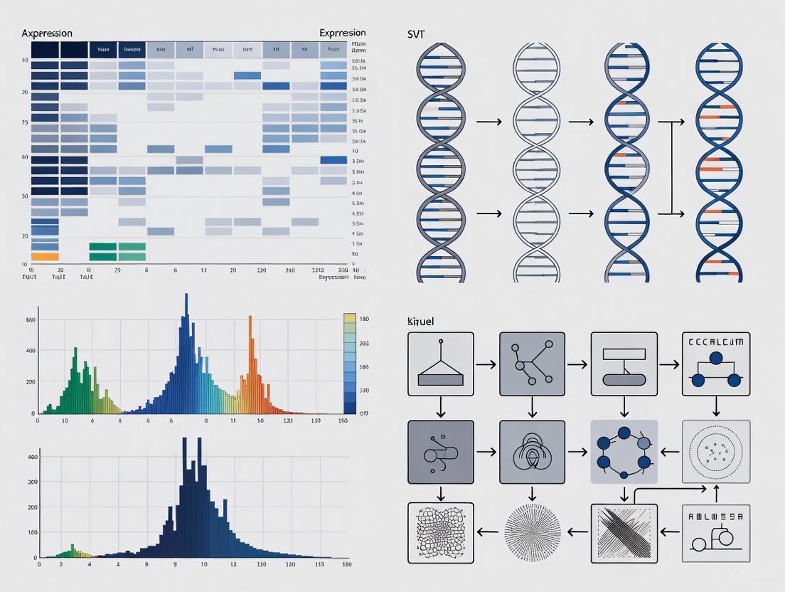
In the analysis of high-throughput genomic data, identifying informative genes is a critical first step for reducing dimensionality and enhancing the biological interpretability of downstream analyses. Two fundamental classes of such genes are Highly Variable Genes (HVGs) and Spatially Variable Genes (SVGs). HVGs are identified in single-cell RNA sequencing (scRNA-seq) data and exhibit significant expression variation across individual cells, often reflecting underlying biological heterogeneity [29] [30]. SVGs, a conceptual extension of HVGs, are identified in spatially resolved transcriptomics (SRT) data and exhibit non-random, informative spatial patterns across tissue locations [29] [31].

The detection of these variable genes is intrinsically linked to the interpretation of gene expression heatmaps. Heatmaps provide a powerful visual representation where rows typically represent genes, columns represent samples or spatial spots, and color intensity represents expression levels [2] [1]. By applying clustering algorithms to heatmaps, researchers can quickly identify groups of genes with similar expression patterns, revealing biological signatures associated with specific conditions, cell types, or spatial domains [17] [1]. This technical guide provides an in-depth examination of the methodologies for detecting HVGs and SVGs, their biological significance, and their crucial role in the interpretation of gene expression heatmaps within genomic research and drug development.

Highly Variable Genes (HVGs) in Single-Cell Analysis

Core Concepts and Biological Significance

HVG detection is a standard procedure in scRNA-seq analysis designed to filter out genes that exhibit little variation beyond technical noise, thereby focusing on genes that likely drive cellular heterogeneity [29] [30]. The fundamental assumption is that genes showing significant expression variation across single cells are more likely to reflect genuine biological differences, such as distinct cell states, types, or ongoing biological processes, rather than random technical variations from sampling effects in sequencing [29]. In practice, HVG detection screens a proportion of genes (e.g., 10–20%) with the largest variances (often adjusted for cell library sizes) to reduce the dataset's dimensionality from thousands of genes to a more manageable number of informative features [29].

The biological importance of HVGs is underscored by their strong association with cell-type-specific functions. Recent analyses have shown that HVGs are largely cell-type specific and may be modestly enriched for repressive histone marks like H3K27me3 [32]. Furthermore, increased gene expression variability itself can be a biomarker of disease states. Studies on neurodevelopmental conditions such as trisomy 21 (T21) and CHD8 haploinsufficiency have revealed a significant increase in gene expression variability in brain cell types, which is uncoupled from changes in transcript abundance and may contribute to diverse phenotypic outcomes [32].

Computational Methods for HVG Detection

Multiple computational methods have been developed for HVG detection, which can be broadly categorized into two types: those based on statistical or distributional models and those relying on clustering or graph-based approaches [30].

Table 1: Categories of HVG Detection Methods

Method Category	Description	Examples
Statistical/Distributional Models	Leverages assumptions about the relationship between mean expression and variance or dropout rates.	VST, SCTransform (Seurat) [30], M3Drop, NBDrop [30]
Clustering/Graph-Based Approaches	Identifies important genes by constructing gene-gene or cell-cell networks and applying clustering techniques.	FEAST, HRG, geneBasisR, CellBRF, DELVE [30]

A key challenge in HVG detection is the high sparsity and dropout noise characteristic of scRNA-seq data. The "dropout" phenomenon, where a gene is observed at a moderate expression level in one cell but undetected in another, arises from a complex interplay of true biological expression selectivity and technical artifacts [30].

Advanced Method: GLP for HVG Detection

The GLP (LOESS with Positive Ratio) method represents a recent advancement designed to overcome limitations posed by data sparsity. Instead of relying on variance, GLP utilizes the positive ratio (the proportion of cells in which a gene is detected) as a more robust estimator [30].

The core algorithm of GLP involves:

• Input: A gene expression count matrix (g genes × c cells).
• Calculation: For each gene j, compute its average expression level (λj) and positive ratio (fj). ( \lambdaj = \frac{1}{c}\sum{i=1}^{c} X{ij} ) ( fj = \frac{1}{c}\sum{i=1}^{c} \min(1, X{ij}) )
• LOESS Regression: Model the non-linear relationship between the positive ratio (f, independent variable) and the average expression level (λ, dependent variable) across all genes.
• Feature Selection: Genes with expression levels significantly higher than the value predicted by the LOESS regression, given their positive ratio, are selected as HVGs [30].

GLP incorporates an optimized LOESS procedure that uses the Bayesian Information Criterion (BIC) to automatically determine the optimal smoothing parameter, avoiding overfitting and enhancing the robustness of feature selection [30]. Evaluations demonstrate that GLP consistently outperforms eight other leading feature selection methods across benchmark criteria like adjusted rand index (ARI), normalized mutual information (NMI), and the silhouette coefficient [30].

Figure 1: Workflow for the GLP HVG Detection Method

Spatially Variable Genes (SVGs) in Spatial Transcriptomics

Core Concepts and Categorization of SVGs

Spatially Resolved Transcriptomics (SRT) technologies measure gene expression levels along with their spatial coordinates within a tissue, providing unprecedented insights into tissue organization and cell-cell communication [29]. SVGs are genes whose expression levels exhibit non-random, informative spatial patterns, making them crucial for understanding the spatial organization of biological processes [29] [31].

A recent comprehensive review categorizes SVGs into three distinct types based on their biological significance and the hypotheses tested by detection methods [29]:

• Overall SVGs: These genes show spatial patterns that may be driven by any underlying factor, such as multiple cell types or gradual gradients. Their detection screens informative genes for downstream analyses like identifying spatial domains or functional gene modules. The null hypothesis for their detection is that a non-SVG's expression is independent of its spatial location [29].
• Cell-Type-Specific SVGs (ct-SVGs): This subset of SVGs exhibits distinct spatial expression patterns within a specific cell type. Detecting them helps reveal spatial variation within a cell type, identifying distinct cell subpopulations or states. Methods like Celina use a spatially varying coefficient model to detect ct-SVGs by accurately capturing a gene's spatial expression in relation to cell type distribution across tissue [29] [33].
• Spatial-Domain-Marker SVGs: These genes are significantly more highly expressed in specific spatial domains (clusters of spots with similar expression profiles) and serve as marker genes to annotate and interpret these domains. Their detection is analogous to differential expression gene (DEG) detection between cell clusters in scRNA-seq analysis [29].

Table 2: Categories of Spatially Variable Genes (SVGs)

SVG Category	Primary Goal	Biological Application
Overall SVGs	Screen informative genes for downstream analysis.	Identify spatial domains and functional gene modules.
Cell-Type-Specific SVGs	Reveal spatial variation within a cell type.	Identify distinct cell subpopulations or states within a cell type.
Spatial-Domain-Marker SVGs	Find marker genes for detected spatial domains.	Annotate and interpret spatial domains, understand molecular mechanisms.

The relationship between these categories is not always straightforward. In general, if an overall SVG detection method tests for any deviation from spatial randomness, its detected SVGs should theoretically include both ct-SVGs and spatial-domain-marker SVGs [29]. However, if a method is designed to detect a specific spatial pattern (e.g., a smooth gradient), it might miss SVGs belonging to the other categories [29].

Computational Methods for SVG Detection

The field of SVG detection is rapidly evolving, with at least 34 peer-reviewed methods available [29]. These methods can be classified based on the SVG category they target, their underlying statistical paradigms (frequentist vs. Bayesian), and the types of input data they accept (count vs. normalized data) [29].

For example, DESpace is a method that can detect both overall SVGs and spatial-domain-marker SVGs [29]. As noted, Celina is specifically designed for the powerful and statistically sound detection of cell-type-specific SVGs (ct-SVGs) in both single-cell resolution and spot-resolution SRT data [33]. Its application to real datasets has successfully uncovered ct-SVGs associated with tumor progression and patient survival in lung cancer, and genes preferentially expressed near amyloid-β plaques in an Alzheimer's model [33].

The Critical Link: Interpreting Gene Expression Heatmaps

Heatmaps as a Visual Tool for Variability

A heatmap is a graphical representation of data where individual values in a matrix are represented as colors [17] [1]. In genomics, heatmaps are frequently used to visualize the expression levels of many genes across multiple samples or spatial spots [2] [1]. In a typical gene expression heatmap, each row represents a gene, each column represents a sample, and the color and intensity of each tile represent changes in gene expression (e.g., upregulation in red, downregulation in blue) [2] [1].

When a heatmap is combined with clustering, it becomes a powerful tool for visualizing the results of HVG and SVG analyses. Clustering groups genes and/or samples together based on the similarity of their gene expression patterns, making it easier to identify patterns that might otherwise be obscure in a table of numbers [2] [17] [1].

A Framework for Heatmap Interpretation

Interpreting a gene expression heatmap, particularly one displaying variable genes, involves a systematic approach [1]:

• Inspect the Axes: Identify what the rows (usually genes) and columns (usually samples or spatial spots) represent.
• Examine the Color Scale: Understand the color gradient and what expression value (e.g., log2 fold change, z-score) each color represents. This allows you to quickly distinguish upregulated from downregulated genes.
• Analyze the Clustering (Dendrograms): Observe how genes and samples are grouped. Genes clustered together have similar expression profiles across samples, suggesting co-regulation or functional relatedness. Samples clustered together have similar overall expression patterns, which may correspond to biological conditions, cell types, or spatial domains.
• Identify Patterns: Look for broad patterns. Are there blocks of color indicating groups of genes that are upregulated or downregulated in a specific set of samples? Do the sample clusters correspond to known phenotypes or spatial regions?

Figure 2: From Variable Genes to Heatmap Interpretation

For spatial transcriptomics, a heatmap of SVGs can be used to visualize and identify spatial domains. In this case, the columns of the heatmap are the spatial spots, and the dendrogram shows which spots are clustered together based on their expression of the selected SVGs. The resulting clusters of spots can be interpreted as spatial domains, which are regions of the tissue with distinct molecular profiles [29].

Essential Reagents and Computational Tools

Successfully conducting analyses for HVGs and SVGs requires a combination of wet-lab reagents and dry-lab computational tools.

Table 3: The Scientist's Toolkit for Variable Gene Analysis

Category	Item	Function and Application
Wet-Lab Reagents & Platforms	10x Genomics Chromium Single Cell 3' Kit	Library preparation for scRNA-seq to profile gene expression at single-cell resolution. [32]
	10x Visium / Xenium Platforms	Sequencing-based (Visium) and imaging-based (Xenium) SRT technologies for capturing transcriptome-wide data or targeted gene panels with spatial information. [29]
	MERFISH / seqFISH Platforms	Imaging-based SRT technologies using multiplexed error-robust fluorescence in situ hybridization for high-resolution spatial gene expression profiling. [29]
	STEMDiff SMADi Neural Induction Kit	Used for differentiating induced pluripotent stem cells (iPSCs) into neural progenitor cells (NPCs) for disease modeling in scRNA-seq studies. [32]
Computational Tools & Packages	Seurat (R)	A comprehensive toolkit for single-cell genomics, includes HVG detection methods like VST and SCTransform. [30]
	GLP (R)	A robust feature selection method using optimized LOESS regression with positive ratio for HVG detection. [30]
	Celina (R)	A statistical method for detecting cell-type-specific SVGs in spatial transcriptomics data. [33]
	DESpace (R)	A method for detecting both overall SVGs and spatial-domain-marker SVGs. [29]
	pheatmap, heatmap3 (R)	R packages for generating highly customizable, publication-quality heatmaps and dendrograms. [17] [34]

The identification of Highly Variable Genes and Spatially Variable Genes represents a foundational step in the analysis of single-cell and spatial transcriptomics data. These genes cut through the noise of high-dimensional data to reveal features of biological significance, such as cell identity, functional states, and tissue organization. As computational methods evolve—from statistical approaches like GLP for HVGs to specialized tools like Celina for ct-SVGs—our ability to pinpoint biologically relevant genes with precision continues to improve.

The power of these analyses is fully realized when combined with robust visualization techniques, particularly the clustered heatmap. A heatmap transforms the abstract numerical output of SVG and HVG detection into an intuitive visual story, allowing researchers to discern patterns of co-expression, identify novel sample clusters, and formulate hypotheses about underlying biology. For drug development professionals, this integrated process—from computational gene identification to visual pattern recognition—is indispensable for uncovering novel therapeutic targets, understanding disease morphology, and ultimately advancing personalized medicine. Mastering the interpretation of these visualizations is not merely a technical skill, but a critical component of deriving meaningful biological and clinical insights from complex genomic data.

The analysis of gene expression data represents a cornerstone of modern biological research, particularly in drug development and biomarker discovery. This technical guide outlines a comprehensive workflow for transforming raw transcriptomic data into biologically meaningful insights, with a specific focus on interpretation through gene expression heatmaps. The process encompasses data normalization, quality control, differential expression analysis, and visualization, culminating in biological interpretation that can inform therapeutic target identification [35]. Heatmaps serve as a critical visualization tool in this workflow, enabling researchers to identify patterns in gene expression across multiple samples and conditions through color gradients that represent expression levels [1] [13]. When properly executed, this analytical pipeline can reveal disease mechanisms, identify potential drug targets, and provide diagnostic or prognostic markers valuable for clinical applications [35].

Data Preprocessing and Normalization

Raw Data Processing

The initial phase of the gene expression workflow involves processing raw sequencing data into a structured format suitable for analysis. For spatial transcriptomic data generated by platforms like Nanostring GeoMx DSP, this process begins with loading Digital Cell Count (DCC) files, Protein Kinase C (PKC) files, and sample annotation files (XLSX) into the analytical environment [25]. These components are synthesized into a "GeoMxSet Object" containing the expression matrix, segment/sample annotation, probe/target annotation, and relevant metadata [25]. For RNA-sequencing data, the process typically involves aligning reads to a reference genome and generating count data for each gene across samples [36]. The initial data structure organizes genes as rows and samples as columns, creating a matrix where each cell contains the expression value for a specific gene in a particular sample [1] [13].

Normalization Methods

Normalization is a critical preprocessing step that removes technical variability while preserving biological signals. This process accounts for factors such as sequencing depth, gene length, and RNA composition that can confound accurate comparisons between samples [36]. Without proper normalization, differences in library size (total number of reads per sample) can create the false impression that genes are differentially expressed when the variation is merely technical rather than biological [36].

Table 1: Common Normalization Methods for Gene Expression Data

Method	Accounted Factors	Recommended Use Cases	Limitations
CPM (Counts Per Million)	Sequencing depth	Gene count comparisons between replicates of the same sample group	Not suitable for within-sample comparisons or DE analysis
TPM (Transcripts Per Kilobase Million)	Sequencing depth and gene length	Gene count comparisons within a sample or between samples of the same group	Not recommended for differential expression analysis
TMM (Trimmed Mean of M-values)	Sequencing depth and RNA composition	Differential expression analysis between samples	Not for within-sample comparisons; assumes most genes not differentially expressed
DESeq2's Median of Ratios	Sequencing depth and RNA composition	Differential expression analysis between samples	Not for within-sample comparisons; robust to composition bias

The TMM normalization method, implemented in edgeR, operates on the fundamental assumption that most genes in the dataset are not differentially expressed between samples [36] [35]. This method calculates scaling factors between samples by comparing each sample to a reference, typically using the trimmed mean of log expression ratios (M-values) [35]. Similarly, DESeq2's median of ratios method computes size factors for each sample by comparing each gene's count to its geometric mean across all samples, then using the median of these ratios as the normalization factor [35]. Both approaches effectively correct for differences in library size and RNA composition, ensuring that technical variations do not dominate subsequent biological interpretations [36].

Quality Control and Differential Expression Analysis

Quality Assessment

Rigorous quality control represents an essential step before proceeding to differential expression analysis. This process involves both sample-level and gene-level assessments to identify potential issues that might compromise analytical validity [36]. Sample-level QC evaluates overall similarity between samples using methods such as Principal Component Analysis (PCA) and hierarchical clustering, which help researchers determine whether samples cluster as expected based on experimental design and identify any potential outliers [36]. These methods also reveal whether the experimental condition represents the major source of variation in the dataset, as anticipated in well-designed experiments [36].

Gene-level QC focuses on filtering genes that have little chance of being detected as differentially expressed, thereby increasing statistical power for the remaining genes [36]. This filtering typically removes genes with zero counts across all samples, genes with extreme count outliers, and genes with low mean normalized counts [36]. Some differential expression tools like DESeq2 perform this filtering automatically, while others like EdgeR require explicit user specification [36]. The DgeaHeatmap package provides specific functions for data quality control, including aExprsDataQC for assessing expression data quality and show_data_distribution for visualizing data distribution to check for normality [25].

Differential Expression Analysis

Differential expression analysis identifies genes with statistically significant expression differences between experimental conditions (e.g., healthy vs. disease tissues, treated vs. untreated cells) [35]. This process employs statistical models to determine whether observed expression differences are likely to represent true biological effects rather than random variation.

Table 2: Statistical Tools for Differential Gene Expression Analysis

Tool	Underlying Distribution	Normalization Method	Key Features	Best For
edgeR	Negative binomial	TMM	Empirical Bayes estimation, exact tests tailored for over-dispersed data	Studies with biological variability, small sample sizes
DESeq2	Negative binomial	DESeq2	Shrinkage estimation of dispersion and fold changes, outlier detection	Standard RNA-seq experiments, studies with limited replicates
limma-voom	Log-normal	TMM	Linear modeling with precision weights, robust for large sample sizes	Experiments with larger sample sizes (>20 per group)
NOIseq	Non-parametric	RPKM	Noise distribution models, no assumption of data distribution	Data with complex distribution patterns

The selection of an appropriate differential expression tool depends on multiple factors, including sample size, data distribution, and experimental design [35]. Parametric methods like edgeR and DESeq2 are generally preferred for data aligning well with negative binomial distribution, which appropriately models RNA-seq count data characterized by over-dispersion [35]. These methods are particularly efficient for studies with small sample sizes, a common scenario in RNA-seq experiments due to cost constraints [35]. Non-parametric methods like NOIseq and SAMseq offer greater flexibility for datasets with complex distributions but typically require larger sample sizes for reliable results [35].

The DgeaHeatmap package incorporates multiple differential expression methods, providing functions such as DGEALimma, DGEADESeq2, and DGEAedgeR to accommodate diverse analytical preferences and data characteristics [25]. Following differential expression analysis, results extraction using functions like extractDEGenes and summarize_edgeR_DEA facilitates downstream visualization and interpretation [25].

Heatmap Generation and Visualization

Principles of Heatmap Construction

Heatmaps provide a powerful visual representation of gene expression data, transforming numerical matrices into color-coded grids that enable pattern recognition across genes and samples [1]. In a standard gene expression heatmap, rows typically represent individual genes, columns represent samples or experimental conditions, and color intensity represents expression levels [1] [13]. The transformation of numerical values to colors allows researchers to quickly identify trends that would be difficult to discern from raw numbers alone [1].

Effective heatmap construction requires several considerations, including data scaling, distance calculation, and clustering methods [17]. Data scaling, typically using Z-score transformation, ensures that genes with different expression ranges contribute equally to the visualization [25] [17]. The Z-score calculation standardizes expression values by subtracting the mean and dividing by the standard deviation for each gene, resulting in values representing the number of standard deviations from the mean [17]. This process prevents highly expressed genes from dominating the color scale and obscuring patterns in more modestly expressed genes [17].

Clustering and Distance Metrics

Clustering represents a fundamental aspect of heatmap visualization, enabling the grouping of genes with similar expression patterns and samples with similar expression profiles [1]. Hierarchical clustering is the most common approach, generating dendrograms that visually represent relationships between genes and samples [17] [13]. The clustering process involves two key decisions: selecting an appropriate distance metric and choosing a linkage method for cluster formation [17].

Distance calculation determines how similarity between expression profiles is quantified, with options including Euclidean distance (straight-line distance between points), Manhattan distance (sum of absolute differences), and correlation-based distances [17]. Each metric offers distinct advantages depending on the data characteristics and biological questions. Following distance calculation, clustering methods such as complete linkage, average linkage, or Ward's method determine how clusters are merged based on the calculated distances [17].

The DgeaHeatmap package incorporates k-means clustering as an additional approach, using elbow plots to determine the optimal number of clusters by identifying the point where the rate of variance explanation sharply decreases [25]. This method partitions genes into k clusters based on expression similarity, with the elbow point indicating the most biologically meaningful number of clusters [25].

Heatmap Generation Tools

Several computational tools are available for heatmap generation, each with distinct strengths and limitations. The pheatmap package is particularly comprehensive, offering built-in scaling functions, extensive customization options, and integrated clustering visualization [17]. Its versatility makes it suitable for creating publication-quality figures with minimal coding effort [17]. For more interactive exploration, heatmaply generates interactive heatmaps that allow users to mouse over individual tiles to view sample IDs, gene names, and expression values [17].

The DgeaHeatmap package provides specialized functions for spatial transcriptomic data, including print_heatmap, function_complexHeatmap_var, and adv_heatmap for creating heatmaps without annotation, with automatically generated annotation, or with specific user-defined annotation, respectively [25]. ComplexHeatmap offers extensive customization capabilities but requires separate data scaling before implementation [17].

Diagram 1: Gene Expression Heatmap Workflow

Biological Interpretation and Case Studies

Heatmap Interpretation Framework

Interpreting a gene expression heatmap requires systematic analysis of its components to extract biologically meaningful insights [1]. The process begins with examining the x-axis (typically samples) and y-axis (typically genes) to understand the experimental design and gene selection [1]. The color scale represents the most critical element for interpretation, with colors indicating the direction and magnitude of expression changes [1]. Typically, log2 fold change values are visualized, with positive values (often shown in red) indicating upregulation and negative values (often shown in blue) indicating downregulation [1]. The intensity of the color corresponds to the magnitude of expression change, allowing rapid identification of genes with substantial differential expression [1].

Clustering patterns provide crucial biological insights, revealing groups of genes with coordinated expression (potential co-regulation) and samples with similar expression profiles (potential biological similarities) [1]. In well-designed experiments, samples from the same experimental conditions should cluster together, validating the experimental approach [1]. Unexpected clustering patterns may reveal previously unrecognized relationships or subcategories within samples [1]. Similarly, genes clustering together may share biological functions or regulatory mechanisms, suggesting potential functional relationships [1].

Functional Enrichment Analysis

Following heatmap analysis, functional enrichment analysis contextualizes differentially expressed genes by identifying overrepresented biological processes, pathways, and molecular functions [35]. This process involves annotating genes with database identifiers and conducting statistical tests to determine whether specific biological themes are significantly represented in the gene set compared to chance expectation [35]. Pathway enrichment tools help researchers understand the molecular mechanisms underlying observed expression patterns, potentially linking gene expression changes to specific cellular processes, disease mechanisms, or drug responses [35].

The biological interpretation culminates in identifying potential biomarkers for diagnosis, prognosis, or therapeutic targeting [35]. Genes showing consistent, marked differential expression across multiple samples of a particular condition represent candidate biomarkers worthy of further investigation [35]. Similarly, genes clustered together with known disease-associated genes may represent novel players in disease pathogenesis or potential therapeutic targets [35].

Diagram 2: Biological Interpretation Process

Research Reagent Solutions

Table 3: Essential Research Reagents and Computational Tools for Gene Expression Analysis

Category	Specific Tool/Reagent	Function/Purpose	Application Context
Wet Lab Reagents	Nanostring GeoMx DSP	Spatial transcriptomics with region-specific gene expression profiling	Tissue section analysis with morphological context
RNA-seq Library Prep Kits	Various commercial kits	Convert RNA to sequencing-ready libraries	Bulk or single-cell RNA sequencing experiments
Normalization Tools	edgeR (TMM), DESeq2 (Median of Ratios)	Correct for technical variability in sequencing data	Differential expression analysis from count data
Differential Expression Tools	edgeR, DESeq2, limma	Identify statistically significant expression changes	Comparative analysis between experimental conditions
Visualization Packages	pheatmap, ComplexHeatmap, heatmaply	Generate publication-quality heatmaps	Data exploration and result presentation
Functional Analysis	Pathway enrichment tools	Biological context for differentially expressed genes	Mechanism identification and biomarker prioritization

The workflow from raw data to biological interpretation represents a critical analytical pipeline in modern molecular biology and drug development. Through systematic normalization, quality control, differential expression analysis, and thoughtful visualization via heatmaps, researchers can transform raw sequencing data into biologically actionable insights. The interpretation of gene expression heatmaps extends beyond visual pattern recognition to encompass functional enrichment analysis and biological contextualization, ultimately supporting the identification of disease mechanisms and potential therapeutic targets. As transcriptomic technologies continue to evolve, maintaining rigorous analytical approaches while effectively communicating findings through thoughtful visualization remains essential for advancing biomedical knowledge and therapeutic development.

Beyond the Basics: Solving Common Interpretation Challenges and Optimizing Visualizations

Choosing the Right Color Palette for Accurate Data Representation

In the field of genomics and drug development, heatmaps are indispensable for visualizing complex data matrices, such as gene expression patterns across multiple samples. The choice of color palette is not merely an aesthetic decision; it is a critical parameter that directly influences data interpretation, potentially leading to groundbreaking discoveries or significant misinterpretations. An inappropriately chosen color scheme can obscure biological patterns, introduce visual bias, or render findings inaccessible to colleagues with color vision deficiencies. This guide provides researchers with a scientifically-grounded framework for selecting color palettes that enhance clarity, accuracy, and accessibility in gene expression heatmaps, ensuring that visual representations faithfully communicate the underlying biological stories.

Understanding Data Nature and Color Theory

Classifying Your Data Type

The first step in selecting an appropriate color palette is to correctly identify the nature of the data you are visualizing. Biological data can be fundamentally categorized, and this classification directly dictates the most suitable color approach [37].

Quantitative data, such as gene expression values from RNA-seq (e.g., TPM values, log2 fold changes), are ordered numerical measurements. The color maps for this data type must perceptually reflect the inherent order and magnitude differences. Sequential color scales are used for data that progresses from low to high without a meaningful central point, such as raw expression counts. Diverging color scales are essential when the data has a critical central value, like zero in fold-change data, distinguishing between up-regulated and down-regulated genes [38].

Qualitative (categorical) data represents distinct classes or groups without an inherent order. Examples include cell types, tissue names, or experimental conditions. For such data, distinct hues (e.g., red, blue, green) should be used to create clear visual separation between categories [39].

Table 1: Data Types and Corresponding Color Scale Recommendations

Data Type	Description	Example in Genomics	Recommended Scale
Sequential Quantitative	Values progress uniformly from low to high	Raw TPM values, gene counts [38]	Single-hue progression (e.g., white to dark blue)
Diverging Quantitative	Values deviate from a central reference point	Standardized TPM, log2 fold change [38]	Two-hue progression from a neutral center (e.g., blue-white-red)
Qualitative/Categorical	Distinct, non-ordered categories	Cell types, treatment groups, patient cohorts	Distinct hues (e.g., red, blue, green for different conditions)

Color Spaces and Perceptual Uniformity

A color space is a model that translates colors into numbers. Common models like RGB (Red, Green, Blue) and CMYK (Cyan, Magenta, Yellow, Black) are device-dependent and not perceptually uniform, making them suboptimal for scientific visualization [37].

A color space is perceptually uniform when a change of the same numerical amount in any direction of the color space is perceived by the human eye as a change of equal visual importance. The CIE L*a*b* (CIELAB) and CIE L*u*v* color spaces, developed by the International Commission on Illumination, are respected attempts to achieve perceptual uniformity [37]. Using tools and software that leverage these color spaces helps ensure that the visual intensity of a color directly corresponds to the magnitude of the data point it represents.

Table 2: Comparison of Common Color Spaces for Data Visualization

Color Space	Model	Perceptually Uniform?	Intuitive?	Best Use Case
RGB	Additive	No	Low	Screen display, not recommended for data visualization [37]
CMYK	Subtractive	No	Low	Printing, not recommended for data visualization [37]
HSL/HSV	Transform	No	High	Quick color picking, not ideal for scientific data [37]
CIE L*a*b* / L*u*v*	Additive/Translational	Yes	Moderate	Scientific visualization, where perceptual accuracy is critical [37]

Dos and Don'ts for Heatmap Color Scales

Essential Best Practices

• Do #1: Use the Right Kind of Color Scale: Adhere to the principles outlined in Table 1. For data that is entirely positive (e.g., raw read counts), a sequential color scale is ideal. When a critical reference value exists in the middle of your data range—such as zero for fold-change or a population mean—a diverging color scale is necessary to effectively distinguish values above and below that baseline [38].
• Do #2: Prioritize Color-Blind-Friendly Palettes: Approximately 5% of the population has some form of color vision deficiency. Avoid problematic color combinations like red-green, green-brown, and blue-purple. Opt for accessible palettes that use contrast and lightness effectively, such as blue & orange or blue & red, ensuring your research is interpretable by the widest possible audience [38].

Critical Pitfalls to Avoid

• Don't #1: Use the "Rainbow" Scale: The rainbow (jet) color scale is perceptually non-linear, creating artificial boundaries where none exist in the data due to abrupt changes between hues. This can mislead viewers into perceiving sharp gradients where the underlying data changes smoothly. Furthermore, the "peak" of a rainbow scale is ambiguous (is it yellow? cyan?), making it difficult to intuitively read values [38].
• Don't #2: Overcomplicate the Palette: Excessive complexity confuses interpretation. A simple palette with a clear progression from light to dark (sequential) or from one hue through a neutral color to another hue (diverging) is most effective. Using too many unrelated hues can transform a heatmap into an uninterpretable mosaic [38].

Experimental Protocols and Workflow

A Practical Workflow for Palette Selection

The following diagram illustrates a systematic decision workflow for selecting and applying a color palette to a gene expression dataset, incorporating validation for accessibility and perceptual correctness.

Protocol: Validating a Heatmap Palette

This protocol can be incorporated into the data visualization phase of genomic analysis, such as when using tools like the exvar R package or BioVinci for generating heatmaps [38] [40].

• Data Preparation and Classification:

  • Begin with a normalized and processed gene expression matrix (e.g., normalized counts, log2-transformed values).
  • Determine the data type (sequential or diverging) based on the biological question and data structure (refer to Table 1).

• Palette Application:

  • Based on the classification, select an initial palette. For a sequential scale, a light-to-dark single hue is effective. For a diverging scale, choose two contrasting hues that meet at a neutral color at the data's midpoint.
  • Apply the palette to the heatmap using your chosen software (e.g., ggplot2 in R, matplotlib in Python, or a dedicated platform like BBrowserX [41]).

• Validation and Accessibility Assessment:

  • Check Color Context: Ensure that the colors do not create optical illusions or patterns that are not present in the data. Adjacent colors should not vibrate or create false edges [37].
  • Evaluate Perceptual Uniformity: Verify that equal steps in data value correspond to equal steps in perceived color change. This can be tested by visualizing a uniform gradient and checking for any apparent bands or jumps in color.
  • Assess Color Deficiencies: Use online simulation tools or software plugins to preview the heatmap as it would appear to individuals with common forms of color blindness, such as deuteranopia (red-green blindness). Adjust the palette if key contrasts are lost [37].

• Final Output:

  • Once the palette passes all validation checks, export the visualization in an appropriate format for publication or presentation. Verify that the color legend is clearly labeled and the figure caption describes what the colors represent.

The Scientist's Toolkit

Research Reagent Solutions for Visualization

Table 3: Essential Tools and Software for Creating Accurate Heatmaps

Tool / Reagent	Type	Function in Visualization	Example Use Case
exvar R Package [40]	Software Tool	Performs gene expression analysis and generates visualization apps (e.g., vizexp).	Integrated analysis and visualization of RNA-seq data within a single workflow.
BBrowserX [41]	Software Platform	Provides a no-code interface for single-cell data analysis and visualization, including heatmaps.	Visualizing clustered single-cell RNA-seq data with automated cell type annotation.
BioVinci [38]	Software Tool	Drag-and-drop package that allows quick customization of heatmap color scales.	Rapidly iterating and testing different color palettes on a gene expression matrix.
ColorBrewer Palettes	Color Resource	Provides a curated set of color-blind-friendly, sequential, and diverging palettes.	Selecting a scientifically validated color scheme for a publication-ready figure.
CIE L*a*b* Color Space [37]	Conceptual Framework	A perceptually uniform color model for creating and evaluating color scales.	Designing a custom sequential palette that ensures linear perceptual gradients.
Isolithocholic Acid	Isolithocholic Acid | Bile Acid Derivative | RUO	High-purity Isolithocholic Acid for research. Explore its role in bile acid metabolism & FXR signaling. For Research Use Only. Not for human use.	Bench Chemicals

The pathway to accurate data representation in gene expression heatmaps is rooted in a methodical and principled approach to color. By first understanding the nature of the data, selecting a color space that ensures perceptual uniformity, adhering to established best practices, and rigorously validating the final output for accessibility, researchers can create visualizations that are not only visually compelling but also scientifically robust and inclusive. This disciplined approach ensures that the compelling stories hidden within complex genomic datasets are communicated with clarity and precision, fostering reliable interpretation and accelerating discovery in drug development and basic research.

Addressing Overplotting and Ensuring Statistical Significance of Patterns

In the analysis of high-throughput genomic data, two fundamental challenges consistently arise: the visual cluttering known as overplotting and the statistical validation of observed patterns. Gene expression heatmaps serve as a primary tool for researchers to identify meaningful biological signatures across multiple samples or experimental conditions. However, these visualizations often become overwhelmed when displaying thousands of genes simultaneously, obscuring potential patterns and relationships. Concurrently, the risk of identifying false positive patterns increases dramatically when conducting thousands of simultaneous statistical tests in genome-wide studies. This technical guide addresses both challenges through integrated methodological frameworks, providing researchers with robust approaches for generating biologically interpretable and statistically valid insights from complex gene expression datasets.

Understanding and Addressing Overplotting

The Overplotting Problem in Gene Expression Data

Overplotting occurs when the density of data points exceeds the visual resolution of the display medium. In gene expression heatmaps, this manifests as excessive tiles in a grid where individual expression values become indistinguishable [28]. Traditional heatmaps represent genes as rows and samples as columns, with color indicating expression levels [1]. When visualizing entire transcriptomes, the standard heatmap structure may display over 20,000 genes simultaneously, resulting in a visualization that is overcrowded and suffers from diminished clarity [28]. This data overcrowding prevents researchers from detecting subtle but biologically important patterns, particularly temporal transitions and co-expression networks that operate across multiple genomic loci.

The consequences of unaddressed overplotting include:

• Loss of granularity: Fine-scale expression patterns become visually compressed
• Reduced interpretability: Biological signatures are obscured by visual noise
• Pattern masking: Coordinated expression dynamics across gene networks remain hidden
• Visual bias: Perception is drawn to the most extreme expression values only

Technical Solutions for Overplotting Mitigation

Data Reduction and Filtering Approaches

Variance-based filtering strategically reduces dataset dimensionality while preserving biologically relevant information. The methodology involves calculating the expression variance across all samples for each gene, then selecting the top N most variable genes for visualization [28]. For time-series experiments, implement correlation-based filtering by calculating Pearson correlation coefficients among genes and retaining those with r ≥ 0.5 to ensure coordinated temporal dynamics [28].

Table 1: Data Filtering Techniques for Overplotting Reduction

Technique	Methodology	Application Context	Advantages
Variance Filtering	Selects genes with highest expression variance	General differential expression	Preserves most dynamic genes
Correlation Filtering	Retains genes with Pearson r ≥ 0.5	Time-series experiments	Maintains co-expression networks
Significance Filtering	Filters by statistical thresholds (FDR < 0.05)	Hypothesis-driven research	Ensures statistical relevance
Pathway Filtering	Selects genes from predefined pathways	Pathway-centric analysis	Reduces biological bias

Advanced Visualization Alternatives

When traditional heatmaps prove inadequate despite filtering, advanced visualization methods offer enhanced pattern resolution:

Temporal GeneTerrain represents an innovative approach that transforms temporal expression data into a continuous terrain landscape [28]. The methodology involves:

• Network Construction: Building protein-protein interaction networks from selected genes
• Dimensionality Reduction: Applying the Kamada-Kawai force-directed algorithm to embed the network in two dimensions
• Expression Mapping: Projecting normalized expression values onto the fixed layout as Gaussian density fields (σ = 0.03)
• Temporal Tracking: Generating distinct terrain maps for each time-condition combination while maintaining invariant network topology

This approach enables unambiguous comparison of gene trajectories over time, effectively capturing transient waves and sustained shifts in gene activity that heatmaps obscure [28].

Clustered heatmaps incorporate hierarchical clustering to reorganize rows and columns based on expression similarity [1]. The dendrograms visually represent clustering relationships, grouping genes with similar expression profiles across samples and samples with similar expression patterns across genes [12]. This reordering brings similar elements closer together in the visualization, revealing patterns that random gene ordering would conceal.

Visualization Workflow for Addressing Overplotting

Ensuring Statistical Significance of Patterns

The Multiple Hypothesis Testing Problem in Genomics

Genome-wide expression studies conduct thousands of simultaneous statistical tests, creating a substantial risk of false positive findings. Traditional p-value thresholds (e.g., 0.05) become problematic in this context, as they control the false positive rate (FPR) per test, not across the entire experiment [42]. With a p-value cutoff of 0.05, approximately 1,000 false positives would be expected when testing 20,000 genes, potentially overwhelming true biological signals with statistical noise [42].

The fundamental distinction between error rates must be recognized:

• False Positive Rate: The probability that truly null features are called significant
• False Discovery Rate (FDR): The proportion of significant features that are truly null

This distinction becomes critical in genomics, where researchers need to identify as many significant features as possible while maintaining a relatively low proportion of false positives among those called significant [42].

Statistical Frameworks for Significance Assurance

False Discovery Rate Control

The False Discovery Rate (FDR) approach provides a more balanced framework for genome-wide studies by focusing on the proportion of significant features that are truly null rather than the rate of false positives among null features [42]. FDR methods are particularly suitable for genomic studies where many features are expected to be truly significant, as they offer a sensible balance between the number of true and false positives that is automatically calibrated and easily interpreted [42].

The q-value is defined as the FDR analogue of the p-value, representing the FDR when calling a feature significant [42]. A q-value threshold of 5% means that approximately 5% of the features called significant are expected to be false positives. This direct interpretation makes q-values particularly useful for prioritizing genes for downstream validation experiments.

Table 2: Statistical Significance Measures for Genomic Studies

Measure	Definition	Interpretation	Appropriate Thresholds
P-value	Probability of observed data if null hypothesis is true	Per-test false positive rate	Standard: 0.05, Strict: 0.001
FDR	Proportion of significant features that are truly null	Experiment-wide false positive control	Liberal: 0.1, Standard: 0.05, Strict: 0.01
Q-value	FDR when calling a feature significant	Expected false positive proportion among significant features	Standard: 0.05, Strict: 0.01

Implementation Protocols for Significance Testing

Differential Expression Analysis Protocol:

• Normalization: Apply appropriate normalization (e.g., TPM for RNA-seq, RMA for microarrays)
• Statistical Testing: Perform per-gene statistical tests (e.g., t-tests, DESeq2, limma)
• Multiple Testing Correction: Apply Benjamini-Hochberg procedure to control FDR
• Q-value Calculation: Estimate q-values using storey's method or similar approaches
• Threshold Application: Apply q-value threshold (typically ≤ 0.05) to determine significance

Clustering Significance Validation:

• Cluster Generation: Perform hierarchical clustering using complete linkage and Euclidean distance
• Stability Assessment: Apply bootstrap resampling to assess cluster stability
• P-value Calculation: Compute approximately unbiased p-values for cluster nodes
• Significant Cluster Selection: Retain clusters with p-value ≥ 0.95 for high confidence

Statistical Validation Workflow for Gene Expression Patterns

Integrated Analytical Framework

Comprehensive Workflow for Pattern Discovery

The synergistic application of overplotting solutions and statistical validation creates a robust framework for reliable pattern discovery in gene expression data. The recommended integrated workflow:

• Preprocessing and Quality Control

  • Perform normalization and batch effect correction
  • Conduct quality assessment using PCA and sample correlation analysis
  • Remove outliers and low-quality samples

• Dimensionality Reduction

  • Apply variance-based filtering (select top 1,000-5,000 most variable genes)
  • Implement correlation-based filtering for time-series data (r ≥ 0.5)
  • Optionally apply pathway-based filtering for hypothesis-driven research

• Statistical Significance Analysis

  • Conduct differential expression testing with appropriate models
  • Apply FDR correction using Benjamini-Hochberg procedure
  • Calculate q-values for each gene
  • Filter results using dual thresholds (e.g., |log2FC| > 1 and q-value < 0.05)

• Visualization and Pattern Validation

  • Generate clustered heatmaps with hierarchical clustering
  • Assess cluster stability via bootstrap resampling
  • For temporal data, apply Temporal GeneTerrain for dynamic visualization
  • Validate patterns through enrichment analysis and literature correlation

Table 3: Key Research Reagent Solutions for Gene Expression Heatmap Analysis

Resource Category	Specific Tools/Platforms	Function and Application
Bioinformatics Databases	NCBI GEO, ArrayExpress	Public repository for gene expression data storage and retrieval
Online Analysis Tools	ClustVis, HeatmapGenerator	Web-based tools for heatmap generation and multivariate data visualization
Statistical Frameworks	R/Bioconductor, Python SciPy	Computational environments for FDR control and q-value estimation
Visualization Software	Temporal GeneTerrain, ComplexHeatmap	Advanced platforms for dynamic and clustered heatmap visualization
Clustering Algorithms	Hierarchical Clustering, k-means	Methods for identifying groups of genes with similar expression patterns

The interpretation of gene expression heatmaps in research requires meticulous attention to both visual clarity and statistical rigor. Through the integrated application of data reduction techniques, advanced visualization methods, and robust statistical frameworks, researchers can transform overwhelming datasets into biologically meaningful insights. The methodologies presented in this guide provide a comprehensive approach to addressing the dual challenges of overplotting and statistical significance, enabling more reliable pattern discovery and interpretation in genomic research. As visualization technologies continue to evolve, maintaining this balance between visual representation and statistical validation will remain fundamental to extracting valid biological knowledge from increasingly complex and high-dimensional gene expression datasets.

Cluster analysis, particularly when visualized through heatmaps and dendrograms, serves as a fundamental tool in genomic research for identifying patterns in high-dimensional data. However, the interpretation of these dendrograms is fraught with potential pitfalls that can lead to erroneous biological conclusions. This technical guide examines the critical factors influencing dendrogram construction and interpretation within gene expression studies, providing researchers and drug development professionals with a framework for robust analysis. We detail methodological considerations, present comparative data on clustering approaches, and establish best practices to prevent misinterpretation, ensuring that conclusions drawn from heatmap visualizations accurately reflect underlying biological phenomena rather than analytical artifacts.

In the analysis of complex genomic data, clustered heatmaps have become an indispensable visualization tool, effectively combining a color-coded matrix with hierarchical clustering results displayed as dendrograms. These visualizations allow researchers to simultaneously observe expression patterns across thousands of genes and multiple samples, identifying potential subtypes, biomarkers, and functional relationships [18]. The dendrogram, a tree-like structure adjacent to the heatmap, represents the hierarchical relationships and similarity between genes (row dendrogram) or samples (column dendrogram) based on a chosen distance metric and clustering algorithm [17] [18].

The power of this combined visualization is evident across numerous biological applications, from identifying cancer subtypes based on gene expression profiles [18] to revealing metabolic patterns in neurological diseases [18]. In drug development, clustered heatmaps can stratify patient populations according to molecular signatures, potentially predicting treatment response [18]. However, this analytical power comes with significant responsibility—misinterpretation of dendrograms can lead to false discoveries, incorrect patient stratification, and ultimately, misguided research directions or clinical decisions.

Fundamental Concepts and Potential Pitfalls

The Anatomy of a Clustered Heatmap

A properly constructed clustered heatmap consists of three integrated components:

• Heat Map Matrix: The main grid where each cell's color represents normalized gene expression values, typically with rows representing genes and columns representing samples or experimental conditions [18].
• Dendrogram: Tree-like structures showing hierarchical clustering of rows and columns, where the branch lengths represent the degree of similarity between clusters [17] [18].
• Metadata Annotations: Additional bars adjacent to the heatmap that color-code sample characteristics (e.g., treatment group, disease subtype) or gene properties, enabling correlation of cluster patterns with external variables [43].

Several critical factors can lead to misinterpretation of dendrograms in gene expression studies:

• Distance Metric Selection: The choice of distance metric (Euclidean, Manhattan, Pearson correlation) fundamentally influences cluster formation [44]. Genes or samples may cluster together under one metric but separate under another, potentially leading to different biological interpretations.
• Clustering Method Bias: Different linkage methods (complete, single, average) produce distinct dendrogram structures [44]. Complete linkage tends to create compact clusters, while single linkage can produce "chaining" effects that may not reflect true biological relationships [44].
• Scale Sensitivity: Data scaling decisions dramatically impact clustering results [17]. Without proper normalization, highly expressed genes can dominate the cluster structure, obscuring patterns in more modestly expressed but biologically relevant genes [17].
• Visual Perception Limitations: The human eye naturally seeks patterns, potentially identifying "clusters" that represent random variations rather than true biological signals [18].

Table 1: Common Distance Metrics and Their Appropriate Applications in Gene Expression Studies

Distance Metric	Mathematical Basis	Appropriate Use Cases	Limitations
Euclidean	Straight-line distance between points in n-dimensional space	Identifying genes with similar absolute expression levels across samples	Sensitive to outliers; assumes data is isotropically distributed
Manhattan	Sum of absolute differences along coordinate axes	Robust analysis when outliers are present; better for high-dimensional data	Can produce axis-aligned clusters that may not reflect biological relationships
Pearson Correlation	Measures linear relationship between expression profiles	Finding genes with similar expression patterns regardless of absolute magnitude	May miss non-linear relationships; sensitive to background noise

Methodological Framework for Robust Analysis

Data Preprocessing Protocol

Proper data preparation is essential before initiating cluster analysis:

• Data Cleaning: Address missing values using appropriate methods such as k-nearest neighbor imputation or complete case analysis, documenting the approach and potential biases introduced [45].
• Normalization and Scaling: Apply Z-score standardization to rows (genes) to ensure comparability across features with different expression levels using the formula: z = (individual value - mean) / standard deviation [17]. This prevents highly expressed genes from dominating the cluster structure.
• Feature Selection: Filter genes to include biologically relevant features (e.g., differentially expressed genes, highly variable genes) to reduce noise and computational complexity [45] [19].

Hierarchical Clustering Workflow

The following workflow outlines the key decision points in hierarchical clustering analysis:

Diagram 1: Hierarchical clustering analysis workflow with key decision points

Experimental Validation Protocol

To ensure clustering results reflect biological reality rather than analytical artifacts, implement this validation protocol:

• Cluster Stability Assessment:

  • Apply resampling techniques (bootstrapping or jackknifing) to evaluate the consistency of cluster assignments.
  • Calculate the Jaccard similarity index between clusters generated from full data and resampled data.
  • Accept clusters with similarity indices >0.75 as robust.

• Biological Validation:

  • Test for enrichment of known biological pathways within clusters using gene ontology analysis [40].
  • Validate cluster-specific markers using independent experimental methods (e.g., RT-qPCR for gene expression clusters).
  • Correlate cluster assignments with clinical outcomes in patient studies when available.

• Parameter Sensitivity Analysis:

  • Systematically vary distance metrics and linkage methods.
  • Document how cluster assignments change with different analytical choices.
  • Report the range of stable clusters across parameters.

Table 2: Comparison of Hierarchical Clustering Linkage Methods

Linkage Method	Cluster Formation Approach	Advantages	Disadvantages	Recommended For
Complete	Measures maximum distance between clusters	Creates compact, evenly-sized clusters; less sensitive to noise	Can overly separate outliers; tends to break large clusters	General gene expression analysis where distinct subgroups are expected
Average	Uses mean distance between all inter-cluster pairs	Balanced approach; relatively robust	Computationally intensive; can produce uneven cluster sizes	Large datasets with expected gradual transitions between states
Single	Uses minimum distance between clusters	Can identify unusual shapes and connected structures	Highly sensitive to noise; creates "chaining" artifacts	Identifying rare cell populations or continuous differentiation processes

Technical Implementation Guide

Software Tools and Implementation

Multiple computational tools are available for generating clustered heatmaps, each with distinct capabilities:

• pheatmap (R): Provides comprehensive features with built-in scaling, automatic legend generation, and extensive customization options for publication-quality figures [17].
• ComplexHeatmap (R): Supports complex annotations and multiple heatmap integrations, ideal for advanced genomic applications [18].
• seaborn.clustermap (Python): Generates clustered heatmaps with automatic dendrogram generation within the Python ecosystem [18].
• NG-CHM (Next-Generation Clustered Heat Maps): Offers interactive features including zooming, panning, and dynamic data exploration beyond static heatmaps [18].

Research Reagent Solutions

Table 3: Essential Analytical Tools for Cluster Analysis in Genomic Studies

Tool/Category	Specific Examples	Function/Purpose	Considerations
Clustering Algorithms	Hierarchical clustering (hclust), K-means, Model-based clustering	Groups genes or samples with similar expression patterns	Choice depends on data structure and research question; hierarchical clustering provides dendrograms for visualization
Distance Metrics	Euclidean, Manhattan, Pearson correlation, Spearman correlation	Quantifies similarity between gene expression profiles	Different metrics emphasize different aspects of similarity; test multiple options
Data Preprocessing Tools	DESeq2, edgeR, limma (R packages)	Normalizes raw count data to remove technical artifacts	Essential for removing biases before clustering; method depends on sequencing technology
Visualization Packages	pheatmap, ComplexHeatmap, heatmaply (R), seaborn (Python)	Generates publication-quality heatmaps with dendrograms	heatmaply provides interactive features for data exploration [17]
Statistical Validation	pvclust (R), fpc (R)	Assesses cluster stability and significance	Provides confidence intervals for dendrogram nodes; crucial for interpretation

Comprehensive R Code Implementation

The following R code demonstrates a robust approach to clustered heatmap generation with multiple validation steps:

Interpretation Guidelines and Best Practices

Dendrogram Interpretation Framework

Proper interpretation of dendrograms requires understanding both the visual representation and statistical underpinnings:

• Branch Length Significance: Longer horizontal branches indicate greater dissimilarity between clusters. However, absolute lengths are influenced by the distance metric used and should be interpreted relative to other branches in the same dendrogram [18].
• Cluster Stability Assessment: Utilize statistical measures like bootstrap p-values or approximately unbiased (AU) values to identify robust clusters. Clusters with AU > 0.95 have strong statistical support [18].
• Cut Point Selection: Determine where to cut the dendrogram to define discrete clusters based on biological knowledge, statistical support, and research objectives rather than arbitrary height selection [19].

Contextual Integration of Results

Clustered heatmaps should never be interpreted in isolation. Implement these integrative practices:

• Metadata Correlation: Systematically correlate cluster assignments with sample metadata (e.g., clinical variables, treatment groups) to identify biologically meaningful patterns [43].
• Functional Enrichment Analysis: For gene clusters, perform gene ontology or pathway enrichment analysis to determine if co-clustered genes share biological functions [40].
• Multi-Method Verification: Confirm key findings using alternative clustering approaches (e.g., k-means, model-based clustering) to ensure results are method-independent [45].

The relationship between analytical decisions and interpretation challenges can be visualized as follows:

Diagram 2: Relationship between analytical decisions and interpretation outcomes

The interpretation of dendrograms in clustered heatmaps represents a critical juncture in genomic data analysis where analytical decisions directly influence biological conclusions. By implementing a rigorous methodology that includes careful selection of distance metrics, validation of clustering stability, and integration of biological context, researchers can avoid common misinterpretation pitfalls. The frameworks and protocols presented in this guide provide a pathway to more robust, reproducible, and biologically meaningful cluster analysis in gene expression studies. As clustering methodologies continue to evolve with advances in single-cell technologies and multi-omics integration [46], maintaining methodological rigor and interpretive caution remains paramount for extracting valid insights from complex genomic datasets.

Best Practices for Annotating Heatmaps to Enhance Readability and Insight

In gene expression analysis, a heatmap is a powerful visualization tool that represents a matrix of data, typically from RNA-seq or microarray experiments, as a grid of colored tiles. Each row usually represents a gene, and each column represents a sample or experimental condition [1] [13]. The color and intensity of each tile represent changes in gene expression levels, allowing researchers to quickly identify patterns across many genes and samples simultaneously [1].

The primary value of a clustered heatmap lies in its combination with clustering methods, which perform a meaningful reordering of the rows and columns. This process groups together genes with similar expression profiles and samples with similar expression patterns, making it dramatically easier to visualize biological relationships [1] [13]. For example, in a cancer study, clustering will often group cancer samples separately from healthy controls and cluster genes that are coordinately upregulated or downregulated in the disease state [1].

Core Principles of Effective Heatmap Annotation

Effective annotation transforms a standard heatmap from a simple graphic into a scientifically rigorous and interpretable figure. Proper annotation provides the necessary context for readers to understand the experimental design and the biological story the data tells.

The Role of Dendrograms and Labels

Clustered heatmaps are often paired with dendrograms, which are tree-like diagrams that illustrate the results of the hierarchical clustering algorithm. The dendrogram's branch lengths represent the degree of similarity between genes or samples, with shorter branches indicating higher similarity [1] [13]. Annotating these dendrograms with clear labels is crucial. For samples, this includes condition, replicate, and batch information. For genes, this includes gene symbols and descriptive names.

Utilizing Color Scales

The color scale is the legend that maps color to numerical value. In gene expression, this is often the log2 fold change or a Z-score of normalized expression [1]. The scale must be:

• Intuitive: Typically, a diverging color scheme is used where one color (e.g., red) represents upregulated genes, another (e.g., blue) represents downregulated genes, and a neutral color (e.g., white) represents no change [1].
• Accessible: The color palette should be chosen with color-blind users in mind, avoiding problematic combinations like red-green [1].
• Clearly Labeled: The scale must have a descriptive title and clearly marked numerical values.

A Methodological Protocol for Heatmap Creation and Annotation

Below is a detailed, step-by-step protocol for creating and annotating a gene expression heatmap, from data preparation to final interpretation.

Protocol: Generating an Annotated Clustered Heatmap

I. Data Preparation and Preprocessing

• Data Source: Begin with a matrix of normalized gene expression values (e.g., TPM, FPKM, or normalized counts from RNA-seq) or differential expression statistics (e.g., log2 fold change). The matrix should have genes as rows and samples as columns [1].
• Data Filtering: Filter the gene list to focus on the most informative genes. This often involves selecting genes that are differentially expressed (based on p-value and fold change thresholds) or genes from a pathway of interest. This reduces noise and enhances clarity.
• Data Transformation: For visualization, it is common to transform the data. This can involve:
  • Z-score normalization: Scaling expression for each gene across samples to have a mean of zero and a standard deviation of one. This highlights relative expression patterns for each gene [1].
  • Log2 Transformation: Applying a log2 transformation to fold-change values to center the data and make the distribution more symmetrical.

II. Clustering and Visualization

• Select Clustering Method: Choose a clustering algorithm. Hierarchical clustering is the most common method for heatmaps, which generates the accompanying dendrograms [1] [13].
• Choose Distance Metric and Linkage Method:
  • Common distance metrics include Euclidean distance (for absolute differences) or correlation-based distance (for pattern similarity).
  • Common linkage methods include Ward's method, complete linkage, or average linkage. The choice can affect cluster structure and should be documented.
• Generate Initial Heatmap: Using a bioinformatics tool, generate the initial heatmap with clustering. The output should include the main heatmap, row and column dendrograms, and a color scale.

III. Annotation and Enhancement

• Add Sample Annotations: Create a colored annotation bar above or below the column dendrogram. Each color band represents a different experimental variable (e.g., disease state, tissue type, treatment). This directly links sample metadata to the clustering results [13].
• Add Gene Annotations: Similarly, create an annotation bar alongside the row dendrogram to indicate gene-level metadata, such as gene function, pathway membership, or chromosome location.
• Refine Labels and Scale:
  • Ensure all labels (sample names, gene names) are legible. For large heatmaps with hundreds of genes, it may be impractical to show every gene name; instead, the overall pattern is the focus [1].
  • Verify the color scale is clearly titled and labeled with the units (e.g., "Z-score of normalized expression" or "log2(Fold Change)").

IV. Validation and Interpretation

• Interpret Clusters: Identify the main gene and sample clusters. Describe the expression pattern of key gene clusters (e.g., "Genes in cluster A are highly expressed in all cancer samples").
• Relate to Biology: Correlate the clustered patterns with the sample annotations and known biology. Are the sample clusters driven by expected experimental conditions? Do the gene clusters correspond to known functional pathways?
• Validate Findings: Use the heatmap as a guide for further biological validation. Genes of interest identified in specific clusters can be taken forward for functional experiments.

Experimental Workflow

The following diagram illustrates the key stages of this protocol.

The following table details key reagents, software, and databases essential for conducting a gene expression heatmap analysis.

Table 1: Research Reagent Solutions for Heatmap Analysis

Item Name	Function / Application
Normalized Gene Expression Matrix	The primary input data for the heatmap, containing normalized expression values (e.g., TPM, FPKM) for genes (rows) across samples (columns) [1].
Sample Metadata	Structured data describing the experimental attributes of each sample (e.g., phenotype, treatment, batch). Crucial for creating meaningful sample annotations [13].
ClustVis	A web tool for visualizing clustering of multivariate data using Principal Component Analysis (PCA) and heatmaps [13].
HeatmapGenerator	A software suite for high-performance RNAseq and microarray visualization to examine differential gene expression levels [13].
Gene Ontology (GO) Database	A major resource for functional annotation of genes. Used to ascribe biological meaning to clusters of co-expressed genes identified in the heatmap [13].
KEGG Pathway Database	A collection of pathway maps representing molecular interaction and reaction networks. Used for pathway enrichment analysis of gene clusters [13].

Advanced Annotation: Interpreting Patterns and Avoiding Pitfalls

A Framework for Visual Interpretation

A systematic approach to looking at a heatmap ensures no critical insight is missed.

Table 2: Heatmap Interpretation Checklist

Step	Focus Area	Key Questions
1. Check Axes & Labels	Sample (X) and Gene (Y) Axes	What are the experimental conditions? Are the sample groups clustering as expected? [1]
2. Read the Color Scale	Legend/Key	What do the colors represent (e.g., Z-score, log2FC)? What is the magnitude of change? [1]
3. Identify Sample Clusters	Column Dendrogram	Do samples from the same condition cluster together? Are there any unexpected sample groupings? [1] [13]
4. Identify Gene Clusters	Row Dendrogram	Which groups of genes have similar expression patterns across samples? How many distinct gene clusters are there? [1] [13]
5. Correlate Patterns	Main Heatmap Body	How do the gene expression patterns align with the sample clusters? (e.g., "Is the red gene cluster highly expressed in the blue sample group?") [1]

Logical Flow for Data Interpretation

The process of drawing conclusions from a heatmap follows a logical pathway from observation to biological hypothesis, as shown below.

A well-annotated heatmap is more than just a publication requirement; it is a critical tool for discovery. By meticulously applying the practices of data preparation, clustering, and annotation detailed in this guide, researchers can transform complex gene expression matrices into clear, insightful visual narratives. This clarity is fundamental for generating robust biological hypotheses, ultimately accelerating progress in biomedical research and drug development.

Ensuring Robustness: Validation Techniques and the Future with AI Prediction Models

In the field of spatial biology, the accurate identification of spatially variable genes (SVGs) is a fundamental task that enables researchers to understand tissue morphology, cellular communication, and disease mechanisms. As spatially resolved transcriptomics (SRT) technologies have advanced, numerous computational methods have been developed to detect genes with non-random spatial expression patterns. The performance of these methods varies significantly depending on the data characteristics and analytical goals, making comprehensive benchmarking essential for methodological selection and advancement. Benchmarking studies systematically evaluate these computational methods using realistic datasets and multiple performance metrics to provide guidance for researchers and developers alike. Proper benchmarking allows scientists to select the most appropriate methods for their specific research contexts, ultimately enhancing the biological insights gained from spatial transcriptomics data [47] [48].

The interpretation of gene expression heatmaps, a common visualization tool in transcriptomics, is deeply connected to the quality of the underlying spatial gene identification. Accurate detection of spatially variable genes ensures that heatmaps reflect true biological patterns rather than technical artifacts or random noise. This technical guide examines the core metrics and methodologies used to evaluate predictive performance in spatial gene expression analysis, providing researchers with the framework needed to critically assess computational tools and interpret their results within the broader context of gene expression research.

Core Metrics for Evaluating Predictive Performance

Benchmarking studies employ multiple metrics to evaluate different aspects of predictive performance, as no single metric can fully capture the effectiveness of spatial gene detection methods. The most commonly used metrics assess the accuracy of gene expression prediction, the similarity of spatial patterns, and the ability to distinguish true signals from noise.

Table 1: Key Metrics for Evaluating Spatial Gene Expression Predictions

Metric	Full Name	Interpretation	Optimal Value
PCC (Pearson Correlation Coefficient)	Pearson Correlation Coefficient	Measures linear correlation between predicted and true expression values	+1 (perfect positive correlation)
MI (Mutual Information)	Mutual Information	Quantifies statistical dependency between predicted and true expression, capturing non-linear relationships	Higher values indicate stronger dependency
SSIM (Structural Similarity Index)	Structural Similarity Index	Assesses perceptual similarity and pattern preservation between spatial expressions	+1 (identical structural information)
AUC (Area Under the Curve)	Area Under the ROC Curve	Evaluates classification performance in distinguishing zero vs. non-zero expression	+1 (perfect classification)

In practice, these metrics are applied to evaluate how well predicted spatial gene expression patterns match ground truth data. For example, a recent benchmarking study evaluating methods that predict spatial gene expression from histology images reported PCC values ranging from 0.28 for the best-performing method (EGNv2) to lower values for other methods across the same datasets. The same study found that methods generally performed better on spatially variable genes (SVGs) and highly variable genes (HVGs) compared to all genes, with most methods showing statistically significant improvements (p < 0.05) for these biologically relevant gene subsets [27].

The SSIM metric is particularly valuable for spatial transcriptomics as it captures the preservation of spatial patterns and structures in the tissue. In benchmarking analyses, methods with higher SSIM values better maintain the spatial relationships and morphological features that are crucial for biological interpretation. Similarly, AUC values indicate how well a method can distinguish between expressed and non-expressed genes across spatial locations, which is fundamental for downstream analyses like spatial domain detection and differential expression testing [27].

Benchmarking Results for SVG Detection Methods

Comprehensive Performance Evaluation

Large-scale benchmarking studies have evaluated numerous SVG detection methods across multiple datasets and performance dimensions. One comprehensive analysis assessed 14 computational methods using 96 spatial datasets and 6 evaluation metrics, focusing on gene ranking capability, statistical calibration, computational scalability, and impact on downstream applications. The results revealed that SPARK-X generally outperformed other methods, while Moran's I also achieved competitive performance, establishing a strong baseline for future method development [47].

Another extensive benchmarking framework evaluated 15 SVG identification methods using 30 synthesized and 74 real-world datasets from various spatial technologies. This study evaluated methods across five critical aspects: SVG detection accuracy, statistical validity, clustering accuracy in downstream analysis, stability, and computational scalability. The findings highlighted that method performance varies significantly across different data types and evaluation criteria, emphasizing the importance of context-specific method selection [48].

Table 2: Performance Comparison of Selected SVG Detection Methods

Method	Statistical Approach	Key Strengths	Notable Performance Findings
SPARK-X	Correlation-based	Computational efficiency, strong overall performance	Top performer in comprehensive benchmarking [47]
Moran's I	Spatial autocorrelation	Simple, interpretable, strong baseline	Competitive performance across multiple metrics [47]
SPARK	Generalized linear spatial model	Robust statistical approach for count data	Good detection power for complex spatial patterns [47]
SpatialDE	Gaussian process regression	Pioneer method, foundational approach	Lower computational efficiency than newer methods [47]
SOMDE	Self-organizing map + Gaussian process	High scalability for large datasets	Best performance across memory usage and running time [47]

Impact on Downstream Applications

The identification of spatially variable genes has significant implications for downstream analyses in spatial transcriptomics. Benchmarking studies have demonstrated that using SVGs generally improves spatial domain detection compared to using highly variable genes (HVGs) alone. This enhancement is crucial for applications such as tissue region segmentation, characterization of tumor microenvironments, and understanding developmental biology [47].

Furthermore, benchmarking revealed that most methods except for SPARK and SPARK-X produced inflated p-values, indicating poor statistical calibration. This finding highlights the importance of proper statistical calibration in method development and the need for researchers to consider false discovery control when interpreting results [47].

Experimental Protocols for Benchmarking Studies

Dataset Selection and Preparation

Robust benchmarking requires diverse and biologically realistic datasets. The following protocols are commonly employed in comprehensive benchmarking studies:

• Real Data Collection: Curate multiple real-world spatial transcriptomics datasets from different technologies (e.g., 10x Visium, Slide-seq, MERFISH, seqFISH) covering various tissue types and spatial resolutions. One benchmarking framework assembled 74 real datasets for this purpose [48].
• Realistic Data Simulation: Employ advanced simulation frameworks like scDesign3 that use real data as references to generate biologically realistic spatial transcriptomics data. This approach models gene expression as a function of spatial locations using Gaussian Process models, then randomly shuffles parameters to create non-spatial controls [47].
• Silver Standard Construction: When true gold standards are unavailable, construct multiple "silver standard" gene sets using complementary approaches:
  • Spatial auto-correlation using Moran's I
  • Differential expression between expert-annotated spatial domains using Wilcoxon test
  • Negative binomial regression between spatial domains
  • Correlation with H&E-stained histology images [48]

Evaluation Framework Implementation

Comprehensive benchmarking requires a multi-faceted evaluation strategy:

• Performance Metrics Calculation: Compute PCC, MI, SSIM, and AUC for each method across all datasets, focusing on both overall performance and performance on biologically relevant gene subsets (HVGs and SVGs) [27].
• Statistical Validation: Assess statistical calibration through p-value uniformity tests and false discovery rate control under null scenarios [47].
• Downstream Analysis Impact: Evaluate how identified SVGs affect performance in applications like spatial domain detection using clustering methods such as Louvain algorithm and spatial-aware methods like BayesSpace [48].
• Scalability Assessment: Measure computational requirements including running time and memory usage across datasets of varying sizes [47].

Visualization of Benchmarking Workflows

SVG Method Classification and Workflow

Comprehensive Benchmarking Evaluation Framework

The Scientist's Toolkit: Essential Research Reagents and Computational Solutions

Table 3: Key Computational Tools for SVG Detection and Evaluation

Tool/Resource	Type	Primary Function	Application Context
SPARK-X	SVG Detection Method	Identifies SVGs by comparing expression and spatial covariance matrices	General-purpose SVG detection with high efficiency [47]
Moran's I	Spatial Statistic	Measures spatial autocorrelation of gene expression	Establishing performance baselines, simple analyses [47]
scDesign3	Simulation Framework	Generates biologically realistic spatial transcriptomics data	Benchmarking and method validation [47]
SpatialDE	SVG Detection Method	Gaussian process regression for testing spatial patterns	Foundational approach, comparative analyses [47] [48]
SOMDE	SVG Detection Method	Self-organizing map combined with Gaussian process	Large-scale data analysis with computational efficiency [47]
H&E-Stained Images	Histology Reference	Provides morphological context for spatial validation	Silver standard construction, biological validation [48]

Gene expression heatmaps are a cornerstone of genomic visualization, powerfully revealing co-expression patterns and sample clusters through hierarchical clustering [18]. However, the identified patterns themselves are purely statistical constructs—they do not automatically imply biological relevance or mechanistic relationships. The critical step of biological validation transforms these visual patterns into meaningful insights about disease mechanisms, therapeutic targets, and fundamental biology.

This technical guide provides researchers with a systematic framework for connecting heatmap-derived patterns to established biological pathways and functions. By implementing rigorous validation protocols, scientists can distinguish biologically significant findings from statistical artifacts and build robust conclusions for publication and drug development projects.

Core Interpretation Workflow

The journey from raw heatmap to biological insight follows a structured pathway encompassing visualization, statistical analysis, and functional validation, as outlined below.

Initial Heatmap Interpretation

A clustered heatmap integrates two primary techniques: heat mapping and hierarchical clustering [18]. The visualization consists of:

• Heat Map Matrix: A grid where each cell's color represents normalized gene expression values, typically with upregulated genes in red and downregulated genes in blue [2].
• Dendrograms: Tree-like structures displaying hierarchical clustering results of rows (genes) and columns (samples) based on chosen similarity measures [18].
• Row and Column Labels: Identifiers for genes and samples, respectively [18].

Proper interpretation requires understanding that clusters represent statistical similarities rather than confirmed biological relationships. These patterns must be validated with additional statistical methods and experimental approaches [18].

Pathway Analysis Methodologies

Gene Set Enrichment Analysis

Gene set enrichment analysis (GSEA) functionally annotates differentially expressed genes to determine if they associate with specific biological processes or molecular functions [2]. This method compares the frequency of individual annotations in your gene list against a reference list (typically all genes on the array or in the genome).

Table 1: Primary Enrichment Analysis Types

Analysis Type	Data Source	Key Output	Common Tools
Gene Ontology (GO) Enrichment	Gene Ontology database	Biological processes, molecular functions, cellular components	clusterProfiler, topGO, DAVID
Pathway Enrichment	KEGG, Reactome, WikiPathways	Signaling/metabolic pathways, disease pathways	IPA, ReactomePA, Pathview
Upstream Regulator Analysis	Literature-mined regulatory networks	Potential transcription factors, cytokines controlling expression	IPA, Enrichr
Disease Association Enrichment	Disease databases, OMIM	Associations with pathological conditions	DisGeNET, DOSE

Practical Implementation Protocol

Protocol 1: Functional Enrichment Analysis

• Input Preparation: Start with a statistically significant differentially expressed gene (DEG) list, including identifiers (e.g., Ensembl IDs, official gene symbols), expression fold changes, and p-values. For RNA-seq data, ensure proper normalization has been applied (e.g., TMM in edgeR or geometric mean in DESeq2) [35].

• Tool Selection: Choose an enrichment tool based on your experimental design and biological questions. For comprehensive analysis, use multiple complementary tools.

• Parameter Configuration:

  • Set significance thresholds (adjusted p-value < 0.05, FDR < 0.25 for GSEA)
  • Apply appropriate multiple testing corrections (Bonferroni, Benjamini-Hochberg)
  • Define minimum/maximum gene set sizes (typically 5-500 genes per set)

• Execution and Iteration: Run analyses across multiple databases to identify consensus pathways. Repeat with different stringency settings to ensure robust findings.

• Results Interpretation: Prioritize enriched terms based on statistical significance, degree of enrichment (fold enrichment), and biological plausibility in your experimental context.

Advanced Validation Techniques

Multi-Omics Integration and Comparison Analysis

Advanced validation often requires integrating multiple datasets or experimental conditions. Comparison Analysis enables visualization across multiple analyses with varying conditions (e.g., dose response, time course) to identify consistent patterns or trends [49].

Table 2: Experimental Reagents for Validation

Reagent/Method	Application	Experimental Function	Key Considerations
siRNA/shRNA Knockdown	Functional validation	Tests necessity of candidate genes in pathway activity	Off-target effects; compensation
CRISPR-Cas9 Knockout	Functional validation	Determines necessity with complete gene disruption	Complete knockout may be lethal
qRT-PCR Reagents	Technical validation	Confirms expression changes of key targets	Use multiple reference genes
Western Blot Reagents	Protein-level validation	Confirms regulation at protein level	Antibody specificity critical
Immunofluorescence Assays	Spatial validation	Localizes protein expression in tissue context	Quantification challenges
Chromatin Immunoprecipitation (ChIP)	Mechanistic validation	Direct TF binding to promoter regions	Antibody quality dependent

The workflow for multi-analysis comparison can be visualized as:

Network Analysis Implementation

Protocol 2: Network-Based Validation

Network analysis complements pathway analysis by showing how key components from different pathways interact, identifying regulatory events that influence multiple biological processes simultaneously [2].

• Data Input Preparation: Start with significantly enriched pathways and their constituent genes, plus upstream regulator analysis results if available.

• Network Construction:

  • Import gene lists into network analysis tools (Cytoscape, IPA)
  • Connect genes based on:
    • Protein-protein interactions (StringDB, BioGRID)
    • Regulatory relationships (transcription factor-target)
    • Signaling pathways (KEGG, Reactome)
  • Overlay expression data (fold changes) as visual attributes

• Topology Analysis:

  • Identify network hubs (highly connected nodes)
  • Calculate betweenness centrality (bottleneck genes)
  • Detect functional modules using cluster algorithms

• Key Node Prioritization: Focus validation efforts on genes that:

  • Serve as hubs in the network
  • Connect multiple enriched pathways
  • Have literature support for relevant biological roles
  • Are druggable targets (for therapeutic applications)

Case Study: Validating Cancer Subtypes

In a typical cancer subtype validation study, researchers might identify distinct gene expression clusters suggesting novel tumor classifications. The biological validation process would include:

• Pathway Enrichment: Testing whether each putative subtype shows enrichment for established cancer pathways (e.g., p53 signaling, KRAS signaling, etc.)

• Upstream Regulator Analysis: Identifying transcription factors whose activity appears differentially activated across subtypes [49]

• Clinical Correlation: Examining whether subtypes show different distributions of known clinical-pathological features

• Survival Analysis: Testing whether subtypes predict patient outcomes using Kaplan-Meier curves and Cox regression

• Experimental Validation: Performing in vitro functional assays using subtype-specific gene targets in relevant cell line models

The Scientist's Toolkit

Table 3: Essential Research Reagents and Computational Tools

Category	Specific Tools/Reagents	Primary Function	Application Context
Differential Expression Tools	edgeR, DESeq2, limma	Identify statistically significant DEGs	RNA-seq, microarray data analysis
Pathway Analysis Resources	GeneOntology, KEGG, Reactome	Provide curated biological pathways	Functional enrichment analysis
Enrichment Analysis Software	clusterProfiler, IPA, Enrichr	Perform statistical enrichment calculations	Connecting DEGs to biological functions
Network Visualization Platforms	Cytoscape, IPA Network Analysis	Visualize molecular interactions	Identifying hubs and bottlenecks
Validation Reagents	siRNA libraries, qPCR assays, antibodies	Experimental confirmation of targets	Laboratory validation of predictions
Normalization Methods	TMM (edgeR), DESeq2 normalization	Adjust for technical variability	Essential pre-processing for RNA-seq

Validating the biological relevance of heatmap-derived patterns requires a systematic, multi-step approach that integrates computational biology with experimental follow-up. By implementing the pathway enrichment strategies, network analysis techniques, and validation protocols outlined in this guide, researchers can robustly connect statistical patterns to biological mechanisms, strengthening the impact and reliability of their genomic findings for both basic research and drug development applications.

Comparative Analysis of Emerging AI Methods for Predicting Spatial Gene Expression from Histology

The integration of artificial intelligence with spatial biology is transforming our understanding of complex tissue environments. The ability to predict spatial gene expression directly from routine histology images represents a paradigm shift in bioinformatics, enabling researchers to extract molecular information from standard hematoxylin and eosin (H&E) stained slides without costly specialized assays. This capability is particularly valuable for investigating tumor heterogeneity, developmental biology, and tissue remodeling processes where spatial context is critical. This review provides a comprehensive technical analysis of emerging deep learning frameworks that bridge conventional histology with spatial transcriptomics, comparing their architectural innovations, performance characteristics, and practical applications in biomedical research.

Methodological Approaches

Transformer-Based Architectures for Whole Slide Imaging

SEQUOIA (Slide-based Expression Quantification using Linearized Attention) addresses the significant computational challenges of processing whole slide images (WSIs) by implementing a linearized attention mechanism within a transformer architecture [50]. The framework processes WSIs by first dividing them into thousands of smaller tiles, then leverages the UNI foundation model pre-trained specifically on histological features rather than general image datasets like ImageNet [50].

The model was developed and validated using 7,584 tumor samples across 16 cancer types from The Cancer Genome Atlas, with independent testing on 1,368 additional tumors [50]. In benchmark analyses, the combination of UNI features with linearized attention increased the number of well-predicted genes by 830% compared to ResNet-50 features with multilayer perceptron aggregation [50]. The linearized attention mechanism reduces computational complexity while maintaining the ability to model contextual relationships between image tiles, enabling the identification of spatial expression patterns associated with key cancer processes including inflammatory response, cell cycle regulation, and metabolic pathways [50].

Diffusion Models for Spatial Expression Modeling

Stem (SpaTially resolved gene Expression inference with diffusion Model) employs a conditional diffusion generative approach to capture the inherent stochasticity and heterogeneity in spatial transcriptomics data [51]. This method iteratively refines predictions through a forward noising and reverse denoising process, allowing it to model the complex distribution of gene expression patterns within tissue contexts.

The diffusion framework demonstrates particular strength in preserving biological heterogeneity, generating predictions that maintain similar gene variation levels as ground truth measurements [51]. Evaluations across multiple tissue types and sequencing platforms show Stem produces high-fidelity expression predictions that enable biological discovery from existing H&E stained images without physical gene expression profiling [51]. The method's probabilistic nature makes it especially suitable for capturing the uncertainty inherent in gene expression patterns within complex tissue environments.

Spatial Trajectory Inference with Optimal Transport

STORIES (SpatioTemporal Omics eneRgIES) introduces a novel approach for learning cell fate landscapes from spatial transcriptomics data using optimal transport theory [52]. This framework learns a potential function that represents Waddington's epigenetic landscape concept, where undifferentiated cells possess high potential and mature cell types occupy low-potential attractor states [52].

The key innovation in STORIES is its use of Fused Gromov-Wasserstein optimal transport, which enables comparison of spatial distributions across time points without requiring rigid alignment of tissue sections [52]. This makes it particularly valuable for developmental studies where tissues undergo significant morphological transformation. The method has been successfully applied to mouse brain development, zebrafish embryogenesis, and axolotl limb regeneration, demonstrating its capability to identify gene trends for known markers like Nptx1 in neuron regeneration and Aldh1l1 in gliogenesis [52].

Deep Learning for Spatial Coordinate Prediction

SC2Spa employs a fully connected neural network architecture to map transcriptomic data to spatial coordinates at cellular resolution [53]. The network consists of eight layers with specifically configured nodes (4096, 1024, 256, 64, 16, and 4 in the hidden layers) and uses ReLU activation functions with sigmoid output for coordinate regression [53].

A distinctive feature of SC2Spa is its incorporation of Wasserstein distance to address batch effects between datasets by selecting genes with comparable distributions [53]. Benchmarking tests demonstrate that SC2Spa outperforms other spatial mapping algorithms including NovoSpaRc, SpaOTsc, and Tangram in predicting cellular coordinates, successfully reconstructing tissue architecture from transcriptomic information alone [53]. The method shows robustness across different spatial transcriptomics technologies and resolutions, maintaining performance even when trained on lower-resolution Visium data.

Table 1: Performance Comparison of AI Methods for Spatial Gene Expression Prediction

Method	Architecture	Training Data	Key Advantage	Validated Applications
SEQUOIA [50]	Linearized Transformer	7,584 tumors across 16 cancer types	Scalability to whole slide images	Breast cancer recurrence stratification, loco-regional expression
Stem [51]	Conditional Diffusion Model	Multiple tissues and platforms	Models biological heterogeneity	Cross-platform spatial expression inference
STORIES [52]	Optimal Transport + Neural Networks	Spatiotemporal atlases	Handles tissue transformation over time	Development, regeneration (axolotl, mouse, zebrafish)
SC2Spa [53]	Fully Connected Neural Network	Cellular resolution ST data	Precise spatial coordinate prediction	Tissue architecture reconstruction from scRNA-seq
GHIST/iSCALE [54]	Dual Framework	Not specified in available text	Cross-scale prediction (single-cell to super-resolution)	Data-driven tissue biology

Experimental Protocols and Workflows

Whole Slide Image Processing Pipeline

The standard pipeline for processing histology images begins with quality control and normalization of H&E stained whole slide images. For SEQUOIA, images are tiled into smaller patches, typically 256×256 or 512×512 pixels at 20× magnification [50]. Each tile is processed through a pre-trained feature extractor, with UNI demonstrating superior performance over ImageNet-pre-trained CNNs for histological feature extraction [50]. The features are then aggregated using attention mechanisms that weight the importance of different tissue regions for gene expression prediction.

For spatial transcriptomics data alignment, STORIES employs a specialized preprocessing workflow that includes spot detection, tissue segmentation, and coordinate normalization without requiring rigid spatial alignment across time points [52]. This allows the method to naturally handle the morphological transformations that occur during developmental processes.

Model Training and Validation Procedures

Training these models requires carefully designed validation strategies. SEQUOIA implements five-fold cross-validation, with 80% of patients allocated for training (including 10% as validation set) and 20% reserved for testing [50]. Significance testing for well-predicted genes combines correlation analysis (Pearson's r > 0 with p < 0.05) with Steiger's Z-test comparing against random models and RMSE evaluation [50].

SC2Spa uses min-max normalized spatial coordinates (0-1 range) and logarithmically transformed UMI counts normalized to 10,000 per cell [53]. The model is trained with Adam optimizer, RMSE loss function, and L1 regularization to penalize non-contributing weights [53]. Early stopping with patience of 50 epochs prevents overfitting while learning rate reduction gradually refines model parameters.

Table 2: Essential Research Reagent Solutions for Spatial Expression Prediction

Reagent/Resource	Function	Example Sources/Platforms
H&E Stained Whole Slide Images	Provides histological input for prediction models	Clinical archives, TCGA, CPTAC
Spatial Transcriptomics Reference	Ground truth for training and validation	10x Visium, Stereo-seq, Slide-seq
Bulk RNA-seq Data	Enables training without spatial resolution	TCGA, GTEx, cell line repositories
Pre-trained Feature Extractors	Specialized histological feature extraction	UNI, PLIP, CTransPath
Computational Frameworks	Implementation of AI algorithms	PyTorch, TensorFlow, JAX
Spatial Coordinate Systems	Reference for spatial prediction	Cartesian, polar coordinates

Workflow Integration with Single-Cell and Spatial Data

A critical application of these methods is enhancing the resolution of existing spatial transcriptomics data or mapping scRNA-seq data to spatial contexts. SC2Spa specifically addresses this by training on high-resolution spatial transcriptomics data then applying the model to predict spatial coordinates for scRNA-seq profiles [53]. The method includes specialized handling for batch effects between reference and query datasets using Wasserstein distance to select genes with comparable distributions [53].

Similarly, STORIES integrates temporal and spatial dimensions by learning a unified potential function across multiple time points, enabling prediction of cellular trajectories within spatial contexts [52]. This approach has proven valuable for understanding dynamic processes like neural regeneration and gliogenesis, where both spatial positioning and temporal progression influence cell fate decisions.

Diagram 1: Workflow for Histology-Based Gene Expression Prediction. This diagram illustrates the standard processing pipeline from H&E whole slide images to spatial expression maps, including validation pathways.

Performance Benchmarking and Applications

Quantitative Performance Metrics

Across cancer types, SEQUOIA demonstrates the ability to accurately predict expression levels for numerous genes, with an average of 15,344 out of 20,820 genes significantly well-predicted across 16 cancer types [50]. Performance strongly correlates with dataset size, with breast cancer (BRCA, n=1,130 slides) showing the highest number of well-predicted genes (18,878), while pancreatic cancer (PAAD, n=202 slides) shows the lowest (9,535) [50]. Subtype-specific analysis reveals 18,139 well-predicted genes in estrogen receptor-positive breast cancer versus 12,241 in ER-negative cases, with 11,834 genes significantly predicted in both subtypes [50].

SC2Spa benchmarking shows superior performance in spatial coordinate prediction compared to linear regression, NovoSpaRc, SpaOTsc, Tangram, and CeLEry across multiple evaluation metrics [53]. The method maintains robust performance across different spatial transcriptomics technologies and remains effective even when applied to lower-resolution data, successfully recovering spatial location of key marker genes from scRNA-seq data [53].

Biological and Clinical Applications

These AI methods enable diverse applications in basic research and clinical translation. SEQUOIA demonstrates clinical utility in stratifying breast cancer recurrence risk based on predicted expression patterns [50]. Similarly, the digital histology approach described by reveals transcriptional programs associated with immune response, collagen remodeling, and fibrosis in squamous cell carcinomas, providing molecular insights from standard histology [55].

STORIES enables the discovery of dynamic biological processes by learning spatially-informed potentials from temporal sequences of spatial transcriptomics data [52]. Applications include identifying key driver genes in axolotl neural regeneration and mouse gliogenesis, providing insights into the spatial regulation of regeneration mechanisms [52].

Diagram 2: Research Applications of Spatial Expression Prediction Methods. This diagram categorizes the primary applications of histology-based spatial expression prediction in clinical, basic research, and technical domains.

Integration with Gene Expression Heatmap Research

Enhancing Heatmap Interpretation Through Spatial Context

Gene expression heatmaps remain fundamental tools for visualizing transcriptomic patterns across samples or experimental conditions. The AI methods discussed here significantly enhance heatmap interpretation by providing spatial context to expression patterns. Traditional heatmaps display expression gradients but typically lack information about tissue organization and cellular neighborhoods [28]. By connecting heatmap patterns to spatial localization, researchers can distinguish cell-intrinsic expression programs from environmentally influenced patterns.

Temporal GeneTerrain addresses limitations of conventional heatmaps by creating continuous representations of gene expression dynamics over time, effectively capturing coordinated expression patterns and delayed responses that might be overlooked in static visualizations [28]. When integrated with spatial prediction methods, this approach enables researchers to track how expression patterns evolve both temporally and spatially during processes like drug response or differentiation.

From Pattern Recognition to Mechanistic Insight

Spatial expression prediction methods transform heatmap analysis from pattern recognition to mechanistic investigation by linking specific histological features with molecular profiles. For example, the approach detailed in identifies cohesive gene expression patterns in squamous cell carcinomas and connects them to interpretable histological features through synthetic digital models [55]. This enables researchers to understand not just which genes are co-expressed, but how their expression manifests in tissue architecture and cellular organization.

The gene homeostasis Z-index further enhances heatmap interpretation by identifying genes with unusual expression stability patterns that may indicate active regulation in specific cell subpopulations [46]. This stability metric complements traditional variance-based gene selection for heatmaps, potentially revealing biologically significant genes that might be overlooked by conventional analysis methods.

The emerging AI methods reviewed here demonstrate significant advances in predicting spatial gene expression from routine histology images. Transformer architectures with specialized attention mechanisms, diffusion models capturing biological heterogeneity, optimal transport for spatiotemporal analysis, and deep learning coordinate prediction each offer unique capabilities for different research contexts. As these methods mature, they promise to democratize spatial biology by enabling molecular insights from standard histology slides available in clinical archives worldwide.

Future development should focus on improving model interpretability, enhancing prediction resolution to subcellular levels, and better integration of multi-omic data streams. Additionally, standardized benchmarking across diverse tissue types and pathological conditions will be essential for clinical translation. As these computational approaches evolve, they will increasingly bridge the gap between histological appearance and molecular function, ultimately enhancing how researchers interpret gene expression patterns within their spatial and tissue context.

The advent of Spatially Resolved Transcriptomics (SRT) has fundamentally transformed our understanding of biological processes by capturing the spatial organization and heterogeneity of genes within tissues [27]. However, the clinical application of these technologies remains constrained by high costs and operational complexity. In contrast, haematoxylin-and-eosin-stained (H&E) histopathology images are routinely acquired in clinical practice and offer a cost-effective alternative [27]. This disparity has catalyzed the development of computational methods that predict spatial gene expression (SGE) patterns directly from H&E histology images. The translational potential of these approaches lies in their capacity to enhance the informational yield from existing histopathological resources, facilitating large-scale examinations of spatial gene expression variations and accelerating the discovery of biomarkers and therapeutic targets for complex diseases [27].

This technical guide frames the interpretation of gene expression heatmaps within the critical context of translational research. It provides a comprehensive benchmarking framework for in-silico prediction methods, detailed experimental protocols for validation, and a systematic approach to extracting clinically actionable insights from gene expression visualizations.

Comprehensive Benchmarking of Spatial Gene Expression Prediction Methods

Evaluation Framework and Performance Metrics

A rigorous benchmarking study encompassing eleven methods for predicting SGE from histology has been established, evaluating models across five key categories: (1) within-image SGE prediction performance, (2) cross-study model generalisability, (3) clinical translational impact, (4) usability, and (5) computational efficiency [27]. The evaluation employs 28 metrics to capture diverse methodological characteristics.

Performance is primarily assessed by comparing predicted SGE to ground truth SGE in hold-out test images using cross-validation. Key metrics include the Pearson Correlation Coefficient (PCC), Mutual Information (MI), Structural Similarity Index (SSIM), and Area Under the Curve (AUC) to evaluate the alignment between predicted and actual SGE patterns [27].

Quantitative Performance Comparison of Prediction Methods

Table 1: Benchmarking performance of spatial gene expression prediction methods across ST and Visium datasets

Method	Architecture	PCC (ST)	MI (ST)	SSIM (ST)	AUC (ST)	Performance on Visium
EGNv2	Exemplar-guided inference	0.28	0.06	0.22	0.65	Moderate
Hist2ST	CNN with global spatial features	0.26	0.06	0.21	0.63	High
DeepPT	CNN-based	0.25	0.05	0.20	0.62	High
DeepSpaCE	Transformer-based	0.24	0.05	0.19	0.61	High
HisToGene	CNN and Graph Neural Networks	0.23	0.05	0.18	0.60	Moderate
iStar	Transformer with application focus	0.22	0.04	0.17	0.59	Moderate
TCGN	Graph Neural Networks	0.21	0.04	0.16	0.58	Low
EGNv1	Exemplar-guided	0.20	0.04	0.15	0.57	Low
GeneCodeR	CNN-based	0.19	0.03	0.14	0.56	Low
BrST-Net	Multiple backbone comparison	0.18	0.03	0.13	0.55	Low

Table 2: Method capabilities in capturing biologically relevant gene patterns

Method	Top Correlated Gene in HER2+ ST	Correlation Value	Biological Relevance	Performance on HVGs/SVGs
EGNv2	FASN	0.46	Associated with therapeutic resistance in HER2+ breast cancer	Significant improvement (p<0.05)
EGNv2	GNAS	0.47	Involved in cellular signaling pathways	Significant improvement (p<0.05)
DeepPT	MYL12B	0.24	Regulation of cell morphology with cancer progression links	Significant improvement (p<0.05)
Multiple Methods	LMNA	0.22	Increased expression in skin cancer	Significant improvement (p<0.05)

The benchmarking results demonstrate that while EGNv2 achieves the highest overall performance (PCC=0.28; MI=0.06; SSIM=0.22; AUC=0.65), its capacity to distinguish survival risk groups remains limited [27]. Hist2ST and DeepSpaCE show notable performance in model generalisability and usability, making them potentially more suitable for cross-institutional applications. Most methods exhibit significantly higher correlation or SSIM when predicting Highly Variable Genes (HVGs) and Spatially Variable Genes (SVGs) compared to all genes, providing a more meaningful evaluation of their biological relevance capture [27].

Experimental Protocols for Validation and Clinical Translation

Protocol 1: Cross-Study Generalizability Assessment

Objective: To evaluate model performance when applied to external datasets and different spatial transcriptomics technologies.

Methodology:

• Model Training: Train SGE prediction models on lower-resolution Spatial Transcriptomics (ST) data.
• External Validation: Apply trained models to predict gene expression in higher-resolution 10x Visium tissues.
• Clinical Utility Assessment: Validate models on The Cancer Genome Atlas (TCGA) images to determine usefulness for predicting existing H&E images [27].
• Performance Quantification: Measure prediction accuracy using PCC, SSIM, and gene-specific correlation analysis.

Key Analysis: Compare clustering results based on Ground Truth SGE versus predicted SGE. Notably, Ground Truth SGE does not always outperform predicted SGE in clustering applications, suggesting that predicted SGE may capture additional imaging features from each spot and its surrounding tissue [27].

Protocol 2: Clinical Translational Impact Assessment

Objective: To determine the clinical utility of predicted spatial gene expression patterns.

Methodology:

• Survival Analysis:
  • Stratify patients into risk groups based on predicted SGE patterns.
  • Perform Kaplan-Meier survival analysis comparing high-risk versus low-risk patient groups [7].
  • Calculate hazard ratios and statistical significance using log-rank tests.

• Pathological Region Identification:

  • Apply K-means clustering to predicted SGE to identify distinct spatial regions in H&E images [27].
  • Annotate clusters with canonical pathological regions through expert pathological review.
  • Compare clustering consistency across multiple tissue sections.

• Biomarker Validation:

  • Identify differentially expressed genes between clinical subgroups using the "limma" algorithm [7].
  • Apply thresholds of p-value < 0.05 and absolute value of log2(fold change) > 0.5.
  • Perform Gene Ontology annotations on differentially expressed genes to identify pathways related to disease progression [7].

Protocol 3: Single-Cell Level Validation

Objective: To explore cell-type-specific expression of genes identified through prediction models.

Methodology:

• Data Acquisition: Utilize the Tumor Immune Single-cell Hub 2 (TISCH2) online platform for single-cell RNA sequencing data analysis [7].
• Cell Type Annotation: Adopt standardized cell lineage annotations provided by TISCH2 after quality control, normalization, and clustering.
• Expression Visualization: Generate UMAP projections to visualize expression patterns of target genes across different cellular populations within the tumor microenvironment [7].
• Immune Correlation: Analyze correlations between gene expression and immune cell infiltration using CIBERSORT algorithm and ESTIMATE scores [7].

Interpreting Gene Expression Heatmaps in Translational Research

Fundamentals of Heatmap Interpretation

Gene expression heatmaps provide a visual representation of expression data where rows typically represent genes and columns represent samples [1]. Color intensity represents changes in gene expression, with consistent color schemes indicating up-regulation (typically red) and down-regulation (typically blue) [2] [1]. Effective interpretation requires understanding several key components:

• Dendrograms: Hierarchical clustering trees indicate similarity between genes (row dendrograms) or samples (column dendrograms) [1].
• Color Scale: The legend indicates the meaning of colors, typically representing log2 fold change values or z-scores of gene expression [1].
• Sample Annotations: Additional bars often indicate sample characteristics such as disease status, treatment response, or clinical subtype.

In the context of translational research, heatmaps facilitate the identification of molecular signatures associated with clinical outcomes, enabling biomarker discovery and patient stratification [7].

Translational Interpretation Framework

Table 3: Key heatmap patterns and their potential translational significance

Heatmap Pattern	Description	Potential Translational Significance	Validation Approach
Sample Clustering by Disease Status	Clear separation of disease vs. control samples in column dendrogram	Identifies robust molecular signatures of disease	Independent cohort validation; ROC analysis
Gene Clusters with Coordinated Expression	Groups of genes showing similar expression patterns across samples	Reveals co-regulated pathways or functional modules	Gene set enrichment analysis; pathway mapping
Outlier Samples	Samples that cluster unexpectedly based on clinical metadata	Suggests molecular subtypes with potential diagnostic implications	Clinical correlation analysis; survival studies
Heterogeneous Expression within Clinical Groups	Variable expression patterns within supposedly uniform patient groups	Indicates previously unappreciated disease heterogeneity	Single-cell validation; spatial transcriptomics

From Heatmap Patterns to Clinical Insights

The integration of clinical metadata with heatmap visualization enables direct correlation of molecular patterns with patient outcomes. For example, consensus matrix analysis can stratify samples into molecularly distinct clusters based on comprehensive gene expression profiling, revealing fundamentally different transcriptomic landscapes [7]. Subsequent Kaplan-Meier survival analysis often demonstrates markedly different survival probabilities between clusters, validating the clinical relevance of the identified molecular subtypes [7].

Pathway enrichment heatmaps further extend this analysis by illustrating differential biological process activation between clinical groups, utilizing color intensity to denote elevated or reduced pathway activity [7]. This approach can identify significant enrichment of immune response and cellular signaling pathways that may represent therapeutic targets [7].

Essential Research Reagent Solutions

Table 4: Key research reagents and computational tools for SGE prediction and validation

Category	Reagent/Tool	Specification/Version	Function in Workflow
Spatial Transcriptomics Platforms	10x Visium	Standard workflow	High-resolution SRT data generation for model training and validation
	ST Technology	Lower-resolution	Provides complementary data for cross-technology validation
Computational Frameworks	EGNv2	Exemplar-guided architecture	Predicts SGE using inference from most similar spots
	Hist2ST	CNN with global features	Captures both local and whole-slide spatial features
	DeepSpaCE	Transformer-based	Extracts global vision features from histology patches
Validation Tools	TISCH2	Online platform	Enables single-cell level validation of cell-type-specific expression
	CIBERSORT	Algorithm	Estimates immune cell infiltration from expression data
	ESTIMATE	Algorithm	Calculates immune and stromal scores in tumor microenvironments
Data Resources	TCGA	Database	Provides H&E images for external validation and clinical correlation
	GSE117570	NSCLC scRNA-seq dataset	Enables validation in specific cancer contexts

Visualizing Experimental Workflows and Analytical Processes

Spatial Gene Expression Prediction and Validation Workflow

Heatmap Interpretation and Clinical Correlation Process

Integrated Pipeline for Translational Potential Assessment

The translational potential of in-silico spatial gene expression prediction from histology represents a paradigm shift in computational pathology. Current benchmarking demonstrates that while multiple methods can capture biologically relevant gene patterns from tissue images, their performance varies significantly across evaluation categories. No single method emerges as the definitive top performer, highlighting the importance of method selection based on specific translational objectives [27].

Successful clinical implementation requires rigorous validation through cross-study generalizability assessment, survival outcome correlation, and single-cell level confirmation. Gene expression heatmaps serve as critical visual interfaces between computational predictions and clinical interpretation, enabling the identification of molecular subtypes with distinct outcomes and therapeutic implications.

The integration of routinely available H&E images with advanced deep learning models creates unprecedented opportunities for biomarker discovery and personalized treatment strategies. As this field evolves, focus should remain on improving model generalizability, enhancing interpretability, and demonstrating concrete clinical utility through prospective validation studies.

Conclusion

Mastering gene expression heatmap interpretation is a critical skill that bridges raw genomic data and actionable biological discovery. A solid grasp of foundational elements like color scales and clustering enables accurate initial assessment, while methodological rigor ensures extracted patterns translate to meaningful insights into disease mechanisms or treatment effects. Proactively troubleshooting common visualization pitfalls guards against misinterpretation, and finally, employing robust validation techniques and understanding emerging AI models—like those predicting spatial expression from H&E images—future-proofs analytical workflows. As these AI methods mature, their integration will profoundly enhance the utility of routine histology, unlocking deeper molecular insights from existing biomedical data and accelerating translational research in biomarker discovery and personalized medicine.

References

• 1. Heatmaps for gene expression analysis – simple ... [https://biostatsquid.com/heatmaps-simply-explained/]
• 2. Biological interpretation of gene expression data [https://www.ebi.ac.uk/training/online/courses/functional-genomics-ii-common-technologies-and-data-analysis-methods/biological-interpretation-of-gene-expression-data-2/]
• 3. heat map [https://apps.thermofisher.com/apps/help/MAN0010505/GUID-83F1A76C-3320-4C7F-9711-EBCC3F295543.html]
• 4. Heatmaps - the gene expression edition – learn-r - Jeff Oliver [https://jcoliver.github.io/learn-r/009-expression-heatmaps.html]
• 5. a practical guide to RNA sequencing data analysis [https://pmc.ncbi.nlm.nih.gov/articles/PMC12599993/]
• 6. RNA-Seq data analysis, clustering and visualisation tutorial [https://training.galaxyproject.org/training-material/topics/transcriptomics/tutorials/rna-seq-analysis-clustering-viz/tutorial.html]
• 7. Single-cell RNA-seq reveals gene expression ... [https://pmc.ncbi.nlm.nih.gov/articles/PMC12460867/]
• 8. New R package revolutionizes gene set enrichment ... [https://www.eurekalert.org/news-releases/1091663]
• 9. Understanding Success Criterion 1.4.11: Non-text Contrast [https://www.w3.org/WAI/WCAG22/Understanding/non-text-contrast.html]
• 10. Understanding WCAG 2 Contrast and Color Requirements [https://webaim.org/articles/contrast/]
• 11. Designing accessible charts - Fiona Baudner [https://fionabaudner.medium.com/designing-accessible-charts-39ab0ff546b6]
• 12. A Complete Guide to Heatmaps [https://www.atlassian.com/data/charts/heatmap-complete-guide]
• 13. Show Disparity in Gene Expression with a Heat Map [https://bitesizebio.com/34121/show-disparity-gene-expression-heat-map/]
• 14. Heatmaps 101: Numbers To Insight In One Glance | Sigma [https://www.sigmacomputing.com/blog/heatmaps]
• 15. Heatmaps in Data Visualization: A Comprehensive ... [https://inforiver.com/insights/heatmaps-in-data-visualization-a-comprehensive-introduction/]
• 16. Accessibility in React HeatMap component [https://ej2.syncfusion.com/react/documentation/heatmap-chart/accessibility]
• 17. Lesson5: Visualizing clusters with heatmap and dendrogram [https://bioinformatics.ccr.cancer.gov/docs/data-visualization-with-r/Lesson5_intro_to_ggplot/]
• 18. Clustered Heat Maps (CHMs) - Bioinformatics [https://bioinformatics.mdanderson.org/public-software/ngchm/heatmaps]
• 19. Exploring gene expression patterns using clustering methods [https://tavareshugo.github.io/data-carpentry-rnaseq/04b_rnaseq_clustering.html]
• 20. Clustering techniques with Gene Expression Data [https://medium.com/leukemiaairesearch/clustering-techniques-with-gene-expression-data-4b35a04f87d5]
• 21. Clustering Heatmap [https://lumin.championsoncology.com/lumin/docs/clusteringHeatmap.html]
• 22. High-dose drug heat map analysis for drug safety and efficacy ... [https://pmc.ncbi.nlm.nih.gov/articles/PMC8638871/]
• 23. Clustergrammer [https://maayanlab.cloud/clustergrammer/]
• 24. How to Read a Heatmap: A Beginner's Guide [https://vwo.com/website-heatmap/how-to-read-heatmap/]
• 25. DgeaHeatmap: an R package for transcriptomic analysis ... [https://pmc.ncbi.nlm.nih.gov/articles/PMC12401572/]
• 26. GEO DataSet Cluster Analysis - NCBI - NIH [https://www.ncbi.nlm.nih.gov/geo/info/cluster.html]
• 27. Benchmarking the translational potential of spatial gene ... [https://www.nature.com/articles/s41467-025-56618-y]
• 28. Temporal GeneTerrain: advancing precision medicine ... [https://www.frontiersin.org/journals/bioinformatics/articles/10.3389/fbinf.2025.1602850/full]
• 29. Categorization of 34 computational methods to detect ... [https://www.nature.com/articles/s41467-025-56080-w]
• 30. Redefining the high variable genes by optimized LOESS ... [https://bmcbioinformatics.biomedcentral.com/articles/10.1186/s12859-025-06112-5]
• 31. Recent advances in spatially variable gene detection ... [https://www.sciencedirect.com/science/article/pii/S2001037024000163]
• 32. Single-cell analyses reveal increased gene expression ... [https://pmc.ncbi.nlm.nih.gov/articles/PMC12081229/]
• 33. Statistical identification of cell type-specific spatially variable ... [https://pubmed.ncbi.nlm.nih.gov/39865128/]
• 34. Advanced Heat Map and Clustering Analysis Using ... [https://pmc.ncbi.nlm.nih.gov/articles/PMC4124803/]
• 35. Differential gene expression analysis pipelines and ... [https://pmc.ncbi.nlm.nih.gov/articles/PMC10951429/]
• 36. Analysis workflow | Transcriptomics CB321qc - GitHub Pages [https://hbctraining.github.io/rnaseq-cb321/lessons/dge_analysis.html]
• 37. Ten simple rules to colorize biological data visualization - PMC [https://pmc.ncbi.nlm.nih.gov/articles/PMC7561171/]
• 38. Dos and don'ts for a heatmap color scale - BioTuring Team [https://bioturing.medium.com/dos-and-donts-for-a-heatmap-color-scale-75929663988b]
• 39. How to choose the right color map for your heatmap [https://www.linkedin.com/posts/%F0%9F%8E%AF-ming-tommy-tang-40650014_heatmaps-are-everywhere-in-bioinformatics-activity-7315361535290204160-1KYW]
• 40. Efficient and easy gene expression and genetic variation ... [https://www.nature.com/articles/s41598-025-93067-5]
• 41. Powerful scRNA-seq Data Analysis Tools in 2025 [https://www.nygen.io/resources/blog/single-cell-scrna-seq-multi-omics-data-analysis-tools]
• 42. Statistical significance for genomewide studies - PMC [https://pmc.ncbi.nlm.nih.gov/articles/PMC170937/]
• 43. HeatMapper: powerful combined visualization of gene ... [https://pmc.ncbi.nlm.nih.gov/articles/PMC1574351/]
• 44. Creating Heatmaps with Hierarchical Clustering [https://www.geeksforgeeks.org/machine-learning/creating-heatmaps-with-hierarchical-clustering/]
• 45. Comprehensive Guide to Cluster Analysis [https://www.displayr.com/understanding-cluster-analysis-a-comprehensive-guide/]
• 46. A novel gene expression stability metric to unveil homeostasis ... [https://pmc.ncbi.nlm.nih.gov/articles/PMC12512952/]
• 47. Systematic benchmarking of computational methods to identify ... [https://genomebiology.biomedcentral.com/articles/10.1186/s13059-025-03731-2]
• 48. Benchmarking algorithms for spatially variable gene ... [https://pmc.ncbi.nlm.nih.gov/articles/PMC12036962/]
• 49. Comparison Analysis - Bioinformatics Software [https://digitalinsights.qiagen.com/products-overview/discovery-insights-portfolio/analysis-and-visualization/qiagen-ipa/features/comparison-analysis/]
• 50. Digital profiling of gene expression from histology images ... [https://www.nature.com/articles/s41467-024-54182-5]
• 51. [2501.15598] Diffusion Generative Modeling for Spatially Resolved... [https://arxiv.org/abs/2501.15598]
• 52. STORIES: learning cell fate landscapes from spatial ... [https://www.nature.com/articles/s41592-025-02855-4]
• 53. SC2Spa: a deep learning based approach to map ... [https://bmcbioinformatics.biomedcentral.com/articles/10.1186/s12859-025-06173-6]
• 54. Bridging histology and spatial ... | Nature gene expression Methods [https://www.nature.com/articles/s41592-025-02806-z?error=cookies_not_supported&code=f8d1adf6-15dc-4fc5-9515-8760501b7254]
• 55. Building digital histology models of transcriptional tumor ... [https://pmc.ncbi.nlm.nih.gov/articles/PMC12329968/]