A Comprehensive Guide to Building a Robust Single-Cell RNA-Seq Analysis Pipeline with Seurat
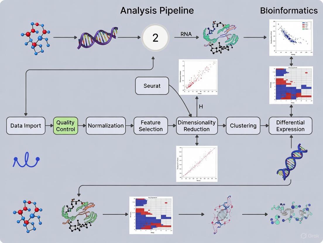
This article provides researchers, scientists, and drug development professionals with a complete framework for implementing a single-cell RNA-seq analysis pipeline using the Seurat toolkit.
A Comprehensive Guide to Building a Robust Single-Cell RNA-Seq Analysis Pipeline with Seurat
Abstract
This article provides researchers, scientists, and drug development professionals with a complete framework for implementing a single-cell RNA-seq analysis pipeline using the Seurat toolkit. Covering the entire workflow from foundational quality control and data exploration to advanced integration techniques and spatial transcriptomics, it offers practical, step-by-step guidance. The content also addresses critical troubleshooting for large-scale projects and benchmarking for method validation, empowering users to generate biologically insightful and reproducible results for biomedical and clinical research.
Laying the Groundwork: Quality Control, Normalization, and Initial Clustering
Setting Up the Seurat Object and Understanding Count Matrix Structure
In single-cell RNA sequencing (scRNA-seq) analysis, the count matrix represents the fundamental data structure from which all subsequent biological insights are derived. This matrix quantifies gene expression at the single-cell level, where each entry contains the number of RNA molecules originating from a specific gene within an individual cell [1]. The precise construction and interpretation of this matrix is therefore a critical first step in any scRNA-seq analysis pipeline.
Depending on the library preparation method used, sequencing reads can be derived from either the 3' ends of transcripts (10X Genomics, Drop-seq, inDrops) or from full-length transcripts (Smart-seq2) [2]. For the increasingly popular 3' end sequencing methods used in droplet-based platforms, the resulting data incorporates unique molecular identifiers (UMIs) that enable distinction between biological duplicates and technical amplification duplicates [2]. This technical consideration directly influences how the count matrix is constructed and interpreted.
The Seurat package for R provides a comprehensive toolkit for scRNA-seq analysis, with the Seurat object serving as a centralized container that integrates both raw data (like the count matrix) and analytical results (such as clustering or differential expression) [3] [4]. Establishing a properly formatted Seurat object with correctly interpreted count data establishes the foundation for all downstream analyses including cell clustering, marker identification, and trajectory inference.
Composition and Generation of the Count Matrix
Fundamental Components
A scRNA-seq count matrix is structured with genes as rows and cells as columns, where each value represents the expression level of a particular gene in a specific cell [5]. For droplet-based methods employing UMIs, these values typically represent the number of deduplicated UMIs mapped to each gene, providing a digital measure of gene expression that is resistant to PCR amplification biases [2].
The generation of a count matrix from raw sequencing data requires several processing steps that vary depending on the experimental protocol. For 10X Genomics data, the Cell Ranger software suite provides a customized pipeline that aligns reads to the reference genome using STAR and counts UMIs per gene [5]. Alternative approaches include pseudo-alignment methods such as alevin, which can process data more quickly by avoiding explicit alignment [5]. For other multiplexed protocols, more generalized tools like scPipe can process the data using the Rsubread aligner [5].
Key Information Elements
The construction of a proper count matrix relies on several crucial information components extracted from the sequencing data [2]:
- Cellular barcode: A unique nucleotide sequence that identifies which cell each read originated from
- Unique molecular identifier (UMI): A random nucleotide sequence that distinguishes individual mRNA molecules, enabling PCR duplicate removal
- Gene identifier: The specific gene transcript from which the read originated
Table 1: Essential Components of scRNA-seq Sequencing Data
| Component | Function | Example |
|---|---|---|
| Cellular Barcode | Identifies cell of origin | 10X Chromium: 16 nucleotides |
| UMI | Identifies individual molecules | 10-12 random nucleotides |
| Gene Identifier | Maps reads to genes | ENSG00000139618 (BRCA2) |
These components are protocol-specific. For example, in 10X Genomics data, the cellular barcode and UMI are contained in Read 1, while the gene sequence is in Read 2. For inDrops v3, this information is distributed across four separate reads [2].
From Sequencing to Count Matrix
The transformation of raw sequencing data into a count matrix follows a standardized workflow regardless of the specific droplet-based method used [2]. After obtaining FASTQ files from the sequencing facility, the process involves:
- Read formatting and barcode filtering: Extracting cellular barcodes and UMIs, then filtering out low-quality barcodes
- Sample demultiplexing: Separating reads from different samples using sample barcodes
- Mapping/pseudo-mapping: Aligning reads to a reference genome or transcriptome
- UMI collapsing and quantification: Removing PCR duplicates and generating final counts per gene per cell
This process yields the final count matrix where each value represents the number of deduplicated UMIs (or reads for full-length protocols) mapped to each gene in each cell [2].
Creating the Seurat Object
Reading in Count Data
The first step in Seurat analysis is importing the count matrix into R and creating a Seurat object. For data processed through the 10X Genomics pipeline, Seurat provides the Read10X() function, which reads the output directory of Cell Ranger and returns a UMI count matrix [3]. This matrix can then be used to create a Seurat object:
The CreateSeuratObject() function requires the count matrix as its primary input, with cells as columns and features (genes) as rows [6]. Key parameters include min.cells, which filters out genes detected in fewer than this number of cells, and min.features, which filters out cells containing fewer than this number of detected genes [6].
Structure of the Seurat Object
The Seurat object employs an organized structure to store various types of data throughout the analysis workflow [7]. Key components include:
- Assays: Container for expression data (e.g., RNA, SCT), with slots for raw counts, normalized data, and scaled data
- meta.data: Data frame storing cell-level metadata including QC metrics
- reductions: Dimensionality reductions (PCA, UMAP, etc.)
- graphs: Nearest neighbor graphs used for clustering
- active.ident: Current cell identity classes
Table 2: Key Slots in the Seurat Object
| Slot | Contents | Access Method |
|---|---|---|
| assays | Expression data (counts, normalized data) | pbmc[["RNA"]] |
| meta.data | Cell-level metadata | pbmc@meta.data or pbmc$nFeature_RNA |
| reductions | Dimensionality reductions | pbmc[["pca"]] |
| active.ident | Current cell identities | Idents(pbmc) |
| graphs | Neighbor graphs for clustering | pbmc[["RNA_nn"]] |
Upon creation, the Seurat object automatically computes and stores basic QC metrics in the meta.data slot, including nCount_RNA (total UMIs per cell) and nFeature_RNA (number of genes detected per cell) [3] [4]. These metrics form the basis for subsequent quality control steps.
Quality Control and Count Matrix Filtering
QC Metrics Calculation
After creating the Seurat object, additional QC metrics should be calculated to identify potentially problematic cells. A particularly important metric is the percentage of mitochondrial reads, which serves as an indicator of cell viability [3] [4]. This can be calculated and added to the object metadata using:
The mitochondrial percentage is biologically informative because low-quality or dying cells often exhibit extensive mitochondrial contamination due to impaired membrane integrity [3]. Similarly, unusually high or low numbers of detected genes can indicate doublets/multiplets or low-quality cells respectively [4].
Data Filtering Thresholds
Appropriate filtering thresholds depend on the biological system and technology used, but general guidelines exist. Typical approaches include [3] [1]:
- Filtering cells with unique gene counts outside expected ranges (typically 200-2,500 for standard 10X protocols)
- Removing cells with excessively high mitochondrial content (often >5-15%)
- Eliminating genes detected in very few cells (default min.cells = 3 in Seurat)
Table 3: Standard QC Thresholds for scRNA-seq Data
| QC Metric | Typical Threshold | Biological Interpretation |
|---|---|---|
| nFeature_RNA (lower bound) | 200-500 | Removes empty droplets/low-quality cells |
| nFeature_RNA (upper bound) | 2,500-5,000 | Removes doublets/multiplets |
| percent.mt | 5-15% | Removes dying/low viability cells |
| min.cells | 3 | Removes rarely detected genes |
These thresholds can be visualized using violin plots or scatterplots to identify appropriate cutoffs before applying them with the subset() function [3]:
Table 4: Key Research Reagent Solutions for scRNA-seq Analysis
| Resource | Function | Application Context |
|---|---|---|
| Cell Ranger (10X Genomics) | Processing raw sequencing data to count matrix | 10X Genomics library preparations |
| STARsolo | Alignment and quantification of scRNA-seq data | Alternative to Cell Ranger, faster processing |
| Seurat Package | Comprehensive scRNA-seq analysis platform | Primary tool for downstream analysis |
| GENCODE Annotation | Comprehensive gene annotation reference | Improved read assignment versus RefSeq |
| UCSC/Ensembl Genome Browser | Reference genome sequences | Essential for read alignment |
| bcl2fastq | Conversion of BCL to FASTQ format | Processing raw sequencing output |
| DoubletFinder/scds | Doublet detection algorithms | Identifying multiplets in droplet data |
Count Matrix Characteristics and Storage
Sparse Matrix Representation
scRNA-seq data is characterized by an abundance of zero values, as each individual cell expresses only a fraction of the total transcriptome. This sparsity makes efficient storage crucial for managing computational resources [3]. Seurat automatically uses sparse matrix representations whenever possible, resulting in significant memory savings:
In typical analyses, sparse matrix representations can reduce memory usage by 20-fold or more compared to dense matrices [3]. This efficiency becomes increasingly important as dataset sizes grow into the tens or hundreds of thousands of cells.
Count Matrix Inspection
Direct examination of the count matrix can provide valuable insights into data quality and structure. Seurat enables focused inspection of specific genes across subsets of cells [3]:
This examination typically reveals the sparse nature of the data, with most entries represented as zeros (indicated by "." in the output) [3]. Understanding this sparsity is essential for selecting appropriate analytical approaches in downstream steps.
The creation of a properly structured Seurat object and thorough understanding of count matrix composition establish the critical foundation for any successful single-cell RNA sequencing analysis. The count matrix, with genes as rows and cells as columns, encapsulates the essential gene expression information extracted through specialized processing of raw sequencing data [2] [5]. Implementation of appropriate quality control measures, including filtering based on detected gene counts and mitochondrial percentage, ensures that downstream analyses reflect biological reality rather than technical artifacts [3] [1].
The structured organization of the Seurat object provides an efficient framework for maintaining data integrity throughout the analytical workflow, seamlessly integrating raw counts, normalized values, cell metadata, and analytical results [7]. By establishing this robust foundation during the initial phases of analysis, researchers position themselves to extract biologically meaningful insights from their single-cell data through subsequent clustering, differential expression, and trajectory analysis procedures.
Within the framework of establishing a robust single-cell RNA sequencing (scRNA-seq) analysis pipeline using Seurat, quality control (QC) represents a critical first computational step. The primary goals of QC are to filter the data to retain only high-quality, genuine cells and to identify any failed samples, thereby ensuring that subsequent analyses like clustering accurately reflect distinct biological cell type populations rather than technical artifacts [8]. This process is challenging because it requires distinguishing between poor-quality cells and biologically relevant but less complex cell types, all while choosing appropriate filtering thresholds to avoid discarding valuable biological information [8] [9]. This protocol outlines a comprehensive methodology for assessing cell quality based on three cornerstone metrics: the number of detected genes per cell (nFeature_RNA), the total number of UMIs per cell (nCount_RNA), and the percentage of reads mapping to the mitochondrial genome (percent.mt).
Key Quality Control Metrics and Their Biological Interpretation
The following table summarizes the core QC metrics used for filtering cells in a scRNA-seq experiment, detailing their technical interpretations and biological significance.
Table 1: Key QC Metrics for Single-Cell RNA Sequencing Data
| Metric | Description | Indication of Low Quality | Biological Consideration |
|---|---|---|---|
nFeature_RNA |
Number of unique genes detected per cell [3]. | Very few genes: empty droplets or heavily degraded cells [3] [10]. | Low complexity can be a genuine feature of quiescent cell populations or small cells [10]. |
nCount_RNA |
Total number of RNA molecules (UMIs) detected per cell [3]. | Low counts: ambient RNA or non-cell entities [10]. | Cells with high counts may be larger or metabolically active; extreme highs can suggest multiplets [8] [3]. |
percent.mt |
Percentage of mitochondrial transcript counts per cell [3]. | High percentage: cellular stress, apoptosis, or broken membranes [3] [10]. | Certain cell types involved in respiration may naturally have higher mitochondrial activity [10]. |
The interplay of these metrics is crucial for accurate QC decision-making. As visually summarized in the workflow below, the process involves calculating these metrics, performing a joint assessment through visualization, and applying informed thresholds to remove low-quality cells.
Materials and Methods
Research Reagent Solutions
The following reagents and computational tools are essential for executing the QC workflow described in this protocol.
Table 2: Essential Research Reagents and Tools for scRNA-seq QC
| Item | Function / Description | Example / Note |
|---|---|---|
| Cell Ranger | Software suite for processing raw sequencing data from 10X Genomics assays into a count matrix [9]. | Version 7.0+ incorporates intronic reads in UMI counting by default [9]. |
| Seurat R Package | Comprehensive toolkit for the loading, processing, analysis, and exploration of scRNA-seq data [3] [10]. | The central environment for executing the entire QC protocol. |
| Loupe Browser | 10X Genomics' visual software for preliminary data exploration and cell filtering [9]. | Provides an intuitive interface for visual QC with real-time feedback [9]. |
| Mitochondrial Gene Set | A predefined set of genes used to calculate the percentage of mitochondrial reads. | Pattern is species-specific: "^MT-" for human, "^mt-" for mouse [3] [10]. |
Experimental Protocol: A Step-by-Step Guide
Step 1: Calculation of QC Metrics
After initializing a Seurat object, the first step is to compute the key QC metrics, including the mitochondrial percentage.
Code Chunk 1: Calculating Mitochondrial Percentage and Metadata Preparation
Step 2: Visualization and Joint Assessment of QC Metrics
Visualization is critical for understanding the distributions of QC metrics and their correlations, which informs the setting of appropriate thresholds.
Code Chunk 2: Generating Multi-Metric QC Plots
The following diagram illustrates the decision-making logic for interpreting these visualizations and identifying cells that should be filtered out.
Step 3: Application of Filtering Thresholds
Based on the visual assessment, filter the Seurat object to retain only high-quality cells. The following table provides common starting thresholds, which must be tailored to the specific biological context of the experiment [3] [10].
Table 3: Example Thresholds for Cell Filtering
| Metric | Typical Lower Bound | Typical Upper Bound | Rationale |
|---|---|---|---|
nFeature_RNA |
200 - 500 [3] [10] | 2000 - 6000 (dataset-dependent) | Removes empty droplets and filters potential multiplets. |
nCount_RNA |
500 - 1000 [8] [10] | Typically derived in correlation with nFeature_RNA |
Filters cells with low sequencing depth. |
percent.mt |
- | 5% - 20% (biology-dependent) [3] [10] | Removes stressed, dying, or low-quality cells. |
Code Chunk 3: Filtering the Seurat Object
Discussion
Implementing rigorous quality control is a foundational step in any scRNA-seq analysis pipeline. The protocol described here leverages the Seurat package to filter cells based on three cardinal metrics, providing a balance between removing technical artifacts and preserving biological heterogeneity. A key consideration is that thresholds are not universal; they must be informed by the biological context. For instance, thresholds for nFeature_RNA and nCount_RNA can vary significantly based on the cell capture technology and the sequencing depth [8] [11], while the cutoff for percent.mt must be adjusted if the biological sample contains inherently high mitochondrial activity, such as in metabolically active tissues [10].
Furthermore, researchers should be aware that current best practices recommend a more permissive approach to filtering, as overly aggressive thresholds can lead to the loss of rare but biologically genuine cell populations [10]. While this protocol focuses on standard metrics, the field is evolving with dedicated tools for addressing specific challenges like doublet detection (e.g., Scrublet, DoubletFinder) and ambient RNA removal (e.g., SoupX) [8] [10], which can be integrated for a more sophisticated QC pipeline. Ultimately, the decisions made at this initial stage profoundly impact all downstream analyses, from dimensionality reduction and clustering to the final biological interpretations, making careful and documented QC an indispensable component of reproducible single-cell research.
In the analysis of single-cell RNA sequencing (scRNA-seq) data, normalization is a critical preprocessing step designed to remove technical variability, such as differences in sequencing depth between cells, thereby enabling meaningful biological comparisons [12]. Without effective normalization, technical artifacts can confound biological signals, severely impacting downstream analyses like clustering, dimensional reduction, and differential expression [12]. Within the widely used Seurat toolkit, two primary normalization methodologies are employed: the conventional LogNormalize approach and the more recently developed SCTransform (Single-Cell Transform) [13] [3] [14]. This article provides detailed application notes and protocols for implementing these strategies within a robust single-cell RNA-seq analysis pipeline, framed for researchers and drug development professionals.
The fundamental challenge addressed by normalization is the heteroskedasticity of count data, where the variance of a gene's counts depends strongly on its mean expression level [15]. Technical factors, most notably varying sequencing depths (total UMIs per cell), can create differences in observed counts that are not reflective of true biological states [13] [12]. The goal of any normalization procedure is to mitigate these technical effects while preserving and highlighting the biological heterogeneity of interest.
Theoretical Foundations and Mathematical Frameworks
The LogNormalize Method
The LogNormalize method, often referred to as global-scaling normalization, operates on a relatively straightforward principle. It normalizes the feature expression measurements for each cell by the total expression for that cell, multiplies this by a scale factor (defaulting to 10,000), and then log-transforms the result [3]. This process can be summarized by the following equation for a count ( y_{gc} ) of gene ( g ) in cell ( c ):
[ \text{Normalized Expression} = \ln\left( \frac{y{gc}}{\sum{g} y_{gc}} \times \text{scale.factor} + 1 \right) ]
The addition of 1 (a pseudo-count) prevents taking the logarithm of zero. This method implicitly assumes that each cell was originally expected to contain the same number of RNA molecules—an assumption that does not always hold true in real-world single-cell experiments [3] [14]. Following normalization, the data is typically scaled (a z-score transformation) such that the mean expression across cells is 0 and the variance is 1 for each gene, giving equal weight to all genes in downstream analyses [3] [16].
The SCTransform Method
SCTransform represents a significant methodological advancement by using a regularized negative binomial regression model to simultaneously normalize data, stabilize variance, and identify variable features [13] [14] [16]. It directly models the UMI counts using a gamma-Poisson (negative binomial) distribution to account for the overdispersed nature of single-cell data. The core of the method involves calculating Pearson residuals for each gene in each cell:
[ r{gc} = \frac{y{gc} - \hat{\mu}{gc}}{\sqrt{\hat{\mu}{gc} + \hat{\alpha}{g} \hat{\mu}{gc}^2}} ]
Here, ( \hat{\mu}{gc} ) is the expected count based on the model, and ( \hat{\alpha}{g} ) is the estimated dispersion parameter for gene ( g ) [15] [16]. These residuals, which represent normalized expression values, are variance-stabilized—meaning they have approximately constant variance across the dynamic range of expression levels—making them suitable for downstream statistical analyses [13] [16]. A key advantage of this approach is its ability to account for the strong relationship between a gene's mean expression and its variance, which simpler methods like LogNormalize do not adequately address [15] [16].
Table 1: Core Mathematical Principles of Each Normalization Method
| Feature | LogNormalize | SCTransform |
|---|---|---|
| Underlying Model | Heuristic scaling | Regularized Negative Binomial |
| Transformation | Log with pseudo-count | Pearson Residuals |
| Variance Stabilization | Limited | Explicitly modeled |
| Handling of Overdispersion | No | Yes |
| Technical Noise Modeling | Basic (library size only) | Comprehensive |
Comparative Performance Analysis
Analytical Benchmarks
When comparing the performance of these normalization methods, several key differences emerge. SCTransform consistently demonstrates superior performance in handling the mean-variance relationship inherent in single-cell data, effectively reducing technical artifacts while preserving biological heterogeneity [13] [15]. In practical benchmarks, SCTransform has been shown to reveal sharper biological distinctions between cell subtypes compared to the standard LogNormalize workflow [13]. For instance, analysis of PBMC datasets normalized with SCTransform typically shows clearer separation of CD8 T cell populations (naive, memory, effector) and additional developmental substructure in B cell clusters [13].
A significant advantage of SCTransform is its ability to mitigate the influence of sequencing depth variation on higher principal components. Whereas log-normalized data often shows persistent confounding effects of sequencing depth, sctransform substantially removes this technical variation, enabling the use of more principal components in downstream analyses that may capture subtle biological signals [13]. Furthermore, SCTransform automatically identifies a larger set of variable features (3,000 by default versus 2,000 for LogNormalize), with these additional features being less driven by technical differences and more likely to represent meaningful biological fluctuations [13].
Practical Implementation Considerations
Table 2: Practical Comparison for Pipeline Implementation
| Aspect | LogNormalize | SCTransform |
|---|---|---|
| Workflow Steps | NormalizeData(), FindVariableFeatures(), ScaleData() | Single SCTransform() command |
| Computation Time | Faster | Slower but more comprehensive |
| Data Output | Normalized counts in RNA@data |
Residuals in SCT@scale.data |
| Downstream Compatibility | Standard Seurat workflow | Compatible with most Seurat functions |
| Integration Performance | Requires separate integration steps | Excellent for integration workflows |
| Confounding Factor Regression | Manual during scaling | Built-in vars.to.regress parameter |
From an implementation perspective, SCTransform offers a more streamlined workflow by replacing three separate commands—NormalizeData(), FindVariableFeatures(), and ScaleData()—with a single function call [13] [14]. This consolidation reduces the potential for user error and ensures consistency in the preprocessing steps. Additionally, SCTransform includes a built-in capability to regress out unwanted sources of variation, such as mitochondrial percentage or cell cycle effects, during the normalization process itself [13] [14].
Experimental Protocols and Application Notes
Protocol 1: LogNormalize Workflow Implementation
The following step-by-step protocol details the implementation of the standard LogNormalize workflow within Seurat:
Quality Control and Filtering: Begin by removing low-quality cells based on QC metrics. Typical thresholds include filtering cells with unique gene counts (nFeature_RNA) outside the 200-2,500 range and mitochondrial percentage (percent.mt) below 5% [3].
Normalization: Apply the LogNormalize method with default parameters.
Variable Feature Identification: Select the top 2,000 most variable genes for downstream analysis.
Scaling and Confounding Factor Regression: Scale the data and optionally regress out unwanted sources of variation such as mitochondrial percentage.
Proceed to Downstream Analysis: The normalized and scaled data is now ready for dimensional reduction (PCA, UMAP) and clustering [3].
Protocol 2: SCTransform Workflow Implementation
The following protocol outlines the implementation of the SCTransform workflow, which replaces multiple steps of the conventional approach:
Quality Control and Filtering: Apply the same QC filtering criteria as in Protocol 1.
SCTransform Normalization: Perform normalization, variance stabilization, and variable feature identification in a single step, with optional regression of mitochondrial percentage.
Note: During normalization, SCTransform automatically accounts for sequencing depth. The
vars.to.regressparameter can be used to simultaneously remove other unwanted sources of variation [13] [14].Proceed to Downstream Analysis: The transformed data is stored in the "SCT" assay, which is automatically set as the default for subsequent analyses.
Protocol 3: Integration of Multiple Samples with SCTransform
For studies involving multiple samples or conditions, SCTransform provides a powerful approach for data integration:
Split Object by Sample: Divide the Seurat object by the sample identifier.
Independent SCTransform: Apply SCTransform independently to each sample.
Select Integration Features: Identify features that are variable across all datasets.
Prepare Data for Integration: Run the PrepSCTIntegration command.
Identify Anchors and Integrate: Find integration anchors and perform the actual integration.
Downstream Analysis: Run dimensional reduction and clustering on the integrated data.
Visualization of Methodologies and Workflows
Normalization Method Conceptual Diagram
Diagram 1: Comparative Workflows of LogNormalize and SCTransform Methods. The diagram illustrates the sequential steps in each normalization approach, highlighting the more integrated nature of SCTransform.
Data Transformation Pathway
Diagram 2: Data Transformation Pathways. This diagram contrasts how each method processes challenging aspects of single-cell data, with SCTransform providing more comprehensive handling of technical artifacts.
Table 3: Key Research Reagent Solutions for scRNA-seq Normalization
| Resource Type | Specific Tool/Function | Application Context | Implementation Notes |
|---|---|---|---|
| Computational Framework | Seurat R Package | Overall analysis environment | Required for both normalization methods |
| Normalization Method | NormalizeData() | LogNormalize workflow | With method = "LogNormalize" |
| Advanced Normalization | SCTransform() | SCTransform workflow | Replaces multiple preprocessing steps |
| Integration Tool | IntegrateLayers() | Multi-sample integration | Works with SCT-normalized data [17] |
| Quality Control Metric | PercentageFeatureSet() | Mitochondrial content calculation | Pattern = "^MT-" for human data |
| Variable Feature Selection | FindVariableFeatures() | LogNormalize workflow | selection.method = "vst" |
| Dimensional Reduction | RunPCA(), RunUMAP() | Downstream analysis | Applies to both methods |
| Visualization | DimPlot(), FeaturePlot() | Result exploration | Group.by parameter for comparisons |
Based on current benchmarks and theoretical considerations, SCTransform generally outperforms LogNormalize in most scRNA-seq analysis scenarios, particularly for complex datasets with significant technical variation or when integrating multiple samples [13] [15] [14]. Its ability to simultaneously normalize data, stabilize variance, and identify variable features through a unified statistical framework represents a substantial advancement over the conventional approach.
However, the LogNormalize method remains valuable for certain applications, particularly for researchers in the early stages of pipeline development or when working with computationally constrained environments. The simpler method may also be preferred when performing direct comparisons with historical datasets processed with conventional normalization approaches.
For drug development professionals and researchers implementing single-cell RNA-seq pipelines, the following strategic recommendations are provided:
- Default to SCTransform for new analyses, particularly when working with multiple samples requiring integration or when analyzing cell populations with subtle biological differences.
- Leverage the Built-in Covariate Regression in SCTransform to simultaneously address confounding factors like mitochondrial percentage during the normalization process itself.
- Validate Key Findings with multiple normalization approaches when investigating critical biological questions, as methodological consistency strengthens conclusions.
- Consult Method-Specific Vignettes for specialized applications, particularly for complex experimental designs involving multiple conditions or time series.
The implementation of appropriate normalization strategies forms the foundation for all subsequent analyses in single-cell RNA sequencing workflows. By selecting the method best suited to their experimental design and research questions, scientists and drug development professionals can ensure that their conclusions are built upon a robust analytical foundation, ultimately leading to more reliable biological insights and therapeutic discoveries.
Identification of Highly Variable Features for Downstream Analysis
Within the framework of a single-cell RNA sequencing (scRNA-seq) analysis pipeline, the identification of Highly Variable Features (HVFs) constitutes a critical computational step that directly influences the resolution of all subsequent biological interpretations. This protocol details the implementation of HVF selection using the Seurat package, a cornerstone tool in modern single-cell genomics. The procedure enables researchers to isolate a subset of genes that exhibit high cell-to-cell variation, effectively filtering out technical noise and highlighting genes likely to be driving meaningful biological heterogeneity. For drug development professionals, this step is particularly vital as it focuses analysis on genes that may define distinct cell states or populations, potentially revealing novel therapeutic targets or biomarkers. The following sections provide a comprehensive guide to the theory, application, and quality control of HVF identification, formatted as standardized application notes for seamless integration into research workflows.
Biological and Technical Rationale
In any scRNA-seq dataset, the majority of genes are either uniformly expressed across cells or detected at levels indistinguishable from technical background noise. Highly variable genes (HVGs), in contrast, demonstrate significant variation in expression across the cell population. This variation can stem from several biologically relevant sources, including:
- Dynamic regulatory processes such as those governing cell differentiation, metabolic states, or cell cycle progression.
- Distinct cellular identities, where genes serve as markers for specific cell lineages or subtypes.
- Responses to external stimuli, including drug treatments or microenvironmental signals.
From a statistical perspective, selecting HVFs enhances the signal-to-noise ratio in downstream dimensional reduction techniques like Principal Component Analysis (PCA). By focusing computational power on features that contain the most biologically relevant information, this step ensures that subsequent clustering and visualization are driven by true cellular heterogeneity rather than technical artifacts or uninformative genes [3] [4].
Workflow Integration and Prerequisites
The identification of HVFs occupies a specific position within the broader scRNA-seq analysis workflow. The following diagram illustrates the complete standard pre-processing workflow, with the HVF identification step highlighted in its critical context.
Prerequisite Steps: HVF identification requires properly normalized data. Prior to this step, researchers must have:
- Completed Quality Control (QC): Removed low-quality cells and potential doublets based on metrics like the number of detected genes per cell (
nFeature_RNA), total molecular counts per cell (nCount_RNA), and the percentage of mitochondrial reads (percent.mt) [3] [4] [18]. - Performed Data Normalization: Adjusted raw counts for systematic technical biases, most commonly using a global-scaling method like
LogNormalize, which normalizes by total cellular expression, multiplies by a scale factor (e.g., 10,000), and log-transforms the result [3].
Computational Methodologies
Seurat provides three distinct algorithms for HVF identification, each with unique statistical foundations and performance characteristics. The choice of method depends on the dataset size, biological question, and computational considerations.
The "vst" Method
The "vst" (variance stabilizing transformation) method is the most sophisticated and generally recommended approach. Its algorithm involves a multi-step procedure to account for the strong mean-variance relationship inherent in count-based sequencing data [19] [20].
The "mean.var.plot" (mvp) Method
The "mean.var.plot" method is a bin-based approach that controls for the expression mean when evaluating dispersion. It functions by:
- Calculating average expression and dispersion (variance-to-mean ratio) for each feature.
- Binning genes into a predefined number (
num.bin, default 20) of groups based on their average expression. - Calculating a z-score for dispersion within each bin to identify genes that are outliers relative to their expression-level peers [19] [20].
The "dispersion" (disp) Method
The "dispersion" method is the simplest and fastest of the three. It directly selects genes with the highest dispersion values, calculated as the variance-to-mean ratio. While computationally efficient, this method does not explicitly control for the relationship between mean expression and dispersion, which can lead to the selection of highly expressed but biologically uninteresting genes [19] [20].
Table 1: Comparison of HVF Selection Methods in Seurat
| Method | Key Function | Primary Advantage | Key Parameter(s) | Recommended Use Case |
|---|---|---|---|---|
vst |
FindVariableFeatures(selection.method = "vst") |
Directly models and removes the mean-variance relationship; most robust. | nfeatures, clip.max, loess.span |
Standard for most datasets; ideal for large or complex datasets. |
mean.var.plot (mvp) |
FindVariableFeatures(selection.method = "mvp") |
Controls for mean via binning and z-scoring; allows explicit cutoffs. | mean.cutoff, dispersion.cutoff |
When user-defined mean/dispersion cutoffs are desired. |
dispersion (disp) |
FindVariableFeatures(selection.method = "disp") |
Computational speed and simplicity. | nfeatures |
For rapid preliminary analysis on smaller datasets. |
Step-by-Step Protocol
This section provides a detailed, executable protocol for identifying HVFs in R using Seurat.
Code Implementation
The following code block demonstrates a complete workflow from normalization through HVF identification and visualization, using the "vst" method.
Parameter Optimization and Interpretation
The default parameters in FindVariableFeatures are well-suited for many datasets, but may require optimization for specific applications. The most critical parameters are:
nfeatures: Determines the number of top variable features to select for downstream analysis. The default is 2000. Increasing this number retains more features but can incorporate more noise; decreasing it focuses on the most prominent signals [3] [4].mean.cutoff&dispersion.cutoff: (Forselection.method = "mvp") Allows setting lower and upper bounds on the mean expression and dispersion of selected features. Useful for manually excluding very lowly expressed genes or extremely high outliers [19] [20].clip.max: (Forselection.method = "vst") Sets the maximum value for standardized feature values after variance stabilization. The default'auto'sets this to the square root of the number of cells [19].
Interpreting the Visualization: The plot generated by VariableFeaturePlot and LabelPoints is a mean-variance plot. Genes shown in red are selected as highly variable. The labeled top genes often include known cell-type-specific markers (e.g., CD3D for T cells, MS4A1 for B cells in PBMC data), providing a quick sanity check for the biological validity of the selection [3].
The Scientist's Toolkit
Table 2: Essential Research Reagents and Computational Tools for HVF Analysis
| Item Name | Function / Purpose | Example / Notes |
|---|---|---|
| Seurat Package | Primary software environment for single-cell analysis in R. | Provides the FindVariableFeatures() function. Critical for the entire workflow [3]. |
| Log-Normalized Data | Normalized expression matrix. Required input for HVF detection. | Generated by NormalizeData(). Corrects for library size and transforms data [3] [4]. |
| Variable Feature Plot | Diagnostic visualization. | Verifies HVG selection. Top genes can be labeled for biological validation [3]. |
| Alternative Workflow: SCTransform | A comprehensive normalization and variance stabilization method. | Can replace NormalizeData, FindVariableFeatures, and ScaleData. Uses regularized negative binomial regression [3] [4]. |
Troubleshooting and Quality Control
A successful HVF selection is paramount for the entire downstream analysis. Common issues and their solutions include:
- Too Few/Too Many Variable Features: Adjust the
nfeaturesparameter. If the resulting list is consistently small, inspect the mean-variance plot for unusual distributions and consider relaxing themean.cutoffordispersion.cutoffin the "mvp" method. - Lack of Known Markers in HVF List: If well-established cell type markers for your system are not being selected, it may indicate overly stringent filtering during QC or normalization issues. Revisit the QC metrics and violin plots to ensure a valid cell population is being analyzed.
- Integration Across Batches: For datasets combining multiple samples or conditions, the standard HVF selection performed on a merged object can be confounded by technical batch effects. In such cases, use the
SelectIntegrationFeaturesfunction as part of Seurat's integration workflow, which identifies features that are variable across multiple datasets to improve integration and conserve biological signal while minimizing technical artifacts [17].
Downstream Applications
The set of highly variable features serves as the direct input for several subsequent analytical steps:
- Data Scaling: The
ScaleDatafunction centers and scales the expression values of the HVFs, giving equal weight to all selected genes in downstream dimensionality reduction [3] [4]. - Linear Dimensional Reduction: Principal Component Analysis (PCA) is performed exclusively on the scaled HVF data. These features encapsulate the majority of the biological signal, allowing PCA to effectively reduce data dimensionality while preserving meaningful heterogeneity [3] [4].
- Clustering and Visualization: The principal components generated from HVFs form the basis for graph-based clustering (
FindNeighbors,FindClusters) and non-linear dimensionality reduction for visualization (RunUMAP,RunTSNE). The quality of these results is therefore fundamentally tied to the initial identification of HVFs [3].
The precise identification of Highly Variable Features is a non-negotiable, foundational step in a robust single-cell RNA-seq analysis pipeline using Seurat. The protocols outlined herein provide researchers and drug developers with a standardized framework for executing this task, complete with methodological comparisons, practical code, and quality control measures. By carefully selecting genes that drive cellular heterogeneity, this process ensures that downstream analyses—from population clustering to biomarker discovery—are conducted on a solid foundation of high-confidence biological signal, ultimately leading to more reliable and interpretable scientific conclusions.
Dimensionality Reduction with PCA and Initial Cell Clustering
In the broader context of implementing a single-cell RNA-seq analysis pipeline with Seurat, dimensionality reduction represents a critical computational step that bridges the gap between normalized gene expression data and biological interpretation. Single-cell RNA sequencing (scRNA-seq) generates high-dimensional datasets where each cell is represented by expression levels of thousands of genes, immediately presenting the challenge known as the "curse of dimensionality" [21]. Not all genes are informative for distinguishing cell identities, and the data contains substantial technical noise and redundancy that can obscure biological signals.
Principal Component Analysis (PCA) serves as a fundamental linear dimensionality reduction technique that creates a new set of uncorrelated variables called principal components (PCs) through an orthogonal transformation of the original dataset [21]. These PCs are linear combinations of the original features (genes) ranked by the amount of variance they explain in the data. By focusing on the top principal components, researchers can dramatically reduce data complexity while retaining the most biologically relevant information. This reduction is essential for downstream analyses, including clustering and trajectory inference, as it mitigates noise and computational burden while highlighting meaningful patterns of cellular heterogeneity.
The initial cell clustering that follows PCA leverages these reduced dimensions to group cells based on similar gene expression profiles, effectively partitioning the cellular landscape into putative cell types or states. Within the Seurat ecosystem, this integrated process of dimensionality reduction and clustering forms the backbone of exploratory scRNA-seq analysis, enabling researchers to move from raw expression matrices to biologically meaningful categorizations of cellular diversity.
Theoretical Foundation
The Mathematics of PCA
Principal Component Analysis operates on the fundamental principle of identifying directions of maximum variance in high-dimensional data. Mathematically, given a normalized and scaled gene expression matrix X with dimensions m×n (where m represents cells and n represents genes), PCA seeks to find a set of orthogonal vectors (principal components) that capture the dominant patterns of variation. The first principal component is defined as the linear combination of genes that maximizes the variance:
PC₁ = w₁₁Gene₁ + w₁₂Gene₂ + ... + w₁ₙGeneₙ
where the weights w₁ = (w₁₁, w₁₂, ..., w₁ₙ) are chosen to maximize Var(PC₁) subject to w₁ᵀw₁ = 1. Subsequent components PC₂, PC₃, etc., are defined similarly with the additional constraint that each must be orthogonal to (uncorrelated with) all previous components.
The principal components correspond to the eigenvectors of the covariance matrix of X, and the eigenvalues represent the amount of variance explained by each component. In biological terms, the early PCs that capture the most variance typically represent major sources of cellular heterogeneity, such as distinctions between major cell types, while later PCs with less variance may represent more subtle biological differences or technical noise.
Alternative Dimensionality Reduction Methods
While PCA remains the standard initial dimensionality reduction method for scRNA-seq workflows, several non-linear techniques have gained popularity for visualization and specific applications:
t-Distributed Stochastic Neighbor Embedding (t-SNE): A non-linear graph-based technique that projects high-dimensional data onto 2D or 3D components by defining a Gaussian probability distribution based on high-dimensional Euclidean distances between data points, then recreating the probability distribution in low-dimensional space using Student t-distribution [21]. An independent comparison of 10 different dimensionality reduction methods proposed t-SNE as yielding the best overall performance [21].
Uniform Manifold Approximation and Projection (UMAP): Another graph-based non-linear dimensionality reduction technique that constructs a high-dimensional graph representation of the dataset and optimizes the low-dimensional graph representation to be structurally as similar as possible [21]. UMAP has shown the highest stability and best separation of original cell populations in comparative studies [21].
Boosting Autoencoder (BAE): A recently developed approach that combines unsupervised deep learning for dimensionality reduction with boosting for formalizing structural assumptions [22]. This method selects small sets of genes that explain latent dimensions, providing enhanced interpretability by linking specific patterns in the low-dimensional space to individual explanatory genes.
Table 1: Comparison of Dimensionality Reduction Methods for scRNA-seq Data
| Method | Type | Key Features | Best Use Cases | Limitations |
|---|---|---|---|---|
| PCA | Linear | Computationally efficient, highly interpretable, preserves global structure | Initial dimensionality reduction, large datasets | Limited for capturing complex non-linear relationships |
| t-SNE | Non-linear | Preserves local structure, creates visually distinct clusters | Visualization of cell subpopulations | Computational intensive for large datasets, stochastic results |
| UMAP | Non-linear | Preserves both local and global structure, faster than t-SNE | Visualization, trajectory analysis | Parameter sensitivity, less interpretable than PCA |
| BAE | Non-linear | Incorporates structural assumptions, identifies explanatory gene sets | Pattern discovery in complex systems, temporal data | Computational complexity, newer less-established method |
Experimental Protocol
Pre-processing for Dimensionality Reduction
Before performing dimensionality reduction, proper data pre-processing is essential to ensure meaningful results. The Seurat-guided clustering tutorial outlines this standard workflow [3] [23]:
Quality Control and Cell Filtering: Filter out low-quality cells based on QC metrics including the number of detected genes per cell (nFeatureRNA), total UMI counts per cell (nCountRNA), and percentage of mitochondrial reads (percent.mt). Typical thresholds include removing cells with fewer than 200 detected genes, more than 2,500 detected genes (potential doublets), and more than 5% mitochondrial counts [3].
Normalization: Normalize the feature expression measurements for each cell using the "LogNormalize" method, which normalizes by total expression, multiplies by a scale factor (10,000 by default), and log-transforms the result. The normalized values are stored in
pbmc[["RNA"]]$datain Seurat v5 [3].Feature Selection: Identify highly variable features (genes) that exhibit high cell-to-cell variation using the
FindVariableFeatures()function with the "vst" selection method. By default, 2,000 features are selected for downstream analysis [3].Scaling: Scale the data using the
ScaleData()function to shift the expression of each gene so the mean expression across cells is 0 and scale the expression so the variance is 1. This gives equal weight in downstream analyses, preventing highly-expressed genes from dominating [3]. The results are stored inpbmc[["RNA"]]$scale.data.
PCA Implementation
The core protocol for performing PCA in Seurat consists of the following steps [3]:
Execute PCA: Run PCA on the scaled data using the
RunPCA()function. By default, only the previously identified variable features are used as input.Determine Significant PCs: Identify the number of significant principal components to retain for downstream analyses. While no universal method exists, the following approaches are commonly used:
- Elbow Plot Visualization: Plot the standard deviations of the principal components using
ElbowPlot()to identify an "elbow" point where the explained variance starts to plateau. - Statistical Methods: Use more quantitative approaches such as the JackStraw procedure, though this is computationally intensive.
- Heuristic Thresholds: Commonly, the top 10-50 PCs are selected, capturing the majority of biological variation while excluding technical noise [21].
- Elbow Plot Visualization: Plot the standard deviations of the principal components using
PC Visualization: Explore the PCA results using several visualization techniques:
VizDimLoadings(): Visualize the genes that drive variation in selected principal components.DimPlot(): Plot cells in reduced PCA space, colored by experimental conditions or sample origins.DimHeatmap(): Explore the primary sources of heterogeneity in the dataset by plotting the genes and cells with the strongest positive and negative loadings across multiple PCs.
Initial Cell Clustering
Following dimensionality reduction, cluster cells based on their expression profiles in the reduced PCA space:
Construct Nearest Neighbor Graph: Build a shared nearest neighbor (SNN) graph based on the Euclidean distance in PCA space using the
FindNeighbors()function, specifying the same number of dimensions as selected in the PCA step.Cluster Cells: Perform graph-based clustering using the Louvain algorithm (default) or other methods via the
FindClusters()function. The resolution parameter controls the granularity of clustering, with higher values leading to more clusters.Non-linear Visualization: Project the clustering results into 2D space using non-linear dimensionality reduction methods like UMAP or t-SNE for visualization purposes.
Parameter Optimization
Table 2: Key Parameters for Dimensionality Reduction and Initial Clustering
| Step | Parameter | Default Value | Recommended Range | Effect |
|---|---|---|---|---|
| Feature Selection | nfeatures | 2000 | 1000-3000 | Number of highly variable genes used as PCA input |
| PCA | npcs | 50 | 10-50 | Maximum number of PCs to compute |
| PC Selection | dims | 1:10 | 1:10 to 1:50 | Number of PCs used for downstream clustering |
| Clustering | resolution | 0.8 | 0.4-1.2 | Higher values increase cluster number |
| UMAP | n.neighbors | 30 | 5-50 | Balances local vs. global structure |
Visualization
The following workflow diagram illustrates the complete process of dimensionality reduction and initial cell clustering within the broader scRNA-seq analysis pipeline:
Dimensionality Reduction and Clustering Workflow
The Scientist's Toolkit
Table 3: Essential Research Reagent Solutions for scRNA-seq Dimensionality Reduction and Clustering
| Tool/Software | Function | Application Context | Key Features |
|---|---|---|---|
| Seurat | Comprehensive scRNA-seq analysis | Primary tool for PCA and clustering in R | PCA implementation, graph-based clustering, visualization |
| Scanpy | Scalable scRNA-seq analysis | Python alternative to Seurat | PCA, clustering, visualization, integration with machine learning libraries |
| Harmony | Batch effect correction | Integration of multiple datasets | Projects cells into shared embedding correcting for dataset-specific conditions |
| scran | Scalable scRNA-seq analysis | Low-level processing and normalization | Computes highly variable genes, performs PCA |
| SCTransform | Normalization workflow | Alternative to standard log normalization | Replaces NormalizeData, FindVariableFeatures, ScaleData steps |
| SingleR | Cell type annotation | Automated cell type identification | Uses reference datasets to annotate clusters |
| scType | Cell type identification | Automated cell typing | Uses comprehensive cell marker database for annotation |
Troubleshooting and Optimization
Common Challenges and Solutions
Insufficient Cluster Separation: If clusters appear poorly separated in visualization, consider increasing the number of PCs used (
dimsparameter inFindNeighbors()), adjusting the clustering resolution, or re-evaluating the number of highly variable genes.Over-clustering or Under-clustering: The resolution parameter in
FindClusters()significantly impacts cluster number. Test multiple resolutions (typically 0.4-2.0) and evaluate biological plausibility using known marker genes.Batch Effects: When integrating multiple samples or datasets, batch effects can confound dimensionality reduction. Consider using integration methods such as Harmony, Seurat's CCA integration [17], or the SCTransform normalization workflow with variance stabilization.
Computational Resources: For large datasets (>50,000 cells), PCA can become computationally intensive. Utilize Seurat's support for sparse matrices, consider approximate PCA methods, or utilize tools like Scanorama for extremely large datasets.
Validation and Interpretation
Validating clustering results is essential for biological interpretation:
Differential Expression Analysis: Identify cluster-specific marker genes using
FindAllMarkers()to validate that clusters represent distinct cell populations with unique transcriptional profiles.Annotation with Known Markers: Compare cluster expression profiles with established cell-type markers from literature or databases to assign biological identities.
Conserved Marker Identification: When analyzing multiple conditions, use
FindConservedMarkers()to identify canonical cell type marker genes that are conserved across conditions [17].Cluster Stability: Assess cluster robustness through sub-sampling approaches or by comparing results across different dimensionality reduction methods.
Dimensionality reduction with PCA and initial cell clustering represents a foundational analytical phase in single-cell RNA sequencing analysis that transforms high-dimensional gene expression data into biologically interpretable patterns of cellular heterogeneity. The methodical application of this workflow within the Seurat framework enables researchers to identify distinct cell populations, uncover novel cell states, and form initial hypotheses about cellular function and relationships.
The robustness of this approach lies in its mathematical foundation, which systematically distills the most biologically relevant information from complex transcriptional profiles while mitigating technical noise. When properly implemented with appropriate quality controls and parameter optimization, this analytical sequence serves as a critical gateway to more specialized downstream analyses, including differential expression testing, trajectory inference, and cell-cell communication analysis.
As single-cell technologies continue to evolve, producing increasingly large and complex datasets, the principles of dimensionality reduction and clustering remain essential for extracting meaningful biological insights from the high-dimensional landscape of cellular transcriptomes.
Visualization with UMAP/t-SNE and Exploratory Data Analysis
Single-cell RNA sequencing (scRNA-seq) reveals cellular heterogeneity by profiling transcriptomes of individual cells, generating high-dimensional data where each of the thousands of genes represents a dimension [24]. Analyzing this data requires dimensionality reduction techniques that transform these high-dimensional measurements into lower-dimensional spaces while preserving meaningful biological structure. This process is fundamental for effective visualization and identifying patterns such as cell subpopulations, developmental trajectories, and disease-associated states [25] [26].
Two nonlinear dimensionality reduction methods have become standard in scRNA-seq analysis pipelines: t-Distributed Stochastic Neighbor Embedding (t-SNE) and Uniform Manifold Approximation and Projection (UMAP) [24]. These techniques enable researchers to project high-dimensional single-cell data into two or three dimensions for visualization, facilitating the exploration of complex cellular relationships. Within the Seurat framework, these methods operate downstream of quality control, normalization, and feature selection steps, providing crucial insights into dataset structure that guide subsequent biological interpretation [3] [17].
Table 1: Key Dimensionality Reduction Methods for scRNA-seq Data
| Method | Type | Key Characteristics | Optimization Goal | Best Suited For |
|---|---|---|---|---|
| PCA | Linear | Maximizes variance, orthogonal components | Global covariance structure | Initial feature reduction, noise reduction |
| t-SNE | Nonlinear | Preserves local neighborhoods, exaggerates cluster separation | Local probability distributions | Cluster visualization emphasizing separation |
| UMAP | Nonlinear | Preserves local and more global structure | Topological representation | Cluster visualization with preservation of continuum relationships |
Theoretical Foundations of t-SNE and UMAP
The Evolution from SNE to t-SNE to UMAP
The development of modern dimensionality reduction techniques represents an evolutionary progression from Stochastic Neighbor Embedding (SNE) to t-SNE and finally to UMAP [25]. SNE, the original algorithm, computed probabilities that reflect similarities between data points in both high and low-dimensional spaces using Gaussian neighborhoods [25]. It aimed to minimize the mismatch between these probability distributions using Kullback-Leibler (KL) divergence as a cost function. However, SNE suffered from optimization difficulties and the "crowding problem"—where moderately distant data points became overcrowded in the lower-dimensional representation [25].
t-SNE introduced two critical modifications to address SNE's limitations: symmetrization of the probability distribution and the use of the Student t-Distribution with one degree of freedom for the low-dimensional probabilities [25]. The symmetric approach simplified the gradient computation, significantly improving optimization performance. Meanwhile, the heavier-tailed t-distribution alleviated the crowding problem by allowing moderate distances to be modeled more effectively in the low-dimensional space [25]. These innovations made t-SNE the state-of-the-art method for dimensional reduction visualization for many years.
UMAP builds upon the foundation of t-SNE with theoretical underpinnings in manifold theory and topological data analysis [25]. While sharing conceptual similarities with t-SNE, UMAP employs a different theoretical framework that enables it to preserve more of the global data structure while still capturing local neighborhoods [25] [24]. Algorithmically, UMAP constructs a weighted k-neighbor graph in high dimensions and optimizes the low-dimensional embedding to preserve this graph's topological structure [24].
Mathematical Underpinnings and Comparative Mechanics
The t-SNE algorithm operates through a specific probabilistic framework. First, it computes pairwise similarities between high-dimensional data points, representing them as conditional probabilities ( p{j|i} ) that point ( xi ) would pick point ( x_j ) as its neighbor:
( p{j|i} = \frac{\exp(-||xi - xj||^2 / 2\sigmai^2)}{\sum{k \neq i} \exp(-||xi - xk||^2 / 2\sigmai^2)} )
where ( \sigmai ) is determined through binary search to achieve a user-specified perplexity value, which represents the effective number of local neighbors [25]. t-SNE then symmetrizes these probabilities to create a joint probability distribution: ( p{ij} = \frac{p{j|i} + p{i|j}}{2n} ).
In the low-dimensional space, t-SNE employs a Student t-distribution with one degree of freedom to compute similarities:
( q{ij} = \frac{(1 + ||yi - yj||^2)^{-1}}{\sum{k \neq l} (1 + ||yk - yl||^2)^{-1}} )
The algorithm minimizes the KL divergence between the two probability distributions:
( C = KL(P || Q) = \sumi \sumj p{ij} \log \frac{p{ij}}{q_{ij}} )
This cost function heavily penalizes cases where nearby points in high-dimensional space are mapped far apart in the low-dimensional representation, which causes t-SNE to prioritize preserving local structure over global relationships [25].
UMAP uses a different theoretical approach, defining similarities in high-dimensional space using an exponential kernel:
( p{ij} = \exp(-||xi - xj||^2 / \sigmai) )
where the bandwidth ( \sigma_i ) is determined based on the distance to the k-th nearest neighbor, with k being a user-specified parameter [24]. In the low-dimensional space, UMAP uses a different family of functions:
( q{ij} = (1 + a ||yi - y_j||^{2b})^{-1} )
where a and b are hyperparameters. UMAP then minimizes the cross-entropy between the two fuzzy topological representations:
( C{UMAP} = \sum{i,j} [p{ij} \log \frac{p{ij}}{q{ij}} + (1 - p{ij}) \log \frac{1 - p{ij}}{1 - q{ij}}] )
This symmetric cost function allows UMAP to better preserve both local and global structure compared to t-SNE [25] [24].
Practical Implementation in Seurat Framework
Preprocessing for Dimensionality Reduction
Successful UMAP/t-SNE visualization in Seurat requires meticulous data preprocessing. The standard workflow begins with quality control to remove low-quality cells that could distort the dimensional reduction. Key QC metrics include the number of unique genes detected per cell (nFeatureRNA), total molecules detected per cell (nCountRNA), and the percentage of mitochondrial reads (percent.mt) [3] [18]. Typically, we filter out cells with either anomalously high or low gene counts, and those with elevated mitochondrial percentage (often >5-10% for PBMCs), indicating potential cell stress or apoptosis [3] [27].
Following quality control, data normalization ensures technical variations don't dominate biological signals. Seurat's default approach uses global-scaling normalization ("LogNormalize") that normalizes each cell's feature expression measurements by total expression, multiplies by a scale factor (10,000), and log-transforms the result [3]. The normalized values are stored in pbmc[["RNA"]]$data. Alternatively, the SCTransform() function provides a more advanced normalization approach that can simultaneously account for technical confounding factors [3].
The next critical step is identification of highly variable features—genes that exhibit high cell-to-cell variation, which typically represent biologically meaningful signals rather than technical noise. Seurat's FindVariableFeatures() function selects these features using a variance-stabilizing transformation, typically returning 2,000 genes for downstream analysis [3]. Finally, scaling centers and scales the data so that highly-expressed genes don't dominate the dimensional reduction. The ScaleData() function shifts expression so the mean is 0 and scales variance to 1 across cells, with results stored in pbmc[["RNA"]]$scale.data [3].
Executing UMAP and t-SNE in Seurat
After preprocessing and principal component analysis (PCA), Seurat provides streamlined functions for both UMAP and t-SNE visualization. The standard workflow applies these methods to the principal components that capture the most significant biological variation, rather than directly to the thousands of genes in the original data [3] [17].
For UMAP, the RunUMAP() function generates the embedding:
For t-SNE, the analogous RunTSNE() function creates the embedding:
Both methods typically use the first 20-30 principal components as input, as these capture the most biologically relevant variance while filtering out noise [3] [17]. The resulting embeddings can be colored by cluster identity, experimental condition, expression of specific genes, or other metadata to extract biological insights.
Table 2: Key Parameters for Dimensionality Reduction in Seurat
| Parameter | t-SNE | UMAP | Effect on Output | Recommended Setting |
|---|---|---|---|---|
| Perplexity | ~5-50 [25] | N/A | Balances local/global structure attention | 30 (default) |
| n.neighbors | N/A | ~5-50 [24] | Controls local connectivity vs global structure | 30 (default) |
| Dims | 1:30 [17] | 1:30 [17] | Number of PCs used as input | 10-50 (dataset dependent) |
| Learning Rate | 200 (default) | 1 (default) | Optimization step size | Typically default values |
| Minimum Distance | N/A | 0.3 (default) | Controls cluster compactness | 0.1-0.5 (cluster separation) |
Advanced Applications and Integration Approaches
Multi-Sample Integration with UMAP/t-SNE
When analyzing multiple scRNA-seq datasets—whether from different batches, donors, or experimental conditions—directly applying UMAP or t-SNE to concatenated data can yield misleading visualizations where technical effects dominate biological signals [17]. Seurat's integration workflow addresses this by identifying "anchors" between datasets—pairs of cells from different datasets that are in a matched biological state [17].
The integration process begins by splitting the RNA assay into different layers for each condition:
Next, the IntegrateLayers() function identifies integration anchors and creates a combined dimensional reduction that captures shared biological variance:
After integration, standard UMAP or t-SNE can be applied to the integrated space, yielding visualizations where cells cluster primarily by biological identity rather than technical origin [17]. This enables direct comparison of similar cell states across conditions, facilitating downstream analyses like differential expression and conserved marker identification.
CCP-Assisted Dimensionality Reduction
Recent methodological advances include Correlated Clustering and Projection (CCP), a data-domain approach that serves as an effective preprocessing step for UMAP and t-SNE [24]. CCP operates by partitioning genes into clusters based on their correlations and projecting genes within each cluster into "super-genes" that represent accumulated gene-gene correlations [24].
The CCP-assisted UMAP/t-SNE workflow involves:
- Gene clustering: Partitioning genes into N clusters using k-means or k-medoids based on correlation measures
- Gene projection: Projecting each gene cluster into a single super-gene descriptor using the Flexibility Rigidity Index (FRI)
- Visualization: Applying standard UMAP or t-SNE to the super-gene representation
This approach has demonstrated significant improvements over standard methods, with reported enhancements of 22% in Adjusted Rand Index (ARI), 14% in Normalized Mutual Information (NMI), and 15% in Element-Centric Measure (ECM) for UMAP visualization [24]. Similarly, CCP improves t-SNE by 11% in ARI, 9% in NMI, and 8% in ECM [24]. CCP is particularly valuable for handling low-variance genes that might otherwise be discarded, instead grouping them into a consolidated descriptor that preserves subtle biological signals.
Table 3: Essential Research Reagent Solutions for scRNA-seq Analysis
| Resource | Type | Function | Application Context |
|---|---|---|---|
| Seurat [3] | R Package | Comprehensive scRNA-seq analysis toolkit | Primary framework for data processing, normalization, clustering, and visualization |
| SingleR [18] | R Package | Automated cell type annotation | Reference-based cell type identification using reference transcriptomic datasets |
| celldex [18] | R Package | Reference dataset collection | Provides curated reference datasets for cell type annotation with SingleR |
| scDblFinder [28] | R Package | Doublet detection | Identification and removal of multiplets from single-cell data |
| SoupX [18] [27] | R Package | Ambient RNA correction | Removal of background contamination from free-floating RNA in solution |
| 10X Genomics Cell Ranger [27] | Computational Pipeline | Raw data processing | Alignment, filtering, barcode counting, and initial feature-barcode matrix generation |
| Loupe Browser [27] | Visualization Software | Interactive data exploration | Visualization and preliminary analysis of 10X Genomics single-cell data |
| SCTransform [3] | Normalization Method | Advanced normalization | Improved normalization accounting for technical confounding factors |
Advanced Analytical Techniques: Data Integration, Marker Identification, and Spatial Transcriptomics
Integrating Multiple Datasets with CCA to Overcome Batch Effects
The integration of multiple single-cell RNA sequencing (scRNA-seq) datasets is a standard step in modern bioinformatics pipelines, essential for unlocking new biological insights that cannot be obtained from individual datasets alone. Pooling datasets from different studies enables robust cross-condition comparisons, population-level analyses, and the revelation of evolutionary relationships between cell types [29]. However, the joint analysis of two or more single-cell datasets presents unique challenges, primarily due to the presence of batch effects—systematic technical variations arising from differences in cell isolation protocols, library preparation technologies, sequencing platforms, or handling personnel [30] [31]. These batch effects are inevitable in multi-dataset studies and can confound true biological variation, leading to misinterpretation of results if not properly addressed [31] [32].
Canonical Correlation Analysis (CCA) has emerged as a powerful computational strategy for batch-effect correction, particularly within the widely-used Seurat toolkit. Unlike approaches that aggressively remove all variation between datasets, CCA identifies shared correlation structures across datasets to align them in a common subspace, effectively removing technical artifacts while preserving meaningful biological heterogeneity [33] [32]. This approach is particularly valuable for large-scale "atlas" projects that aim to combine diverse public datasets with substantial technical and biological variation, including samples from multiple organs, developmental stages, and experimental systems [29]. The following sections provide a detailed protocol for implementing CCA-based integration, benchmark its performance against alternative methods, and outline essential reagents for successful implementation.
Comparative Performance of scRNA-seq Batch Correction Methods
Independent benchmarking studies have comprehensively evaluated numerous batch-effect correction methods across diverse integration scenarios. These benchmarks typically assess methods based on both batch correction efficacy (how well technical variations are removed) and biological preservation (how well true cell-type distinctions are maintained). The table below summarizes key findings from a large-scale benchmark of 14 methods across ten datasets:
Table 1: Benchmarking metrics for popular batch-effect correction methods
| Method | Basis of Approach | Batch Correction Efficacy | Biological Preservation | Recommended Use Cases |
|---|---|---|---|---|
| Seurat (CCA) | Canonical Correlation Analysis + Mutual Nearest Neighbors (MNN) anchors | High | High | General purpose; datasets with shared cell types [32] |
| Harmony | Iterative clustering with PCA dimensionality reduction | High | High | First choice due to fast runtime; multiple batches [34] [32] |
| LIGER | Integrative Non-negative Matrix Factorization (NMF) | Medium-High | High | When biological differences between batches are expected [32] |
| scVI | Variational Autoencoder (VAE) | High | High | Very large datasets; atlas-level integration [29] [34] |
| ComBat | Empirical Bayes framework | Medium | Low-Medium | Simple batch adjustments; may not handle scRNA-seq sparsity well [35] [32] |
| fastMNN | Mutual Nearest Neighbors in PCA space | High | Medium-High | Rapid analysis with minimal parameter tuning [32] |
A more recent evaluation of method performance in complex integration scenarios—such as cross-species, organoid-tissue, and single-cell/single-nuclei RNA-seq integrations—reveals that while CCA-based methods generally perform well, advanced deep learning approaches like scVI and scANVI may be preferable for extremely challenging integration tasks with substantial batch effects [29] [34]. However, for most standard applications, CCA-based integration in Seurat provides an excellent balance of performance, interpretability, and computational efficiency.
Table 2: Quantitative performance scores across integration scenarios (higher values indicate better performance)
| Method | Batch Correction (iLISI/LISI) | Cell Type Conservation (NMI/ARI) | Runtime Efficiency | Scalability to Large Datasets |
|---|---|---|---|---|
| Seurat (CCA) | 0.82 | 0.88 | Medium | High [32] |
| Harmony | 0.85 | 0.86 | High | High [32] |
| scVI | 0.80 | 0.85 | Medium (GPU accelerated) | Very High [29] [34] |
| LIGER | 0.78 | 0.89 | Low-Medium | Medium [32] |
Detailed Protocol: CCA-Based Integration Using Seurat
Preparation of Individual Seurat Objects
The initial phase involves processing each dataset independently to ensure proper normalization and identification of variable features prior to integration:
Step 1: Load and Initialize Seurat Objects
Step 2: Quality Control and Filtering Apply standard QC metrics to remove low-quality cells and potential doublets:
Step 3: Normalization and Variable Feature Selection Process each dataset independently using standard Seurat workflow:
Integration Anchors Identification and Dataset Integration
The core integration process involves identifying correspondence points (anchors) between datasets and using these to correct batch effects:
Step 4: Select Features and Find Integration Anchors Identify features consistently variable across datasets and use them to find correspondence anchors:
Step 5: Integrate Datasets Use the identified anchors to create a batch-corrected integrated dataset:
Integrated Analysis and Downstream Applications
After integration, perform a unified analysis on the combined dataset and conduct comparative analyses across conditions:
Step 6: Integrated Analysis Workflow
Step 7: Identify Conserved Cell Type Markers Switch back to the original RNA assay to find markers conserved across conditions:
Step 8: Differential Expression Across Conditions Compare expression profiles between conditions within specific cell types:
Table 3: Key research reagents and computational tools for scRNA-seq integration
| Category | Specific Tool/Resource | Function/Purpose | Implementation |
|---|---|---|---|
| Analysis Framework | Seurat v4+ | Comprehensive toolkit for single-cell analysis, including CCA integration | R package [30] |
| Alternative Methods | Harmony, scVI, LIGER | Alternative integration approaches for specific use cases | R/Python packages [34] [32] |
| Quality Control | scDblFinder, SoupX | Doublet detection and ambient RNA correction | R packages [34] |
| Normalization | SCTransform, LogNormalize | Data normalization and variance stabilization | Seurat functions [30] |
| Visualization | UMAP, t-SNE | Dimensionality reduction for data visualization | Seurat/Scanpy [32] |
| Benchmarking | scIB | Comprehensive integration benchmarking metrics | Python package [34] |
| Data Repository | Single-cell portals (e.g., GEO, CellXGene) | Source of public datasets for method validation | Web resources |
Technical Considerations and Advanced Applications
Addressing Complex Integration Scenarios
More challenging integration tasks—such as cross-species alignment, organoid-to-tissue comparisons, or combining single-cell and single-nuclei RNA-seq data—present additional hurdles. These scenarios often involve both strong technical confounders and legitimate biological differences that must be carefully distinguished [29]. In such cases, recent methodological advances like sysVI (which combines VampPrior and cycle-consistency constraints in a variational autoencoder framework) may offer advantages over standard CCA by improving batch correction while retaining biological signals [29]. However, for most standard applications with shared cell types across datasets, CCA-based integration remains a robust and well-validated approach.
Order-Preserving Considerations in Batch Correction
An important consideration in batch-effect correction is the "order-preserving" property—maintaining the relative rankings of gene expression levels within each batch after correction. While procedural methods like CCA-based integration effectively align datasets, they may alter certain internal correlation structures. Recent methodological developments aim to address this limitation by incorporating monotonic deep learning networks that explicitly preserve expression orderings while removing batch effects [35]. For analyses where maintaining exact expression hierarchies is critical, these emerging approaches may provide complementary value to standard CCA integration.
CCA-based integration represents a powerful and well-established approach for combining multiple scRNA-seq datasets while effectively mitigating batch effects. The protocol outlined herein provides a robust framework for implementation within the Seurat ecosystem, from initial data preprocessing through integrated analysis and biological interpretation. While alternative methods continue to emerge—particularly for handling exceptionally challenging integration scenarios or specialized analytical requirements—CCA maintains its position as a versatile, high-performing, and computationally efficient choice for most research applications. Proper implementation of these integration workflows enables researchers to leverage the full potential of multi-dataset single-cell studies, facilitating discoveries that transcend the limitations of individual experiments.
Identifying Conserved Cell Type Markers Across Conditions with FindConservedMarkers
In single-cell RNA sequencing (scRNA-seq) studies involving multiple conditions, batches, or donors, a fundamental challenge is distinguishing true biological variation from technical artifacts. The FindConservedMarkers() function in Seurat addresses this by identifying robust cell type markers that remain consistent across different experimental conditions. This capability is particularly valuable in drug development and comparative biology, where researchers need to verify that cell identities persist despite treatments or disease states, enabling valid downstream comparative analyses.
Conserved marker identification represents a critical step in scRNA-seq pipelines when working with multi-condition data. Unlike standard differential expression testing that may identify condition-specific changes, this approach focuses on discovering genes that consistently define cell populations regardless of experimental variables. This methodology ensures that cell type annotations remain stable when comparing control versus treated samples, different technological platforms, or multiple patient cohorts.
Theoretical Framework
Purpose and Applications
The FindConservedMarkers() function serves to identify genes that exhibit consistent differential expression patterns for a specific cell cluster across multiple grouping variables (e.g., conditions, batches, or technologies). Unlike FindAllMarkers(), which identifies markers without considering experimental groups, or FindMarkers(), which performs direct comparisons between two specified identities, FindConservedMarkers() specifically tests whether marker genes remain statistically significant across all conditions [36].
This approach is particularly valuable in several research scenarios:
- Multi-condition experiments: When comparing the same tissues under different treatment conditions
- Cross-species analyses: When identifying orthologous cell types despite evolutionary divergence [37]
- Batch effect mitigation: When technical variations might obscure true biological signals
- Drug development: When verifying that cell type identities remain consistent between control and treatment groups
Statistical Underpinnings
The function operates by performing differential expression testing separately within each condition or group defined in the grouping.var parameter [38]. For each group, it compares the specified cluster (ident.1) against all other cells using a statistical test (default Wilcoxon rank sum). The resulting p-values from each group are then combined using meta-analysis methods from the MetaDE R package, with the default being the minimum p-value method (metap::minimump) [39].
This dual-layered approach ensures that only genes showing consistent expression patterns across conditions are identified as conserved markers. The method accounts for the inherent limitation of single-cell data where each cell is treated as a replicate, which can lead to artificially low p-values if not properly controlled [38].
Experimental Design and Setup
Data Preparation Requirements
Proper experimental design is crucial for successful conserved marker identification. Researchers must ensure:
Integrated Data: Datasets from different conditions should be properly integrated using methods like CCA integration [17], Harmony, or SCVI before seeking conserved markers.
Cell Type Identification: Clustering should be performed on the integrated data to identify cell populations that span across conditions.
Metadata Structure: The grouping variable (e.g., "stim", "condition", "batch") must be properly defined in the Seurat object metadata.
Assay Specification: The default assay should be set to "RNA" rather than "integrated" to access the raw counts for differential expression testing [38].
Quality Control Considerations
Prior to conserved marker identification, standard scRNA-seq quality control metrics should be applied:
- Filtering cells with extreme mitochondrial percentages [3] [18]
- Removing potential doublets using tools like Scrublet [18]
- Ensuring sufficient cell numbers per cluster (>3 cells per group) [39]
Computational Methodology
Workflow Implementation
The following diagram illustrates the complete workflow for identifying conserved cell type markers across conditions:
Parameter Optimization
The FindConservedMarkers() function provides several key parameters that require careful optimization:
Table 1: Critical Parameters for FindConservedMarkers()
| Parameter | Default Value | Recommended Setting | Impact on Results |
|---|---|---|---|
ident.1 |
Required | Specific cluster number | Defines target cluster for marker identification |
grouping.var |
Required | Metadata column name | Specifies condition variable (e.g., "stim", "batch") |
logfc.threshold |
0.25 | 0.25-0.58 | Increases stringency for fold-change |
min.pct |
0.1 | 0.25 | Requires markers in larger cell fraction |
min.diff.pct |
-Inf | 0.25 | Ensures expression differences between groups |
only.pos |
FALSE | TRUE | Returns only upregulated markers |
assay |
"RNA" | "RNA" | Uses raw counts rather than integrated data |
Code Implementation
Results Interpretation
Output Analysis
The output of FindConservedMarkers() contains comprehensive statistical information for each potential marker gene:
Table 2: Interpretation of FindConservedMarkers() Output Columns
| Column Name | Description | Interpretation Guidance |
|---|---|---|
[group]_p_val |
Unadjusted p-value per group | Lower values indicate stronger significance |
[group]_avg_log2FC |
Average log2 fold-change per group | Values >0 indicate higher expression in target cluster |
[group]_pct.1 |
Detection percentage in target cluster | Higher values suggest broader expression |
[group]_pct.2 |
Detection percentage in other cells | Larger difference from pct.1 indicates better specificity |
[group]_p_val_adj |
Adjusted p-value per group | Bonferroni correction for multiple testing |
max_pval |
Largest p-value across groups | Indicates worst-performing condition |
minimump_p_val |
Combined p-value | Meta-analysis result across all conditions |
Statistical Interpretation Framework
The following diagram illustrates the statistical decision-making process implemented in FindConservedMarkers():
Practical Interpretation Guidelines
When interpreting results, researchers should consider:
Prioritize High-Confidence Markers: Genes with high average log2 fold change (>0.58), large differences between pct.1 and pct.2 (>25%), and low combined p-values (<0.001) represent the most reliable markers [38].
Evaluate Consistency: Examine whether log2FC values show consistent direction and magnitude across all conditions.
Biological Relevance: Cross-reference identified markers with established literature and databases to verify biological plausibility.
Visual Validation: Use DotPlot() with split.by parameter to visually confirm conserved expression patterns across conditions [17].
Applications in Drug Development
Case Study: IFN-β Stimulated PBMCs
In the interferon-beta stimulated PBMC dataset [17], FindConservedMarkers() successfully identified NK cell markers (GNLY, NKG7, GZMB) that remained consistent between control and stimulated conditions. This allowed researchers to confidently annotate NK cells while separately analyzing stimulation-responsive genes within this population.
Pathway Analysis Integration
Conserved markers can be used as input for pathway enrichment analyses to identify biological processes and signaling pathways that define specific cell identities regardless of experimental conditions. This approach is particularly valuable in drug development for understanding which cellular functions remain stable versus those altered by therapeutic interventions.
Troubleshooting and Optimization
Common Challenges and Solutions
Table 3: Troubleshooting Guide for FindConservedMarkers()
| Challenge | Potential Causes | Solutions |
|---|---|---|
| No significant markers | Overly stringent thresholds | Adjust logfc.threshold, min.pct, min.diff.pct |
| Inconsistent results | Poor data integration | Revisit integration parameters and methods |
| Long computation time | Large datasets | Use faster test methods, subset data |
| Marker not visualizable | Using integrated assay | Set default assay to "RNA" for visualization |
Performance Optimization
For large datasets, consider these optimization strategies:
- Feature Selection: Pre-filter genes to include only highly variable features
- Parallelization: Implement parallel processing for multiple clusters
- Approximate Methods: Use faster statistical tests for initial screening
- Subsetting: Analyze specific cell populations of interest rather than entire datasets
Research Reagent Solutions
Table 4: Essential Research Reagents and Computational Tools
| Resource | Type | Function | Application Context |
|---|---|---|---|
| Seurat R Package | Software Toolkit | Single-cell analysis | Primary platform for conserved marker identification |
| 10X Genomics Chromium | Platform | Single-cell library preparation | Data generation for analysis |
| IFN-β Stimulated PBMC Dataset | Reference Data | Benchmarking and method validation | Positive control for multi-condition analyses |
| Cell Surface Protein Antibodies | Wet-lab Reagents | Experimental validation | Confirm protein-level expression of identified markers |
| Orthologous Marker Groups (OMGs) | Computational Method | Cross-species marker identification | Comparative biology and evolution studies [37] |
| SingleR | Annotation Tool | Cell type identification | Independent verification of cluster annotations |
| scRNA-seq Annotation Databases | Reference Data | Cell type marker databases | Biological context for identified markers |
The FindConservedMarkers() function provides an essential methodological approach for identifying robust cell type markers that persist across experimental conditions. By implementing the protocols and considerations outlined in this document, researchers can enhance the reliability of their cell type annotations in multi-condition single-cell studies. This methodology forms a critical component of rigorous single-cell analysis pipelines, particularly in translational research and drug development where understanding stable cellular identities amidst experimental perturbations is paramount.
The integration of these computational approaches with experimental validation creates a powerful framework for advancing our understanding of cellular biology across diverse conditions and systems. As single-cell technologies continue to evolve, the principles of conserved marker identification will remain fundamental to extracting biologically meaningful insights from complex multi-condition datasets.
Performing Differential Expression Analysis to Uncover Biological Insights
Differential expression (DE) analysis represents a fundamental computational methodology in single-cell RNA sequencing (scRNA-seq) investigations, enabling researchers to identify genes with statistically significant expression changes between distinct biological conditions, cell types, or experimental treatments. When implemented within a comprehensive Seurat-based analytical pipeline, DE analysis transforms complex transcriptional data into biologically interpretable insights regarding disease mechanisms, therapeutic targets, and cellular responses. This methodology serves as a critical bridge between raw sequencing data and meaningful biological discoveries in biomedical research.
The analytical framework described in these Application Notes provides a standardized approach for identifying and validating differentially expressed genes (DEGs), with particular emphasis on proper experimental design, statistical rigor, and biological interpretation. When properly implemented within a Seurat-based scRNA-seq pipeline, DE analysis enables researchers to pinpoint key molecular drivers of pathological processes, identify novel biomarkers for disease diagnosis and prognosis, and discover potential therapeutic targets for drug development.
Methods
Standard Pre-processing Workflow
The foundation of robust differential expression analysis begins with meticulous data pre-processing to ensure accurate biological interpretations. The standard workflow implemented in Seurat encompasses multiple critical stages that transform raw count data into normalized, scaled expression values suitable for statistical testing.
Quality Control and Cell Filtering: Initial processing requires careful quality assessment and filtering based on established QC metrics [3] [4]. These metrics include the number of unique genes detected per cell (nFeatureRNA), total molecules detected per cell (nCountRNA), and the percentage of mitochondrial reads (percent.mt). Low-quality cells or empty droplets typically exhibit few genes, while cell doublets demonstrate aberrantly high gene counts. Elevated mitochondrial percentages often indicate compromised cell viability [18] [4]. Specific threshold values must be determined empirically for each dataset, though commonly applied cutoffs are summarized in Table 1.
Table 1: Standard QC Thresholds for Single-Cell RNA-seq Data
| QC Metric | Description | Typical Threshold | Biological Interpretation |
|---|---|---|---|
| nFeature_RNA | Number of genes detected per cell | 200-2,500 (PBMC) 200-5,000 (general) | Filters low-quality cells and doublets |
| nCount_RNA | Total number of molecules detected per cell | Dataset-dependent | Removes outliers in sequencing depth |
| percent.mt | Percentage of mitochondrial reads | <5-15% | Identifies dying or stressed cells |
Normalization and Scaling: Following quality filtering, normalization addresses technical variability in sequencing depth between cells. The default LogNormalize method in Seurat normalizes gene expression measurements for each cell by the total expression, multiplies by a scale factor (10,000), and log-transforms the result [3]. For advanced users, the SCTransform() method based on regularized negative binomial regression provides superior normalization while simultaneously estimating variance and mitigating the influence of technical confounders [40]. Subsequently, scaling centers expression values so that the mean expression across cells is zero and scales variance to unity, ensuring equal weight in downstream analyses [3] [4].
Highly Variable Feature Selection: Identification of genes exhibiting high cell-to-cell variation focuses subsequent analysis on biologically informative features. The FindVariableFeatures() function in Seurat selects 2,000 highly variable genes by default using a variance-stabilizing transformation approach, effectively highlighting biological signal rather than technical noise [3] [4].
Differential Analysis Protocols
Seurat provides multiple functions for differential expression testing tailored to specific experimental designs and biological questions. The appropriate method selection depends on the nature of comparisons being made and the experimental structure.
Within-Cluster Differential Expression: The FindMarkers() and FindAllMarkers() functions identify differentially expressed genes between cell groups defined through clustering analysis. These functions perform statistical tests comparing gene expression between specified cell identities, typically using a Wilcoxon rank sum test as the default method, though alternatives including bimod, ROC, t, poisson, negbinom, LR, and DESeq2 are available [17].
Cross-Condition Conserved Marker Identification: When analyzing multiple conditions or batches, the FindConservedMarkers() function performs differential expression testing for each dataset/group independently and combines p-values using meta-analysis methods from the MetaDE R package [17]. This approach identifies canonical cell type marker genes that remain statistically significant irrespective of experimental conditions, treatment effects, or batch variations.
Pseudobulk Analysis for Condition-Specific Effects: For identifying cell-type specific responses to experimental conditions, the AggregateExpression() function generates pseudobulk profiles by summing counts across cells within the same cluster and condition [17]. These aggregated profiles enable conventional differential expression analysis methods like DESeq2 or edgeR, which leverage statistical frameworks developed for bulk RNA-seq data while maintaining single-cell resolution of cell type-specific responses.
Differential Expression Testing Parameters: Proper configuration of statistical parameters ensures biologically meaningful and technically robust results. Key considerations include:
- logfc.threshold: Set to 0.25 by default, this parameter filters genes showing minimum log-fold change
- min.pct: Requires a gene to be detected in a minimum fraction of cells in either population (default: 0.1)
- return.thresh: Adjusted p-value threshold for gene inclusion (default: 0.05)
- test.use: Statistical test methodology selection based on data characteristics
Figure 1: Differential Gene Expression Analytical Workflow. The diagram outlines key decision points and methodological pathways for comprehensive differential expression analysis within the Seurat framework.
Results
Interpretation of Differential Expression Results
Differential expression analysis in Seurat generates comprehensive statistical output requiring careful biological interpretation. A typical results table includes both statistical measures and expression metrics for each tested gene, as illustrated in Table 2.
Table 2: Key Metrics in Differential Expression Results
| Metric | Description | Interpretation Guidelines |
|---|---|---|
| avg_log2FC | Average log2 fold-change | Values > 0 indicate upregulation; < 0 indicate downregulation |
| p_val | Unadjusted p-value | Raw significance measure before multiple testing correction |
| pvaladj | Adjusted p-value (Bonferroni) | Significant typically < 0.05 after multiple test correction |
| pct.1 | Percentage of cells expressing gene in group 1 | Helps distinguish broadly expressed vs restricted markers |
| pct.2 | Percentage of cells expressing gene in group 2 | Large differences may indicate specialized functions |
Conserved marker analysis across conditions, as implemented in FindConservedMarkers(), produces separate statistical outputs for each condition group in addition to combined metrics, enabling assessment of marker stability across technical and biological variations [17]. For example, analyzing NK cells across control and stimulated conditions might identify GNLY, NKG7, and GZMB as highly conserved markers with significant p-values in both conditions and minimal combined p-values [17].
Visualization Strategies for Differential Expression Results
Effective visualization represents a critical component of differential expression analysis, enabling intuitive interpretation of complex statistical results and facilitating biological insights.
Volcano Plots: These scatterplots display statistical significance (-log10 p-value) versus magnitude of expression change (log2 fold-change) for all tested genes, enabling simultaneous assessment of effect size and statistical confidence [41]. Volcano plots efficiently identify the most biologically relevant DEGs occupying the upper-right quadrant (high significance, large fold-change).
Heatmaps: Scaled expression heatmaps of top differentially expressed genes across cells or conditions provide intuitive visualization of expression patterns, co-regulated gene clusters, and sample relationships [42]. The DoHeatmap() function in Seurat generates publication-quality representations that contextualize DEGs within broader transcriptional programs.
Dot Plots: The DotPlot() function with split.by parameter visualizes conserved cell type markers across conditions, simultaneously encoding expression level (color intensity) and percentage of cells expressing each gene (dot size) [17]. This visualization efficiently compares marker expression patterns across multiple conditions or cell types.
Feature and Violin Plots: Gene expression visualization across dimensional reduction embeddings (FeaturePlot()) or grouped by cluster/condition (VlnPlot()) provides spatial context and distribution information for candidate DEGs, facilitating assessment of expression specificity and heterogeneity.
Figure 2: Differential Expression Results Visualization Framework. Multiple complementary visualization strategies transform tabular statistical results into biologically interpretible patterns and insights.
Downstream Functional Analysis
Following DEG identification, functional enrichment analysis contextualizes gene lists within established biological knowledge frameworks, transforming statistical results into mechanistic hypotheses.
Gene Set Enrichment Analysis: Overrepresentation testing of DEGs in annotated pathways (KEGG, Reactome), gene ontology terms (biological process, molecular function, cellular component), or custom gene sets identifies biological processes, molecular functions, and cellular components disproportionately represented among differentially expressed genes.
Protein-Protein Interaction Networks: Mapping DEGs onto established protein interaction databases (STRING, BioGRID) identifies densely connected modules and hub genes potentially serving as regulatory master switches or therapeutic targets within disrupted biological systems.
The Scientist's Toolkit
Research Reagent Solutions
Table 3: Essential Computational Tools for Differential Expression Analysis
| Tool/Category | Specific Examples | Function/Purpose |
|---|---|---|
| Differential Expression Packages | Seurat (FindMarkers, FindConservedMarkers), DESeq2, edgeR | Statistical identification of differentially expressed genes with different algorithmic approaches |
| Visualization Tools | ggplot2, bigPint, Seurat (VlnPlot, FeaturePlot, DotPlot) | Visual representation of expression patterns, statistical significance, and result verification |
| Functional Analysis | clusterProfiler, Enrichr, GOrilla, DAVID | Pathway enrichment, gene ontology analysis, and biological interpretation |
| Normalization Methods | LogNormalize, SCTransform, SCnorm | Technical variability correction and data standardization |
| Quality Control Metrics | PercentageFeatureSet, scater, FastQC | Assessment of data quality and identification of potential artifacts |
Implementation Considerations
Experimental Design Factors: Effective differential expression analysis requires careful experimental planning, including sufficient biological replication (typically 3-5 replicates per condition), balanced sample processing to minimize batch effects, and appropriate control groups for valid comparison. Single-cell studies should target adequate cell numbers per condition (typically 1,000-10,000 cells depending on population heterogeneity) to ensure statistical power for detecting meaningful expression differences.
Parameter Optimization: Critical parameters requiring empirical optimization include:
- Clustering resolution affecting cell population definitions
- Fold-change thresholds balancing sensitivity and specificity
- Expression percentage filters mitigating false positives from rarely detected genes
- Multiple testing correction methods controlling false discovery rates
Integration Considerations: When analyzing multiple conditions or batches, integration methods (CCA, Harmony, RPCA) should be applied before differential expression testing to distinguish biological signals from technical artifacts [17]. The integration workflow typically involves splitting layers by condition, identifying integration anchors, and combining datasets into a unified representation that enables robust comparative analysis.
Annotating Cell Clusters Using Canonical Marker Genes
Cell type annotation represents a critical, defining step in the analysis of single-cell RNA sequencing (scRNA-seq) data, bridging computational clustering results with biological meaning. Following unsupervised clustering of cells based on transcriptional profiles, researchers must annotate these computationally-derived clusters with biologically relevant cell type identities [43]. This process enables meaningful interpretation of cellular heterogeneity, facilitates discovery of novel cell states, and provides a foundation for downstream analyses including differential expression, trajectory inference, and cell-cell communication studies [44] [43]. Within the Seurat ecosystem, which provides a comprehensive toolkit for scRNA-seq analysis, cluster annotation predominantly relies on the identification and interpretation of canonical marker genes - genes that exhibit restricted expression patterns specific to particular cell types or states [43]. This protocol outlines a systematic framework for annotating cell clusters using canonical marker genes within the Seurat environment, providing researchers with both fundamental principles and practical implementation strategies to ensure accurate biological interpretation of their single-cell datasets.
Fundamental Principles of Marker Gene-Based Annotation
What Are Canonical Marker Genes?
Canonical marker genes are genes whose expression is characteristic and diagnostic of specific cell types, lineages, or functional states [43]. These genes typically demonstrate highly restricted expression patterns, showing significant enrichment in particular cell populations compared to all other cells in the dataset. The biological basis for marker gene expression stems from cellular differentiation programs that establish and maintain cell type-specific transcriptional networks. From a practical standpoint, effective marker genes for annotation should exhibit both high expression levels (adequate signal for detection) and high specificity (minimal expression in non-target cell types) [43]. Examples include CD3D and CD8A for cytotoxic T cells, MS4A1 (CD20) for B cells, and LYZ for monocytes, among others documented in the scientific literature [43].
Cluster annotation in Seurat typically follows a hierarchical strategy, beginning with broad cell class identification before progressing to finer subtype resolution [43]. Researchers first distinguish major lineages (e.g., immune versus non-immune cells, epithelial versus mesenchymal cells), then progressively resolve subsets within these broader categories (e.g., Naive CD4 T cells versus Memory CD4 T cells within the T lymphocyte lineage). This hierarchical approach mirrors biological organization and helps prevent misannotation that can occur when attempting to directly assign highly specific identities without establishing broader context. The annotation process integrates multiple lines of evidence, including differential expression testing, marker gene knowledge from literature and databases, and visualization techniques to validate putative assignments [43].
Table 1: Common Canonical Marker Genes for Major Immune Cell Types
| Cell Type | Marker Genes | Biological Function |
|---|---|---|
| T Cells | CD3D, CD4, CD8A | T cell receptor complex; coreceptors |
| B Cells | MS4A1 (CD20), CD79A | B cell receptor signaling |
| Monocytes | LYZ, CD14 | Lysosomal function; LPS receptor |
| NK Cells | GNLY, NKG7 | Cytotoxic granule components |
| Dendritic Cells | FCER1A, CLEC10A | Antigen presentation |
| Platelets | PPBP, PF4 | Platelet activation, coagulation |
Experimental and Computational Workflow
Single-Cell RNA-Seq Wet-Lab Procedures
The accuracy of cluster annotation is fundamentally dependent on sample preparation quality, as technical artifacts can obscure biological signals [45] [44]. While this protocol primarily focuses on computational aspects, understanding key wet-lab considerations is essential for proper experimental design and interpretation. Single-cell isolation methods vary by platform and tissue type, with common approaches including fluorescence-activated cell sorting (FACS), magnetic-activated cell sorting, and microfluidic technologies [45]. Each method presents distinct advantages in throughput, viability, and potential introduction of stress responses. For tissues difficult to dissociate into single-cell suspensions (e.g., neuronal tissue), single-nucleus RNA sequencing (snRNA-seq) provides an alternative approach that minimizes dissociation-induced stress genes but captures only nuclear transcripts [45]. Following cell isolation, library preparation typically involves reverse transcription with unique molecular identifiers (UMIs) to correct for amplification biases, followed by cDNA amplification via PCR or in vitro transcription, and finally sequencing library construction [45]. Throughout these steps, maintaining RNA integrity and minimizing technical batch effects is paramount for obtaining high-quality data amenable to accurate annotation.
Computational Preprocessing in Seurat
Proper computational preprocessing establishes the foundation for successful cluster annotation [3]. The standard Seurat workflow begins with quality control to remove damaged cells, doublets, and empty droplets using metrics including unique feature counts, total molecules, and mitochondrial percentage [44] [3]. Following quality filtering, data normalization addresses differences in sequencing depth across cells, typically using a global-scaling "LogNormalize" method or the improved sctransform approach that simultaneously normalizes data and identifies variable features while mitigating technical artifacts [3] [40]. The identification of highly variable features (genes) focuses subsequent analysis on biologically informative genes, after which scaling gives equal weight to all features in downstream dimensional reduction [3]. Principal component analysis (PCA) linear dimensional reduction enables the application of graph-based clustering algorithms that group cells based on transcriptional similarity, ultimately yielding the clusters requiring annotation [3]. Throughout this process, parameter selection (e.g., number of principal components, clustering resolution) should be guided by biological expectations and dataset characteristics.
Figure 1: Computational Preprocessing Workflow for scRNA-seq Data in Seurat
Core Methodology: Marker-Based Annotation in Seurat
Identifying Cluster-Specific Marker Genes
The annotation process begins with systematic identification of genes that distinguish each cluster from all others. Seurat's FindAllMarkers() function performs differential expression testing between each cluster and the remaining cells, returning a ranked list of candidate marker genes for each cluster [43]. The default Wilcoxon rank sum test identifies genes with differential expression between two groups of cells, though alternative tests including bimod, ROC, and t-test are available for specific applications [3]. For each cluster, researchers should examine the top differentially expressed genes based on statistical significance (adjusted p-value) and effect size (average log fold change). A typical approach considers genes with adjusted p-value < 0.05 and log fold change > 0.5 as potential markers, though these thresholds should be adjusted based on dataset size and biological context. The resulting marker lists provide the primary evidence for cluster identity, to be interpreted in conjunction with existing biological knowledge.
Manual Annotation Using Canonical Markers
Manual annotation represents the most widely used approach for assigning cell type identities, requiring researchers to compare cluster-specific marker genes with established canonical markers from literature and databases [43]. This process involves cross-referencing the top differentially expressed genes for each cluster against known cell type-specific markers, such as those summarized in Table 1. For example, a cluster showing strong expression of CD3D, CD8A, and GZMK would be annotated as cytotoxic T cells, while a cluster expressing MS4A1 and CD79A would be identified as B cells [43]. This manual approach benefits from expert biological knowledge and can accommodate tissue-specific or context-dependent markers, but requires substantial domain expertise and may introduce subjectivity [43]. Successful manual annotation typically employs a conservative approach, beginning with high-confidence assignments based on multiple established markers before progressing to more nuanced distinctions between closely related cell states.
Automated and Semi-Automated Annotation Approaches
To increase throughput, standardization, and accessibility, several automated annotation methods have been developed, including the recent demonstration that large language models like GPT-4 can accurately annotate cell types using marker gene information [46]. When evaluated across hundreds of tissue and cell types, GPT-4 generated annotations exhibiting strong concordance with manual annotations, substantially reducing the required effort and expertise [46]. The GPTCelltype R package provides an interface for this functionality, accepting differential gene lists as input and returning suggested cell type labels [46]. Traditional automated approaches include reference-based methods like SingleR and Seurat's label transfer, which project clusters onto annotated reference datasets to infer identities [43]. While these methods offer efficiency advantages, they perform best when high-quality, biologically relevant reference datasets are available, and typically require manual verification to ensure biologically plausible results [46] [43]. In practice, a hybrid approach that uses automated methods to generate initial hypotheses followed by expert manual curation often yields the most robust annotations.
Table 2: Comparison of Cluster Annotation Methods in Seurat
| Method | Principles | Advantages | Limitations |
|---|---|---|---|
| Manual Annotation | Comparison of differential genes with known markers | Expert interpretation; context-aware | Time-consuming; requires expertise |
| Reference-Based Transfer | Projection to annotated reference datasets | Standardized; rapid | Reference quality-dependent |
| GPT-4 Based | Marker gene interpretation by large language model | Broad knowledge base; rapid | Potential "hallucination"; black box |
| Hybrid Approach | Combines automated suggestions with manual curation | Balances efficiency and accuracy | Still requires some expertise |
Visualization Techniques for Annotation Validation
Dimensional Reduction Plots
Visualization represents a critical component of annotation validation, allowing researchers to assess whether computationally assigned labels align with expected biological patterns [47]. Dimensional reduction techniques including UMAP and t-SNE project high-dimensional single-cell data into two dimensions while preserving neighborhood relationships, enabling visual inspection of cluster identities and relationships [43]. Seurat's DimPlot() function visualizes clustering results in these low-dimensional spaces, with options to color points by cluster identity, experimental condition, or other metadata [47]. When overlaid with cluster annotations, these plots allow researchers to verify that assigned labels correspond to distinct, well-separated populations with expected relationships (e.g., closely related immune cell types forming adjacent clusters) [43]. For presentation purposes, LabelClusters() and LabelPoints() functions add clear, automated positioning of cluster labels directly on dimensional reduction plots [47].
Expression Visualization Plots
Visualizing marker gene expression across clusters provides direct evidence supporting or challenging annotation assignments [47]. Seurat offers multiple specialized visualization functions for this purpose, each highlighting different aspects of expression patterns. FeaturePlot() displays feature expression on a dimensional reduction plot, allowing visual assessment of expression specificity and distribution [47]. VlnPlot() generates violin plots showing the probability density of expression across clusters, facilitating comparison of expression levels and distributions [47]. DotPlot() creates a compact visualization displaying both the percentage of cells expressing a gene (dot size) and the average expression level (color intensity) across all clusters [47]. Finally, DoHeatmap() generates grouped heatmaps showing expression patterns of key marker genes across cells from all clusters, revealing both consistent and variable expression patterns [47]. Together, these complementary visualizations enable comprehensive assessment of whether putative marker genes show the expected expression patterns for assigned cell type labels.
Figure 2: Visualization Approaches for Annotation Validation
Advanced Applications and Integration
Troubleshooting Problematic Annotations
Despite methodological advances, annotation challenges frequently arise in practice, particularly for novel cell types, poorly characterized tissues, or technical artifacts. Several common scenarios require specific troubleshooting approaches. When clusters lack clear marker gene signatures or express unexpected gene combinations, consider potential doublets or multiplets—these typically show simultaneous expression of markers from distinct lineages and abnormally high gene counts [44]. For clusters expressing stress response genes or showing high mitochondrial content, examine dissociation protocols and consider implementing more gentle tissue processing or snRNA-seq approaches [45]. When automated and manual annotations conflict, prioritize manual verification using multiple complementary markers and cross-reference with orthogonal datasets when available. For novel cell populations without clear counterparts in existing references, employ conservative terminology (e.g., "unknown immune population expressing X, Y, Z") and consider functional characterization through gene set enrichment or trajectory analysis rather than forcing established labels.
Integration with Spatial Transcriptomics
The rising availability of spatial transcriptomics technologies enables validation of cluster annotations through spatial localization patterns, providing an orthogonal confirmation method [40]. Seurat supports integration between single-cell RNA-seq and spatial transcriptomics datasets, allowing researchers to project cluster annotations onto tissue architecture and verify that assigned cell types localize to biologically appropriate regions [40]. For example, in mouse brain analysis, hippocampal markers should localize to anatomically defined hippocampal regions, while choroid plexus markers should appear in ventricular regions [40]. The SpatialFeaturePlot() and SpatialDimPlot() functions visualize cluster assignments or gene expression directly on tissue sections, enabling direct correlation between transcriptional identity and spatial context [40]. This spatial validation is particularly valuable for confirming rare populations, identifying potential contamination, and building confidence in annotation schemes before proceeding to downstream functional analyses.
The Scientist's Toolkit
Table 3: Essential Research Reagent Solutions for scRNA-seq Cluster Annotation
| Tool/Category | Specific Examples | Primary Function |
|---|---|---|
| Single-Cell Platforms | 10X Genomics, BD Rhapsody | High-throughput single-cell partitioning |
| Analysis Toolkits | Seurat, SingleCellExperiment | Primary computational analysis environment |
| Annotation Databases | CellMarker, PanglaoDB | Compendia of established marker genes |
| Reference Atlases | Human Cell Landscape, Tabula Sapiens | Annotated reference datasets |
| Automated Annotation Tools | SingleR, SCType, GPTCelltype | Algorithmic cell type prediction |
| Visualization Packages | ggplot2, patchwork, dittoSeq | Flexible visualization of results |
Applying Seurat to Analyze Spatial Transcriptomics Data (10x Visium)
Spatial transcriptomics has emerged as a pivotal advancement in biomedical research, enabling the measurement of all gene activity in a tissue sample while preserving the spatial context of where each gene is expressed [48]. Unlike single-cell RNA sequencing (scRNA-seq), which requires tissue dissociation and loses spatial information, spatial transcriptomics allows researchers to visualize molecular changes occurring in situ and piece together complex cause-and-effect relationships within tissue architectures [49]. The 10x Genomics Visium platform represents one of the most widely adopted spatial transcriptomics technologies, capturing gene expression data from tissue sections while simultaneously providing histological context through H&E staining [40].
The Seurat package, an R toolkit originally developed for scRNA-seq analysis, has been extended to support the analysis of spatially-resolved transcriptomics data [40] [50]. Seurat provides a comprehensive framework that spans the entire analytical workflow—from data preprocessing and normalization to advanced integration with single-cell datasets—enabling researchers to uncover spatially-organized biological patterns within tissues. This protocol focuses specifically on implementing Seurat for analyzing 10x Visium data within the broader context of a single-cell RNA-seq analysis pipeline, providing researchers with standardized methodologies for extracting biologically meaningful insights from spatial transcriptomics experiments.
Key Research Reagent Solutions
Table 1: Essential research reagents and computational tools for spatial transcriptomics analysis with Seurat
| Category | Item | Function/Description |
|---|---|---|
| Wet Lab reagents | Visium Spatial Gene Expression Slide & Reagents (10x Genomics) | Captures spatially barcoded RNA sequences from tissue sections |
| Tissue Optimization & Gene Expression Kits (10x Genomics) | Optimizes permeabilization conditions and enables library preparation | |
| H&E Staining reagents | Provides histological context for spatial expression patterns | |
| Computational tools | Seurat R package (≥v3.2) | Primary analytical toolkit for spatial transcriptomics data |
| hdf5r R package | Enables handling of HDF5 file formats used by 10x pipelines | |
| arrow R package | Supports efficient data storage and access for large datasets | |
| Spacexr/RCTD | Enables deconvolution of cell types within spatial spots | |
| Cell2location | Bayesian method for estimating absolute cell type abundance |
Data Preprocessing and Quality Control
Data Loading and Structure
The initial step in the spatial transcriptomics workflow involves loading the Visium data into Seurat. The data output from the Space Ranger pipeline includes three critical components: (1) a spot-by-gene expression matrix, (2) a digital image of the H&E-stained tissue slice, and (3) scaling factors that relate the original high-resolution image to the lower-resolution image used for visualization [40]. These components are integrated into a Seurat object using the Load10X_Spatial() function:
In Seurat, the spatial expression data is stored in the Spatial assay, while the associated image is stored in a dedicated images slot. The image information enables the association of molecular measurements with their physical positions within the tissue architecture [40].
Quality Control and Normalization
Quality assessment begins with visualization of QC metrics, particularly the total molecular counts per spot, which can exhibit substantial heterogeneity in spatial datasets due to both technical factors and biological differences in cell density across tissue regions [40]. For example, in brain tissue, areas depleted of neurons (such as cortical white matter) typically show lower molecular counts:
For normalization, we strongly recommend using SCTransform() rather than standard log-normalization. The SCTransform method builds regularized negative binomial models of gene expression to account for technical artifacts while preserving biological variance. This approach effectively mitigates the influence of technical factors on normalized expression estimates, particularly for highly expressed genes [40]:
Table 2: Key QC metrics and their interpretation for spatial data
| QC Metric | Recommended Threshold | Biological Interpretation |
|---|---|---|
| nCount_Spatial | Dataset-dependent | Low counts may indicate empty spots; high counts may indicate multiple cells |
| nFeature_Spatial | Dataset-dependent | Low features may indicate poor quality spots; high features may indicate multiple cell types |
| Mitochondrial percentage | <5-10% | Higher percentages may indicate stressed or dying cells |
| Spatial count distribution | Visual inspection | Regional variations may reflect actual cellular density differences |
Analytical Workflow and Visualization
Dimensionality Reduction and Clustering
The analytical pipeline for spatial data closely mirrors standard scRNA-seq workflows, with the addition of spatial visualization capabilities. After normalization, the workflow proceeds through dimensionality reduction and clustering:
For newer, higher-resolution Visium HD datasets, we recommend using the sketch-based clustering workflow, which better preserves rare and spatially restricted populations. This approach subsamples the dataset in a way that maintains population diversity, performs clustering on the subsampled cells, then projects these labels back to the full dataset [51]:
Spatial Visualization Techniques
Seurat provides specialized functions for visualizing molecular data in spatial context. SpatialFeaturePlot() extends the standard FeaturePlot() functionality by overlaying gene expression data on top of tissue histology:
Visualization parameters can be adjusted to optimize the balance between molecular and histological information. The pt.size.factor parameter controls spot size, while the alpha parameter adjusts transparency to emphasize spots with higher expression:
For exploring data interactively, Seurat provides interactive plotting capabilities. Setting the interactive parameter to TRUE in either SpatialDimPlot() or SpatialFeaturePlot() opens an interactive Shiny pane where users can hover over spots to view cell identities and expression values [40].
Diagram 1: Spatial transcriptomics analysis workflow with Seurat. The pipeline progresses from data loading through quality control, normalization, clustering, and visualization, culminating in downstream analytical applications.
Integration with Single-Cell RNA-seq Data
Integration Approaches
Integration of spatial data with single-cell RNA-seq datasets significantly enhances the resolution of spatial analyses by enabling the identification of cell types within each spatial spot. Two primary computational approaches exist for this integration: deconvolution methods that estimate cell type proportions within each spot, and mapping approaches that assign the most likely dominant cell type to each spot [52].
Seurat employs a mapping approach through "label transfer" using an anchor-based integration workflow. This method leverages well-annotated scRNA-seq reference datasets to identify corresponding cell types in spatial data:
Multi-modal Integration
With the introduction of Seurat v5, integrative analysis has been enhanced through multi-modal integration capabilities, including "bridge integration" that can integrate diverse data types such as transcriptomic, epigenomic, and proteomic measurements [50]. This approach is particularly valuable for mapping complex cellular identities across technologies:
Diagram 2: Integration of scRNA-seq and spatial data. Reference scRNA-seq data and spatial transcriptomics data are integrated through anchor identification, enabling both cell type mapping and deconvolution approaches.
Downstream Analytical Applications
Identifying Spatially Variable Features
A key advantage of spatial transcriptomics is the ability to identify genes whose expression patterns correlate with spatial location. Seurat offers multiple workflows for this purpose, including differential expression testing based on pre-annotated anatomical regions and computational approaches that detect spatial patterns without prior histological knowledge [40].
Differential expression based on anatomical regions can be performed using the standard FindMarkers() function, with clusters defined either through unsupervised clustering or based on histological annotations:
For more sophisticated spatial pattern detection without predefined regions, methods like BANKSY (Building Aggregates with a Neighborhood Kernel and Spatial Yardstick) can identify spatially-defined tissue domains by considering both the gene expression of each spot and its spatial neighborhood [51].
Interactive Exploration and Analysis
Seurat's interactive visualization capabilities significantly enhance exploratory data analysis. The LinkedDimPlot() function creates linked visualizations between the UMAP representation and tissue image, allowing users to select regions in one view and see the corresponding spots highlighted in the other [40]:
Interactive spatial plots enable real-time parameter adjustment and detailed examination of specific tissue regions:
Table 3: Troubleshooting common issues in spatial data analysis
| Issue | Potential Cause | Solution |
|---|---|---|
| Low correlation with scRNA-seq | Batch effects or biological differences | Adjust normalization parameters or use harmony integration |
| Poor spatial clustering | Over-normalization or incorrect resolution | Adjust SCTransform parameters or clustering resolution |
| Weak spatial patterns | Insufficient sequencing depth or spatial resolution | Filter low-quality spots or use higher-resolution technologies |
| Ambiguous cell type assignments | Poor reference mapping or mixed cell types | Use deconvolution methods instead of label transfer |
This protocol outlines a comprehensive workflow for analyzing 10x Visium spatial transcriptomics data using Seurat, from initial data loading through advanced integration with single-cell references. The standardized methodologies presented enable researchers to leverage the complementary strengths of spatial context and transcriptional profiling, revealing tissue organization principles that would remain hidden with either approach alone.
As spatial technologies continue to evolve, particularly with the advent of higher-resolution platforms like Visium HD, analytical methods must similarly advance. Future developments in spatial transcriptomics will likely focus on improved normalization strategies specifically designed for spatial data, enhanced multi-omic integration capabilities, and computational methods that more effectively leverage spatial information to reconstruct cellular neighborhoods and interaction networks. By implementing the protocols described herein, researchers can establish a robust foundation for spatial transcriptomics analysis within their single-cell genomics pipelines, accelerating discoveries across biomedical research domains including developmental biology, neuroscience, oncology, and immunology.
Identifying Spatially Variable Features and Linking Molecular & Spatial Information
Spatially resolved transcriptomics (SRT) has revolutionized biological research by enabling the precise mapping of gene expression within intact tissue architecture, preserving the spatial context lost in single-cell RNA sequencing (scRNA-seq) dissociations [53] [54]. A central computational challenge in SRT analysis is the identification of spatially variable features (SVGs)—genes whose expression levels exhibit significant and non-random spatial patterns across a tissue sample [55]. Accurately detecting these genes is a critical first step for downstream analyses, including the definition of spatially restricted domains, understanding cellular communication, and uncovering novel biological insights into tissue function and organization [40] [53]. Furthermore, integrating SRT data with accompanying high-resolution histology images presents a powerful opportunity to link molecular profiles with tissue morphology, thereby enhancing the interpretability and accuracy of analysis [53].
This Application Note provides a detailed protocol for identifying spatially variable genes and integrating molecular with spatial information using the Seurat toolkit and other complementary methods, framed within the broader context of a single-cell RNA-seq analysis pipeline. It is designed for researchers, scientists, and drug development professionals who require robust, reproducible methods for analyzing complex spatial transcriptomics data.
Background and Key Concepts
Spatially Variable Genes vs. Highly Variable Genes
It is crucial to distinguish Spatially Variable Genes (SVGs) from the Highly Variable Genes (HVGs) typically identified in scRNA-seq analyses. While HVGs identify genes with high cell-to-cell expression variance within a dissociated cell population, SVGs specifically capture genes whose expression patterns correlate with spatial location in a tissue [55]. A gene can be highly variable without being spatially variable, and vice-versa. SVG detection methods are explicitly designed to leverage the spatial coordinates of sequencing spots or cells, making them essential for understanding tissue architecture.
The Role of Histology Integration
Many current SRT analysis methods rely solely on molecular profiles (gene expression) for tasks like clustering spots into spatial domains. However, paired histology images contain a wealth of information about cellular morphology and tissue structure that is often underutilized [53]. Integrating image profiles—such as cell type abundances derived from AI-reconstructed histology images—with molecular profiles can significantly improve the accuracy and biological interpretability of spatial analyses, leading to more precise domain identification and more meaningful spatially variable gene detection [53].
Computational Tools for Spatial Transcriptomics
A diverse ecosystem of computational tools has been developed to address the unique challenges of SRT data analysis. The table below summarizes key tools relevant to SVG detection and multi-modal data integration.
Table 1: Key Bioinformatics Tools for Spatial Transcriptomics Analysis
| Tool Name | Primary Function | Key Application in Spatial Analysis | Relevance to SVG/Integration |
|---|---|---|---|
| Seurat [40] | Comprehensive scRNA-seq & SRT analysis | Dimensionality reduction, clustering, & visualization of spatial data; includes Moran's I for SVG detection | Core framework for workflow implementation; enables basic SVG discovery |
| iIMPACT [53] | Multi-modal spatial domain identification | Bayesian model integrating cell type abundance (from images) with gene expression for spatial clustering | Enhances domain definition for more biologically relevant SVG detection |
| SpatialScope [54] | Resolution enhancement & data integration | Uses deep generative models to deconvolve spot-level data to single-cell resolution & infer transcriptome-wide expression | Enables SVG detection at single-cell resolution from spot-based data (e.g., 10x Visium) |
| nnSVG [55] | Spatially Variable Gene detection | Scalable method based on nearest-neighbor Gaussian processes | A top-performing, specialized method for accurate SVG identification |
| SPARK/SPARK-X [55] | Spatially Variable Gene detection | Statistical methods using mixed and non-parametric models | Established methods for robust SVG detection |
| Squidpy [56] | Spatial data analysis ecosystem | Spatial neighborhood analysis, ligand-receptor interaction, and spatial clustering | Useful for downstream analysis after SVG discovery |
| Palo [57] | Visualization optimization | Optimizes color palette assignment for spatial plots to improve cluster distinguishability | Aids in the visual interpretation of spatial domains and gene expression patterns |
Protocol: A Multi-Method Workflow for SVG Identification in Seurat
This protocol outlines a comprehensive workflow for identifying spatially variable genes, beginning with data preprocessing in Seurat and proceeding to specialized SVG detection methods.
Data Preprocessing and Normalization in Seurat
Goal: Prepare raw spatial transcriptomics data (e.g., from 10x Visium) for downstream analysis.
Steps:
- Data Loading: Use the
Load10X_Spatial()function to read the output of the spaceranger pipeline. This creates a Seurat object containing the spot-by-gene expression matrix and the associated tissue image [40]. - Quality Control: Assess metrics like
nCount_Spatial(UMIs per spot). Spatial variation in counts can reflect anatomy (e.g., neuron-dense regions having higher counts) rather than just technical noise [40]. - Normalization: Use
SCTransform()(regularized negative binomial regression) for normalization. Avoid standard log-normalization, as it can fail to adequately normalize highly expressed genes in spatial data where molecular counts vary substantially based on tissue anatomy [40].
Benchmarking and Selecting an SVG Detection Method
Goal: Choose an appropriate and effective method for identifying SVGs.
Numerous methods exist for SVG detection, and their performance can vary. A recent large-scale benchmark evaluated eight popular methods (including SpatialDE, SPARK-X, nnSVG, and Moran's I) across 31 datasets [55]. Key findings to guide method selection are summarized below.
Table 2: Benchmarking Results of SVG Detection Methods (Adapted from [55])
| Method | Average Correlation with Gene Expression | Concordance with Other Methods | Practical Considerations |
|---|---|---|---|
| SPARK-X | High (~0.8) | Low to Moderate | Fast; but SVG ranking is highly dependent on mean expression level |
| nnSVG | Moderate (~0.5) | High (with MERINGUE, Moran's I) | Scalable; performance correlates well with mean expression |
| Moran's I (Seurat) | Information Not Provided | High (with nnSVG, MERINGUE) | Readily available within Seurat pipeline |
| SpatialDE | Information Not Provided | Low | Shows high variability across different technologies/datasets |
| Giotto (K-means/Rank) | Moderate (~0.5) | High (with each other) | Uses spatial network enrichment |
Key Recommendations:
- nnSVG is a strong choice due to its scalability and good performance.
- Be aware that different methods can yield strikingly different sets of significant SVGs even when using the same adjusted p-value threshold. The number of SVGs identified by all methods is often very low [55].
- Consider the dependency on mean expression. Methods like SPARK-X that show high correlation may be biased towards selecting highly expressed genes [55].
Implementing SVG Detection using Moran's I in Seurat
Goal: Perform basic SVG detection directly within the Seurat ecosystem.
After preprocessing and clustering, Seurat's FindSpatiallyVariableFeatures() function can identify genes with spatial patterns using methods like Moran's I. Moran's I is a measure of spatial autocorrelation, where a value of +1 indicates perfect positive spatial autocorrelation (clustering), and -1 indicates perfect negative spatial autocorrelation (dispersion) [55].
Protocol Workflow Diagram
The following diagram illustrates the complete multi-method workflow for identifying spatially variable features, from data input to final validation.
Advanced Integration: Linking Molecular and Spatial Information
Integrating Histology Images with iIMPACT
Goal: Improve spatial domain identification by integrating cell-type abundance from histology images with gene expression data.
The iIMPACT method uses a two-stage, Bayesian statistical framework [53]:
Stage 1: Histology-based Spatial Domain Identification
- Input: A spot-by-cell-type abundance matrix (from AI-based nuclei segmentation of histology images) and a low-dimensional representation of normalized gene expression (e.g., from PCA).
- Model: A Bayesian finite mixture model with a Markov Random Field (MRF) prior. The model uses:
- A multinomial sub-component for cell-type abundance.
- A normal sub-component for gene expression.
- The MRF prior encourages neighboring spots to be clustered into the same spatial domain.
- Output: Mutually exclusive histology-based spatial domains and "interactive zones" (spots with uncertain assignment).
Stage 2: Domain-Specific Differentially Expressed Gene (spaDEG) Detection
- Model: A negative binomial regression model is fitted for each gene to test for differential expression between a specific spatial domain and all others.
- Output: A list of spaDEGs with strong biological interpretability.
In a human breast cancer case study, iIMPACT achieved higher accuracy (Adjusted Rand Index = 0.634) in matching pathologist-annotated regions compared to other methods like SpaGCN (ARI=0.520) and BayesSpace (ARI=0.419) [53].
Enhancing Resolution with SpatialScope
Goal: Achieve transcriptome-wide single-cell resolution from spot-based ST data (e.g., 10x Visium) or infer unmeasured genes for image-based data (e.g., MERFISH).
SpatialScope uses deep generative models to integrate scRNA-seq reference data with ST data [54].
For seq-based ST data (e.g., 10x Visium):
- Concept: A spot's expression vector
yis modeled as the sum of expressionsx1, x2, ...from the individual cells it contains, plus noise. - Process: SpatialScope learns the expression distributions of different cell types from a scRNA-seq reference. It then uses a Langevin dynamics sampler to decompose the spot-level expression
yinto single-cell expressionsx1, x2, ...by sampling from the posterior distributionp(X | y, k1, k2, ...)[54]. - Output: Pseudo-cells with single-cell resolution and transcriptome-wide expression at each location, enabling more precise SVG detection and analysis of cellular communication.
Multi-Modal Integration Diagram
The following diagram illustrates the advanced iIMPACT framework for integrating histology and molecular profiles.
Table 3: Key Research Reagent Solutions for Spatial Transcriptomics
| Resource Name | Type | Function in Analysis |
|---|---|---|
| 10x Genomics Visium | Spatial Transcriptomics Platform | Generates whole-transcriptome data from tissue sections on a spatially barcoded array. Provides standard input data for this protocol. |
| Seurat R Toolkit [40] [56] | Software Package | Primary environment for data loading, QC, normalization, basic SVG detection (Moran's I), clustering, and visualization. |
| scRNA-seq Reference Atlas | Data | Annotated single-cell dataset used by integration methods (e.g., SpatialScope, iIMPACT) for cell type decomposition and imputation. |
| AI-Based Nuclei Segmentation Tool (e.g., Hover-Net) [53] | Software Algorithm | Processes histology images to generate cell type abundance maps, a crucial input for the iIMPACT multi-modal integration model. |
| iIMPACT R/Package [53] | Software Package | Implements the Bayesian model for integrating image and molecular profiles to define histology-based spatial domains. |
| SpatialScope Software [54] | Software Package | Enhances spot-based data to single-cell resolution and infers unmeasured genes for targeted panels using deep generative models. |
| nnSVG R Package [55] | Software Package | A specialized, high-performance tool for accurate SVG detection using nearest-neighbor Gaussian processes. |
Solving Real-World Challenges: Performance, Scalability, and Data Transformation
The emergence of single-cell RNA sequencing (scRNA-seq) atlases and multi-study consortia projects has propelled the field into an era of unprecedented data scale. Analyzing 100+ libraries encompassing over 600,000 cells presents unique computational and statistical challenges that exceed the limitations of standard integration workflows. Such massive datasets introduce substantial batch effects, memory constraints, and integration artifacts that require specialized strategies. Current computational methods often struggle to harmonize datasets across different biological systems, technologies, or species, potentially removing biological signal along with technical variation [29]. This protocol outlines a comprehensive framework for large-scale integration using Seurat, incorporating next-generation infrastructure and novel statistical approaches to overcome these challenges.
The scale of single-cell sequencing datasets is rapidly increasing, outpacing even Moore's law, necessitating new computational infrastructure [58]. Standard integration workflows become prohibitively expensive for datasets of this magnitude, both in computation time and memory requirements [59]. Furthermore, substantial batch effects arising from different laboratories, protocols, or biological systems complicate integration and can lead to either insufficient correction or the unwanted removal of biological variation [29]. This application note provides validated strategies to navigate these challenges while preserving biological fidelity.
Core Computational Infrastructure and Data Handling
Next-Generation Infrastructure for Massive Datasets
Seurat v5 introduces new infrastructure specifically designed for analyzing datasets spanning millions of cells, even when they cannot be fully loaded into memory. This represents a critical advancement for handling 600K+ cell projects [58]. The key innovation is sketch-based analysis, where representative subsamples of a large dataset are stored in-memory to enable rapid and iterative analysis, while the full dataset remains accessible via on-disk storage. This approach dramatically reduces memory requirements while maintaining access to the complete dataset for downstream steps.
The performance gains are further enhanced through integration with the BPCells package, which enables high-performance analysis via innovative bit-packing compression techniques, optimized C++ code, and streamlined operations [58]. This infrastructure allows researchers to work with massive datasets on standard computational hardware that would otherwise require specialized computing clusters.
Strategic Data Partitioning and Management
For projects comprising 100+ libraries, efficient data management is prerequisite to successful integration. We recommend:
- Grouped Pre-processing: Process libraries in logical batches (e.g., by study, tissue source, or technology) before final integration
- Strategic Subsetting: For initial method testing and parameter optimization, use randomly sampled subsets (e.g., 20-30% of cells) to accelerate iterative workflow development
- Disk-Based Storage: Utilize Seurat v5's on-disk capabilities for intermediary data storage, reserving memory for active computation
Table 1: Computational Infrastructure Requirements for Large-Scale Integration
| Component | Minimum Specification | Recommended Specification | Notes |
|---|---|---|---|
| RAM | 64 GB | 128+ GB | Critical for sketch-based analysis |
| Storage | 500 GB HDD | 1 TB SSD | SSD dramatically improves I/O performance |
| R Version | 4.2.0 | 4.3.0+ | Required for package compatibility |
| Seurat Version | v4.3.0 | v5.0+ | Essential for sketch-based infrastructure [58] |
| BPCells | Optional | Required | Enables bit-packing compression [58] |
Integration Strategy Selection Framework
Assessing Batch Effect Magnitude and Characteristics
The selection of an appropriate integration strategy must begin with a systematic assessment of batch effect characteristics in your specific dataset. This evaluation determines whether standard correction methods will suffice or if more advanced approaches are needed [29].
Calculate the per-cell type distances between samples on non-integrated data to quantify batch effect strength. As demonstrated in challenging integration scenarios (e.g., cross-species, organoid-tissue, or single-cell/nuclei comparisons), distances between samples should be significantly smaller within systems than between systems when substantial batch effects exist [29]. This metric provides an objective foundation for method selection.
Visual inspection of pre-integration UMAPs colored by batch identity offers complementary qualitative assessment. When datasets cluster primarily by batch rather than expected biological categories, and when within-cluster batch mixing is minimal, stronger integration methods are warranted.
Method Selection Guide
The integration method should be matched to both dataset scale and batch effect severity:
- Reciprocal PCA (RPCA): Preferred for large datasets with moderate technical batch effects [59]
- Reference-Based Integration: Ideal for 100+ library scenarios, significantly reducing pairwise comparisons [59]
- Conditional VAE with Cycle Consistency (sysVI): Recommended for substantial batch effects across different biological systems or technologies [29]
- Standard CCA: Suitable for smaller datasets (<100K cells) with expected shared cell states
Table 2: Integration Method Comparison for Large-Scale Applications
| Method | Optimal Dataset Size | Batch Effect Strength | Computational Efficiency | Biological Preservation |
|---|---|---|---|---|
| Reciprocal PCA (RPCA) | 50K-1M+ cells | Moderate | High | High [59] |
| Reference-based RPCA | 100K-1M+ cells | Moderate | Very High | High [59] |
| sysVI (VAMP + CYC) | 50K-500K cells | Substantial | Moderate | Very High [29] |
| Standard CCA | 10K-100K cells | Mild to Moderate | Low | Medium |
| Harmony | 50K-500K cells | Moderate | Medium | Medium [34] |
Optimized Integration Protocol for Massive Datasets
Pre-processing and Normalization
Execute these steps independently for each library:
Quality Control: Filter cells using thresholds appropriate to your technology:
Normalization: Employ SCTransform for variance stabilization and normalization:
Feature Selection: Identify integration features across all datasets:
Reference-Based Integration with Reciprocal PCA
For 100+ libraries, reference-based integration dramatically reduces computational complexity from N×(N-1)/2 comparisons to only N-1 comparisons [59]:
Reference Selection: Choose 2-3 representative datasets as references. Ideal references should:
- Contain high cell quality metrics
- Represent major expected biological conditions
- Exhibit good within-dataset clustering
Reciprocal PCA Implementation:
Addressing Substantial Batch Effects with Advanced Methods
When integrating across substantially different systems (e.g., single-cell vs. single-nuclei, different species, or organoid vs. primary tissue), standard methods may insufficiently correct batch effects while preserving biology [29]. In these cases, implement the sysVI approach:
The sysVI method employs a conditional variational autoencoder (cVAE) with VampPrior and cycle-consistency constraints, specifically designed to handle substantial batch effects while preserving biological signals [29]. This approach outperforms traditional methods when:
- Cell type proportions are unbalanced across batches
- Integrating across different technologies (e.g., scRNA-seq vs. snRNA-seq)
- Combining biologically distinct systems (e.g., mouse and human, or organoid and tissue)
Downstream Analysis and Biological Validation
Visualization and Clustering
After successful integration, proceed with joint analysis:
Scaling and Dimensionality Reduction:
Clustering: Utilize the integrated assay for clustering:
Integration Quality Assessment
Evaluate integration success through multiple metrics:
- Batch Mixing: Visual inspection of UMAPs colored by batch should show well-mixed batches within cluster boundaries
- Biological Preservation: Cell type-specific markers should remain coherent after integration
- Quantitative Metrics: Utilize metrics like graph integration local inverse Simpson's index (iLISI) for batch mixing and normalized mutual information (NMI) for biological preservation [29]
The Scientist's Toolkit: Essential Research Reagents and Computational Solutions
Table 3: Essential Research Reagents and Computational Tools for Large-Scale Integration
| Resource | Type | Function | Application Note |
|---|---|---|---|
| Seurat v5 | R Package | Single-cell analysis toolkit | Enables sketch-based analysis of massive datasets [58] |
| BPCells | R Package | High-performance computation | Bit-packing compression for large data [58] |
| sysVI/scvi-tools | Python/Package | Conditional VAE integration | Handles substantial batch effects [29] |
| Harmony | R Package | Integration algorithm | Effective for moderate batch effects [34] |
| SCTransform | R Algorithm | Normalization | Improved normalization for diverse cell types [60] |
| scDblFinder | R Package | Doublet detection | Critical for quality control in large datasets [34] |
Troubleshooting Common Challenges
Addressing Integration Failures
Large-scale integrations may encounter specific failure modes:
Poor Integration Persisting After Correction: This commonly occurs with massive datasets (e.g., 4 million cells) with high heterogeneity between samples [61]. Solutions include increasing the number of integration features to 5,000-6,000, adjusting the
k.anchorparameter, or employing a multi-step integration strategy where similar datasets are integrated hierarchically before final integration.Excessive Computational Demands: For datasets exceeding 1 million cells, implement the sketch-based analysis in Seurat v5, which stores representative subsamples in memory while maintaining the full dataset on disk [58].
Loss of Biological Signal: If rare cell populations disappear after integration, reduce the strength of batch correction or switch to methods specifically designed for biological preservation like sysVI [29].
Performance Optimization
- Parallelization: Distribute preprocessing across multiple cores using the
futurepackage - Memory Management: Use the
DiskStoragecapabilities in Seurat v5 for intermediary data - Iterative Refinement: Begin with subsetted data to optimize parameters before full-scale execution
Integrating 100+ libraries and 600K+ cells demands specialized strategies that balance computational efficiency with biological fidelity. The combination of Seurat v5's next-generation infrastructure, reference-based reciprocal PCA, and advanced methods for substantial batch effects provides a robust framework for tackling these massive integration challenges. By implementing this optimized protocol, researchers can overcome the scalability limitations of standard approaches while preserving the biological signals essential for meaningful scientific discovery.
The strategies outlined here particularly excel when batch effects are substantial, as is common in cross-study atlas projects, enabling integration success even when dealing with diverse technologies, species, or experimental systems [29]. As single-cell technologies continue to evolve, these approaches provide a foundation for the ever-increasing scale of single-cell genomics.
Addressing Long Runtime in FindIntegrationAnchors with Sketch-Based Methods
Single-cell RNA sequencing (scRNA-seq) enables the characterization of cellular heterogeneity at unprecedented resolution. However, integrative analysis of multiple datasets presents significant computational challenges, particularly as dataset scales grow to encompass millions of cells. The standard FindIntegrationAnchors function in Seurat, while powerful, faces substantial runtime and memory constraints when processing large-scale data. This application note explores sketch-based integration methods as a solution to these limitations, enabling efficient integration of massive datasets without compromising biological fidelity. We provide detailed protocols for implementing atomic sketch integration within the Seurat framework, benchmark performance metrics, and contextualize these advances within single-cell RNA-seq pipeline implementation for research and drug development applications.
The exponential growth of publicly available single-cell datasets has created unprecedented opportunities for comprehensive biological analysis, yet simultaneously introduced formidable computational challenges. Traditional integration methods like those implemented in FindIntegrationAnchors utilize reciprocal PCA (RPCA) or canonical correlation analysis (CCA) to identify mutual nearest neighbors (MNNs) between datasets [62]. While effective for moderate-sized datasets, these approaches exhibit quadratic computational complexity relative to cell count, becoming prohibitively slow and memory-intensive with datasets approaching 10^5-10^6 cells [63] [64].
Batch effects represent systematic technical variations between datasets originating from differences in experimental conditions, sequencing platforms, or laboratory protocols [31]. Effective integration must remove these technical artifacts while preserving meaningful biological variation, a balance that becomes increasingly difficult to maintain as data scale increases. The computational bottleneck primarily arises from the pairwise comparison between all cells across datasets, requiring extensive memory allocation and processing time that can extend to days for massive datasets even on high-performance computing infrastructure [63].
Sketch-Based Integration: Conceptual Framework
Sketch-based integration methods address these limitations through a strategic subsampling approach that selects representative cells ("atoms") from each dataset before performing integration. This methodology draws inspiration from statistical leverage scoring, identifying cells that optimally represent the transcriptional diversity within each dataset [64]. The atomic sketch integration procedure implements this through three fundamental phases:
- Sketching: Selection of a representative subset of cells from each dataset using statistical leverage scoring
- Atomic Integration: Performing integration exclusively on the sketched subsets using standard methods
- Projection: Mapping remaining cells into the integrated space based on the atomic framework
This approach dramatically reduces the computational burden by performing the most intensive calculations on a small, representative subset rather than the complete dataset. The method operates on the principle that transcriptional space is intrinsically low-dimensional, enabling accurate representation of cellular relationships through carefully selected landmarks [64].
Table 1: Comparison of Traditional vs. Sketch-Based Integration Approaches
| Characteristic | Traditional Integration | Sketch-Based Integration |
|---|---|---|
| Computational Complexity | O(n²) | O(k²) where k ≪ n |
| Memory Requirements | High (proportional to total cells) | Low (proportional to sketch size) |
| Maximum Scalability | ~100,000-500,000 cells | 1,000,000+ cells |
| Integration Accuracy | High for small datasets | Preserved biological variation |
| Practical Accessibility | Requires high-performance computing | Feasible on personal computers |
Quantitative Performance Benchmarks
Empirical benchmarking demonstrates the dramatic performance improvements offered by sketch-based methods. In a comprehensive evaluation of integration methodologies, standard FindIntegrationAnchors implementation required 30-50 times more memory than Harmony at 125,000 cells and failed to scale beyond 500,000 cells on standard workstations [63]. In contrast, sketch-based integration successfully processed datasets exceeding 1 million cells using less than 8GB RAM [64].
The integration quality remains robust despite substantial data reduction. Evaluation metrics including Local Inverse Simpson's Index (LISI) and cell-type LISI (cLISI) confirm that sketch-based methods effectively remove batch effects while preserving biological heterogeneity [63] [65]. For a 1-million cell PBMC dataset from Parse Biosciences, atomic sketch integration successfully identified 47 distinct clusters with clear biological identities while integrating samples from 24 donors [64].
Table 2: Runtime and Memory Requirements for Integration Methods
| Method | 30,000 Cells | 125,000 Cells | 500,000 Cells |
|---|---|---|---|
| Seurat CCA | 120 minutes / 30GB | Memory exceed | Not feasible |
| Harmony | 4 minutes / 0.9GB | 15 minutes / 2.1GB | 68 minutes / 7.2GB |
| Atomic Sketch | 8 minutes / 1.2GB | 22 minutes / 2.8GB | 45 minutes / 6.5GB |
Experimental Protocol: Atomic Sketch Integration in Seurat
Dataset Preparation and Preprocessing
The following protocol assumes initial data processing including quality control, normalization, and variable feature selection has been completed according to standard Seurat workflows [3] [4]. Begin with a Seurat object containing multiple layers, each representing a distinct dataset or sample to be integrated.
Sketching Phase: Representative Cell Selection
The sketching process selects 5,000 representative cells from each dataset using statistical leverage scoring, which prioritizes cells representing rare subpopulations to maintain population heterogeneity in the sketched subset.
Atomic Integration Phase
Integration proceeds using the standard Seurat v5 integration workflow, but exclusively on the sketched cells rather than the complete dataset.
Full Dataset Projection
The final phase projects all cells from the original datasets into the integrated space defined by the sketched cells.
Visualization of Atomic Sketch Integration Workflow
Table 3: Essential Resources for Large-Scale scRNA-seq Integration
| Resource | Specification | Function in Workflow |
|---|---|---|
| Seurat v5 | Version 5.0 or higher | Primary analysis environment with sketch integration implementation |
| BPCells Package | Version 1.0 or higher | On-disk storage for large matrices enabling memory-efficient processing |
| Parse Biosciences Data | 1M+ PBMC cells (optional) | Benchmarking dataset for validation and protocol optimization |
| High-Performance Computing | 16GB RAM, Multi-core processor | Minimum requirements for million-cell integration |
| Reference Genome | GRCh38/hg38 | Read alignment and annotation reference |
| Doublet Detection | Scrublet or DoubletFinder | Quality control for cell multiplets identification |
| Mitochondrial Gene Set | ^MT- pattern | Quality control metric for cell viability assessment |
Troubleshooting and Optimization Guidelines
Addressing Suboptimal Integration Outcomes
When integration fails to adequately resolve batch effects or preserve biological variation, consider these optimization strategies:
- Adjust Sketch Size: For datasets with exceptional cellular heterogeneity or rare cell populations, increase sketch size from 5,000 to 7,000-10,000 cells per dataset [64]
- Reference-Based Strategy: Designate technically superior datasets as references during
IntegrateLayersto guide integration - Feature Selection Impact: Increase the number of variable features from 2,000 to 3,000-5,000 when integrating across substantially different tissues or species
Computational Performance Optimization
For datasets exceeding 5 million cells, these adjustments can maintain feasible runtime:
- Hierarchical Integration: Perform integration in stages, first within experimental conditions then across conditions
- Approximate Nearest Neighbors: Utilize the "annoy" NN method with increased n.trees parameter (100-200) for faster anchor identification [62]
- Parallel Processing: Distribute dataset preprocessing across multiple cores when available
Atomic sketch integration represents a paradigm shift in single-cell genomics, transforming computationally prohibitive analyses into feasible endeavors on standard research workstations. By combining strategic subsampling with robust projection methods, this approach maintains biological fidelity while reducing runtime from days to hours for million-cell datasets.
For the research and drug development community, these advances enable integrative analysis at unprecedented scale, facilitating robust cell atlas construction, comprehensive disease characterization, and therapeutic target identification across diverse experimental conditions. The implementation within the familiar Seurat framework ensures accessibility without sacrificing analytical sophistication, positioning sketch-based methods as the new standard for large-scale single-cell genomics.
In single-cell RNA sequencing (scRNA-seq) analysis, data transformation is a critical preprocessing step that adjusts raw UMI counts to remove technical variability while preserving biological signal. The choice of transformation method directly impacts downstream tasks such as clustering, dimensional reduction, and differential expression. This guide provides a detailed comparison of three predominant approaches—Log Transformation, Pearson Residuals, and Latent Expression—within the context of a Seurat-based analysis pipeline, helping researchers and drug development professionals make informed methodological decisions.
Section 1: Understanding the Core Transformation Methodologies
Log Transformation (with Pseudo-count)
The log transformation is a widely used method that involves normalizing counts by cellular sequencing depth, followed by a logarithmic transformation. The standard formula is:
log(y/sc + y0)
where y represents the raw UMI count for a gene in a cell, sc is the cell's size factor (often the total UMI count or a scaled version like L=10,000 in Seurat), and y0 is a pseudo-count (typically 1) added to avoid taking the logarithm of zero [15]. This method aims to adjust for differences in sequencing depth and stabilize variance. However, a significant limitation is its imperfect handling of the mean-variance relationship, particularly for high-abundance genes, and its performance can be sensitive to the choice of pseudo-count (y0) and scaling factor (L) [15] [66]. Despite these limitations, benchmark studies have shown it can achieve satisfactory performance in many clustering and visualization tasks [66].
Pearson Residuals (sctransform)
The Pearson residuals method, implemented in the sctransform tool, uses a regularized negative binomial regression model to account for technical variation [13]. The core formula for the Pearson residual zgc for gene g in cell c is:
zgc = (ygc - μgc) / sqrt(μgv + αμ²gc)
Here, ygc is the observed UMI count, μgc is the expected count from the model (a function of the cell's sequencing depth), and α is the gene-specific overdispersion parameter [15] [67]. This approach directly models the count data without relying on heuristic normalization and explicitly stabilizes variance across the dynamic range of gene expression. A key theoretical refinement suggests using a simpler, one-parameter model with a fixed slope of 1 for the sequencing depth covariate (an "offset"), which provides stable, analytic solutions without requiring post-hoc smoothing [67]. The resulting residuals are variance-stabilized, independent of sequencing depth, and used directly for dimensionality reduction and variable feature selection [13].
Latent Expression (Model-Based Inference)
Latent expression methods aim to infer a "true" underlying expression state by fitting a generative model to the observed counts and returning parameters of the posterior distribution. Examples include:
- Sanity: A fully Bayesian model that infers latent gene expression using a log-normal Poisson mixture, returning either the posterior mean and standard deviation (Sanity Distance) or the maximum a posteriori estimate (Sanity MAP) [15].
- Dino: Fits mixtures of gamma-Poisson distributions and returns random samples from the posterior [15].
- Normalisr: Infers logarithmic latent gene expression using a binomial generative model, returning the minimum mean square error estimate [15].
These methods seek to denoise the data and correct for technical artifacts by separating the biological signal from the technical noise through model inference.
Section 2: Comparative Analysis & Performance Benchmarking
Theoretical and Empirical Comparisons
The table below summarizes the key characteristics and empirical performance of the three transformation methods based on published benchmarks [15] [67] [68].
Table 1: Comparative Analysis of scRNA-seq Data Transformation Methods
| Feature | Log Transformation | Pearson Residuals | Latent Expression |
|---|---|---|---|
| Core Principle | Heuristic scaling & non-linear transformation [66] | Regularized NB regression & residual calculation [13] | Inference of latent state via generative models [15] |
| Handling of Overdispersion | Approximate, depends on pseudo-count [15] | Explicit, via NB overdispersion parameter [67] | Explicit, model-dependent (e.g., Gamma-Poisson) [15] |
| Sequencing Depth Effect | May not fully remove the influence of depth [15] | Effectively mitigates depth correlation [13] | Aims to model and remove technical variation [15] |
| Variance Stabilization | Imperfect, especially for highly expressed genes [66] | Effective across expression dynamic range [67] | Model-dependent, can be effective [15] |
| Benchmark: HVG Selection | Moderate performance [67] | Superior performance in identifying biological variability [67] | Variable performance [15] |
| Benchmark: Dimensionality Reduction | Satisfactory for common cell types [66] | Reveals finer biological substructure [13] | Not consistently top-performing [15] |
| Computational Efficiency | High | Moderate (improved with glmGamPoi) [13] |
Often computationally intensive [15] |
Key Quantitative Findings from Benchmarks
- A large-scale benchmark study evaluating 16 transformations found that the performance of data transformations varies significantly across datasets, and the optimal method differs for each dataset [68].
- For identifying biologically variable genes, analytic Pearson residuals strongly outperform other methods, including variance-stabilizing transformations and GLM-PCA [67].
- Despite its theoretical simplicity, the logarithm with a pseudo-count followed by PCA can perform as well as or better than more sophisticated alternatives in some benchmarks, highlighting a gap between theoretical properties and bottom-line performance [15].
- The log transformation can generate low-dimensional embeddings where cell order within a cluster still correlates with sequencing depth, potentially obscuring subtle biological variation [66].
Section 3: Detailed Experimental Protocols
Protocol 1: Implementing sctransform in Seurat
This protocol replaces the standard NormalizeData, ScaleData, and FindVariableFeatures steps in Seurat [13].
Required Reagents & Software
- R (version 4.2.2 or higher)
- Seurat R package (v5 or higher)
- sctransform R package (v0.3.5 or higher)
- glmGamPoi R package (recommended for speed)
Step-by-Step Workflow
- Load Data and Create Seurat Object:
Calculate Mitochondrial Percentage:
Run sctransform with Optional Covariate Regression:
Note: The
vst.flavorparameter can be set to'v2'(default in Seurat v5) or'v1'.Proceed with Downstream Analysis: The transformed data is stored in the
SCTassay. Dimensional reduction and clustering can be performed directly.
Output Interpretation:
- Normalized and variance-stabilized values are stored in
pbmc[["SCT"]]$scale.data(used for PCA). - Corrected UMI counts are in
pbmc[["SCT"]]$counts. - Log-normalized corrected counts are in
pbmc[["SCT"]]$data(useful for visualization).
Protocol 2: Standard Log-Normalization in Seurat
This is the conventional workflow for comparison [18].
Create Seurat Object and Perform QC:
Normalize Data:
This computes
log( (gene_UMI / total_UMI) * scale_factor + 1 ).Identify Variable Features and Scale Data:
Proceed with Downstream Analysis (as in Protocol 1, but using the
RNAassay).
Protocol 3: Data Integration in Seurat Using Transformed Data
This protocol is crucial when combining datasets from different batches or conditions [17].
Split the Seurat Object by Condition/Batch:
Normalize and Identify Variable Features Individually: Either using standard log-normalization or SCTransform for each dataset.
Integrate Datasets using Identified "Anchors":
Re-join Layers and Perform Clustering on Integrated Data:
Section 4: Visual Guides for Method Selection and Workflow
Decision Framework for Method Selection
The following diagram outlines a logical workflow for choosing a data transformation method based on dataset characteristics and analysis goals.
scRNA-seq Transformation & Integration Workflow
This diagram illustrates the complete technical workflow for processing scRNA-seq data in Seurat, incorporating transformation and integration steps.
Section 5: The Scientist's Toolkit
Table 2: Essential Research Reagents and Computational Tools for scRNA-seq Transformation Analysis
| Tool/Reagent | Function/Purpose | Implementation Context |
|---|---|---|
| Seurat R Package | A comprehensive toolkit for single-cell genomics data analysis, providing functions for all transformation methods and downstream analysis [13] [17]. | Primary analysis environment. |
| sctransform R Package | Implements the Pearson residuals method via regularized negative binomial regression for variance stabilization and normalization [13]. | Used within the Seurat SCTransform() function. |
| glmGamPoi R Package | Accelerates the estimation of Gamma-Poisson generalized linear models, significantly speeding up sctransform [13]. |
Installed and loaded; used automatically by SCTransform if available. |
| 10X Genomics Cell Ranger | Provides the initial raw UMI count matrix from Chromium single-cell experiments, which serves as the input for all transformations [66]. | Upstream data generation. |
| Scanpy (Python) | A scalable Python-based toolkit for analyzing single-cell gene expression data; offers analogous transformation methods (e.g., normalize_total and log1p for log transformation) [67]. |
Alternative analysis environment for Python users. |
| Harmony / scVI | Advanced tools for data integration and batch correction, which can be applied after data transformation to remove technical batch effects [68] [17]. | Downstream batch correction. |
Selecting the appropriate data transformation is a foundational decision in scRNA-seq analysis. While the standard log transformation is robust and efficient for initial explorations and well-behaved datasets, the Pearson residuals method (sctransform) generally offers superior performance for discerning fine-grained biological heterogeneity and is recommended for in-depth studies. Latent expression methods, while theoretically elegant, are computationally demanding and have not consistently outperformed the other two in benchmarks.
Final Recommendations:
- For standard clustering and population identification: Both Log Transformation and Pearson Residuals are viable.
- For discovering subtle subpopulations or complex biological states: Prioritize Pearson Residuals (
sctransform). - For integrating multiple datasets: Always apply appropriate transformation and integration methods consecutively, as detailed in Protocol 3.
- For method validation: Use data-driven metrics such as the silhouette width, batch mixing scores, and the number of biologically plausible HVGs to evaluate the effectiveness of the transformation on your specific dataset [68] [12].
The field of single-cell genomics continues to evolve rapidly. Researchers are encouraged to stay abreast of new benchmarking studies and method developments to continually refine their analytical pipelines.
The analysis of single-cell RNA sequencing (scRNA-seq) data presents significant computational challenges, particularly as dataset sizes increase dramatically with advancing technologies. Effective management of computational resources and memory is not merely a technical concern but a fundamental prerequisite for conducting reproducible and biologically meaningful research. Within the Seurat framework, a comprehensive single-cell analysis toolkit, several strategies and data structures are employed to handle large-scale data efficiently [17] [3]. This application note provides detailed protocols and best practices for optimizing memory usage and computational efficiency when implementing a scRNA-seq analysis pipeline with Seurat, specifically designed for researchers, scientists, and drug development professionals working with large datasets.
A primary consideration in single-cell analysis is the inherent sparsity of the data; most genes are not expressed in individual cells. Seurat leverages sparse matrix representations to store count data efficiently, dramatically reducing memory requirements compared to dense matrices [3]. As analyses grow in complexity—encompassing multiple samples, conditions, and integration steps—proactive resource management becomes critical to prevent bottlenecks and ensure analytical feasibility.
Memory-Efficient Data Representations
Sparse Matrix Implementation
The count matrix generated from scRNA-seq experiments is typically highly sparse, meaning most entries are zero. Seurat automatically utilizes sparse matrix representations from the Matrix package to store this data. The memory savings are substantial:
Table 1: Memory Usage Comparison of Matrix Representations
| Matrix Type | Storage Size (Example) | Relative Size | Use Case |
|---|---|---|---|
| Dense Matrix | ~709 MB | 23.7x | Theoretical baseline |
| Sparse Matrix (dgCMatrix) | ~30 MB | 1x | Actual scRNA-seq data storage |
As demonstrated in Seurat's PBMC3K tutorial, a dense matrix representation required 709 MB, while the sparse equivalent used only 30 MB—a 23.7-fold reduction [3]. This efficient storage is automatic when using Read10X() to import data from cellranger outputs.
Seurat Object Architecture and Layer Management
In Seurat v5, the object structure was enhanced to support layered data, allowing multiple normalized or corrected expression matrices to be stored efficiently within a single object [17]. This architecture is particularly beneficial for integration workflows where data from multiple batches or conditions must be maintained simultaneously.
The SplitLayers() and JoinLayers() functions enable temporary separation of datasets for integration procedures followed by recombination, minimizing memory duplication [17]. For example, in the integration workflow for IFNβ-stimulated and control PBMCs, the RNA assay is split by stimulation status before integration and rejoined afterward:
This approach maintains all data within a single Seurat object while allowing batch-specific processing when needed.
Experimental Protocols for Resource Management
Protocol 1: Memory-Efficient Data Loading and Preprocessing
Purpose: To load scRNA-seq data into Seurat while minimizing memory footprint Reagents and Solutions:
- CellRanger output directory (filtered feature-barcode matrices)
- R session with Seurat v5.0.0 or later installed
- Sufficient RAM (recommended: 16GB for medium datasets, 32GB+ for large datasets)
Procedure:
- Load Data with Sparse Representation:
Quality Control with Efficient Metadata Storage:
Normalization with SCTransform for Enhanced Performance:
Technical Notes: The SCTransform function replaces the need for separate NormalizeData, FindVariableFeatures, and ScaleData calls, creating a more streamlined and memory-efficient workflow [40]. It also produces better normalized data for downstream analysis by accounting for technical artifacts while preserving biological variance.
Protocol 2: Dimensional Reduction and Clustering for Large Datasets
Purpose: To perform dimensionality reduction and clustering optimized for large single-cell datasets Reagents and Solutions:
- Quality-filtered Seurat object
- Computationally efficient BLAS/LAPACK libraries (OpenBLAS, Intel MKL)
Procedure:
- Principal Component Analysis:
Nearest Neighbor Graph Construction:
Cluster Identification:
Non-linear Dimensional Reduction:
Technical Notes: For very large datasets (>50,000 cells), consider using approximate nearest neighbor methods (e.g., annoy metric) by setting nn.method = "annoy" in FindNeighbors. Additionally, the future package can parallelize some operations for improved performance.
Protocol 3: Memory-Optimized Integration of Multiple Datasets
Purpose: To integrate multiple scRNA-seq datasets while managing memory usage Reagents and Solutions:
- Multiple Seurat objects to integrate
- Sufficient disk space for temporary files
- Reference-based integration to reduce computation
Procedure:
- Split Layers for Multiple Samples:
Anchor-Based Integration:
Joint Dimensional Reduction and Clustering:
Technical Notes: For extremely large datasets, consider using reciprocal PCA (RPCA) integration which can be more computationally efficient than CCA. The IntegrateLayers function in Seurat v5 provides a unified interface for these methods [17].
Table 2: Essential Computational Tools for Large-Scale scRNA-seq Analysis
| Tool/Resource | Function | Implementation in Seurat |
|---|---|---|
| Sparse Matrix Representations | Efficient storage of gene expression data | Automatic via Read10X() and CreateSeuratObject() |
| SCTransform Normalization | Improved normalization with residual variance stabilization | SCTransform() function with vst.flavor parameter |
| Integration Anchors | Batch correction across datasets | IntegrateLayers() with CCA or RPCA methods |
| Parallelization Framework | Distributed computation for intensive operations | future package with plan(strategy = "multicore") |
| Hierarchical Data Format (HDF5) | Disk-based storage for large objects | SaveH5Seurat() and LoadH5Seurat() functions |
| Approximate Nearest Neighbors | Faster graph construction for large datasets | FindNeighbors(nn.method = "annoy") parameter |
Workflow Visualization
Figure 1: Optimized computational workflow for single-cell RNA-seq analysis with Seurat, highlighting key steps where memory management strategies are implemented.
Advanced Strategies for Very Large Datasets
Dataset Subsampling and Strategic Analysis
For extremely large datasets (>100,000 cells), full analysis may be computationally prohibitive. Strategic subsampling can enable iterative exploration:
Efficient Differential Expression Analysis
For conserved marker identification across conditions, use the optimized FindConservedMarkers function:
This function performs differential expression testing for each group and combines p-values using meta-analysis, reducing the need for separate analyses [17].
External Tool Integration
The SeuratExtend package provides integration with Python-based tools like scVelo and SCENIC through a unified R interface, avoiding environment-switching overhead [69]. This ecosystem-based approach streamlines analyses while managing computational resources through efficient data structures.
Monitoring and Troubleshooting
Memory Usage Monitoring
Regularly monitor memory usage during analysis:
Common Performance Bottlenecks and Solutions
Table 3: Troubleshooting Common Computational Challenges
| Issue | Potential Cause | Solution |
|---|---|---|
| Slow normalization/scaling | Large dataset size | Use SCTransform instead of separate NormalizeData/ScaleData |
| Memory exhaustion during integration | Too many integration features | Reduce k.filter parameter in FindIntegrationAnchors |
| Excessive computation time in clustering | Large k-nearest neighbor search | Use approximate nearest neighbors (nn.method="annoy") |
| Disk space exhaustion | Large Seurat objects | Use HDF5-based storage with SaveH5Seurat() |
Effective management of computational resources is essential for modern single-cell RNA sequencing analysis. By leveraging Seurat's efficient data structures, implementing the SCTransform workflow, utilizing appropriate integration methods, and monitoring memory usage throughout the analytical process, researchers can successfully analyze large-scale datasets within feasible computational constraints. The protocols and strategies outlined in this application note provide a roadmap for optimizing resource usage while maintaining analytical rigor, enabling researchers to focus on biological interpretation rather than computational limitations.
Resolving Common Pitfalls in Quality Control and Normalization
Implementing a robust single-cell RNA sequencing (scRNA-seq) analysis pipeline is crucial for deriving accurate biological insights, especially in therapeutic development. Quality control (QC) and normalization are foundational steps where common pitfalls can significantly compromise downstream results, leading to erroneous conclusions about cell types, states, and differential expression. Within the Seurat framework, researchers must navigate challenges related to data sparsity, technical artifacts, and biological variability. This application note details standardized protocols for identifying and resolving these pitfalls, ensuring data integrity throughout the analytical workflow.
Common QC Pitfalls and Resolution Protocols
Effective quality control requires a multi-faceted approach, inspecting multiple metrics to distinguish low-quality cells from biological outliers.
Key QC Metrics and Interpretation
Table 1: Essential Quality Control Metrics in scRNA-seq Analysis
| QC Metric | Biological/Technical Interpretation | Typical Thresholds | Potential Pitfalls |
|---|---|---|---|
| Number of Genes Detected per Cell | Indicates sequencing depth and cell integrity; low values suggest poor-quality or dying cells [70] | Minimum: 200 genes [70] | Overly stringent thresholds may remove rare cell types; variable across cell types [71] |
| Total UMI Counts per Cell | Reflects total RNA content and capture efficiency [70] | Dataset-dependent; inspect distribution | Biologically meaningful variation (e.g., between cell types) can be mistaken for technical artifact [72] |
| Mitochondrial Gene Percentage | Marker of cellular stress and apoptosis; high values indicate broken membranes and cytoplasmic RNA loss [70] [73] | Typically <10-20% [73]; stressed cells may require higher thresholds [70] | Cell-type specific effects; some active cell types (e.g., hepatocytes) naturally have higher mitochondrial content [71] |
| Ribosomal Gene Percentage | Indifies translational activity; extreme values may indicate stress [70] | Varies by cell type and function [70] | Different cell types have different ribosomal content according to their function [70] |
| Hemoglobin Gene Percentage | Suggests red blood cell contamination in PBMC datasets [70] [73] | >0% may indicate contamination [70] | In some tissues, certain celltypes may have higher hemoglobin content [70] |
| Doublet Rate | Multiple cells captured together, creating artificial hybrids [70] [73] | Expected rate depends on cell loading density [73] | Misclassification of cell types; failure to detect may create intermediate clusters [70] |
Experimental Protocol: Comprehensive QC Assessment
Protocol 1: Systematic Quality Control in Seurat
Calculate QC Metrics: Compute percentage of mitochondrial, ribosomal, and hemoglobin reads using gene symbols (e.g., MT- for mitochondrial, RPS/RPL for ribosomal, HB for hemoglobin genes) [70].
Visualize QC Metrics: Generate violin plots and scatter plots to inspect distributions and relationships between metrics [70].
Apply Filtering Thresholds: Remove cells and genes based on established thresholds [70].
Address Biological Confounders:
The following workflow diagram illustrates the comprehensive QC process:
Diagram 1: Comprehensive Quality Control Workflow. This diagram outlines the sequential steps for systematic quality assessment in scRNA-seq data, from metric calculation to final filtered dataset preparation.
Normalization Challenges and Method Selection
Normalization presents critical challenges in scRNA-seq analysis, with method selection dramatically impacting biological interpretation.
The Normalization Paradigm Shift
A fundamental consideration is the distinction between relative and absolute expression quantification. Unlike bulk RNA-seq that typically measures relative abundance, UMI-based scRNA-seq protocols enable absolute quantification of RNA molecules [72]. Applying size-factor-based normalization methods (e.g., CPM) to UMI data converts absolute counts to relative abundances, potentially erasing biologically meaningful information about cellular RNA content [72].
Table 2: Comparison of scRNA-seq Normalization Methods
| Method | Underlying Principle | Key Advantages | Implementation in Seurat | Considerations |
|---|---|---|---|---|
| Log-Normalize | Global scaling by total counts followed by log-transformation [66] | Simple, interpretable, widely used [66] | NormalizeData(assay = "RNA", normalization.method = "LogNormalize", scale.factor = 10000) |
Fails to effectively normalize high-abundance genes; may preserve correlation with sequencing depth [66] |
| SCTransform | Regularized negative binomial regression; outputs Pearson residuals [66] | Effectively removes technical variation related to sequencing depth; integrated in Seurat workflow [40] [66] | SCTransform(assay = "RNA", variable.features.n = 3000) |
Residuals are not directly interpretable as counts; requires understanding of transformed values [66] |
| Scran | Pooling-based size factor estimation using deconvolution [66] | Accounts for cell-to-cell differences through pooling strategy; robust to zero inflation [66] | Requires separate size factor calculation followed by NormalizeData() with custom size factors |
Computational intensity for large datasets; requires pre-clustering for heterogeneous populations [66] |
| Linnorm | Linear model and transformation to achieve homoscedasticity and normality [66] | Optimizes transformation parameter to minimize deviation from homoscedasticity and normality [66] | Not natively implemented in Seurat; requires external normalization | Appropriate when downstream analyses assume normally distributed data [66] |
Experimental Protocol: Normalization Assessment
Protocol 2: Evaluating Normalization Performance
Compare Library Size Distributions: Assess how normalization methods affect inherent differences in RNA content between cell types [72].
Measure Correlation with Technical Variables: Evaluate how effectively methods remove technical artifacts, particularly sequencing depth [40].
Assess Impact on Biological Variation: Ensure normalization preserves meaningful biological heterogeneity while removing technical noise [72].
The normalization decision process involves multiple considerations, as shown in the following workflow:
Diagram 2: Normalization Method Selection Workflow. This decision process guides researchers in selecting appropriate normalization strategies based on data type, biological complexity, and comparative performance.
Table 3: Key Research Reagent Solutions for scRNA-seq QC and Normalization
| Resource Category | Specific Tool/Database | Primary Function | Application Context |
|---|---|---|---|
| QC and Filtering Tools | DoubletFinder (R) [70] [73] | Predict doublets using artificial nearest neighborhoods [70] | Identifying multiplets in droplet-based datasets |
| Scrublet (Python) [73] | Doublet detection in scRNA-seq data [73] | Python-based workflows for doublet identification | |
| SoupX (R) [73] | Remove ambient RNA contamination [73] | Correcting for background mRNA in droplet datasets | |
| Normalization Methods | SCTransform (R) [40] [66] | Normalization and variance stabilization using Pearson residuals [66] | Standardized workflow within Seurat; handles technical noise effectively |
| Scran (R) [66] | Pooling-based size factor estimation [66] | Deconvolution approach for cell-type heterogeneous samples | |
| Linnorm (R) [66] | Linear model transformation for homoscedasticity [66] | When downstream analyses require normally distributed data | |
| Annotation Databases | Biomart (via biomaRt R package) [70] | Fetch gene annotation information (e.g., chromosome location) [70] | Determining sex-specific gene expression (XIST, chrY genes) |
| PanglaoDB [69] | Cell-type marker gene database [69] | Cell type annotation and validation | |
| Gene Ontology (GO) & Reactome [69] | Pathway and functional annotation databases [69] | Functional enrichment analysis post-normalization | |
| Integrated Ecosystems | SeuratExtend (R) [69] | Comprehensive toolkit integrating multiple databases and Python tools [69] | Streamlined workflow from QC to biological interpretation |
| scverse (Python) [69] | Integrated ecosystem for single-cell analysis [69] | Python-based alternative to R ecosystems |
Effective quality control and normalization are not merely procedural steps but critical determinants of success in single-cell transcriptomic studies. By implementing the protocols outlined herein—systematic QC assessment, informed normalization selection, and comprehensive visualization—researchers can mitigate common pitfalls that compromise data integrity. The standardized workflows and analytical frameworks presented enable robust biological interpretation, particularly essential in therapeutic development contexts where accurate cell-type identification and differential expression analysis inform target discovery and validation. As single-cell technologies evolve, maintaining rigorous standards for these foundational analytical steps ensures that biological insights reflect true heterogeneity rather than technical artifacts.
Best Practices for Reproducible Analysis and Parameter Selection
Implementing a robust and reproducible single-cell RNA sequencing (scRNA-seq) analysis pipeline is a critical component of modern biological research. The Seurat package in R has emerged as a predominant tool for this purpose, enabling the processing of scRNA-seq data to identify and characterize cell types within complex tissues. However, the flexibility of this workflow introduces challenges, as user-defined parameter selection at multiple analytical stages can significantly impact biological interpretation and the reproducibility of results [71]. This document, framed within a broader thesis on implementing a scRNA-seq pipeline, outlines established and emerging best practices for reproducible analysis and systematic parameter selection using Seurat, providing a structured guide for researchers, scientists, and drug development professionals.
Critical Analysis Stages and Parameter Selection
The scRNA-seq analysis workflow consists of sequential stages, each requiring specific parameter decisions. The table below summarizes key stages, the parameters requiring attention, and their impact on reproducibility.
Table 1: Key Analysis Stages and Parameters in Seurat scRNA-seq Workflow
| Analysis Stage | Critical Parameters | Impact on Reproducibility & Biological Interpretation | Recommended Practices |
|---|---|---|---|
| Quality Control (QC) & Filtering | Thresholds for UMI counts, gene counts, and mitochondrial percentage [71] [27] [74]. | Overly stringent filtering may remove rare or biologically distinct cell states; lenient filtering retains low-quality cells [71]. | Use diagnostic plots (e.g., violin plots, barcode rank plots) for informed threshold setting; document thresholds meticulously [27] [74]. |
| Feature Selection | Number of highly variable features (genes) [75] [74]. | Influences downstream dimensionality reduction and clustering; poor selection can mask biological signal [75]. | Default of 2000-3000 features is common; consider batch-aware selection for data integration [75] [74]. |
| Dimensionality Reduction (PCA) | Number of principal components (PCs) for clustering [74]. | Too few PCs under-cluster; too many introduce noise, leading to over-clustering [76] [74]. | Use a combination of heuristic (ElbowPlot) and statistical (JackStraw) methods [74]. |
| Clustering | Resolution parameter [76] [74]. | Directly controls the number of clusters identified; a primary source of irreproducibility [76]. | Employ a data-driven, subsampling-based framework (e.g., chooseR) to select a near-optimal value [76]. |
| Data Integration | Feature selection method and number of features, integration method parameters [75]. | Affects batch correction and conservation of biological variation, crucial for atlas-level studies [75]. | Use highly variable genes; benchmark feature selection methods for specific integration tasks [75]. |
Experimental Protocols for Key Steps
Protocol: Systematic Clustering Parameter Selection with chooseR
The chooseR framework provides a subsampling-based approach to select a near-optimal clustering resolution parameter and assess cluster robustness [76].
Detailed Methodology:
- Input Preparation: Begin with a Seurat object that has been fully pre-processed (normalized, scaled, and PCA performed).
- Parameter Sweep: Define a range of resolution parameters to test (e.g., from 0.2 to 2.0 in increments of 0.2).
- Subsampling and Iteration: For each resolution value in the range, perform numerous iterations (e.g., 100). In each iteration, randomly subsample a portion of the cells (e.g., 80%) without replacement.
- Clustering: Run the chosen clustering algorithm (e.g., the
FindClustersfunction in Seurat) on the subsampled cells using the current resolution parameter. - Co-clustering Frequency Matrix: For each iteration and parameter, record the cluster assignments. Across all iterations, compute how often each pair of cells in the full dataset is assigned to the same cluster, generating a co-clustering frequency matrix.
- Optimal Parameter Selection: For each resolution parameter, calculate the median silhouette score of the co-clustering frequencies. The near-optimal parameter is typically the one that yields the highest number of clusters before the median silhouette score drops precipitously or stabilizes [76].
- Cluster Robustness Assessment: At the selected near-optimal resolution, calculate a "robustness score" for each cluster based on the within-cluster agreement of the co-clustering frequencies. This identifies clusters that are well-resolved versus those that may require further investigation or sub-clustering.
Protocol: Quality Control and Cell Filtering
Robust QC is foundational to all downstream analyses. This protocol leverages both automated outputs and visual inspection.
Detailed Methodology:
- Initial QC with Cell Ranger Output: Process raw FASTQ files using the Cell Ranger
multipipeline to obtain a feature-barcode matrix and aweb_summary.htmlfile [27]. Critically review this summary for key metrics: percentage of reads confidently mapped to cells, median genes per cell, and the barcode rank plot, which should show a clear separation between cells and background [27]. - Visual Inspection in Loupe Browser/R: Load the generated
cloupefile into Loupe Browser or use Seurat's plotting functions in R to visualize the distribution of cells based on three key metrics [71] [27]:- UMI Counts per Cell: Filter out cells with unusually high UMI counts (potential multiplets) and very low UMI counts (potential empty droplets or severely damaged cells) by adjusting sliders in Loupe or setting thresholds in Seurat code [27].
- Genes Detected per Cell: Similarly, filter outliers based on the number of unique genes detected [74].
- Mitochondrial Read Percentage: Calculate the percentage of reads mapping to mitochondrial genes. Filter cells exceeding a dataset-specific threshold (e.g., 10% for PBMCs) [27] [74]. Note: This threshold may vary by cell type and biological context [71].
- Threshold Documentation: Record all final filtering thresholds (e.g.,
nFeature_RNA > 200 & nFeature_RNA < 2500 & percent.mt < 5) to ensure full reproducibility [74].
The Scientist's Toolkit
The following table details essential reagents, software, and computational tools required for implementing a reproducible scRNA-seq analysis pipeline.
Table 2: Key Research Reagent and Software Solutions for scRNA-seq Analysis
| Item Name | Function / Application | Specifications / Notes |
|---|---|---|
| Chromium Platform (10x Genomics) | Droplet-based single-cell capture and barcoding [27]. | GEM-X assays can capture 500 to 20,000 cells per run. The default pipeline includes intronic reads in UMI counting from v7.0 onward [71]. |
| Cell Ranger | Primary data processing pipeline for 10x Genomics data [27]. | Aligns reads, generates feature-barcode matrices, and performs initial clustering and cell type annotation. Can be run on the 10x Genomics Cloud or local command line. |
| Seurat R Toolkit | Comprehensive downstream analysis of scRNA-seq data [74]. | Used for QC, normalization, dimensionality reduction, clustering, differential expression, and data integration. The core object structure houses both data and analysis. |
| Loupe Browser | Interactive desktop software for visual data exploration [71] [27]. | Provides an intuitive interface for visualizing clustering results and performing initial QC filtering with real-time feedback on cell quality. |
| chooseR | R framework for selecting robust clustering parameters [76]. | A wrapper function that uses iterative subsampling to guide the selection of parameters like the clustering resolution and assess the robustness of resulting clusters. |
| Scanpy | Python-based single-cell analysis toolkit [77]. | An alternative to Seurat, offering similar functionality for preprocessing, clustering, and trajectory inference. |
Workflow and Logical Diagrams
The following diagram illustrates the logical flow of a reproducible scRNA-seq analysis pipeline, highlighting critical stages and parameter decision points.
Diagram 1: Reproducible scRNA-seq analysis workflow. Red nodes indicate critical parameter decision points; blue nodes represent robustness and reproducibility frameworks.
Achieving reproducibility in scRNA-seq analysis with Seurat requires a mindful approach that balances computational methods with biological knowledge. The practices outlined herein—systematic QC, data-driven parameter selection via frameworks like chooseR, and careful attention to feature selection for integration—provide a path toward more reliable and interpretable results.
A key insight is that biological data possesses unique characteristics; small shifts in transcript levels can have dramatic functional consequences, yet standard mathematical approaches may dismiss these as minor variations [71]. Therefore, a purely algorithmic approach is insufficient. Researchers must maintain a critical, biology-centric perspective, using these computational tools to guide, not replace, biological interpretation. This is especially critical in drug development, where conclusions drawn from cellular atlases can directly inform therapeutic target identification.
Ultimately, the gold standard for reproducibility lies in transparent documentation. All parameters, thresholds, and software versions used in an analysis must be meticulously recorded. As the field moves toward larger-scale atlas projects and meta-analyses [75] [78], establishing and adhering to these best practices will be paramount for generating scientifically valid and clinically relevant insights from single-cell transcriptomics.
Ensuring Robust Results: Benchmarking, Method Comparison, and Biological Validation
The identification of robust marker genes is a critical step in single-cell RNA sequencing (scRNA-seq) analysis, enabling the annotation of cell types and interpretation of cellular heterogeneity. With over 1,500 tools available for various steps of scRNA-seq analysis as of July 2023, researchers face significant challenges in selecting appropriate methods for marker gene selection [79] [80]. This protocol provides a standardized framework for benchmarking marker gene selection methods, with a specific focus on implementing a single-cell RNA-seq analysis pipeline within the Seurat ecosystem.
The fundamental distinction between general differential expression (DE) analysis and marker gene selection must be emphasized. While DE methods identify genes with statistically significant differences in expression between groups, marker genes represent a more specific concept—genes that can reliably distinguish between sub-populations of cells, typically exhibiting strong up-regulation in a cell type of interest with minimal expression in others [79]. This distinction is crucial because previous benchmarking studies of general DE detection methods do not provide actionable guidance for the specific task of marker gene selection [79] [80].
Comparative Performance of Marker Gene Selection Methods
A comprehensive evaluation of 59 computational methods for selecting marker genes in scRNA-seq data revealed important performance characteristics across multiple metrics. The benchmarking utilized 14 real scRNA-seq datasets and over 170 simulated datasets, assessing methods on their ability to recover simulated and expert-annotated marker genes, predictive performance of selected gene sets, computational efficiency, and implementation quality [79] [81].
Table 1: Overall Performance Ranking of Primary Marker Gene Selection Methods
| Method | Accuracy | Computational Efficiency | Ease of Implementation | Recommended Use Case |
|---|---|---|---|---|
| Wilcoxon rank-sum test | High | High | High | Standard analysis |
| Student's t-test | High | High | High | Normally distributed data |
| Logistic regression | High | Medium | Medium | Predictive modeling |
| Festem | High | Medium | Medium | Large or noisy datasets |
| scCTS | High | Medium | Low | Multi-subject population studies |
Quantitative Performance Metrics
The benchmarking study revealed that simple statistical methods consistently outperformed more complex approaches in most practical scenarios. The Wilcoxon rank-sum test demonstrated particularly strong performance in recovering known marker genes while maintaining computational efficiency [79] [81]. Notably, methods implemented in widely-used frameworks like Seurat and Scanpy showed significant methodological differences that could substantially impact their output, despite superficial similarities [79].
Table 2: Detailed Performance Metrics for Top-Performing Methods
| Method | Simulated Data Recovery Rate | Expert-annotated Gene Recovery | Memory Usage | Speed | Implementation Quality |
|---|---|---|---|---|---|
| Wilcoxon rank-sum | 92% | 89% | Low | Fast | High |
| Student's t-test | 90% | 87% | Low | Fast | High |
| Logistic regression | 88% | 85% | Medium | Medium | High |
| Festem | 94% | 91% | Medium | Medium | Medium |
| scCTS | 91% | 90% | Medium | Slow | Medium |
Festem, a recently developed method, addresses the "double-dipping" problem in traditional approaches by directly selecting clustering-informative genes before cluster analysis [82]. In benchmark tests, Festem demonstrated superior performance in both clustering accuracy and marker gene detection, particularly in challenging scenarios with five cell types and high noise levels [82].
For population-level studies involving multiple subjects, scCTS provides a specialized approach that accounts for between-subject heterogeneity [83]. This method identifies cell type-specific (CTS) genes that may not appear in all subjects due to biological or technical reasons, offering advantages over traditional methods that pool cells from all subjects [83].
Experimental Protocols
Core Seurat Workflow for Marker Gene Detection
Figure 1: Standard scRNA-seq analysis workflow in Seurat, highlighting the position of marker gene identification in the pipeline.
Data Preprocessing and Quality Control
Begin by creating a Seurat object from the count matrix, followed by comprehensive quality control:
Quality control metrics should exclude cells with unique feature counts outside expected ranges (typically 200-2,500) and those with high mitochondrial content (>5%), as these often represent low-quality cells or empty droplets [3] [1].
Normalization and Feature Selection
Proceed with data normalization and identification of highly variable features:
The selection of highly variable features enhances biological signal in downstream analyses [3].
Cluster Analysis and Marker Gene Identification
Dimensionality Reduction and Clustering
Implementing Marker Gene Selection Methods
Execute different marker gene selection methods for comparative analysis:
Wilcoxon Rank-Sum Test (Seurat Default):
Student's t-test:
Logistic Regression:
Festem Implementation:
scCTS for Population-Level Data:
Method Validation and Evaluation
Conserved Marker Identification
For datasets with multiple conditions, identify conserved cell type markers:
This function performs differential expression testing for each dataset/group and combines p-values using meta-analysis methods [17].
Visualization of Results
Visualize identified markers to validate their specificity:
The Scientist's Toolkit
Essential Research Reagent Solutions
Table 3: Key Reagents and Computational Tools for Marker Gene Analysis
| Item | Function | Implementation Considerations |
|---|---|---|
| Seurat R Package | Comprehensive scRNA-seq analysis | Primary environment for method implementation |
| Scanpy Python Package | scRNA-seq analysis in Python | Alternative to Seurat with similar capabilities |
| Festem Package | Direct marker gene selection | Addresses "double-dipping" problem |
| scCTS Package | Population-level marker detection | Handles between-subject heterogeneity |
| SingleR Package | Reference-based cell type annotation | Independent validation of marker genes |
| DoubletFinder/Scrublet | Doublet detection | Quality control for accurate marker identification |
Practical Implementation Considerations
When implementing these methods, consider the following practical aspects:
Data Quality Requirements:
- Sufficient cell numbers (typically >200 per expected cell type)
- Appropriate sequencing depth (1,000-3,000 genes/cell for droplet-based methods)
- Low mitochondrial content (<5-10% depending on cell type)
- Minimal doublets (<5-10% of cells) [1]
Computational Resources:
- Memory requirements scale with cell number and genes analyzed
- Wilcoxon and t-test are most computationally efficient
- Festem and scCTS require moderate resources
- Population-level methods need additional capacity for multi-subject data
Method Selection Guidelines:
- Wilcoxon rank-sum: Default choice for most applications
- Student's t-test: Suitable for normally distributed data
- Logistic regression: When predictive performance is prioritized
- Festem: For large datasets or challenging clustering scenarios
- scCTS: Essential for multi-subject population studies [82] [83]
Figure 2: Decision framework for selecting appropriate marker gene identification methods based on dataset characteristics and research objectives.
This protocol provides a comprehensive framework for benchmarking marker gene selection methods within the context of a Seurat-based single-cell RNA-seq analysis pipeline. The benchmarking results clearly demonstrate the efficacy of simple methods, particularly the Wilcoxon rank-sum test, Student's t-test, and logistic regression, which outperform more complex approaches in most scenarios [79] [81].
For specialized applications, Festem offers advantages in directly selecting clustering-informative genes while addressing the "double-dipping" problem, particularly in large or noisy datasets [82]. For population-level studies involving multiple subjects, scCTS provides a robust solution that accounts for between-subject heterogeneity, identifying marker genes that may not be present in all subjects [83].
By implementing these standardized protocols, researchers can systematically evaluate marker gene selection methods appropriate for their specific experimental contexts, ensuring biologically meaningful and computationally efficient identification of cell type markers. The integration of these benchmarking approaches into standard scRNA-seq workflows will enhance the reliability and reproducibility of single-cell research, particularly in translational and drug development applications where accurate cell type identification is crucial.
The rapid advancement of single-cell RNA sequencing (scRNA-seq) technologies has enabled researchers to explore cellular heterogeneity at unprecedented resolution. As the scale and complexity of scRNA-seq datasets have increased, with projects like the Human Cell Atlas generating massive collections of reference datasets from diverse sources, the challenge of integrating multiple samples has become increasingly important [75] [84]. Effective data integration is crucial for constructing comprehensive reference cell atlases and for mapping new query samples against these references. The usefulness of these atlases depends fundamentally on the quality of dataset integration and the ability to accurately map new samples [75].
Technical differences between datasets arising from variations in experimental protocols, sequencing technologies, donors, or laboratory conditions can create batch effects that confound biological signals. Data integration methods aim to address these challenges by mapping cells from various experimental conditions and biological contexts into a unified, lower-dimensional space, thereby facilitating downstream analysis across different datasets [84]. Among the numerous computational tools developed for this purpose, three methods have emerged as particularly prominent and widely adopted: Seurat, Harmony, and scVI (single-cell Variational Inference).
The performance of these integration methods can be significantly affected by various factors, with feature selection being identified as particularly important. Recent benchmarks have demonstrated that the choice of feature selection method substantially impacts integration outcomes, affecting not only batch correction and biological variation preservation but also query mapping accuracy, label transfer quality, and the detection of unseen cell populations [75]. This article provides a comprehensive comparison of Seurat, Harmony, and scVI, focusing on their relative performance characteristics, optimal use cases, and detailed protocols for implementation within a broader thesis framework on implementing a single-cell RNA-seq analysis pipeline.
Performance Benchmarking and Comparative Analysis
Key Performance Metrics for Evaluation
Rigorous benchmarking of integration methods requires multiple metrics that capture different aspects of performance. Based on comprehensive evaluations, the following metric categories have been established as essential for thorough assessment [75]:
- Batch Effect Removal: Measures how effectively technical variations are minimized while preserving true biological signals. Key metrics include Batch Principal Component Regression (Batch PCR), Cell-specific Mixing Score (CMS), and Integration Local Inverse Simpson's Index (iLISI).
- Biological Variation Conservation: Assesses how well biologically meaningful variance is preserved after integration. Important metrics include batch-balanced Normalized Mutual Information (bNMI), cell-type LISI (cLISI), and graph connectivity.
- Query Mapping Quality: Evaluates how accurately new samples can be projected onto an integrated reference. Relevant metrics include Cell Distance, Label Distance, and mapping LISI (mLISI).
- Label Transfer Accuracy: Measures the precision of cell type annotation transfer from reference to query datasets, typically assessed through F1 scores (Macro, Micro, and Rarity-weighted).
- Unseen Population Detection: Quantifies the ability to identify novel cell states or types not present in the reference, evaluated using metrics like Milo and Unseen Cell Distance.
Comparative Performance Across Methodologies
Table 1: Comparative Performance of scRNA-seq Integration Methods
| Performance Category | Seurat | Harmony | scVI |
|---|---|---|---|
| Batch Correction | Strong for moderate batch effects | Excellent for complex batch structures | Superior for large-scale atlas projects |
| Biological Variation Preservation | Good with appropriate feature selection | Good with iterative refinement | Excellent with proper hyperparameter tuning |
| Scalability | Good (up to ~1M cells) | Excellent (efficient iterative approach) | Outstanding (>1 million cells) |
| Query Mapping | Excellent with anchor-based transfer | Good with proper parameterization | Excellent with transfer learning framework |
| Label Transfer Accuracy | High with conserved marker detection | Moderate to high | High with scANVI extension |
| Computational Requirements | Moderate CPU/Memory | Low to Moderate CPU/Memory | High (GPU recommended) |
| Ease of Use | Excellent (extensive documentation) | Good (straightforward implementation) | Moderate (requires ML familiarity) |
Recent benchmarking studies have revealed significant differences in how these methods perform across various data types and integration challenges. A 2025 registered report in Nature Methods demonstrated that feature selection methods substantially impact the performance of all integration tools, with highly variable gene selection generally producing high-quality integrations [75]. The study reinforced common practice by showing that highly variable feature selection is effective for producing high-quality integrations and provided further guidance on the effect of the number of features selected, batch-aware feature selection, and lineage-specific feature selection.
In cross-species integration benchmarks, methods exhibited notable differences in their ability to remove batch effects while preserving biological variance across taxonomic distances. Methods that effectively leverage gene sequence information were found to capture underlying biological variances more effectively, while generative model-based approaches like scVI excelled in batch effect removal [85]. SATURN demonstrated robust performance across diverse taxonomic levels, from cross-genus to cross-phylum, while SAMap excelled in integrating species beyond the cross-family level, and scGen performed well within or below the cross-class hierarchy.
Quantitative Benchmark Results
Table 2: Quantitative Benchmark Metrics from Lung Atlas Integration Study [86]
| Embedding Method | KMeans ARI | Silhouette Label | iLISI | Graph Connectivity | Bio Conservation Score | Batch Correction Score | Total Score |
|---|---|---|---|---|---|---|---|
| X_pca | 0.47 | 0.39 | 0.003 | 0.73 | 0.60 | 0.34 | 0.50 |
| X_scVI | 0.47 | 0.39 | 0.11 | 0.91 | 0.60 | 0.64 | 0.61 |
| X_scANVI | 0.67 | 0.39 | 0.08 | 0.94 | 0.67 | 0.60 | 0.64 |
The benchmark results from a lung atlas integration task demonstrate that both scVI and its supervised extension scANVI significantly outperform standard PCA on integration metrics [86]. Notably, scANVI shows substantial improvement in bio conservation scores (0.67 vs 0.60 for scVI and PCA) while maintaining strong batch correction performance. The iLISI scores, which measure batch mixing, show that scVI (0.11) significantly outperforms both scANVI (0.08) and PCA (0.003), though all methods show room for improvement in this metric.
In a separate evaluation of Federated Harmony (a privacy-preserving variant), the method achieved nearly identical performance to standard Harmony, with Adjusted Rand Index (ARI) values consistently exceeding 0.95 across different cluster numbers [84] [87]. The integration local inverse Simpson's Index (iLISI) showed comparable performance between Harmony and Federated Harmony across multiple data types: PBMC scRNA-seq (Harmony: 3.79, Federated Harmony: 3.76), brain spatial transcriptomics (both ~1.64), and scATAC-seq (both 1.35) [87].
Detailed Methodologies and Protocols
Seurat Integration Workflow
The Seurat package employs an anchor-based integration approach that identifies mutual nearest neighbors (MNNs) between datasets to correct technical differences. The standard workflow involves [3] [17]:
Protocol Steps:
Quality Control & Filtering
Normalization and Feature Selection
Integration Anchors Identification
Downstream Analysis
The Seurat method is particularly effective for integrating datasets with moderate batch effects and when the goal is to identify conserved cell type markers across conditions [17]. The FindConservedMarkers() function enables identification of cell type markers that are conserved across batches or conditions, which is valuable for robust cell type annotation.
Harmony Integration Protocol
Harmony operates by iteratively clustering cells and correcting their embeddings to maximize integration while preserving biological variance. The method is particularly noted for its efficiency and scalability [84] [87].
Protocol Steps:
Standard Preprocessing
Harmony Integration
Parameter Optimization
theta: Diversity clustering penalty parameter (default: 2)lambda: Ridge regression penalty parameter (default: 1)max.iter.harmony: Maximum number of iterations (default: 10)
Harmony's iterative approach makes it particularly effective for datasets with strong batch effects while maintaining computational efficiency. The method has recently been extended to federated learning frameworks (Federated Harmony) that enable privacy-preserving integration without sharing raw data between institutions [84] [87].
scVI/scANVI Integration Framework
scVI employs a deep generative modeling approach based on variational autoencoders specifically designed for scRNA-seq data. scANVI extends this framework by incorporating cell type annotations for semi-supervised integration [88] [86].
Protocol Steps:
Data Preparation for scvi-tools
scVI Model Configuration and Training
scANVI for Label-aware Integration
Downstream Analysis
The scVI framework is particularly powerful for large-scale integration projects (>1 million cells) and provides probabilistic interpretations of the data. The generative model enables additional functionalities such as imputation, differential expression testing, and counterfactual prediction [88].
The Scientist's Toolkit: Essential Research Reagents
Table 3: Essential Computational Tools for scRNA-seq Integration
| Tool/Resource | Category | Primary Function | Integration Compatibility |
|---|---|---|---|
| Seurat [3] [17] | Comprehensive Analysis Suite | End-to-end scRNA-seq analysis including integration | Self-contained (anchor-based) |
| Harmony [84] [87] | Specialized Integration | Iterative batch correction | Input: PCA; Output: corrected embeddings |
| scvi-tools [88] [86] | Deep Learning Framework | Probabilistic modeling and integration | Input: raw counts; Output: latent representations |
| Scanpy [56] [86] | Python Analysis Ecosystem | Scalable scRNA-seq analysis in Python | Compatible with multiple integration methods |
| Cell Ranger [56] | Raw Data Processing | Generation of count matrices from sequencing data | Provides input for all integration methods |
| SingleCellExperiment [56] | Data Structure | Standardized container for single-cell data | Interoperability between R/Bioconductor methods |
Implementation Considerations and Recommendations
Method Selection Guidelines
Based on comprehensive benchmarking studies and practical implementation experience, the following guidelines are recommended for method selection:
Choose Seurat when:
- Working with datasets of small to moderate size (<100,000 cells)
- Prioritizing ease of use and extensive documentation
- Needing to identify conserved markers across conditions
- Integrating multi-modal data (RNA + protein, RNA + ATAC)
Choose Harmony when:
- Working with large datasets requiring computational efficiency
- Dealing with complex batch structures across multiple samples
- Operating in privacy-sensitive environments (using Federated Harmony)
- Needing straightforward implementation without deep learning expertise
Choose scVI/scANVI when:
- Working with very large-scale datasets (>1 million cells)
- GPU acceleration is available for training
- Probabilistic interpretation and uncertainty quantification are valuable
- Leveraging partially labeled datasets (using scANVI)
- Performing advanced tasks like imputation or counterfactual prediction
Optimal Feature Selection Strategies
Recent evidence demonstrates that feature selection significantly impacts integration performance across all methods [75]. The following strategies are recommended:
Highly Variable Gene Selection: Consistently performs well across integration methods. The scanpy implementation of the Seurat algorithm (2000-3000 features) represents a robust default choice.
Batch-aware Feature Selection: Particularly important when batches contain different cell type compositions. Methods that account for batch effects during feature selection generally improve integration outcomes.
Feature Number Optimization: The number of selected features should be optimized based on dataset complexity. While 2000 features represents a reasonable default, larger datasets may benefit from increased feature numbers (3000-5000).
Lineage-specific Features: For datasets with strong biological hierarchies, selecting features specific to particular lineages can improve resolution of closely related cell states.
Quality Control and Metric Implementation
Robust integration requires comprehensive quality assessment using multiple metrics. The following approach is recommended:
Pre-integration Assessment:
- Evaluate batch effects using PCA and visualization
- Assess biological variation using cell type-specific markers
Post-integration Validation:
Metric Interpretation:
- Prioritize iLISI scores >1.5 for adequate batch mixing
- Target cLISI scores >0.9 for biological conservation
- Ensure graph connectivity >0.8 for topological preservation
The comparative analysis of Seurat, Harmony, and scVI reveals distinct strengths and optimal use cases for each integration method. Seurat provides a user-friendly, comprehensive solution with strong performance across diverse scenarios. Harmony offers computational efficiency and excellent batch correction capabilities, particularly valuable for multi-sample studies. scVI delivers superior scalability and probabilistic modeling advantages for large-scale atlas projects.
Future developments in single-cell data integration will likely focus on several key areas: improved methods for cross-species integration leveraging genetic sequence information [85], enhanced privacy-preserving approaches building on frameworks like Federated Harmony [84] [87], and more sophisticated incorporation of multi-omic data types. As single-cell technologies continue to evolve toward increasingly multi-modal measurements, integration methods that can simultaneously accommodate RNA, ATAC, protein, and spatial information will become increasingly essential.
The implementation of these integration methods within a structured scRNA-seq analysis pipeline, coupled with rigorous benchmarking using established metrics, provides researchers with powerful capabilities for constructing comprehensive cellular atlases and extracting biologically meaningful insights from complex single-cell datasets.
In single-cell RNA sequencing (scRNA-seq) analysis, the accurate identification of cell types is a foundational step that profoundly influences all subsequent biological interpretations. Cell type annotation is typically achieved by comparing a new dataset (the "query") to an existing, well-annotated "reference" dataset. Validation of these annotations is not merely a supplementary step but a critical process to ensure that the assigned labels are reliable and biologically meaningful. This process guards against technical artifacts, such as those arising from differences in sample processing (e.g., single-cell vs. single-nuclei RNA-seq) or platform-specific biases, which can lead to misannotation and flawed conclusions [89]. Within the framework of a thesis implementing a Seurat-based scRNA-seq pipeline, establishing a robust validation protocol is paramount for producing defensible and high-quality research.
The Azimuth tool, part of the Seurat ecosystem, exemplifies a state-of-the-art approach for reference-based mapping and annotation. Azimuth automates the processing, analysis, and interpretation of a new single-cell experiment by leveraging annotated reference datasets. It inputs a counts matrix and performs normalization, visualization, cell annotation, and differential expression in a streamlined workflow [90] [91] [92]. However, using Azimuth or any annotation method does not preclude the necessity for rigorous validation. This document outlines application notes and detailed protocols for validating cell type annotations, using Azimuth as a primary tool, to ensure the highest standards of analytical rigor in single-cell genomic research and drug development.
Methodologies for Validation
Several complementary strategies can be employed to validate cell type annotations. The choice of method often depends on the biological system, the quality of the available references, and the specific research questions.
A powerful validation method involves using multiple, independent reference datasets. The core premise is that a robust annotation should be consistent across different references derived from similar tissues or conditions.
- Protocol: Multi-Reference Validation with Azimuth
- Identify Independent References: Select two or more high-quality reference datasets for your tissue of interest. Azimuth provides numerous pre-computed references, such as Human PBMC, Pancreas, Motor Cortex, and Kidney [92]. Ensure these references were generated by independent studies or laboratories.
- Map Query to Each Reference: Use Azimuth to map your query dataset against each reference independently. If using the Azimuth web app, this involves uploading your query and selecting a different reference for each run. For local execution in R, use the
RunAzimuth()function, specifying a different reference each time [90] [92]. - Compare Predicted Annotations: For each cell in your query, you will now have multiple predicted labels (one from each reference). A high-confidence, validated annotation is one where the same cell is assigned to the same cell type across all independent references.
- Quantify Concordance: Calculate the proportion of cells in your query for which the annotations are consistent across all references. A low concordance rate may indicate issues with the query data, the references, or that the annotation is not robust.
Assessment of Mapping Quality Metrics
Azimuth and Seurat compute several quantitative metrics that serve as internal checks on the mapping quality. These metrics should be routinely examined as part of any validation pipeline [91] [92].
Table 1: Key Mapping Quality Metrics for Annotation Validation
| Metric | Description | Interpretation for Validation |
|---|---|---|
| Prediction Score | A per-cell score reflecting the confidence in the cell type prediction. | Scores close to 1 indicate high confidence. Cells with low scores (e.g., < 0.5) should be flagged for manual review. |
| Mapping QC Score | A cluster-based metric that evaluates how well groups of query cells map to the reference. | A value ≥ 0.5 is considered a "success," values between 0.25-0.5 are a "warning," and values < 0.25 indicate potential mapping failure [91]. |
| Fraction of Cells in Anchors | The fraction of unique query cells that participate in anchor pairs with the reference. | A low fraction may suggest the query contains cell types not present in the reference, requiring a different reference or manual annotation. |
Biological Plausibility and Marker Gene Expression
Even with high mapping scores, annotations must be biologically plausible. This involves verifying that well-established marker genes are expressed in the annotated cell populations.
- Protocol: Post-Annotation Marker Gene Check
- Generate Annotation Predictions: Use Azimuth to annotate your query dataset.
- Visualize Canonical Markers: Using the annotated query, plot the expression of known, high-confidence marker genes that were not used in the reference's annotation. For example, in pancreatic islets, validate beta cell annotations by checking for expression of INS (insulin), and alpha cells for GCG (glucagon) [89].
- Use Feature Plots: In Seurat, use
FeaturePlot()to visualize gene expression overlaid on a UMAP projection. This allows you to confirm that marker genes are specifically expressed in the expected cell clusters. - Use Violin/Dot Plots: Use
VlnPlot()orDotPlot()to compare marker gene expression levels across all predicted cell types, providing a quantitative view of specificity.
Technology-Specific Validation
The sample preparation protocol (e.g., single-cell vs. single-nuclei RNA-seq) can significantly impact the transcriptome profile and, consequently, the annotation. Validation must account for this.
- Application Note: A recent study comparing scRNA-seq and snRNA-seq from the same human pancreatic islet donors found that while major cell types could be identified with both methods, cell type proportions differed and reference-based annotations generated higher prediction scores for scRNA-seq than for snRNA-seq [89]. Crucially, they identified novel, snRNA-seq-specific marker genes (e.g., DOCK10 and KIRREL3 for beta cells, STK32B for alpha cells) that improved annotation accuracy for nuclear transcriptomes. This highlights that:
- A reference built from scRNA-seq data may not optimally annotate snRNA-seq data, and vice versa.
- Validation for snRNA-seq data should involve checking for technology-specific markers when available.
- When working with snRNA-seq, consider using a reference generated from snRNA-seq data for the most accurate annotation.
Detailed Experimental Protocols
Protocol 1: Validating Annotations Using the Azimuth Web App
The Azimuth web app provides a user-friendly interface for mapping and initial validation [92].
- Data Upload: Navigate to the Azimuth website. Upload your counts matrix in a supported format (Seurat RDS, 10X H5, H5AD, or H5Seurat). The file must be <1 GB and contain fewer than 100,000 cells. Alternatively, load a demo dataset to familiarize yourself with the process.
- Preprocessing and Mapping: In the "Preprocessing" tab, optionally filter cells based on QC metrics (nFeatureRNA, nCountRNA, percent.mt). Click "Map cells to reference" to start the analysis. For a 10,000-cell dataset, this typically takes less than a minute.
- Initial Validation of Results:
- Cell Plots Tab: Examine the UMAP projection of your query cells projected onto the reference UMAP. The query cells should intermingle with reference cells of the same type. Well-separated clusters of query cells may indicate a novel or missing cell type.
- Review QC Metrics: Check the mapping QC value boxes on the main page. Ensure the metrics are in the "success" (green) range [91].
- Feature Plots Tab: Visualize the expression of key marker genes in your query data to verify biological plausibility.
- Download Results: From the "Download Results" tab, download the annotated Seurat object and an R script. This script allows you to reproduce the entire analysis locally in R, which is critical for transparency and further validation steps.
Protocol 2: Local Validation and Advanced QC using Seurat in R
For greater control and advanced analyses, performing the validation locally in R is recommended.
The following diagram illustrates the logical workflow for this local validation protocol.
Figure 1: Workflow for local validation of cell type annotations using Seurat and Azimuth in R.
The Scientist's Toolkit
Table 2: Essential Research Reagent Solutions for scRNA-seq Annotation Validation
| Tool / Resource | Function in Validation | Example / Source |
|---|---|---|
| Annotated Reference Datasets | Gold-standard datasets used as a baseline for mapping and annotating query data. | Azimuth Hosted References (e.g., Human PBMC, Pancreas, Motor Cortex) [92]. |
| Azimuth Web App | Web-based platform for automated mapping, annotation, and initial QC. | https://azimuth.hubmapconsortium.org/ [92]. |
| Seurat R Package | Comprehensive R toolkit for single-cell analysis, enabling local execution of Azimuth and custom validation scripts. | https://satijalab.org/seurat/ [3] [50]. |
| Marker Gene Databases | Curated lists of genes with known cell-type-specific expression for biological plausibility checks. | Literature-derived markers (e.g., INS for beta cells, CD3E for T cells) [89]. |
| Alternative Reference Datasets | Independent datasets from public repositories (e.g., HCA, GTEx) used for cross-validation. | Single-cell data from CellXGene, GEO, or ArrayExpress. |
Analysis of Results and Data Interpretation
Interpreting the results of a validation pipeline is context-dependent. The following table summarizes common scenarios and recommended actions.
Table 3: Troubleshooting Guide for Cell Type Annotation Validation
| Scenario | Possible Interpretation | Recommended Action |
|---|---|---|
| High prediction scores and high mapping QC, with concordant marker expression. | Robust and validated annotation. | Proceed with downstream analysis. |
| Low prediction scores across many cells, but good mapping QC. | Query contains cell states not well-represented in the reference. | Try a more comprehensive reference or consider a manual annotation approach for the low-confidence cells. |
| Low mapping QC score, poor integration on UMAP. | Major mismatch between query and reference. The query may be from a different tissue or species, or be of very low quality. | Verify the query data quality and ensure you are using a reference from the correct biological context. |
| High prediction scores but conflicting marker gene expression. | Potential misannotation; the reference labels or mapping may be erroneous. | Investigate the conflicting markers. Use a different reference or a manual annotation based on a curated marker list. |
| Consistent annotation with one reference but not with another. | One reference may be more appropriate for your specific biological context (e.g., disease vs. healthy, different developmental stage). | Use the reference that yields biologically plausible results and has the highest mapping QC. |
Validating cell type annotations is an indispensable component of a rigorous single-cell RNA-seq analysis pipeline. Relying on the output of any single tool, including sophisticated platforms like Azimuth, without critical evaluation introduces significant risk into the scientific process. A robust validation strategy incorporates multiple independent references, careful scrutiny of quantitative mapping metrics, and assessment of biological plausibility through marker gene expression. Furthermore, researchers must be aware of the impact of technical methodologies like scRNA-seq versus snRNA-seq on annotation outcomes. By implementing the detailed application notes and protocols outlined in this document, researchers and drug developers can build a Seurat-based pipeline that produces highly confident, validated cell type annotations, thereby ensuring the integrity and reliability of their biological discoveries.
ASSESSING THE IMPACT OF NORMALIZATION AND TRANSFORMATION ON DOWNSTREAM ANALYSIS
Within the framework of establishing a robust single-cell RNA-sequencing (scRNA-seq) analysis pipeline using Seurat, data normalization and transformation represent a critical foundational step. The fundamental challenge stems from the nature of scRNA-seq count data, which is inherently heteroskedastic; counts for highly expressed genes demonstrate greater variance than those for lowly expressed genes [15]. This technical variability, primarily driven by differences in sequencing depth and sampling efficiency, confounds biological signal and can severely impact the performance of downstream statistical methods that assume uniform variance [15] [12]. Consequently, the choice of normalization and transformation method is not merely a procedural formality but a decisive factor that influences all subsequent analyses, including dimensionality reduction, clustering, and differential expression testing. This protocol provides a detailed guide for assessing and implementing these crucial preprocessing steps within the Seurat ecosystem, enabling researchers to make informed decisions that enhance the biological fidelity of their results.
Background and Key Concepts
Single-cell RNA-sequencing data is characterized by substantial technical noise. A primary source of this noise is the varying sampling efficiency and differing cell sizes, which manifest as vastly different total UMI counts per cell [15]. Without correction, these differences can be mistaken for meaningful biological variation. The goal of normalization is to adjust counts for these technical artifacts, making gene counts comparable across cells [12].
A related but distinct challenge is heteroskedasticity, where the variance of a gene's counts is dependent on its mean expression level. Variance-stabilizing transformations aim to address this issue, creating a transformed data space where variance is more uniform across the dynamic range of expression, thereby satisfying the assumptions of many downstream statistical methods [15]. The choice between different normalization and transformation strategies involves trade-offs between computational efficiency, model complexity, and performance in downstream tasks.
Categories of Normalization and Transformation Methods
Multiple methodological approaches have been developed to tackle the challenges of single-cell data preprocessing. These can be broadly categorized based on their underlying principles and implementations within Seurat and related packages.
3.1 Delta Method-Based Variance-Stabilizing Transformations. This approach applies a non-linear function to the counts to stabilize the variance. A widely used example is the shifted logarithm (e.g., LogNormalize in Seurat), which takes the form log(y/s + y0), where y is the count, s is a cell-specific size factor, and y0 is a pseudo-count to avoid taking the logarithm of zero [15] [93]. The choice of pseudo-count is critical; while often set arbitrarily to 1 or derived from the total counts (as in CPM), it is more principled to set it based on the typical overdispersion of the data (y0 = 1/(4α)) [15]. Another delta method transformation is the inverse hyperbolic cosine (acosh), which is the theoretically optimal variance-stabilizing transformation for gamma-Poisson distributed data [15]. A key limitation of these methods is that simply dividing counts by a size factor can fail to fully account for the mean-variance relationship, leaving a residual dependency between the size factor and the transformed data [15].
3.2 Model-Based Residuals. This class of methods uses a generalized linear model (GLM) to account for technical effects. The most prominent example is the Pearson residual-based transformation implemented in the sctransform tool [15] [13]. sctransform fits a gamma-Poisson GLM to regress out the influence of sequencing depth (as measured by UMI count) on gene expression. The resulting Pearson residuals, given by (y - μ)/sqrt(μ + αμ²), are variance-stabilized and represent normalized expression values [15] [13]. Since its introduction, sctransform has become a popular and recommended method within the Seurat workflow, as it simultaneously normalizes data, identifies variable features, and mitigates the influence of technical confounders more effectively than log-normalization [40] [13].
3.3 Inferred Latent Expression and Factor Analysis. More sophisticated approaches attempt to infer a latent, "true" expression state from the observed counts. Methods like Sanity (a Bayesian model) and Dino infer posterior estimates of gene expression [15]. Alternatively, factor analysis methods like GLM PCA and NewWave directly model the count data using (gamma-)Poisson distributions and generate a low-dimensional latent representation of the cells without an intermediate transformation step [15].
Table 1: Summary of Normalization and Transformation Method Categories
| Category | Key Examples | Underlying Principle | Key Parameters | Pros | Cons |
|---|---|---|---|---|---|
| Delta Method | Shifted Logarithm (LogNormalize), acosh |
Applies a non-linear function to stabilize variance. | Pseudo-count (y0), size factor. |
Simple, intuitive, computationally fast. | May not fully remove technical variation; pseudo-count choice is arbitrary. |
| Model Residuals | sctransform (Pearson residuals) |
Fits a GLM and uses residuals for normalization. | Overdispersion parameter (α). |
Effectively removes technical variation, integrated variable feature selection. | More computationally intensive than delta method. |
| Latent Expression | Sanity, Dino, Normalisr | Infers latent expression values using generative models. | Model-specific priors and parameters. | Provides estimates of biological expression. | Computationally complex; can be slow on large datasets. |
| Factor Analysis | GLM PCA, NewWave | Models counts directly to produce a low-dimensional latent space. | Number of latent factors. | Directly models count distribution; no separate transformation needed. | Not a direct transformation; output is a low-dimensional embedding. |
Experimental Protocols for Method Assessment
A systematic assessment of normalization methods is essential for selecting the optimal approach for a given dataset. The following protocol outlines a benchmark designed to evaluate the impact of different methods on key downstream tasks.
4.1 Protocol: Benchmarking Normalization Methods in Seurat.
- Objective: To quantitatively compare the performance of different normalization methods on downstream analyses including dimensionality reduction, clustering, and differential expression.
- Input: A Seurat object containing raw UMI counts, with preliminary quality control (QC) already performed (e.g., filtering for low-quality cells and genes).
- Reagents and Computational Tools:
- Procedure:
- Apply Multiple Normalizations: Create multiple copies of the raw Seurat object and apply different normalization methods to each.
- LogNormalize: Execute
NormalizeData(object, normalization.method = "LogNormalize", scale.factor = 10000). - sctransform: Execute
SCTransform(object, vars.to.regress = "percent.mt", verbose = FALSE). Thevars.to.regressparameter can be used to remove additional sources of variation like mitochondrial percentage [13].
- LogNormalize: Execute
- Proceed with Downstream Analysis: For each normalized object, perform a standard downstream analysis pipeline.
- Variable Feature Selection: For
LogNormalize, runFindVariableFeatures. This step is integrated intoSCTransform. - Scaling: For
LogNormalize, runScaleDatato center and scale the data. Not needed forsctransform. - Dimensionality Reduction: Run
RunPCA()andRunUMAP()on each object. - Clustering: Run
FindNeighbors()andFindClusters()on each object.
- Variable Feature Selection: For
- Quantitative Evaluation: Compare the outputs of the different pipelines using the following metrics:
- Technical Confounding: Calculate the correlation between the first principal component (PC) and the total UMI count per cell (
nCount_RNA). A lower correlation indicates better removal of technical variation [40]. - Clustering Resolution: Inspect the number of clusters and the distribution of known marker genes across clusters via
VlnPlotandFeaturePlot. Sharper biological distinctions indicate better performance [13]. - Batch Effect Removal: If multiple batches are present, use metrics like the Silhouette Width or K-nearest neighbor batch-effect test to assess how well batches are integrated after normalization [12].
- Technical Confounding: Calculate the correlation between the first principal component (PC) and the total UMI count per cell (
- Apply Multiple Normalizations: Create multiple copies of the raw Seurat object and apply different normalization methods to each.
The diagram below visualizes this benchmarking workflow.
Figure 1: Workflow for benchmarking normalization methods.
Impact on Downstream Biological Interpretation
The choice of normalization method has a profound and measurable impact on the biological conclusions drawn from an analysis. Empirical benchmarks have demonstrated several critical findings.
5.1 Performance in Benchmarking Studies. A comprehensive 2023 benchmark comparing transformation methods on both simulated and real-world data concluded that no single method universally dominates. However, a key finding was that a simple approach—the logarithm with a pseudo-count followed by PCA—often performs as well as or better than more sophisticated alternatives [15]. This highlights a potential gap between theoretical properties and bottom-line performance in practical tasks. Nevertheless, methods like sctransform have shown superior performance in specific contexts, such as spatial transcriptomics, where it more effectively normalizes genes with high expression compared to LogNormalize [40].
5.2 Enhanced Biological Discovery. Proper normalization can reveal subtle biological structures that are otherwise obscured. For instance, when using sctransform, Seurat's clustering of PBMC data reveals clearer separation of T cell subpopulations, such as naive, memory, and effector CD8+ T cells, based on sharp, distinct expression of markers like CD8A, GZMK, and CCL5 [13]. This enhanced resolution is directly attributable to the method's ability to mitigate technical confounders, allowing biological heterogeneity to be more accurately captured.
Table 2: Impact of Normalization on Downstream Analysis Outcomes
| Downstream Task | Impact of Normalization Choice | Evidence from Literature |
|---|---|---|
| Dimensionality Reduction | Influences the number of significant PCs and the degree to which they correlate with technical factors like UMI count. | sctransform reduces correlation of early PCs with UMI count, allowing higher PCs to be used, as they are more likely to represent biological signal [40] [13]. |
| Clustering | Affects the number, stability, and biological coherence of cell clusters. | sctransform leads to sharper biological distinctions, enabling the discovery of finer subpopulations (e.g., within CD4+ and CD8+ T cells) [13]. |
| Differential Expression & Marker Gene Identification | Affects the selection and ranking of marker genes, which are crucial for cell type annotation. | Simple methods like the Wilcoxon rank-sum test performed on appropriately normalized data are highly effective for marker gene selection [79]. |
| Data Integration | The choice of normalization is foundational for successful integration of datasets across different batches or conditions. | Performance of integration algorithms is dependent on the quality of the input normalized data [12]. |
The Scientist's Toolkit
Table 3: Essential Research Reagent Solutions for scRNA-seq Normalization Analysis
| Item | Function/Brief Explanation | Example/Note |
|---|---|---|
| Seurat R Package | A comprehensive toolkit for single-cell genomics, providing functions for the entire analysis workflow, including NormalizeData and SCTransform. |
Primary environment for implementing the protocols described [13] [18]. |
| sctransform R Package | Provides the SCTransform function for normalization and variance stabilization using Pearson residuals. |
Can be used standalone or called directly within Seurat [13]. |
| glmGamPoi R Package | Accelerates the gamma-Poisson GLM fitting used in sctransform, significantly improving speed. |
Recommended for use with SCTransform in Seurat [13]. |
| 10x Genomics Data | A common source of high-quality UMI-based scRNA-seq datasets for method testing and validation. | Publicly available datasets (e.g., PBMC 3k/10k) serve as standard benchmarks [13] [18]. |
| High-Performance Computing (HPC) Resources | Computational resources for handling large-scale scRNA-seq datasets, which can be memory and processor intensive. | Essential for analyzing datasets with tens of thousands of cells or for running multiple benchmark comparisons. |
Normalization and transformation are not one-size-fits-all procedures in single-cell RNA-seq analysis. While simple methods like the shifted logarithm remain robust and effective, model-based approaches like sctransform offer powerful alternatives that can better account for technical noise and reveal nuanced biological heterogeneity. The optimal choice is context-dependent, influenced by factors such as dataset size, sequencing technology, and the specific biological questions under investigation. Therefore, we recommend a systematic, benchmarking-driven approach, as outlined in this protocol, to empirically determine the most suitable method for a given research project. Integrating a principled and assessed normalization step is paramount for ensuring the validity and biological relevance of all subsequent analyses in a single-cell RNA-seq pipeline.
Techniques for Pseudobulk Analysis to Compare Conditions Across Cell Types
Pseudobulk analysis has emerged as a robust statistical framework for comparing gene expression between conditions within specific cell types in single-cell RNA sequencing (scRNA-seq) experiments. This approach addresses a critical limitation of single-cell-specific differential expression methods: their tendency to treat individual cells as independent observations, which leads to pseudoreplication bias and inflated false discovery rates [94] [95]. When experimental designs include multiple biological replicates across conditions, pseudobulk methods demonstrate superior performance in accurately identifying differentially expressed genes while properly controlling type I error rates [95].
The fundamental principle underlying pseudobulk analysis is the recognition that in scRNA-seq experiments, cells from the same biological sample represent repeated measurements rather than independent observations. Single-cell methods that ignore this hierarchical structure incorrectly assume the sample size equals the number of cells rather than the number of biological replicates, leading to overconfident statistical significance and potentially hundreds of false discoveries even in the absence of true biological differences [95]. By aggregating single-cell expression data to the sample level, pseudobulk approaches properly account for between-replicate variation and generate more biologically reliable results that facilitate accurate functional interpretation of transcriptomic experiments [96].
Table 1: Comparison of Differential Expression Approaches
| Method Type | Sample Size Considered | Accounts for Biological Replication | False Discovery Rate Control | Recommended Use Cases |
|---|---|---|---|---|
| Single-cell Methods | Number of cells | No | Poor | Exploratory analysis within single samples |
| Pseudobulk Methods | Number of biological replicates | Yes | Excellent | Multi-sample experimental designs |
| Mixed Models | Number of biological replicates | Yes | Moderate | When sample-level random effects can be explicitly modeled |
Theoretical Foundation and Statistical Principles
The Problem of Pseudoreplication in Single-Cell Data
Single-cell RNA-seq data inherently possesses a hierarchical structure where cells are nested within biological samples, which themselves are nested within experimental conditions. This structure creates an intraclass correlation between cells from the same sample, violating the independence assumption underlying most statistical tests designed for single-cell analysis [94]. The severity of this issue can be quantified through a mixed effects formulation where the expression of gene (g) in cell (c) from sample (s) under condition (t) can be modeled as:
[ Y{gcs(t)} = \mu{gt} + S{gs} + \epsilon{gcs} ]
where (\mu{gt}) represents the fixed condition effect, (S{gs} \sim N(0, \sigma^2{Sg})) represents the random sample effect, and (\epsilon{gcs} \sim N(0, \sigma^2{\epsilon_g})) represents the residual cell-level variability [94]. The intraclass correlation coefficient (ICC), which measures the proportion of total variance attributable to between-sample heterogeneity, is given by:
[ ICCg = \frac{\sigma^2{Sg}}{\sigma^2{Sg} + \sigma^2{\epsilon_g}} ]
When this correlation is ignored, the effective sample size is dramatically overestimated, leading to artificially narrow confidence intervals and inflated test statistics [94]. Benchmarking studies have demonstrated that this fundamental statistical flaw causes single-cell methods to display a systematic bias toward identifying highly expressed genes as differentially expressed, even when no biological differences exist [95].
Advantages of Pseudobulk Approaches
Pseudobulk methods address the pseudoreplication problem by aggregating counts across cells within the same biological sample and cell type, creating a single representative expression profile for each sample-cell type combination [97] [96]. This approach properly aligns the unit of analysis with the unit of experimental replication, ensuring that statistical inferences apply to the population of biological samples rather than just the observed cells [98]. The aggregation process also reduces sparsity and technical noise inherent in single-cell data, particularly for lowly to moderately expressed genes, though interestingly the most pronounced improvements in accuracy occur among highly expressed genes where single-cell methods show the strongest bias [95].
Beyond improved false discovery rate control, pseudobulk methods leverage well-established statistical frameworks from bulk RNA-seq analysis (e.g., DESeq2, edgeR, limma-voom) that have been rigorously optimized over more than a decade of development [96] [95]. These methods incorporate sophisticated approaches for handling overdispersed count data, modeling mean-variance relationships, and sharing information across genes to stabilize estimates—features that are often underdeveloped in single-cell-specific differential expression tools [95].
Experimental Design Considerations
Sample Size Requirements
Careful experimental planning is crucial for successful pseudobulk analysis. Unlike single-cell methods that seemingly offer large sample sizes through numerous cells, pseudobulk methods correctly recognize that the effective sample size is determined by the number of biological replicates, not the number of cells [98]. While there are no universally applicable sample size calculations for pseudobulk analysis, general principles from bulk RNA-seq experimental design apply, with the recognition that additional variability may arise from the cell type classification and aggregation processes.
For robust differential expression detection between conditions, a minimum of 3-5 biological replicates per condition is typically recommended, though larger sample sizes substantially improve power to detect subtle expression differences [98]. The number of cells required per sample and cell type also influences data quality, with general guidelines suggesting at least 50-100 cells per sample-cell type combination to obtain stable expression estimates, though more cells are beneficial particularly for detecting differentially expressed low-abundance transcripts [96].
Metadata Organization
Comprehensive and accurate metadata collection is essential for pseudobulk analysis. The experimental metadata must include several key elements to enable proper aggregation and statistical modeling:
- Biological replicate identifiers: Unique identifiers for each independent biological unit (e.g., patient, animal, culture)
- Cell type annotations: Consistent classification of cell states or types across all samples
- Experimental conditions: The biological or treatment groups being compared
- Batch information: Technical factors that may introduce systematic variability
- Covariates: Additional biological or technical variables that may influence expression
This metadata must be carefully integrated with the single-cell data object (e.g., Seurat object or SingleCellExperiment) before beginning aggregation to ensure accurate grouping of cells during pseudobulk creation [96] [99].
Implementation Workflow
The following diagram illustrates the complete pseudobulk analysis workflow from single-cell data to differential expression results:
Data Preparation and Cell Type Subsetting
The initial phase involves curating single-cell data and associated metadata to ensure proper aggregation. In Seurat, this requires creating a metadata column that combines cell type and sample information, then setting this combined field as the active identity:
For studies comparing conditions across individuals, it is essential to include sample-level information in the metadata, specifying which cells came from which biological replicate [97]. If this information is not initially present, it must be added from external sources matching cell barcodes to sample identifiers [97]. Cells from samples with insufficient representation (<10-20 cells) for a particular cell type should be excluded from the analysis for that cell type to avoid unstable estimates [96].
Pseudobulk Aggregation Methods
The core pseudobulk aggregation can be implemented through several approaches, each with particular strengths. The Seurat AggregateExpression method provides a straightforward implementation:
This function generates a representative expression profile for each combination of sample, condition, and cell type by summing counts across all cells belonging to that combination [97] [100]. The resulting pseudobulk object contains one "cell" per sample-cell type combination, with the summed counts representing the aggregate expression profile. Alternatively, the SingleCellExperiment framework offers similar functionality:
Both approaches ultimately produce a count matrix where rows represent genes, columns represent sample-cell type combinations, and values represent aggregated counts suitable for bulk RNA-seq differential expression tools [96].
Differential Expression Analysis with DESeq2
DESeq2 provides a robust statistical framework for analyzing pseudobulk data, properly modeling overdispersed count data through negative binomial generalized linear models [97] [96]. The analysis proceeds as follows:
The design formula should reflect the experimental structure, including both the primary condition of interest and any relevant technical or biological covariates (e.g., batch effects, sex, age) [96]. DESeq2's default normalization procedure (median of ratios) appropriately handles library size differences between sample-cell type combinations, and its empirical Bayes shrinkage provides stable dispersion estimates and fold changes even with limited replication [96].
Differential Expression Analysis with edgeR
edgeR offers an alternative approach with similar statistical foundations but different computational strategies. The edgeR workflow for pseudobulk data includes:
edgeR provides multiple testing approaches, including exact tests, likelihood ratio tests, and quasi-likelihood F-tests, with the latter being particularly recommended for analyses with limited replication as it provides stricter error control [101]. Both edgeR and DESeq2 produce similar results when appropriately applied to pseudobulk data, with methodological choice often depending on researcher preference and specific analytical requirements [96].
Table 2: Comparison of Differential Expression Tools for Pseudobulk Data
| Feature | DESeq2 | edgeR | limma-voom |
|---|---|---|---|
| Primary Distribution | Negative Binomial | Negative Binomial | Linear models after transformation |
| Normalization | Median of ratios | TMM | TMM + voom transformation |
| Dispersion Estimation | Empirical Bayes shrinkage | Empirical Bayes shrinkage | Mean-variance trend |
| Hypothesis Testing | Wald test | Exact test/QL F-test | Empirical Bayes moderated t-test |
| Handling of Small Sample Sizes | Good with shrinkage | Good with shrinkage | Excellent with moderation |
| Complex Designs | Full support | Full support | Full support with random effects |
Quality Control and Validation
Pre-aggregation QC Metrics
Before pseudobulk aggregation, several quality assessments should be performed to ensure data integrity. These include evaluating cell-level QC metrics (mitochondrial percentage, unique gene counts, total counts) and sample-level representation across cell types [96]. The following checks are particularly important:
- Minimum cell thresholds: Ensure each sample-cell type combination contains sufficient cells (typically ≥10 cells) for stable aggregation
- Sample representation: Verify that each cell type of interest is represented in multiple biological replicates per condition
- Gene expression filtering: Remove genes detected in only a small fraction of cells or with very low counts
Sample-level metadata should be examined to confirm consistent annotation and identify potential confounding variables that should be included in the statistical model [96].
Post-aggregation Diagnostic Plots
After pseudobulk creation, several visualization techniques help assess data quality and model assumptions:
- PCA plots colored by condition and cell type to identify major sources of variation and potential batch effects
- Sample correlation heatmaps to verify that biological replicates cluster together and identify potential outliers
- Mean-variance relationships to confirm appropriate modeling of heteroscedasticity
- P-value distributions to assess uniformity under the null and identify potential miscalibration
These diagnostics help ensure the validity of subsequent statistical testing and may reveal issues requiring additional covariates or alternative modeling approaches [96].
Advanced Applications and Extensions
Complex Experimental Designs
Pseudobulk approaches readily extend to sophisticated experimental designs beyond simple two-group comparisons. These include:
- Multi-factor designs with multiple categorical or continuous covariates
- Paired designs (e.g., pre-post treatment measurements) through appropriate inclusion of pairing factors in the model
- Time course experiments using splines or polynomial terms to model temporal trends
- Interaction models to identify condition-specific responses in different cell types
For studies with repeated measures or hierarchical sampling, linear mixed models implemented through tools like dream accommodate correlated measurements while properly partitioning variance components [94].
Alternative Pseudobulk Implementations
While sum aggregation is most common, alternative aggregation strategies may be appropriate for specific biological questions:
- Average expression rather than summed counts when comparing expression levels rather than total transcript abundance
- Proportion-based approaches for analyzing changes in cellular composition rather than gene expression
- Variance-stabilizing transformations prior to aggregation when applying linear model-based approaches
The choice of aggregation method should align with the specific biological question and interpretation goals [100].
The Scientist's Toolkit
Table 3: Essential Research Reagent Solutions for Pseudobulk Analysis
| Tool/Category | Specific Solutions | Function in Analysis |
|---|---|---|
| Single-Cell Analysis Platforms | Seurat, SingleCellExperiment, Scanpy | Data structure, cell type annotation, and preliminary analysis |
| Differential Expression Packages | DESeq2, edgeR, limma-voom | Statistical testing for aggregated pseudobulk data |
| Programming Environments | R/Bioconductor, Python | Implementation of analysis workflows |
| Visualization Tools | ggplot2, pheatmap, ComplexHeatmap | Diagnostic plots and results presentation |
| Data Integration Methods | Harmony, CCA, scVI | Batch correction before pseudobulk aggregation |
| Cell Type Annotation | SingleR, celldex, marker genes | Consistent cell type labeling across samples |
Troubleshooting Common Issues
Several frequently encountered challenges arise in pseudobulk analysis with corresponding mitigation strategies:
- Insufficient replication: When too few biological replicates exist for a cell type-condition combination, consider relaxing statistical thresholds or analyzing broader cell type categories
- Batch effects: Include batch as a covariate in the design matrix or apply batch correction methods before aggregation
- Compositional confounding: Changes in cell type proportions between conditions can create false associations; include cellular composition as a covariate when appropriate
- Zero inflation: While aggregation reduces sparsity, some genes remain poorly detected; filter very lowly expressed genes before analysis
Documenting these decisions and their potential impact on results is essential for rigorous reporting and interpretation [96] [101].
Pseudobulk analysis represents a statistically rigorous framework for identifying differentially expressed genes between conditions within cell types in single-cell RNA-seq data. By properly accounting for biological replication through sample-level aggregation, this approach provides superior false discovery control and more biologically meaningful results compared to single-cell-specific methods. The integration of established bulk RNA-seq analysis tools with single-cell resolution enables robust detection of cell-type-specific responses to experimental perturbations, disease states, and other biological conditions of interest.
As single-cell technologies continue to evolve toward larger sample sizes and more complex experimental designs, pseudobulk methods will remain essential for drawing statistically valid and biologically reproducible conclusions from high-resolution transcriptomic data.
Establishing a Framework for Result Validation and Confidence Assessment
Single-cell RNA sequencing (scRNA-seq) has revolutionized biomedical research by enabling the investigation of gene expression at the ultimate resolution of individual cells. This technology has become instrumental in uncovering cellular heterogeneity, identifying rare cell populations, and understanding disease pathogenesis [102] [103]. The Seurat package for R has emerged as one of the most comprehensive and widely-used toolkits for scRNA-seq data analysis, providing an integrated framework for the entire analytical workflow [3]. However, the high-dimensional, sparse, and noisy nature of scRNA-seq data presents significant challenges for robust biological interpretation [102] [104]. As scRNA-seq increasingly informs critical research areas including drug discovery, biomarker identification, and personalized medicine, establishing rigorous validation frameworks becomes paramount for ensuring result reliability [102] [103]. This protocol outlines a comprehensive framework for validating results and assessing confidence in scRNA-seq analyses performed with Seurat, providing researchers with standardized approaches to bolster scientific conclusions.
Fundamental Concepts in scRNA-seq Validation
scRNA-seq data are susceptible to multiple technical artifacts that can confound biological interpretation if not properly addressed. Key sources include batch effects (technical variations across different processing batches), ambient RNA (background signal from lysed cells), cell doublets/multiplets (multiple cells captured as one), and low-quality cells (dying or damaged cells) [103] [104]. Additionally, differences in protocol choices—such as full-length versus 3'-end counting protocols, droplet-based versus plate-based isolation strategies, and amplification methods—can systematically influence data quality and must be considered during validation [102]. The table below summarizes major technical artifacts and their impact on data interpretation:
Table 1: Common Technical Artifacts in scRNA-seq Data
| Artifact Type | Primary Causes | Impact on Data | Detection Methods |
|---|---|---|---|
| Batch Effects | Different processing times, reagents, or personnel | Artificial clustering by batch rather than biology | PCA colored by batch; Integration metrics |
| Ambient RNA | Cell lysis during preparation | Background contamination across all cells | Empty droplet analysis; DecontX |
| Cell Doublets | Overloading in droplet-based systems | Artificial "hybrid" cell types | Doublet scoring tools; Abnormal gene counts |
| Low-Quality Cells | Cell death, stress, or damage | High mitochondrial percentage, low gene counts | QC metric thresholds; Outlier detection |
| PCR Amplification Bias | Unefficient amplification | Gene-specific quantification errors | UMI deduplication; Spike-in controls |
Biological Validation Considerations
Beyond technical artifacts, biological validation requires careful consideration of cell type annotation accuracy, trajectory inference robustness, and differential expression reliability. Each analytical step introduces specific assumptions that must be verified. For instance, cell type annotation depends heavily on the reference dataset used and marker gene specificity [89], while trajectory inference assumes continuous biological processes exist in the data [103]. Conservation of findings across multiple analytical methods, experimental replicates, and orthogonal validation approaches provides the strongest evidence for biological conclusions.
Experimental Design for Robust Validation
Pre-analytical Considerations
Proper experimental design establishes the foundation for reliable scRNA-seq results. Key considerations include sample size determination (both number of cells and biological replicates), incorporation of technical controls, and selection of appropriate sequencing depth [103]. For clinical applications, careful matching of case and control groups by age, gender, and other relevant covariates is essential [103]. Sample multiplexing using genetic barcodes can help control for batch effects while reducing costs [103]. The experimental design must also consider whether single-cell or single-nuclei approaches are more appropriate for the research question and sample type, as each has distinct advantages and limitations [89].
Quality Control Metrics and Thresholds
Comprehensive quality control (QC) represents the first critical step in validation. Seurat provides tools to compute and visualize key QC metrics, including the number of unique genes detected per cell (nFeatureRNA), total molecules detected per cell (nCountRNA), and percentage of mitochondrial reads (percent.mt) [3]. Appropriate thresholding of these metrics requires consideration of the biological system, protocol used, and empirical distribution of the data. The following table provides recommended QC thresholds for common sample types:
Table 2: Standard Quality Control Thresholds for scRNA-seq Data
| Sample Type | nFeature_RNA Range | Percent.mt Threshold | Special Considerations |
|---|---|---|---|
| Peripheral Blood Mononuclear Cells | 200-2500 [3] | <5% [3] | Remove platelets and red blood cell contaminants |
| Pancreatic Islets (scRNA-seq) | 500-4000 | <10% | Cell viability concerns after dissociation |
| Pancreatic Islets (snRNA-seq) | 300-2500 | <2% | Lower gene detection; nuclear transcript bias |
| Solid Tumor Dissociations | 200-5000 | <20% | Elevated mitochondrial % in some cancer types |
| Neuronal Tissues | 500-3500 | <5% | High sensitivity to dissociation stress |
Computational Validation Framework
Technical Validation Pipelines
Technical validation ensures that computational processing has not introduced artifacts or misrepresentations of the underlying biology. The first step involves verifying that key analytical decisions (normalization method, highly variable feature selection, dimensionality reduction) do not drive the primary biological conclusions. Seurat's SCTransform() function provides a robust normalization workflow that can replace the need for separate NormalizeData, FindVariableFeatures, and ScaleData steps, while simultaneously controlling for confounding sources of variation like mitochondrial percentage [3]. For dataset integration, Seurat's anchor-based integration should be compared to alternative methods like Harmony or scVI to verify that integration preserves biological variance while removing technical batch effects [17].
The following workflow diagram illustrates the key decision points in the technical validation process:
Biological Validation Approaches
Biological validation confirms that computational findings reflect genuine biological phenomena rather than technical artifacts or analytical artifacts. For cell type annotation, this involves comparing manual annotation based on established marker genes with reference-based annotation using tools like Azimuth [89] [17]. Marker gene expression should be verified visually through feature plots and dot plots, and should demonstrate both specificity and sensitivity for the assigned cell types [3] [17]. For differential expression analysis, results should be validated using independent methods such as pseudobulk approaches [17] or cross-dataset comparisons. The following diagram outlines the biological validation workflow:
Implementation Protocols
Quality Control and Pre-processing Protocol
Implement thorough quality control using the following Seurat commands with customized thresholds for your dataset:
Integration and Batch Correction Protocol
When integrating multiple datasets, apply the following Seurat integration workflow to remove batch effects while preserving biological variance:
Cell Type Annotation Validation Protocol
Validate cell type annotations using multiple complementary approaches:
Essential Research Reagents and Tools
Table 3: Key Research Reagent Solutions for scRNA-seq Validation
| Resource Type | Specific Examples | Function in Validation | Implementation in Seurat |
|---|---|---|---|
| Reference Datasets | Human Pancreas Analysis Program (HPAP), PancreasRef [89] | Benchmarking cell type annotations | Azimuth integration; Reference mapping |
| Marker Gene Panels | CD3D, CD79A, NKG7, GNLY, CST3 [3] [17] | Verification of cell type identity | FindConservedMarkers(); FeaturePlot() |
| Doublet Detection | DoubletFinder, Scrublet [104] | Identification of multiple captures | Not native; requires external input |
| CNV Calling Tools | InferCNV, copyKat, Numbat [105] | Detection of chromosomal alterations | Not native; requires external analysis |
| Pathway Databases | MSigDB, KEGG, Reactome | Functional interpretation of gene sets | Not native; requires external analysis |
Confidence Assessment Metrics
Quantitative Assessment Framework
Establish confidence in scRNA-seq results using multiple quantitative metrics:
Table 4: Confidence Metrics for scRNA-seq Analysis Components
| Analysis Step | Confidence Metrics | Acceptance Criteria | Interpretation | ||
|---|---|---|---|---|---|
| Cell Clustering | Silhouette width, modularity | Silhouette > 0.25; Modularity > 0.4 | Well-separated clusters indicate robust partitioning | ||
| Cell Type Annotation | Marker gene specificity | Expression fraction > 60% in target cluster | Specific marker expression supports annotation | ||
| Differential Expression | Log2 fold change, adjusted p-value | FC | > 0.25; padj < 0.05 | Consistent, statistically significant changes | |
| Dataset Integration | iLISI, cLISI scores | iLISI > batch number; cLISI ~ 1 | Good mixing of batches, preservation of biology | ||
| Trajectory Inference | Pseudotime consistency | Correlation > 0.7 across methods | Robust ordering of cells along trajectory |
Cross-Method Validation Protocol
Implement validation by comparing results across multiple independent methods:
Troubleshooting and Quality Indicators
Common Pitfalls and Solutions
- Poor integration: If batches remain separate after integration, adjust the
k.anchorandk.filterparameters inFindIntegrationAnchors()or increase the dimensionality (dimsparameter) used for integration [17]. - Ambiguous cell type annotations: If marker genes show overlapping expression across clusters, consider merging clusters or using a more specific reference dataset tailored to your tissue type [89].
- Unconvincing trajectory results: If pseudotime inference appears random, validate with known marker genes that should show progressive expression changes along the putative trajectory [103].
- Technical bias in differential expression: If DE results are driven by a few highly expressed genes, apply additional normalization or use pseudobulk approaches that aggregate cells within samples [17].
Quality Assurance Checklist
- QC metrics fall within expected ranges for cell type and protocol
- Batch effects are minimized in integrated visualizations
- Cell type annotations are consistent across multiple methods
- Marker genes show specific expression in expected clusters
- Differential expression results are robust to analytical parameters
- Findings are biologically plausible and consistent with literature
- Key results reproducible with alternative computational methods
- Effect sizes are meaningful in addition to statistical significance
This comprehensive validation framework provides researchers with standardized approaches to establish confidence in scRNA-seq analyses performed with Seurat. By implementing these protocols, researchers can ensure their conclusions are supported by robust evidence, leading to more reliable biological insights and translational applications.
Conclusion
A well-executed Seurat pipeline, encompassing rigorous quality control, appropriate normalization, and robust data integration, is fundamental for deriving meaningful biological insights from single-cell RNA-seq data. As the field advances, the integration of multimodal data, the application to larger cohorts, and the development of more efficient computational methods will further enhance our ability to deconstruct cellular heterogeneity. Mastering these analytical techniques will directly accelerate drug discovery and the translation of genomic findings into clinical applications, ultimately improving our understanding of disease mechanisms and treatment strategies.
References
- 1. Practical bioinformatics pipelines for single-cell RNA-seq data ... [https://pmc.ncbi.nlm.nih.gov/articles/PMC10189648/]
- 2. Generation of count matrix | Introduction to Single-cell RNA-seq [https://hbctraining.github.io/scRNA-seq/lessons/02_SC_generation_of_count_matrix.html]
- 3. Seurat - Guided Clustering Tutorial [https://satijalab.org/seurat/articles/pbmc3k_tutorial.html]
- 4. Chapter 3 Analysis Using Seurat | Fundamentals of ... [https://holab-hku.github.io/Fundamental-scRNA/downstream.html]
- 5. Chapter 3 Getting scRNA-seq datasets [https://bioconductor.org/books/3.13/OSCA.intro/getting-scrna-seq-datasets.html]
- 6. CreateSeuratObject: Create a 'Seurat' object in SeuratObject [https://rdrr.io/cran/SeuratObject/man/CreateSeuratObject.html]
- 7. satijalab/seurat Wiki [https://github.com/satijalab/seurat/wiki/seurat]
- 8. Single-cell RNA-seq: Quality Control Analysis - GitHub Pages [https://hbctraining.github.io/scRNA-seq/lessons/04_SC_quality_control.html]
- 9. Seurat function argument values in scRNA-seq data analysis [https://pmc.ncbi.nlm.nih.gov/articles/PMC11861183/]
- 10. Getting Started with Seurat: QC to Clustering - Bioinformatics [https://bioinformatics.ccr.cancer.gov/docs/getting-started-with-scrna-seq/Seurat_QC_to_Clustering/]
- 11. Establishing single cell RNA transcriptomics: a brief guide [https://pmc.ncbi.nlm.nih.gov/articles/PMC12403637/]
- 12. Data normalization for addressing the challenges in the ... [https://bmcgenomics.biomedcentral.com/articles/10.1186/s12864-024-10364-5]
- 13. Using sctransform in Seurat [https://satijalab.org/seurat/articles/sctransform_vignette.html]
- 14. Single-cell RNA-seq: Normalization, identification of most ... [https://hbctraining.github.io/scRNA-seq/lessons/06_SC_SCT_and_integration.html]
- 15. Comparison of transformations for single-cell RNA-seq data [https://www.nature.com/articles/s41592-023-01814-1]
- 16. SCTransform – simple and intuitive explanation [https://biostatsquid.com/sctransform-simple-explanation/]
- 17. Introduction to scRNA-seq integration [https://satijalab.org/seurat/articles/integration_introduction]
- 18. 8 Single cell RNA-seq analysis using Seurat [https://www.singlecellcourse.org/single-cell-rna-seq-analysis-using-seurat.html]
- 19. FindVariableFeatures: Find variable features in Seurat [https://rdrr.io/cran/Seurat/man/FindVariableFeatures.html]
- 20. Find variable features [https://search.r-project.org/CRAN/refmans/Seurat/html/FindVariableFeatures.html]
- 21. 9. Dimensionality Reduction [https://www.sc-best-practices.org/preprocessing_visualization/dimensionality_reduction.html]
- 22. Infusing structural assumptions into dimensionality ... [https://www.nature.com/articles/s42003-025-07872-9]
- 23. Seurat - Guided Clustering Tutorial [https://satijalab.org/seurat/archive/v4.3/pbmc3k_tutorial]
- 24. Analyzing scRNA-seq data by CCP-assisted UMAP and tSNE [https://journals.plos.org/plosone/article?id=10.1371/journal.pone.0311791]
- 25. T-SNE vs UMAP vs SNE: Dimensionality Reduction ... [https://arize.com/blog-course/reduction-of-dimensionality-top-techniques/]
- 26. Dimensionality Reduction Methods — Practical Guide [https://medium.com/@lncwithahmed/dimensionality-reduction-methods-practical-guide-ddba9ae25064]
- 27. Best Practices for Analysis of 10x Genomics Single Cell ... [https://www.10xgenomics.com/analysis-guides/best-practices-analysis-10x-single-cell-rnaseq-data]
- 28. scRNA-seq analysis workflow - Roman Hillje [https://romanhaa.github.io/projects/scrnaseq_workflow/]
- 29. Integrating single-cell RNA-seq datasets with substantial ... [https://bmcgenomics.biomedcentral.com/articles/10.1186/s12864-025-12126-3]
- 30. Introduction to scRNA-seq integration • Seurat [https://satijalab.org/seurat/archive/v4.3/integration_introduction]
- 31. Minireview Integration of Single-Cell RNA-Seq Datasets [https://www.sciencedirect.com/science/article/pii/S101684782300016X]
- 32. A benchmark of batch-effect correction methods for single-cell ... [https://genomebiology.biomedcentral.com/articles/10.1186/s13059-019-1850-9]
- 33. 13 Correcting Batch Effects | ANALYSIS OF SINGLE CELL ... [https://broadinstitute.github.io/2019_scWorkshop/correcting-batch-effects.html]
- 34. Best practices for single-cell analysis across modalities [https://pmc.ncbi.nlm.nih.gov/articles/PMC10066026/]
- 35. An order-preserving batch-effect correction method based ... [https://pmc.ncbi.nlm.nih.gov/articles/PMC12207412/]
- 36. FindConservedMarkers vs FindMarkers vs FindAllMarkers ... [https://www.biostars.org/p/409790/]
- 37. Orthologous marker groups reveal broad cell identity ... [https://www.nature.com/articles/s41467-024-55755-0]
- 38. Single-cell RNA-seq: Marker identification - GitHub Pages [https://hbctraining.github.io/scRNA-seq/lessons/09_merged_SC_marker_identification.html]
- 39. Finds markers that are conserved between the groups [https://satijalab.org/seurat/reference/findconservedmarkers]
- 40. Analysis, visualization, and integration of spatial datasets ... [https://satijalab.org/seurat/articles/spatial_vignette.html]
- 41. Visualization methods for differential expression analysis [https://bmcbioinformatics.biomedcentral.com/articles/10.1186/s12859-019-2968-1]
- 42. 06 Differential expression analysis – Introduction to RNA-seq [https://scienceparkstudygroup.github.io/rna-seq-lesson/06-differential-analysis/index.html]
- 43. How to Annotate Clusters in Seurat [https://www.cd-genomics.com/resource-how-annotate-clusters-seurat.html]
- 44. Data analysis guidelines for single-cell RNA-seq in ... [https://mmrjournal.biomedcentral.com/articles/10.1186/s40779-022-00434-8]
- 45. Single‐cell RNA sequencing technologies and applications [https://pmc.ncbi.nlm.nih.gov/articles/PMC8964935/]
- 46. Assessing GPT-4 for cell type annotation in single-cell RNA ... [https://www.nature.com/articles/s41592-024-02235-4]
- 47. Data visualization methods in Seurat [https://satijalab.org/seurat/articles/visualization_vignette]
- 48. An overview of single-cell RNA sequencing and spatial ... [https://frontlinegenomics.com/an-overview-of-single-cell-rna-sequencing-and-spatial-transcriptomics/]
- 49. An introduction to spatial transcriptomics for biomedical research [https://genomemedicine.biomedcentral.com/articles/10.1186/s13073-022-01075-1]
- 50. Introduction to scRNA-Seq with R (Seurat) - Bioinformatics [https://bioinformatics.ccr.cancer.gov/docs/getting-started-with-scrna-seq/IntroToR_Seurat/]
- 51. Analysis of Visium HD spatial datasets [https://satijalab.org/seurat/articles/visiumhd_analysis_vignette]
- 52. Integrating Single Cell and Visium Spatial Gene ... [https://www.10xgenomics.com/analysis-guides/integrating-single-cell-and-visium-spatial-gene-expression-data]
- 53. iIMPACT: integrating image and molecular profiles for spatial ... [https://genomebiology.biomedcentral.com/articles/10.1186/s13059-024-03289-5]
- 54. Integrating spatial and single-cell transcriptomics data ... [https://www.nature.com/articles/s41467-023-43629-w]
- 55. Evaluating spatially variable gene detection methods for ... [https://genomebiology.biomedcentral.com/articles/10.1186/s13059-023-03145-y]
- 56. Top 10 Bioinformatics Tools for scRNA-seq in 2025 [https://neovarsity.org/blogs/top-bioinformatics-tools-for-scrna-seq]
- 57. spatially aware color palette optimization for single-cell and ... [https://pmc.ncbi.nlm.nih.gov/articles/PMC9272793/]
- 58. Tools for Single Cell Genomics • Seurat [https://satijalab.org/seurat/]
- 59. Tips for integrating large datasets • Seurat [https://satijalab.org/seurat/archive/v4.3/integration_large_datasets]
- 60. Introduction to single-cell RNA-seq analysis using Seurat [https://bioinformatics-core-shared-training.github.io/SingleCell_RNASeq_May23/UnivCambridge_ScRnaSeqIntro_Base/Markdowns/101-seurat_part2.html]
- 61. Integration failure with very huge datasets, about 4 million ... [https://github.com/satijalab/seurat/issues/8121]
- 62. Find integration anchors — FindIntegrationAnchors • Seurat [https://satijalab.org/seurat/reference/findintegrationanchors]
- 63. Fast, sensitive, and accurate integration of single cell data ... [https://pmc.ncbi.nlm.nih.gov/articles/PMC6884693/]
- 64. Sketch integration using a 1 million cell dataset from Parse ... [https://satijalab.org/seurat/articles/parsebio_sketch_integration]
- 65. Benchmarking atlas-level data integration in single-cell ... [https://www.nature.com/articles/s41592-021-01336-8]
- 66. Single-cell RNA-seq Data Normalization [https://www.10xgenomics.com/analysis-guides/single-cell-rna-seq-data-normalization]
- 67. Analytic Pearson residuals for normalization of single-cell ... [https://genomebiology.biomedcentral.com/articles/10.1186/s13059-021-02451-7]
- 68. The effect of data transformation on low-dimensional ... [https://bmcbioinformatics.biomedcentral.com/articles/10.1186/s12859-024-05788-5]
- 69. SeuratExtend: streamlining single-cell RNA-seq analysis ... [https://pmc.ncbi.nlm.nih.gov/articles/PMC12236070/]
- 70. Quality Control - GitHub Pages [https://nbisweden.github.io/workshop-scRNAseq/labs/seurat/seurat_01_qc.html]
- 71. Seurat function argument values in scRNA-seq data analysis [https://www.frontiersin.org/journals/bioinformatics/articles/10.3389/fbinf.2025.1519468/full]
- 72. Exploring and mitigating shortcomings in single-cell ... [https://pmc.ncbi.nlm.nih.gov/articles/PMC11912664/]
- 73. Getting Started with scRNA-seq: Post-Sequencing Data ... [https://www.parsebiosciences.com/blog/getting-started-with-scrna-seq-post-sequencing-data-analysis/]
- 74. Seurat - Guided Clustering Tutorial [https://gene46100.hakyimlab.org/post/2025-05-12-unit04/seurat5_pbmc3k_tutorial]
- 75. Feature selection methods affect the performance of ... [https://www.nature.com/articles/s41592-025-02624-3]
- 76. Selecting single cell clustering parameter values using ... [https://bmcbioinformatics.biomedcentral.com/articles/10.1186/s12859-021-03957-4]
- 77. Establishing single cell RNA transcriptomics: a brief guide [https://frontiersinzoology.biomedcentral.com/articles/10.1186/s12983-025-00579-x]
- 78. Improving reproducibility of differentially expressed genes ... [https://www.nature.com/articles/s41467-025-62579-z]
- 79. A comparison of marker gene selection methods for single-cell ... [https://genomebiology.biomedcentral.com/articles/10.1186/s13059-024-03183-0]
- 80. A comparison of marker gene selection methods for single-cell ... [https://pmc.ncbi.nlm.nih.gov/articles/PMC10895860/]
- 81. A comparison of marker gene selection methods for single- ... [https://pubmed.ncbi.nlm.nih.gov/38409056/]
- 82. Directly selecting cell-type marker genes for single ... [https://pmc.ncbi.nlm.nih.gov/articles/PMC11294843/]
- 83. scCTS: identifying the cell type-specific marker genes from ... [https://genomebiology.biomedcentral.com/articles/10.1186/s13059-024-03410-8]
- 84. Harmony-based data integration for distributed single-cell ... [https://journals.plos.org/ploscompbiol/article?id=10.1371/journal.pcbi.1013526]
- 85. Benchmarking cross-species single-cell RNA-seq data ... [https://pubmed.ncbi.nlm.nih.gov/39778870/]
- 86. Atlas-level integration of lung data [https://docs.scvi-tools.org/en/latest/tutorials/notebooks/scrna/harmonization.html]
- 87. Harmony-based data integration for distributed single-cell ... [https://pmc.ncbi.nlm.nih.gov/articles/PMC12513639/]
- 88. single-cell Variational Inference; Python class [https://docs.scvi-tools.org/en/1.3.3/user_guide/models/scvi.html]
- 89. Evaluating cell-specific gene expression using single ... [https://www.nature.com/articles/s41598-025-21595-1]
- 90. satijalab/azimuth: A Shiny web app for mapping datasets ... [https://github.com/satijalab/azimuth]
- 91. Package 'Azimuth' reference manual [https://zeehio.r-universe.dev/Azimuth/doc/manual.html]
- 92. Azimuth [https://azimuth.hubmapconsortium.org/]
- 93. Seurat part 3 – Data normalization and PCA - NGS Analysis [https://learn.gencore.bio.nyu.edu/single-cell-rnaseq/seurat-part-3-data-normalization/]
- 94. Single-cell differential expression analysis between ... [https://pmc.ncbi.nlm.nih.gov/articles/PMC12343076/]
- 95. Confronting false discoveries in single-cell differential ... [https://www.nature.com/articles/s41467-021-25960-2]
- 96. Single-cell RNA-seq: Pseudobulk differential expression ... [https://hbctraining.github.io/scRNA-seq/lessons/pseudobulk_DESeq2_scrnaseq.html]
- 97. Seurat - Differential expression testing [https://satijalab.org/seurat/articles/de_vignette]
- 98. IDEAS: individual level differential expression analysis for ... [https://genomebiology.biomedcentral.com/articles/10.1186/s13059-022-02605-1]
- 99. Getting Started with Seurat: Differential Expression and ... [https://bioinformatics.ccr.cancer.gov/docs/getting-started-with-scrna-seq/Seurat_DifferentialExpression_Classification/]
- 100. Pseudobulk Expression — PseudobulkExpression • Seurat [https://satijalab.org/seurat/reference/pseudobulkexpression]
- 101. Pseudobulk Analysis with Decoupler and EdgeR [https://training.galaxyproject.org/training-material/topics/single-cell/tutorials/pseudobulk-analysis/tutorial.html]
- 102. Navigating single-cell RNA-sequencing: protocols, tools ... [https://pmc.ncbi.nlm.nih.gov/articles/PMC12085826/]
- 103. Data analysis guidelines for single-cell RNA-seq in ... [https://pmc.ncbi.nlm.nih.gov/articles/PMC9716519/]
- 104. Current best practices in single‐cell RNA‐seq analysis [https://pmc.ncbi.nlm.nih.gov/articles/PMC6582955/]
- 105. Benchmarking scRNA-seq copy number variation callers [https://www.nature.com/articles/s41467-025-62359-9]