A Comprehensive Guide to ChIP-seq Data Analysis for Histone Modifications: From Workflow to Clinical Translation

Abstract

This article provides a complete roadmap for researchers and drug development professionals conducting ChIP-seq analysis for histone modifications. It covers foundational epigenetics principles, detailed methodological workflows from experimental design to bioinformatics, practical troubleshooting for common experimental and computational challenges, and rigorous validation strategies for differential analysis. By integrating the latest algorithmic comparisons and best practices, this guide empowers scientists to generate robust, reproducible genome-wide maps of histone marks, thereby accelerating epigenetic research and therapeutic discovery.

Understanding Histone Modifications and ChIP-seq Fundamentals

Core Concepts and Biological Functions of Histone Modifications

In eukaryotic cells, DNA is packaged into chromatin, whose fundamental unit is the nucleosome. Each nucleosome consists of a segment of DNA wrapped around a core histone octamer, made of two copies each of histones H2A, H2B, H3, and H4, with linker histone H1 located outside the nucleosome [1] [2]. Histone post-translational modifications (PTMs) are chemical alterations to histone proteins that occur after translation and represent a crucial epigenetic mechanism for regulating gene expression without changing the DNA sequence itself [3] [4]. These modifications dynamically influence whether chromatin adopts a transcriptionally active, open conformation (euchromatin) or a repressed, closed state (heterochromatin) [2].

The diversity of histone modifications is extensive. The Curated Catalogue of Human Histone Modifications (CHHM) documents 6,612 non-redundant modification entries covering 31 modification types and 2 types of histone-DNA crosslinks, identified across 11 H1 variants, 21 H2A variants, 21 H2B variants, 9 H3 variants, and 2 H4 variants [1]. This complexity allows histone modifications to form a "histone code" that dictates the transcriptional state of local genomic regions [2]. These modifications exert their biological significance through several key mechanisms: changing chromatin structure by weakening or strengthening histone-DNA interactions, recruiting specific protein complexes that recognize particular modification states, and interacting with other epigenetic mechanisms to fine-tune gene expression [2] [4]. These processes are vital for fundamental biological activities including cell differentiation, DNA replication and repair, and programming the genome during development [2] [5].

Major Types of Histone Modifications and Their Functional Roles

Table 1: Major Types of Histone Modifications and Their Functions

Modification Type	Key Residues Modified	Enzymes Involved (Examples)	Primary Functions	Associated Genomic Locations
Acetylation [2]	Lysine (K)	HATs (e.g., p300/CBP, Gcn5); HDACs	Chromatin relaxation, transcriptional activation	Enhancers, promoters (e.g., H3K9ac, H3K27ac)
Methylation [2]	Lysine (K), Arginine (R)	HMTs (e.g., EZH2, MLL); KDMs (e.g., KDM1/LSD1)	Transcriptional activation/repression (context-dependent)	Enhancers (H3K4me1), promoters (H3K4me3), gene bodies (H3K36me3)
Phosphorylation [2] [5]	Serine (S), Threonine (T)	Kinases (e.g., Aurora B, MSK1, ATM); Phosphatases	Chromosome condensation, DNA damage repair, transcriptional activation	Mitotic chromosomes (H3S10ph), DNA double-strand breaks (γH2A.X)
Ubiquitylation [2] [5]	Lysine (K)	Ligases (e.g., RNF20/RNF40); Deubiquitylating enzymes	DNA damage response, transcriptional regulation	DNA damage sites (H2A, H2B), transcriptional activation (H2B)
SUMOylation [3] [5]	Lysine (K)	Ubc9	Transcriptional repression, response to cellular stress	Not specified in search results

Acetylation

Histone acetylation occurs on lysine residues and is catalyzed by histone acetyltransferases (HATs), which add acetyl groups, and histone deacetylases (HDACs), which remove them [2]. This process neutralizes the positive charge on lysine residues, weakening histone-DNA interactions and resulting in a more open chromatin structure that facilitates transcription factor binding and gene activation [2]. Specific acetylation marks like H3K9ac and H3K27ac are typically associated with enhancers and promoters of active genes [2]. Beyond transcription, acetylation is implicated in cell cycle regulation, proliferation, apoptosis, and DNA repair [2] [5].

Methylation

Histone methylation is a more complex modification that can occur on lysine or arginine residues. Lysine can be mono-, di-, or tri-methylated, with each state potentially conferring different functional outcomes [2]. The effect of methylation depends heavily on the specific residue modified. For instance, H3K4me3 is an activation mark found at gene promoters, while H3K27me3 is a repressive mark deposited by Polycomb Repressive Complex 2 (PRC2) that silences developmental regulators [2] [6]. In contrast, H3K9me3 is a more permanent repressive signal that facilitates heterochromatin formation in gene-poor regions [2]. Unlike acetylation, methylation does not alter histone charge but instead functions by recruiting specific reader proteins [2].

Phosphorylation

Histone phosphorylation establishes interactions between other histone modifications and serves as a platform for effector proteins, triggering downstream cascades [2]. Phosphorylation of histone H3 at serine 10 and 28 plays a critical role in chromatin condensation during mitosis [2] [5]. A well-characterized phosphorylation event occurs on H2A.X (forming γH2AX at Ser139), which serves as one of the earliest markers of DNA double-strand breaks and recruits DNA repair proteins [2] [5]. This modification is dynamic and responsive to cellular stressors like oxidative stress and genotoxic damage [3].

Ubiquitylation and SUMOylation

Ubiquitylation involves the covalent attachment of ubiquitin to histone lysine residues. Monoubiquitylation of H2A at K119 is associated with gene silencing, while monoubiquitylation of H2B at K120 (in vertebrates) is linked to transcriptional activation [2]. Polyubiquitylation of H2A and H2AX at K63 plays a role in the DNA damage response by providing a recognition site for repair proteins like RAP80 [2]. SUMOylation involves modification by small ubiquitin-like modifiers and generally influences chromatin compaction and transcriptional repression, often in response to cellular stressors such as oxidative damage or thermal exposure [3].

Research Applications and Disease Relevance

Applications in Basic and Clinical Research

Histone modification analysis provides powerful insights into gene regulation mechanisms. Examining modifications at specific genomic regions or across the entire genome can reveal gene activation states and identify locations of promoters, enhancers, and other regulatory elements [2]. In forensic science, histone modifications have emerged as promising epigenetic biomarkers due to their stability in degraded samples. They show potential for analyzing degraded biological evidence, differentiating monozygotic twins, and estimating postmortem intervals (PMI) [3]. Specific marks such as H3K4me3, H3K27me3, and γ-H2AX have been shown to persist in forensic-type specimens including bone, blood, and muscle [3].

In cancer research, abnormal histone modification patterns are frequently observed. For example, aberrant H3K27 methylation can lead to silencing of tumor-suppressor genes, while abnormal levels of H3K36me3 and its methyltransferase have been implicated as tumor drivers in pancreatic cancer, lung cancer, and acute leukemia [4]. HDAC inhibitors and EZH2 inhibitors represent targeted therapies that work by modulating histone modification patterns to restore normal gene expression in cancer cells [4].

In neurodegenerative diseases, histone acetylation and deacetylation play significant roles. Studies in Alzheimer's disease models show that HDAC inhibitors can reduce neuronal apoptosis and enhance memory and synaptic plasticity [4]. Altered acetylation levels of histones H3 and H4 have been observed in the brains of Alzheimer's patients, while increased acetylation of the α-synuclein gene has been noted in Parkinson's disease [4].

Experimental Protocols for Histone Modification Analysis

Protocol 1: Chromatin Immunoprecipitation (ChIP) for Histone Modifications in Frozen Adipose Tissue

This protocol addresses the unique challenges of lipid-rich tissue [7].

Tissue Preparation and Cross-linking:

• Begin with ~100 mg of frozen adipose tissue. Minimize thawing by keeping the tissue on dry ice during weighing.
• Mince the tissue into small pieces using a scalpel or razor blade in a petri dish placed on ice.
• Cross-link proteins to DNA by adding 1% formaldehyde and incubating for 10-15 minutes at room temperature with gentle agitation.
• Quench the cross-linking reaction by adding glycine to a final concentration of 0.125 M and incubating for 5 minutes at room temperature.
• Wash the tissue twice with cold PBS containing protease inhibitors.

Chromatin Isolation and Sonication:

• Lyse the tissue using a Dounce homogenizer in lysis buffer (e.g., 50 mM Tris-HCl pH 8.0, 10 mM EDTA, 1% SDS) with protease inhibitors.
• Centrifuge the lysate to pellet the nuclei. Resuspend the nuclear pellet in sonication buffer.
• Sonicate the chromatin to shear DNA into fragments of 200-500 bp using a focused ultrasonicator. Optimal conditions must be determined empirically (typically 5-10 cycles of 30 seconds on/30 seconds off).
• Centrifuge the sonicated chromatin at high speed to remove insoluble material, including lipids.

Immunoprecipitation:

• Pre-clear the chromatin supernatant by incubating with Protein A/G beads for 1 hour at 4°C.
• Take a portion of the pre-cleared chromatin as "input" reference and store at 4°C.
• Incubate the remaining chromatin with 2-5 µg of histone modification-specific antibody (e.g., anti-H3K27ac, anti-H3K4me3) overnight at 4°C with rotation.
• Add Protein A/G beads and incubate for 2-4 hours to capture the antibody-chromatin complexes.
• Wash the beads sequentially with low salt, high salt, and LiCl wash buffers, followed by a final TE buffer wash.

Elution and Purification:

• Elute the immunoprecipitated chromatin from the beads using elution buffer (1% SDS, 0.1 M NaHCO3).
• Reverse cross-links by adding NaCl to a final concentration of 0.2 M and incubating at 65°C overnight.
• Treat samples with RNase A and Proteinase K.
• Purify the DNA using a PCR purification kit or phenol-chloroform extraction.
• The resulting DNA can be used for qPCR analysis or library preparation for sequencing.

Protocol 2: ChIP-seq Data Analysis Workflow

Chromatin immunoprecipitation followed by sequencing (ChIP-seq) is a central method for genome-wide mapping of histone modifications [8] [9]. A standard analysis workflow includes:

Data Processing:

• Quality Control: Assess raw read quality using FastQC.
• Alignment: Map reads to a reference genome using aligners such as Bowtie2.
• Filtering: Remove poor-quality alignments, duplicates, and mitochondrial reads.

Peak Calling and Annotation:

• Peak Calling: Identify significantly enriched regions (peaks) using tools like MACS2.
• Annotation: Classify peaks by genomic features (promoters, enhancers, gene bodies) using tools like ChIPseeker.

Data Visualization and Interpretation:

• Visualization: Generate bigWig files for genome browser visualization using bamCoverage in deepTools [10].
• Advanced Analysis: Create profile plots and heatmaps around genomic features of interest (e.g., transcription start sites) using computeMatrix and plotProfile in deepTools [10].
• Downstream Analysis: Integrate with other omics data (e.g., RNA-seq) to correlate histone modifications with gene expression.

Automated platforms like H3NGST provide user-friendly, web-based alternatives that streamline the entire ChIP-seq analysis workflow from raw data to annotated peaks, making the analysis more accessible to researchers without extensive bioinformatics expertise [8].

The Scientist's Toolkit: Essential Research Reagents and Materials

Table 2: Key Research Reagent Solutions for Histone Modification Studies

Reagent/Material	Function/Application	Examples/Specifications
Modification-Specific Antibodies [7]	Immunoprecipitation of specific histone modifications in ChIP experiments	Anti-H3K4me3, Anti-H3K27ac, Anti-H3K9me3, Anti-H3K27me3; validation for ChIP-grade is critical
Chromatin Shearing Reagents [7]	Fragment chromatin to appropriate size for immunoprecipitation	Sonication buffers (e.g., containing SDS or Triton X-100); enzymatic shearing kits (e.g., using MNase)
Magnetic Beads [7]	Capture antibody-chromatin complexes during immunoprecipitation	Protein A/G magnetic beads for efficient pulldown and washing
Library Preparation Kits	Prepare sequencing libraries from immunoprecipitated DNA	Illumina-compatible kits optimized for low-input DNA
HDAC/HMT Inhibitors [4]	Chemical probes to manipulate histone modification states	HDAC inhibitors (e.g., Trichostatin A), EZH2 inhibitors for functional studies

Signaling Pathways and Workflow Visualizations

Diagram 1: End-to-End ChIP-seq Workflow for Histone Modifications. This diagram outlines the key stages from sample preparation through computational analysis, highlighting the integration of wet lab and computational phases.

Diagram 2: Histone Modification Code and Chromatin States. This diagram illustrates how specific histone modifications influence chromatin configuration and subsequent effects on gene expression through recruitment of transcriptional machinery.

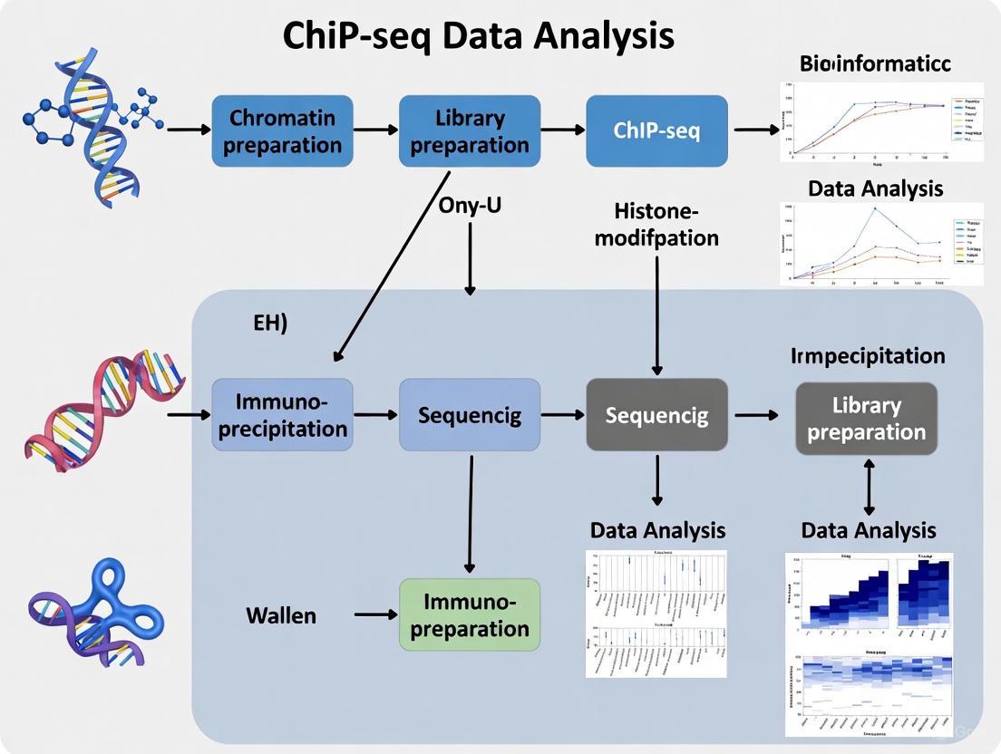
Chromatin Immunoprecipitation followed by sequencing (ChIP-seq) is an instrumental method for capturing a genome-wide snapshot of protein-DNA interactions and histone modifications in their native chromatin context. This technique provides critical insights into the epigenetic regulation of gene expression, enabling researchers to identify regulatory elements, map patterns of histone modifications, and decipher chromatin states in health and disease conditions. For researchers focused on histone modifications, ChIP-seq offers a powerful approach to investigate how post-translational modifications to histones—such as methylation, acetylation, phosphorylation, and ubiquitination—influence chromatin dynamics and gene expression landscapes. The ability to study these modifications within a physiological context makes ChIP-seq particularly valuable for drug development professionals seeking to understand epigenetic therapeutic mechanisms.

Core Principles of ChIP-seq

At its core, ChIP-seq combines immunoprecipitation with next-generation sequencing to map binding sites of DNA-associated proteins across the genome. The technique relies on antibodies to selectively enrich for specific chromatin fragments containing the protein or modification of interest. For histone modification studies, this typically involves antibodies that recognize specific histone marks such as H3K9me2 (a repressive mark) or H3K9me1 (an activating mark). The key requirement is that the antibody must be highly specific to the target epitope, as nonspecific antibodies can generate misleading results by pulling down unrelated chromatin regions [11].

The ChIP-seq procedure involves multiple critical stages: crosslinking to stabilize protein-DNA interactions, cell lysis to liberate cellular components, chromatin fragmentation to generate workable DNA pieces, immunoprecipitation to enrich for target-bound chromatin, and finally sequencing library preparation to enable genome-wide analysis. When studying histone modifications, researchers must consider whether to use crosslinked or native ChIP approaches, as some histone-DNA interactions are sufficiently stable to forego crosslinking [11].

The ChIP-seq Workflow: A Step-by-Step Protocol

Step 1: Crosslinking

The ChIP-seq procedure begins with covalent stabilization of protein-DNA complexes using crosslinking reagents. Formaldehyde is the most commonly used crosslinker, ideal for direct protein-DNA interactions due to its zero-length crosslinking properties. For more complex higher-order interactions or challenging chromatin targets, researchers may implement a double-crosslinking approach using formaldehyde in combination with longer crosslinkers such as EGS (ethylene glycol bis(succinimidyl succinate)) or DSG (disuccinimidyl glutarate) [11] [12].

Critical Considerations: Crosslinking time must be carefully optimized—too little time results in inefficient crosslinking, while excessive crosslinking can cause difficulty with chromatin fragmentation and reduce shearing efficiency. The reaction must be promptly quenched to ensure consistent crosslinking duration across samples [11].

Figure 1: Crosslinking strategies for stabilizing protein-DNA complexes. Formaldehyde works for direct interactions, while longer crosslinkers (DSG/EGS) trap larger complexes.

Step 2: Cell Lysis and Chromatin Extraction

Following crosslinking, cell membranes are dissolved using detergent-based lysis solutions to liberate cellular components. For tissue samples, this step requires additional optimization due to the dense and heterogeneous nature of solid tissues. The refined protocol for tissues includes mincing frozen tissues under cold conditions, followed by homogenization using either a semi-automated gentleMACS Dissociator or a manual Dounce tissue grinder [13].

Critical Considerations: Protease and phosphatase inhibitors are essential at this stage to maintain intact protein-DNA complexes. Successful cell lysis can be visualized under a microscope by comparing samples before and after lysis. For difficult-to-lyse cell types, increasing incubation time in lysis buffer, brief sonication, or using a glass Dounce homogenizer may be necessary [13] [11].

Step 3: Chromatin Shearing

The extracted chromatin must be fragmented into smaller, workable pieces typically ranging from 200-700 bp. This can be achieved either mechanically by sonication or enzymatically using micrococcal nuclease (MNase) digestion [11].

Comparison of Chromatin Fragmentation Methods:

Parameter	Sonication	MNase Digestion
Fragment Distribution	Truly randomized fragments	Preferentially cleaves internucleosomal regions
Reproducibility	Requires significant optimization	Highly reproducible once optimized
Equipment Needs	Dedicated sonication equipment	Standard laboratory equipment
Temperature Sensitivity	Must be kept cold to prevent protein denaturation	Less sensitive to temperature fluctuations
Hands-on Time	Extended hands-on time	More amenable to processing multiple samples

Critical Considerations: When using sonication, keep chromatin on ice at all times and avoid pulses longer than 30 seconds to prevent protein denaturation from excessive heat. For MNase digestion, be aware that enzyme activity variability can affect results, and the approach is less random than sonication [11].

Step 4: Immunoprecipitation

This crucial step uses antibodies specific to the target protein or histone modification to selectively enrich for relevant chromatin fragments. The sheared chromatin is incubated with the antibody, followed by precipitation using protein A/G beads. For histone modification studies, antibody specificity is paramount—the antibody should recognize only the specific modification of interest without cross-reactivity to similar epitopes [11].

Critical Considerations: Always include appropriate controls: a "no-antibody control" (mock IP) for each IP, a known enriched region as a positive control, and a non-enriched region as a negative control. For a standard protocol, use approximately 2×10⁶ cells per immunoprecipitation, though recent advancements have enabled ChIP with significantly fewer cells [11].

Step 5: Library Preparation and Sequencing

Following immunoprecipitation, the enriched DNA is purified and prepared for sequencing. Library construction involves end-repair and A-tailing, adapter ligation with platform-specific adaptors, and PCR amplification. The refined protocol incorporates multi-stage quality checkpoints to ensure library integrity [13]. Recent advancements include compatibility with various sequencing platforms, including the Complete Genomics/MGI sequencing platform which uses DNA nanoballs (DNBs) preparation for cost-effective sequencing, particularly beneficial for large cohort studies [13].

Figure 2: Library preparation workflow for next-generation sequencing following chromatin immunoprecipitation.

ChIP-seq Data Analysis Workflow

The computational analysis of ChIP-seq data involves multiple steps from raw data processing to biological interpretation. Automated platforms like H3NGST (Hybrid, High-throughput, and High-resolution NGS Toolkit) have emerged to streamline this process, providing end-to-end solutions that require minimal bioinformatics expertise [14].

Key Steps in ChIP-seq Data Analysis:

• Raw Data Acquisition and Quality Control: Sequencing reads are retrieved (often from public repositories like SRA) and subjected to quality assessment using tools like FastQC to detect adapter contamination and low-quality reads [14].

• Pre-processing: Adapter sequences are removed and low-quality bases trimmed using tools like Trimmomatic [14].

• Sequence Alignment: Processed reads are aligned to a reference genome (e.g., hg38, mm10) using aligners such as BWA-MEM, generating SAM files that are then converted to BAM format [14].

• Peak Calling: This critical step identifies genomic regions with significant enrichment of sequencing reads using algorithms like HOMER or MACS2. For histone modifications, which often form broad domains, specialized peak-calling algorithms are necessary [14].

• Downstream Analysis: Identified peaks are annotated with genomic features, analyzed for motif enrichment, and interpreted in biological contexts through functional enrichment analyses [14].

The Scientist's Toolkit: Essential Research Reagents and Materials

Reagent/Material	Function	Application Notes
Formaldehyde	Primary crosslinker for stabilizing direct protein-DNA interactions	Concentration and incubation time require optimization for different sample types [11]
EGS or DSG	Longer crosslinkers for stabilizing complex protein interactions	Used in combination with formaldehyde for double-crosslinking protocols [11] [12]
Protease Inhibitors	Prevent protein degradation during cell lysis and chromatin preparation	Essential for maintaining intact protein-DNA complexes [13] [11]
Micrococcal Nuclease (MNase)	Enzymatic fragmentation of chromatin	Provides more reproducible fragmentation compared to sonication [11]
Specific Antibodies	Target immunoprecipitation of specific proteins or histone modifications	Specificity is critical; validate for ChIP applications [11]
Protein A/G Beads	Capture antibody-chromatin complexes during immunoprecipitation	Magnetic beads facilitate easier washing and elution [11]
Dounce Homogenizer or gentleMACS Dissociator	Tissue homogenization for chromatin extraction	Essential for processing solid tissues [13]

Quality Control and Troubleshooting

Key Quality Control Metrics in ChIP-seq:

QC Metric	Target Value	Significance
Chromatin Fragment Size	200-700 bp	Optimal size for sequencing library preparation [11]
Post-IP DNA Concentration	>1 ng/μL	Sufficient material for library preparation
Crosslinking Efficiency	Experiment-specific	Balance between sufficient stabilization and efficient shearing
Peak Distribution	Consistent with expected pattern	E.g., promoter-proximal for certain transcription factors
FRIP (Fraction of Reads in Peaks)	>1% (histone marks), >5% (TFs)	Measure of signal-to-noise ratio [14]

Common challenges in ChIP-seq include low signal-to-noise ratio, incomplete chromatin fragmentation, and antibody nonspecificity. The double-crosslinking approach (dxChIP-seq) has been shown to improve data quality and enhance detection of challenging chromatin targets, particularly for factors that don't bind DNA directly [12]. For tissue samples, optimized handling procedures help preserve tissue-specific chromatin features and enhance output data quality [13].

Applications in Histone Modification Research

ChIP-seq provides unparalleled insights into the genome-wide distribution of histone modifications, enabling researchers to:

• Map repressive and activating histone marks across the genome
• Identify enhancer regions marked by specific histone modifications
• Investigate changes in histone modification patterns in response to epigenetic therapeutics
• Correlate histone modification landscapes with gene expression data

The ability to study histone modifications in tissue contexts provides insights into how gene regulation is shaped by tissue organization and highlights regulatory mechanisms that might be concealed in cell line models [13].

Future Perspectives

As ChIP-seq technologies continue to evolve, several emerging trends are shaping their application in histone modification research. International consortia are working to address coverage gaps in transcription factor ChIP-seq data, with similar implications for histone modification studies [15]. Automated analysis platforms are making ChIP-seq more accessible to researchers without specialized bioinformatics expertise [14]. Additionally, adaptations for low-input samples and solid tissues are expanding the physiological relevance of ChIP-seq findings [13].

For drug development professionals, these advancements mean more comprehensive epigenetic profiling capabilities that can illuminate mechanisms of epigenetic therapeutics and identify novel therapeutic targets in chromatin regulation.

Key Advantages of ChIP-seq for Histone Marks Over Array-Based Methods

The dynamic modification of histones plays a fundamental role in transcriptional regulation by altering chromatin packaging and modifying the nucleosome surface [16]. To understand these epigenetic mechanisms, researchers require robust methods for genome-wide profiling of histone modifications. Chromatin Immunoprecipitation followed by sequencing (ChIP-seq) has emerged as the predominant method for this purpose, largely superseding earlier array-based approaches (ChIP-chip) [16] [17]. This application note delineates the key advantages of ChIP-seq for histone mark analysis within the context of a comprehensive ChIP-seq data analysis workflow, providing researchers, scientists, and drug development professionals with critical insights for experimental design.

Comparative Analysis: ChIP-seq vs. Array-Based Methods

The transition from ChIP-chip to ChIP-seq represents a significant technological shift driven by substantial improvements in data quality, resolution, and practicality. The Table 1 summarizes the quantitative and qualitative differences between these methodologies, synthesized from empirical comparisons [17].

Table 1: Comprehensive Comparison of ChIP-chip and ChIP-seq Technologies

Parameter	ChIP-chip	ChIP-seq
Maximum Resolution	Array-specific, generally 30-100 bp	Single nucleotide
Coverage	Limited by sequences on the array; repetitive regions are usually masked out	Limited only by alignability of reads to the genome; increases with read length; many repetitive regions can be covered
Flexibility	Dependent on available products; multiple arrays may be needed for large genomes	Genome-wide assay for any sequenced organism
Platform Noise	Cross-hybridization between probes and nonspecific targets	Some GC bias can be present
Experimental Design	Single- or double-channel, depending on the platform	Single channel
Required ChIP DNA	High (a few micrograms)	Low (10-50 ng)
Dynamic Range	Lower detection limit; saturation at high signal	Not limited
Cost-Effectiveness	Profiling of selected regions; when a large fraction of the genome is enriched	Large genomes; when a small fraction of the genome is enriched
Multiplexing	Not possible	Possible

Critical Advantages for Histone Mark Analysis

For histone modification studies specifically, ChIP-seq offers several decisive advantages:

• Superior Resolution: ChIP-seq provides single-nucleotide resolution, enabling precise mapping of histone mark boundaries and nucleosome positioning [17]. This is particularly valuable for distinguishing closely spaced epigenetic features, such as bivalent promoters marked by both activating (H3K4me3) and repressing (H3K27me3) modifications [18].

• Unrestricted Genome Coverage: Unlike array-based methods constrained by predefined probe sets, ChIP-seq can interrogate any sequenced genome comprehensively, including repetitive regions that are typically masked in microarray designs [17]. This enables discovery of histone modifications in previously unannotated genomic regions.

• Enhanced Dynamic Range and Sensitivity: ChIP-seq exhibits a broader dynamic range without signal saturation at high levels of enrichment [17]. This allows for more accurate quantification of histone modification density, which is crucial for correlating epigenetic states with transcriptional activity.

ChIP-seq Experimental Workflow for Histone Modifications

A robust ChIP-seq protocol is essential for generating high-quality histone modification data. The following detailed methodology synthesizes best practices from established workflows [16] [19] [17].

Figure 1: ChIP-seq Workflow for Histone Modifications. Key stages include sample preparation (yellow), immunoprecipitation (green), and sequencing/analysis (blue), with a critical quality control checkpoint after chromatin fragmentation.

Crosslinking and Chromatin Preparation

For histone modification analysis, crosslink proteins to DNA using formaldehyde (1-3% final concentration) for 8-15 minutes at room temperature [16] [20]. Quench the reaction with 125 mM glycine for 5 minutes. Isolve nuclei using cell lysis buffer (5 mM PIPES pH 8, 85 mM KCl, 1% Igepal) supplemented with protease inhibitors (PMSF, aprotinin, leupeptin) [16].

Chromatin Fragmentation

For histone modifications, fragmentation via micrococcal nuclease (MNase) digestion is preferred as it generates mononucleosome-sized fragments, providing high-resolution data for nucleosome modifications [19]. Alternatively, sonication of cross-linked chromatin in SDS-containing buffers may be necessary for certain histone epitopes buried within the nucleosome core, such as H3K79me [19].

• Critical Optimization: The optimal size range of chromatin fragments for ChIP-seq should be between 150-300 bp, equivalent to mono- and dinucleosome fragments [19]. Verify fragment size distribution using agarose gel electrophoresis or bioanalyzer before proceeding.

Immunoprecipitation

The quality of antibodies is arguably the most critical factor in successful ChIP-seq experiments [19] [17].

• Antibody Selection: Use ChIP-validated antibodies that demonstrate ≥5-fold enrichment in ChIP-PCR assays at positive-control regions compared to negative controls [19]. For key histone modifications, proven antibodies include:

  • H3K4me3: Anti-Tri-Methyl-Histone H3 (Lys4) (C42D8) rabbit monoclonal antibody (CST #9751S)
  • H3K27me3: Anti-Tri-Methyl-Histone H3 (Lys27) (C36B11) rabbit monoclonal antibody (CST #9733S)
  • H3K9me3: Anti-Tri-Methyl-Histone H3 (Lys9) rabbit antibody (CST #9754S) [16]

• Immunoprecipitation Protocol: Incubate fragmented chromatin with antibody-bound Protein G beads (4°C overnight). Follow with stringent washes using IP dilution buffer (50 mM Tris-HCl pH 7.4, 150 mM NaCl, 1% Igepal, 0.25% deoxycholic acid, 1 mM EDTA) [16].

Library Preparation and Sequencing

After reverse crosslinking (65°C for 4 hours) and DNA purification, prepare sequencing libraries using platform-specific protocols. For Illumina platforms, this includes end-repair, A-tailing, adapter ligation, and PCR amplification [16] [17]. Recent advancements like HT-ChIPmentation have dramatically reduced library preparation time by combining tagmentation with high-temperature reverse crosslinking, enabling single-day data generation [21].

• Sequencing Depth: The ENCODE consortium recommends 20-40 million reads per histone modification ChIP-seq sample for mammalian genomes, with higher depth required for broader marks like H3K27me3 [17].

The Scientist's Toolkit: Essential Research Reagents

Table 2: Key Research Reagent Solutions for Histone Modification ChIP-seq

Reagent Category	Specific Examples	Function & Importance
Validated Antibodies	Anti-H3K4me3 (CST #9751S), Anti-H3K27me3 (CST #9733S), Anti-H3K9me3 (CST #9754S) [16]	Specific recognition of target histone modifications; most critical factor for success
Crosslinking Reagents	Formaldehyde (37%), Glycine [16]	Preserve protein-DNA interactions in their native state
Chromatin Fragmentation Enzymes	Micrococcal Nuclease (MNase) [19]	Generates mononucleosome-sized fragments for high-resolution mapping
Protease Inhibitors	PMSF, Aprotinin, Leupeptin [16]	Prevent degradation of histone proteins and modifications during processing
ChIP-Grade Beads	Protein G-coupled Dynabeads [21]	Efficient capture of antibody-chromatin complexes
Library Preparation	TruSeq DNA Sample Prep Kit (Illumina) [22]	Preparation of sequencing-compatible libraries from immunoprecipitated DNA

Advanced Applications and Recent Methodological Developments

The fundamental advantages of ChIP-seq have enabled increasingly sophisticated epigenetic analyses. Recent innovations further enhance its utility for histone mark profiling:

Scalable and Sensitive Methodologies

HT-ChIPmentation represents a significant advancement, eliminating DNA purification prior to library amplification and reducing reverse-crosslinking time from hours to minutes [21]. This protocol is compatible with very low cell numbers (few thousand cells), making it ideal for rare cell populations or clinical samples with limited material [21].

Integration with Three-Dimensional Genome Architecture

Micro-C-ChIP combines Micro-C with chromatin immunoprecipitation to map 3D genome organization at nucleosome resolution for defined histone modifications [23]. This approach enables researchers to study histone-mark-specific chromatin folding, such as H3K4me3-mediated promoter-promoter interactions, at a fraction of the sequencing cost required for whole-genome methods [23].

Quantitative Comparison Frameworks

Methods like MAnorm have been developed specifically for quantitative comparison of ChIP-seq data sets, allowing researchers to precisely measure differences in histone modification levels across cellular conditions [24]. This normalization approach uses common peaks as a reference to build a rescaling model, effectively addressing technical variations between samples [24].

ChIP-seq provides undeniable advantages over array-based methods for histone modification analysis, including superior resolution, comprehensive coverage, broader dynamic range, and reduced input requirements. These technical benefits have established ChIP-seq as the gold standard for epigenomic profiling, enabling discoveries about the fundamental role of histone modifications in gene regulation, development, and disease. When implemented with careful attention to antibody validation, appropriate controls, and optimized bioinformatic analysis, ChIP-seq delivers unparalleled insights into the epigenetic mechanisms governing cellular function.

In the analysis of chromatin immunoprecipitation followed by sequencing (ChIP-seq) data, the genomic distribution pattern of histone modifications—specifically whether they form sharp, narrow peaks or broad, extended domains—provides critical information that extends beyond mere presence or absence. These patterns are not merely structural artifacts but represent fundamental functional states of the genome with distinct biological implications [25] [26]. While most histone modifications exhibit sharp peaks localized precisely at specific genomic elements like transcription start sites (TSS), a subset of marks, particularly H3K4me3, can form broad domains spanning several kilobases across gene bodies [26]. This application note examines three crucial histone modifications—H3K4me3, H3K27ac, and H3K27me3—within the context of ChIP-seq data analysis workflows, focusing specifically on interpreting their distribution patterns to extract meaningful biological insights for research and drug development.

The recognition that breadth of histone modifications contains biologically significant information represents a paradigm shift in epigenomic analysis. For the active mark H3K4me3, broad domains have been consistently observed across numerous cell types and species, extending up to 60 kilobases from transcription start sites [26]. These broad domains are functionally distinct from their sharp counterparts and require specialized analytical approaches for proper identification and interpretation within ChIP-seq workflows.

Biological Significance and Functional Correlations

H3K4me3: From Sharp Promoter Peaks to Broad Cell Identity Domains

H3K4me3 is one of the most well-characterized histone modifications, traditionally known as a mark of active promoters [27]. In standard ChIP-seq analyses, H3K4me3 typically appears as sharp, narrow peaks (< 1 kb) positioned near transcription start sites, with its intensity generally correlating with transcriptional activity [25]. However, a functionally significant subset of genes in any given cell type displays broad H3K4me3 domains (> 4 kb) that extend downstream from the TSS into the gene body, exhibiting lower signal intensity than sharp peaks but covering substantially more genomic territory [25] [26].

The biological implication of this distribution pattern is profound: genes marked by the broadest H3K4me3 domains (top 5% by breadth) in a particular cell type are consistently enriched for genes essential to that cell's identity and specialized function [26]. In embryonic stem cells, these broad domains mark key pluripotency regulators; in neural progenitor cells, they identify novel regulators of neural development; in contractile cells, they mark genes for specialized cytoskeleton components [26]. This pattern holds across diverse cell types and species, suggesting an evolutionarily conserved mechanism for marking cell identity genes.

Unlike sharp H3K4me3 peaks, broad domains do not correlate with higher expression levels but instead associate with enhanced transcriptional consistency (reduced cell-to-cell variability) [26]. These domains also show increased marks of elongation and more paused polymerase at their promoters, suggesting a unique transcriptional output mechanism focused on precision rather than amplitude [26]. From a therapeutic perspective, reducing expression of genes with broad H3K4me3 domains may increase metastatic potential in cancer cells, highlighting their clinical relevance [25].

H3K27ac: The Active Enhancer Distinction

H3K27ac is a well-established mark of active enhancers and promoters, distinguishing active regulatory elements from their poised counterparts [28] [29]. This modification typically exhibits sharp peak patterns at both proximal and distal regulatory regions, with its presence indicating active engagement of transcriptional coactivators [28].

Functionally, H3K27ac demonstrates an antagonistic relationship with H3K27me3, as both modifications target the same lysine residue [28] [30]. While H3K27ac is considered a gold standard for identifying active enhancers, recent research surprisingly demonstrates that H3K27ac alone may not be functionally determinative for enhancer activity [29]. In mouse embryonic stem cells where H3K27ac was dramatically reduced at enhancers through H3.3K27R mutation, the transcriptome remained largely undisturbed, with maintained chromatin accessibility, H3K4me1 marking, and acetylation at other lysine residues [29].

This finding has significant methodological implications: while H3K27ac remains a valuable indicator of enhancer activity, its presence should be interpreted as part of a broader regulatory context rather than as a sole determinant of transcriptional output in ChIP-seq analyses.

H3K27me3: Repressive Domains with Complex Profiles

H3K27me3 represents the canonical repressive histone mark, deposited by Polycomb Repressive Complex 2 (PRC2) and associated with facultative heterochromatin formation and transcriptional repression [30]. ChIP-seq analyses reveal that H3K27me3 exhibits complex distribution patterns with significant regulatory consequences [31].

Three distinct H3K27me3 enrichment profiles have been identified through systematic ChIP-seq analysis [31]:

• Broad domains spanning entire gene bodies, corresponding to the canonical view of H3K27me3 as inhibitory to transcription
• Focal peaks around transcription start sites, often associated with 'bivalent' genes that also carry H3K4me3 marks
• Promoter peaks surprisingly associated with active transcription in specific contexts

The broad repressive domains of H3K27me3 can spread over hundreds of kilobases, particularly at gene clusters like the Hox genes, creating stable repressive environments [31] [30]. These domains are dynamically remodeled during development and differentiation, with their redistribution preserving cell fate decisions [31].

Table 1: Functional Correlations of Histone Mark Distribution Patterns

Histone Mark	Distribution Pattern	Genomic Location	Functional Correlation
H3K4me3	Sharp, narrow peaks (<1 kb)	Transcription start sites	Active promoters; correlates with transcription levels
	Broad domains (>4 kb)	Gene bodies	Cell identity genes; transcriptional consistency; low variability
H3K27ac	Sharp peaks	Active enhancers and promoters	Distinguishes active from poised regulatory elements
H3K27me3	Broad domains	Gene bodies	Stable transcriptional repression; facultative heterochromatin
	Focal peaks	Transcription start sites	Bivalent promoters (with H3K4me3); poised transcriptional state

Quantitative Analysis and Classification Standards

Defining Sharp vs. Broad: Computational Thresholds

The classification of histone marks as "sharp" versus "broad" requires establishing quantitative thresholds that can be consistently applied across ChIP-seq datasets. For H3K4me3, the field has converged on specific size-based classifications:

• Sharp H3K4me3 domains: Typically < 1-2 kilobases in breadth, concentrated around transcription start sites [25] [26]
• Broad H3K4me3 domains: Typically > 4 kilobases, extending throughout gene bodies, with the most significant functional associations found in the top 5% broadest domains [26]

The breadth of a domain is calculated from ChIP-seq data as the continuous genomic region exhibiting statistically significant enrichment over background, with careful normalization to account for technical variables such as sequencing depth and antibody efficiency [26].

Distribution Patterns Across Genomic Contexts

Different histone modifications exhibit characteristic distribution patterns that provide clues to their functional roles:

Table 2: Characteristic Distribution Patterns of Histone Modifications

Histone Modification	Primary Genomic Context	Typical Breadth	Relationship with Gene Expression
H3K4me3	Promoters, transcription start sites	Sharp: <1-2 kb; Broad: >4 kb	Broad domains mark cell identity genes with consistent expression
H3K27ac	Active enhancers, promoters	Sharp peaks	Indicates active regulatory elements, but not always determinative
H3K27me3	Facultative heterochromatin, repressed genes	Broad domains or focal peaks	Generally repressive, but promoter peaks can coexist with transcription
H3K4me1	Primed and active enhancers	Variable	All enhancers (with H3K27ac distinguishing active ones)
H3K36me3	Gene bodies	Broad domains	Active transcription elongation

Analysis of H3K27me3 patterns requires special consideration, as its functional impact varies significantly based on distribution. Genes with broad H3K27me3 domains across their bodies are consistently repressed, while those with focal promoter peaks may exhibit more complex regulatory patterns, including bivalency with H3K4me3 [31] [30].

Experimental Protocols for ChIP-seq Analysis

Standard ChIP-seq Workflow for Histone Modifications

The following protocol outlines the standard workflow for ChIP-seq analysis of histone modifications, with specific considerations for distinguishing sharp versus broad domains:

Cell Culture and Crosslinking

• Culture cells under appropriate conditions (e.g., mouse embryonic stem cells in DMEM with 15% FCS, LIF, and β-mercaptoethanol) [31]
• Grow cells to ~80% confluence
• Fix cells with 1% buffered formaldehyde for 10 minutes at room temperature [31]
• Quench crosslinking with 125 mM glycine

Chromatin Preparation and Fragmentation

• Prepare chromatin from fixed cells
• Sonicate chromatin to produce fragments from 200-1000 bp, with peak signal between 200-500 bp [31]
• Use approximately 2×10^7 cell equivalents for each immunoprecipitation
• Remove 1.7% of sample for input control [31]

Immunoprecipitation

• Perform immunoprecipitation with validated antibodies:
  • H3K27me3 (07-449, Millipore) [31]
  • H3K4me3 (multiple validated sources)
  • H3K27ac (multiple validated sources)
• Include control rabbit IgG (e.g., ab46540) [31]
• Use protein A/G beads for precipitation
• Wash beads sequentially with low salt, high salt, and LiCl buffers

Library Preparation and Sequencing

• Size-select ChIP-enriched DNA fragments (~200 bp) on agarose gel [31]
• Add sequencing adapters and amplify library using PCR
• Sequence using standard 36 bp or longer single-end protocols on Illumina platforms [31]
• Ensure sufficient sequencing depth (typically 20-40 million reads per sample for mammalian genomes)

Quality Control Considerations

• Antibody Validation: Use antibodies with validated specificity for the intended modification, as cross-reactivity can occur (e.g., some H3K4me3 antibodies may cross-react with H3K4me1 or H3K4me2) [25]
• Input Control: Always include matched input DNA controls for background subtraction
• Replication: Perform biological replicates to ensure consistency (typically n≥2)
• Spike-in Controls: Consider using spike-in controls for normalization when comparing different cell types or conditions

Data Analysis Workflow for Pattern Classification

Preprocessing and Peak Calling

The analytical workflow for distinguishing sharp versus broad domains requires specific computational approaches:

Read Alignment and Processing

• Adapter trimming and quality control (FastQC)
• Alignment to reference genome (Bowtie2, BWA)
• Duplicate removal and fragment size estimation

Peak Calling and Domain Identification

• Use peak callers appropriate for broad domains (e.g., SICER, BroadPeak) in addition to standard peak callers (MACS2) [26]
• For H3K4me3 breadth analysis, specifically employ algorithms that capture extended domains rather than focal peaks
• Normalize signals across samples using robust methods

Classification of Sharp vs. Broad Domains

• Calculate breadth as the continuous enriched region size
• Establish cell-type-specific thresholds based on breadth distribution
• Classify domains: <1-2 kb as sharp, >4 kb as broad, with special attention to top 5% broadest domains [26]

Figure 1: Comprehensive ChIP-seq Workflow for Histone Modification Analysis. The diagram outlines key stages from sample preparation through data interpretation, highlighting quality control checkpoints.

Advanced Analytical Approaches

Multi-mark Integration

• Analyze co-occurrence patterns (e.g., bivalent H3K4me3/H3K27me3 domains)
• Integrate with complementary data (ATAC-seq for accessibility, RNA-seq for expression)
• Employ chromHMM or Segway for chromatin state segmentation [27] [30]

Machine Learning Applications

• Train classifiers to identify cell identity genes based on broad domains [26]
• Use pattern recognition to distinguish functional domain types
• Implement consistency metrics for transcriptional output prediction

Visualization and Interpretation Strategies

Genomic Browser Visualization

Effective visualization is crucial for interpreting sharp versus broad histone modification patterns. The following approaches are recommended:

Multi-track Displays

• Display H3K4me3, H3K27ac, and H3K27me3 in parallel tracks
• Include complementary data (ATAC-seq, RNA-seq, input controls)
• Scale signals appropriately to visualize both sharp and broad features

Domain Classification Visualization

• Use different colors or track heights to distinguish sharp vs. broad domains
• Annotate genes with broad H3K4me3 domains as potential cell identity markers
• Highlight regions with coexisting modifications (bivalent domains)

Quantitative Visualization Approaches

Figure 2: Decision Framework for Classifying Histone Mark Patterns. The workflow illustrates key decision points for categorizing histone modifications as sharp versus broad domains and their distinct functional correlations.

The Scientist's Toolkit: Essential Research Reagents

Table 3: Key Research Reagents for Histone Modification Analysis

Reagent Category	Specific Examples	Function/Application	Considerations
Validated Antibodies	H3K27me3 (Millipore 07-449) [31]	Specific immunoprecipitation of target modification	Validate for ChIP-seq; check for cross-reactivity
	H3K4me3 (multiple vendors)	Marker of active/poised promoters	Some antibodies cross-react with H3K4me1/2 [25]
	H3K27ac (multiple vendors)	Identification of active enhancers	Distinguishes active from poised enhancers
Cell Culture Reagents	Recombinant LIF (Millipore) [31]	Maintenance of pluripotent stem cells	Essential for ES cell culture
	Thrombopoietin [31]	Support of hematopoietic lineages	For specialized cell types
Library Prep Kits	Illumina ChIP-seq kits	Sequencing library preparation	Size selection critical for fragment distribution
Specialized Enzymes	Micrococcal nuclease [27] [30]	Nucleosome positioning studies	Alternative to sonication
	Hyperactive Tn5 transposase [27] [30]	ATAC-seq for chromatin accessibility	Integrative analysis with histone modifications

Troubleshooting and Technical Considerations

Common Analytical Challenges

Domain Boundary Definition

• Challenge: Precisely defining boundaries of broad domains
• Solution: Use multiple algorithms and establish consistency thresholds
• Validation: Compare with orthogonal methods (MNase-seq, ATAC-seq)

Background Subtraction

• Challenge: Differentiating true broad domains from elevated background
• Solution: Implement careful input normalization
• Validation: Include negative control regions

Cell-type Specificity

• Challenge: Distinguishing true biological differences from technical variability
• Solution: Use spike-in controls and robust normalization
• Validation: Analyze replicate consistency and correlation

Advanced Applications

Single-cell Epigenomics

• Emerging technologies enable pattern analysis at single-cell resolution
• Reveals cellular heterogeneity in histone modification patterns
• Requires specialized analytical approaches for sparse data

Dynamic Process Analysis

• Time-course analyses of domain establishment during differentiation
• Integration with transcription factor binding data
• Modeling of epigenetic memory and stability

The distinction between sharp and broad histone modification patterns represents a critical dimension in epigenomic data analysis, extending beyond traditional presence-absence paradigms. For H3K4me3, broad domains specifically mark genes essential for cellular identity and function, exhibiting enhanced transcriptional consistency rather than merely increased expression levels. For H3K27ac and H3K27me3, distribution patterns provide insights into the stability and functional impact of regulatory states. By incorporating pattern classification into standard ChIP-seq workflows and leveraging the experimental and analytical frameworks presented here, researchers can extract deeper biological insights from epigenomic datasets, with particular relevance for understanding cell identity, differentiation, and disease mechanisms in therapeutic development.

The quality of a Chromatin Immunoprecipitation followed by sequencing (ChIP-seq) experiment is fundamentally governed by the specificity of the antibody and the degree of enrichment achieved during immunoprecipitation [32] [19]. For researchers investigating histone modifications, these pre-analytical considerations form the cornerstone of data validity and interpretability. Antibody deficiencies primarily manifest as either poor reactivity against the intended histone modification or cross-reactivity with other chromatin-associated proteins [32]. The ENCODE and modENCODE consortia, through their experience with thousands of ChIP-seq experiments, have developed rigorous working standards and reporting guidelines to provide measures of confidence that the reagent recognizes the antigen of interest with minimal cross-reactivity [32]. This application note outlines critical protocols and considerations to ensure antibody specificity and optimal experimental design prior to computational analysis of histone modification ChIP-seq data.

Antibody Validation Frameworks

Comprehensive Characterization Guidelines

Antibodies used for histone modification ChIP-seq must undergo thorough characterization to establish their specificity and sensitivity. The ENCODE guidelines mandate two complementary tests for antibody characterization [32].

• Primary Characterization: For antibodies against histone modifications, immunoblot analysis serves as the primary characterization method. The guideline specifies that the primary reactive band should contain at least 50% of the signal observed on the blot, ideally corresponding to the expected size of the modified histone [32]. When the main band differs from the expected size by >20% or multiple bands are observed, additional validation through knockdown approaches or mass spectrometry is required.

• Secondary Characterization: Immunofluorescence provides complementary validation by demonstrating expected nuclear staining patterns. Additionally, motif analysis of enriched chromatin fragments can confirm specificity for certain histone modifications, while comparison with multiple antibodies against distinct epitopes or different subunits of protein complexes further verifies specificity [33] [32].

Commercial antibodies designated as ChIP-grade do not always perform adequately for genome-wide studies. As a general rule, antibodies showing ≥5-fold enrichment in ChIP-qPCR assays at several positive-control regions compared to negative control regions typically perform well in ChIP-seq applications [19]. Multiple genomic loci should be tested to account for variation in enrichment across different genomic contexts.

Titration-Based Normalization for Improved Consistency

Recent advances in protocol standardization emphasize the importance of antibody titration for experimental consistency. A 2023 study introduced a quick DNA-based measurement method to quantify chromatin inputs, enabling normalization of antibody amounts to optimal titers in individual ChIP reactions [34].

The methodology involves:

• Direct chromatin quantification: DNA content of chromatin input (DNAchrom) is directly measured using a high-sensitivity double-stranded DNA-specific assay (e.g., Qubit) from a small fraction (0.2%) of total input [34].
• Titer determination: Chromatin input corresponding to 10 μg of DNAchrom is used in ChIP reactions with antibody amounts ranging from 0.05 to 10.0 μg.
• Optimal range identification: The optimal antibody titer is determined based on ChIP yield (DNA amount after ChIP divided by total chromatin input) and fold-enrichment of positive over negative control loci [34].

Table 1: Antibody Titration Optimization Parameters

Parameter	Suboptimal (<0.25 μg/10μg DNAchrom)	Optimal Range (0.25-1 μg/10μg DNAchrom)	Oversaturated (>1 μg/10μg DNAchrom)
ChIP Yield	<0.1%	0.1%-0.5%	>0.5%-5.4%
Fold Enrichment	Variable, often low	5-200-fold (locus dependent)	Dramatically decreased (202 to 18-fold)
Signal-to-Noise	Poor	Optimal	High background

This titration-based normalization significantly improves consistency across samples and experiments, particularly when working with variable chromatin sources such as primary tissues where cellularity and chromatin yield are unpredictable [34].

Experimental Design Considerations

Controls and Replication Strategies

Appropriate control experiments are essential for distinguishing specific enrichment from background noise in histone modification ChIP-seq studies.

• Control Samples: While both non-specific IgGs and chromatin inputs have been used as controls, chromatin inputs are generally preferred as they better account for biases in chromatin fragmentation and variations in sequencing efficiency [19]. Input DNA controls should be sequenced significantly deeper than ChIP samples, particularly for transcription factors and diffuse broad-domain chromatin marks, to ensure sufficient coverage of the genome [35].

• Biological Replicates: To ensure data reliability, duplicate biological experiments should be performed as a minimum standard [19]. Biological replicates account for variability from cell culture conditions, ChIP efficiency, and library construction. When possible, validation with different antibodies against the same histone modification provides additional confirmation of specificity.

• Specificity Controls: For definitive assessment of antibody specificity, knockdown or knockout models where the histone modification is eliminated or reduced provide ideal controls [19]. In these cases, any remaining signal can be attributed to non-specific antibody binding.

Sample Preparation and Sequencing Depth

Effective experimental design requires careful consideration of cellular material and sequencing parameters.

• Cell Number Optimization: ChIP-seq experiments typically require 1-10 million cells, yielding 10-100 ng of ChIP DNA [19]. One million cells often suffices for abundant histone modifications like H3K4me3, while up to ten million cells may be necessary for less abundant modifications. The required sequencing depth depends on genome size and the nature of the histone modification being studied [35].

Table 2: Experimental Design Specifications for Histone Modification ChIP-seq

Experimental Factor	Point-Source Marks (e.g., H3K4me3)	Broad-Source Marks (e.g., H3K36me3)	Mixed-Source Factors
Recommended Cell Number	1-2 million	5-10 million	5-10 million
Sequencing Depth (Mammalian)	20 million reads	Up to 60 million reads	40-60 million reads
Chromatin Fragmentation Size	150-300 bp	150-300 bp	150-300 bp
Fragment Size Selection	Critical for resolution	Important for domain mapping	Essential for both modes
Primary Fragmentation Method	Sonication of cross-linked chromatin	Sonication or MNase digestion	Sonication of cross-linked chromatin

• Sequencing Depth: For mammalian histone modifications, 20 million reads may be adequate for localized marks, while broader chromatin marks require significantly deeper sequencing (up to 60 million reads) [35]. Saturation analysis should be performed to confirm that the chosen sequencing depth adequately captures the biological signal.

Quality Assessment and Troubleshooting

Pre-Sequencing Quality Control

Rigorous quality assessment before sequencing prevents wasted resources on compromised samples.

• Chromatin Fragmentation Quality: The optimal size range of chromatin fragments for ChIP-seq is 150-300 bp, equivalent to mono- and dinucleosome fragments [19]. Fragmentation efficiency should be verified using agarose gel electrophoresis or bioanalyzer profiles after cross-link reversal and DNA purification [16].

• Library Complexity Assessment: Library complexity can be evaluated using the PCR bottleneck coefficient (PBC), defined as the fraction of genomic locations with exactly one unique read versus those covered by at least one unique read [35]. High-quality libraries typically have PBC values >0.8, indicating low redundancy and minimal over-amplification.

• Enrichment Verification: ChIP-qPCR validation of known positive and negative genomic regions should be performed prior to sequencing. A minimum 5-fold enrichment at positive-control regions compared to negative controls generally predicts successful genome-wide experiments [19].

Strand Cross-Correlation Analysis

Strand cross-correlation analysis assesses data quality by measuring the degree of immunoprecipitated fragment clustering [35]. This metric quantifies the cross-correlation between forward and reverse strand read density profiles as a function of shift applied to one strand.

The analysis produces two key metrics:

• Normalized Strand Cross-correlation Coefficient (NSC): Ratio between cross-correlation at fragment length and background cross-correlation. Successful experiments generally have NSC >1.05 [35].
• Relative Strand Cross-correlation Coefficient (RSC): Ratio between cross-correlation at fragment length and cross-correlation at read length. Quality data typically shows RSC >0.8 [35].

Essential Research Reagent Solutions

Table 3: Critical Reagents for Histone Modification ChIP-seq Experiments

Reagent Category	Specific Examples	Function and Application Notes
Validated Antibodies	H3K4me3 (CST #9751S), H3K27ac (Abcam ab4729), H3K27me3 (CST #9733S)	Target-specific immunoprecipitation; require prior validation for ChIP-seq [16] [34]
Chromatin Fragmentation Reagents	Micrococcal Nuclease (MNase), Formaldehyde, Sonication buffers	Chromatin fragmentation; method selection depends on target (MNase for nucleosome mapping, sonication for transcription factors) [19]
Library Preparation Kits	Illumina ChIP-seq Library Prep Kit	End-repair, A-tailing, adapter ligation, and PCR amplification of ChIP DNA [16]
Quality Assessment Tools	Qubit dsDNA HS Assay, Bioanalyzer, FastQC	Quantification and quality control of chromatin input and final libraries [34] [35]
Cell Lysis & IP Buffers	Cell Lysis Buffer, Nuclei Lysis Buffer, IP Dilution Buffer	Cell disruption, nuclear lysis, and immunoprecipitation conditions [16]
Protease Inhibitors	PMSF, Aprotinin, Leupeptin	Prevention of protein degradation during chromatin preparation [16]

Experimental Workflow and Decision Framework

ChIP-seq Antibody Validation Workflow

Histone Modification ChIP-seq Protocol

Robust ChIP-seq data for histone modification studies begins with meticulous attention to pre-analytical factors, particularly antibody specificity and experimental design. The implementation of standardized validation frameworks, titration-based normalization approaches, and comprehensive quality control measures significantly enhances data reliability and reproducibility. By adhering to these detailed protocols for antibody characterization, experimental design, and quality assessment, researchers can generate high-quality epigenomic datasets that accurately reflect the biological reality of histone modification landscapes. These foundational practices ensure that subsequent computational analyses yield meaningful insights into the epigenetic mechanisms governing gene regulation and cellular identity.

A Step-by-Step ChIP-seq Analysis Workflow for Histone Marks

The reliability of Chromatin Immunoprecipitation followed by sequencing (ChIP-seq) data, especially for histone modification studies, hinges on a rigorously optimized experimental design. Within the broader context of a ChIP-seq data analysis workflow for histone modifications research, three interlocking parameters form the foundation of experimental integrity: sequencing depth, biological replication, and appropriate control samples. Insufficient attention to any of these elements can compromise data quality, leading to irreproducible peaks, false discoveries, or an inability to draw meaningful biological conclusions. This document synthesizes guidelines from major consortia like ENCODE and modENCODE and recent methodological advances to provide detailed protocols for designing robust ChIP-seq experiments. The recommendations herein are specifically tailored for researchers and drug development professionals investigating the epigenomic landscape through histone mark profiling, ensuring that generated data is both statistically sound and biologically relevant.

Sequencing Depth Recommendations

Sequencing depth, defined as the number of usable reads uniquely mapped to the reference genome, directly determines the sensitivity and resolution of peak detection [36]. Insufficient depth fails to capture genuine binding sites, particularly for broad histone marks, while excessive depth yields diminishing returns on investment. The optimal depth is not a fixed number but depends on the nature of the histone mark (point-source vs. broad-source), the organism's genome size, and the specific research question.

Guidelines Based on Mark Type and Genome

Deep-sequencing saturation analyses reveal that sufficient depth is reached when detected enrichment regions increase by less than 1% for an additional million sequenced reads [37]. The table below summarizes evidence-based recommendations.

Table 1: Recommended Sequencing Depth for ChIP-seq Experiments

Factor	Organism	Recommended Depth (Million Usable Reads)	Key Considerations
Transcription Factors	Human	10 - 15 [38]	Punctate, narrow peaks; lower depth often sufficient.
Broad Histone Marks (e.g., H3K27me3, H3K9me3)	Human	40 - 50 [37] [39]	Large genomic domains require deeper sequencing for full coverage.
Point-Source Histone Marks (e.g., H3K4me3, H3K27ac)	Human	30 or more [38]	Sharply defined peaks; require less depth than broad marks but more than TFs.
General Marks (Practical Minimum)	Human	40 - 50 [37]	A practical minimum for most marks, though some may require more.
General Marks	D. melanogaster	20 [39]	Smaller genome size reduces the required depth.
Varies with mark	D. melanogaster	< 20 [37]	Sufficient depth is often reached below this point for many marks.

Protocol: Determining Optimal Depth via Saturation Analysis

A key practice is to perform a saturation analysis to empirically determine if a given dataset has reached sufficient depth [37] [36].

• Subsampling Reads: Start with your full, aligned ChIP-seq dataset (e.g., 50 million reads). Use bioinformatic tools (e.g., samtools) to randomly subsample progressively smaller fractions of the total reads (e.g., 10%, 20%, ..., 100%).
• Peak Calling: Perform peak calling on each subsampled dataset using your standard parameters and algorithm.
• Plot Peak Count: Graph the number of peaks called against the number of sequenced reads used for calling.
• Identify Saturation Point: The point where the curve plateaus, and additional reads yield fewer than a 1% increase in detected peaks, is the saturation point. This can be formally defined as the number of reads at which detected enrichment regions increase <1% for an additional million reads [37]. This analysis confirms whether your sequencing depth was adequate or guides future experiments.

Biological Replication Strategies

Biological replicates—independent samples derived from distinct biological units—are non-negotiable for distinguishing consistent biological signals from technical noise and biological variability.

Determining the Number of Replicates

The required number of replicates depends on the goal of the study. The ENCODE consortium guidelines suggest two biological replicates are sufficient for binary site discovery (i.e., identifying if a protein is bound to a specific genomic location) [40] [32]. However, for differential binding analysis—comparing binding affinity or peak size between conditions—more replicates are essential. ChIP-seq data often exhibits higher variance than RNA-seq data, and at least three biological replicates (with four being optimal) per condition are recommended to achieve sufficient statistical power [40] [38]. This allows tools like DESeq2 or Limma to more reliably distinguish true biological changes from background variation.

Protocol: Assessing Replicate Concordance with IDR

The Irreproducible Discovery Rate (IDR) is a robust statistical method used by ENCODE to evaluate reproducibility between replicates [36]. It compares the rank consistency of peaks from two replicates and retains only those that are highly consistent.

• Peak Calling: Call peaks independently on each of your two biological replicates. Use a relaxed threshold (e.g., p-value < 0.05) to generate a large set of peaks, including potential noise.
• Run IDR Analysis: Use the IDR software package to compare the two ranked peak lists from Step 1.
• Generate Conservative Peak Set: IDR outputs a set of high-confidence, reproducible peaks that pass a specified threshold (e.g., IDR < 0.05). This "conservative set" accounts for true biological and technical noise and should be used for downstream analysis.
• Interpret Results: A high IDR consistency score indicates strong reproducibility between your replicates, validating your experimental workflow.

Control Sample Design

Proper controls are critical for accurate peak calling and for attributing observed signals to the specific histone modification of interest.

Types of Controls and Their Applications

Table 2: Essential Control Samples for ChIP-seq Experiments

Control Type	Description	Purpose in Analysis	Protocol Best Practice
Input DNA	Genomic DNA from cross-linked, sonicated chromatin that underwent no immunoprecipitation.	The gold standard control [32]. Accounts for background noise from sequencing biases, open chromatin, and DNA sequence-specific effects. Used by peak callers to calculate significant enrichment.	Always sequence the input control to the same or greater depth as the ChIP sample [37]. Prepare from the same biosample as the ChIP experiment.
IgG Control	Immunoprecipitation with a non-specific antibody (e.g., normal rabbit IgG).	Measures non-specific antibody binding and background caused by the IP process itself.	Use if non-specific binding is a concern. Can be less effective than input DNA for peak calling [32].
Positive Control Antibody	Antibody against a universal DNA-associated protein, such as Histone H3 [41].	Verifies that the entire ChIP protocol (from cross-linking to DNA purification) was successful, independent of your target-specific antibody.	Include in every experiment as a quality control measure. A successful H3 ChIP should yield high signal across the entire genome.
Negative Control Antibody	Non-specific immunoglobulin (IgG) [41].	Distinguishes specific signal from non-specific background. If the target-specific signal is similar to the IgG signal, the antibody may not be working.	Use alongside the positive control to troubleshoot failed experiments.
Spike-in Control	Chromatin or DNA from a distantly related organism (e.g., D. melanogaster chromatin spiked into human samples).	Enables qualitative comparison of binding levels between different conditions, especially when global changes are expected [38].	Normalize your ChIP-seq data based on the read counts aligned to the spike-in genome.

Protocol: Antibody Validation for Histone Modifications

Antibody specificity is the single most critical factor in a ChIP-seq experiment [32]. A poorly characterized antibody can render the entire dataset uninterpretable.

• Primary Characterization (Dot Blot / Peptide Array): Test the antibody's specificity by challenging it with a array of immobilized peptides representing different histone modifications. The antibody should bind strongly only to its intended target modification and show minimal cross-reactivity with similar epitopes.
• Secondary Characterization (Immunoblot): Analyze nuclear or chromatin extracts by western blot. The antibody should produce a single major band at the expected molecular weight for the core histone (e.g., ~15 kDa for Histone H3). The primary reactive band should contain at least 50% of the total signal on the blot [32].
• Reporting: Document all characterization data, including catalog numbers and lot numbers, as antibody performance can vary significantly between lots [38].

Integrated Experimental Workflow

The following diagram synthesizes the key design parameters discussed in this document into a coherent, step-by-step workflow for a robust ChIP-seq experiment.

ChIP-seq Experimental Design Workflow

The Scientist's Toolkit

Table 3: Research Reagent Solutions for ChIP-seq Experiments

Item	Function	Recommendations & Notes
Specific Antibody	Immunoprecipitation of the target histone modification.	Use "ChIP-seq grade" antibodies validated by ENCODE/Epigenome Roadmap if available. Always note catalog and lot numbers [38].
Control Antibodies	Assay quality control.	Positive Control: Anti-Histone H3 [41]. Negative Control: Non-specific species-matched IgG.
Input DNA	Reference control for peak calling.	Essential; prepared from the same cell population as ChIP sample without IP [32].
Spike-in Chromatin	Normalization control for cross-condition comparisons.	Derived from a distant organism (e.g., Drosophila for human samples) [38].
Peak Caller Software	Identification of significantly enriched genomic regions.	MACS2: General purpose, good for sharp peaks [39] [14]. SICER/HOMER: Specialized for broad histone marks [39] [14].
Quality Assessment Tools	Evaluating data quality pre- and post-analysis.	FastQC: Raw read quality [39] [14]. FRiP Score: Fraction of reads in peaks; measures signal-to-noise [36]. IDR: Assesses replicate concordance [36].
Automated Pipelines	Streamlined, end-to-end data analysis.	H3NGST: A fully automated, web-based platform for analysis from raw data to annotation, requiring minimal bioinformatics expertise [14].

Raw Data Acquisition and Quality Control with FastQC

Within a ChIP-seq data analysis workflow for histone modifications research, the initial step of raw data quality control (QC) is paramount for ensuring the validity of all subsequent biological interpretations. Histone modifications, such as H3K27me3 or H3K4me3, typically produce broad enrichment domains across the genome, making data quality a critical factor for accurate peak calling and annotation [42]. FastQC (https://www.bioinformatics.babraham.ac.uk/projects/fastqc/) serves as the first line of defense in this workflow, providing a simple yet powerful way to assess the quality of raw sequencing data coming directly from high-throughput sequencing pipelines [43]. This tool offers a modular set of analyses that provide a quick impression of whether your data has any problems before you invest time and resources in further analysis. By employing FastQC, researchers and drug development professionals can identify common issues such as adapter contamination, low-quality bases, or unexpected sequence composition early in the analysis pipeline, thereby guiding necessary preprocessing steps and ensuring the generation of reliable, publication-quality results [44] [45].

FastQC Installation and Data Requirements

Installation and System Requirements

FastQC is a Java-based application that requires a Java Runtime Environment (JRE) to be installed on the host system. The program, which includes the necessary Picard BAM/SAM libraries, is available for download under the GPL v3 or later license from the Babraham Bioinformatics website [43]. The tool is considered stable and mature, with its most recent update (version 0.12.0) released in January 2023, which introduced enhancements such as improved memory handling, SVG graph generation, and colourblind-friendly colours [43].

Input Data Formats and Acquisition

FastQC accepts raw sequence data in several common formats, making it highly versatile at the start of the ChIP-seq pipeline. The supported formats include:

• FASTQ files (any variant, including those from Illumina, PacBio, and Oxford Nanopore)
• SAM files (Sequence Alignment Map)
• BAM files (Binary Alignment Map) [43]

For ChIP-seq experiments focused on histone modifications, raw data is typically acquired from public repositories like the Sequence Read Archive (SRA) using accession numbers (e.g., BioProject PRJNA, SRA experiment SRX, or GEO sample GSM) [14]. Tools such as prefetch and fasterq-dump are commonly used to retrieve and convert this data into FASTQ format for quality assessment [14]. The ENCODE consortium, which sets standards for histone ChIP-seq experiments, recommends a minimum of 45 million usable fragments per replicate for broad histone marks like H3K27me3 and H3K36me3, and 20 million for narrow marks such as H3K4me3 [42].

Experimental Protocol: Implementing FastQC for ChIP-seq Data

Basic FastQC Operation

The following protocol describes the standard implementation of FastQC within a histone ChIP-seq data analysis workflow.

Materials and Reagents:

• Computational Resources: A computer system with Java Runtime Environment (JRE) installed.
• Input Data: Raw sequencing data in FASTQ, BAM, or SAM format from a histone ChIP-seq experiment.
• Software: FastQC tool (downloadable from https://www.bioinformatics.babraham.ac.uk/projects/fastqc/).

Procedure:

• Data Retrieval: Obtain raw sequencing data from your sequencing facility or public repository. For data from the SRA, use the prefetch utility followed by fasterq-dump for conversion to FASTQ format [14].
• FastQC Execution: Run FastQC on the raw data file using the following command structure:
  Common options include --nogroup to disable the binning of bases for long reads, and --extract to automatically uncompress the output file upon completion [43].
• Report Generation: Upon completion, FastQC generates an HTML-based report in the specified output directory. Open this file in a web browser to review the quality metrics.
• Pre-processing Integration: Based on the FastQC results, proceed with appropriate pre-processing steps such as adapter trimming with tools like Trimmomatic, and then re-run FastQC on the processed data to verify improvement [14] [44].

Advanced Implementation in Automated Pipelines

For high-throughput studies involving multiple histone modification samples, FastQC can be integrated into automated workflows:

In H3NGST Pipeline: The fully automated, web-based H3NGST platform for ChIP-seq analysis incorporates FastQC at two critical points: first on the raw FASTQ files after retrieval from SRA, and again after adapter trimming and quality filtering with Trimmomatic [14]. This dual application provides quality assessment at both the raw and processed stages, ensuring that only high-quality data proceeds to alignment and peak calling.

Batch Processing: FastQC can process multiple files in parallel, a feature particularly useful for ChIP-seq experiments with multiple replicates and input controls [43]. The command structure for batch processing is:

Interpretation of FastQC Results for Histone ChIP-seq

Key Metrics and Their Interpretation

The following table summarizes the core FastQC modules and provides guidance on interpreting their results specifically in the context of histone ChIP-seq data.

Table 1: Comprehensive Guide to FastQC Modules for Histone ChIP-seq Data Interpretation

FastQC Module	What It Measures	Expected Result for Histone ChIP-seq	Potential Issues & Solutions
Per base sequence quality	Distribution of quality scores (Phred) at each base position [45]	Quality scores may start lower in bases 1-5, then rise and gradually decrease toward the 3' end [46].	Sharp quality drops may indicate sequencing issues. Consider trimming low-quality bases [44].
Per sequence quality scores	Average quality per read across its entire length [46]	Tight distribution of reads with high average quality scores.	A significant bump of reads with low average quality may indicate a subpopulation of poor-quality reads requiring removal.
Per base sequence content	Proportion of each nucleotide (A, T, G, C) at every position [45]	Relatively balanced nucleotide distribution across read positions after the first ~10 bases.	Severe bias in initial bases: Common in RNA-seq but not typical in DNA-based ChIP-seq; may indicate library preparation issues [46].
Per sequence GC content	Distribution of GC content across all reads [46]	Distribution approximately normal, centered around the known GC content of the organism.	Unusual peaks or shifts may indicate contamination [45]. A broader distribution is more acceptable for histone ChIP-seq than for whole-genome sequencing.
Sequence duplication levels	Proportion of sequences duplicated at various levels [46]	Low duplication: Expected for diverse ChIP-seq libraries [42]. High duplication may indicate low library complexity or PCR over-amplification.	High duplication: Evaluate library complexity using ENCODE-recommended metrics (NRF, PBC1, PBC2) [42].
Overrepresented sequences	Sequences appearing in >0.1% of total reads [45]	Few to no overrepresented sequences in a high-quality ChIP-seq library.	Presence of adapter sequences indicates need for more aggressive trimming. Common contaminants should be investigated [46].
Adapter content	Proportion of reads containing adapter sequence at each position [46]	Minimal to no adapter content, especially at the 5' end.	Rising adapter content at the 3' end indicates read-through from short inserts, requiring trimming [44].

ChIP-seq Specific Quality Assessment

Beyond standard FastQC metrics, histone ChIP-seq data requires additional quality assessments:

Library Complexity: The ENCODE consortium recommends evaluating library complexity using the Non-Redundant Fraction (NRF) and PCR Bottlenecking Coefficients (PBC1 and PBC2). Preferred values are NRF > 0.9, PBC1 > 0.9, and PBC2 > 10 [42]. These metrics help distinguish between technical duplicates (from PCR amplification) and biological duplicates (genuinely overrepresented sequences).

Strand Cross-Correlation: This ChIP-seq specific metric evaluates the clustering of enriched sequences. For a successful histone ChIP-seq experiment, the cross-correlation should show a clear peak at the predominant fragment length. High-quality experiments typically yield a normalized strand coefficient (NSC) > 1.05 and a relative strand coefficient (RSC) > 0.8 [47] [48].

Integration with Downstream ChIP-seq Analysis

Quality Control Workflow

The following diagram illustrates the position of FastQC within the comprehensive ChIP-seq data analysis workflow for histone modifications.

Diagram 1: ChIP-seq QC and Analysis Workflow

Post-FastQC Quality Assessment

After initial FastQC analysis and preprocessing, histone ChIP-seq data requires additional quality assessments that are specific to the technique:

Fraction of Reads in Peaks (FRiP): This metric calculates the proportion of all mapped reads that fall into called peak regions. A higher FRiP score indicates greater enrichment. The ENCODE consortium recommends minimum FRiP scores of 0.01 for transcription factors and 0.05 for broad histone marks, though successful experiments typically achieve considerably higher values [42] [48].

Peak Concordance and Reproducibility: For replicated experiments, the ENCODE histone pipeline uses either biological replicates or pseudoreplicates to identify stable peaks. Peaks are considered reproducible if they show significant overlap between replicates or pseudoreplicates [42].

Research Reagent Solutions for ChIP-seq QC

Table 2: Essential Research Reagents and Tools for ChIP-seq Quality Control

Resource	Type	Primary Function in ChIP-seq QC	Source/Reference
FastQC	Software Tool	Provides initial quality assessment of raw sequencing data for base quality, GC content, adapter contamination, and overrepresented sequences.	Babraham Institute [43]
Trimmomatic	Software Tool	Removes adapter sequences and trims low-quality bases based on FastQC results, improving overall data quality.	Usadel et al. [14]
BWA-MEM	Software Tool	Aligns sequenced reads to a reference genome, generating BAM files for downstream ChIP-seq specific QC.	Heng Li [14]
HOMER	Software Tool	Performs peak calling and motif analysis; includes utilities for calculating ChIP-seq specific QC metrics.	Heinz et al. [14]
Phantompeakqualtools	Software Tool	Calculates strand cross-correlation metrics (NSC, RSC) specifically for assessing ChIP-seq enrichment quality.	Kundaje et al. [47]
Input Control DNA	Wet-bench Reagent	Matching control sample essential for normalizing ChIP-seq data and accurately calling enriched regions.	ENCODE Guidelines [42]
Histone Modification Antibodies	Wet-bench Reagent	Protein-specific binders for immunoprecipitation; must be thoroughly validated for specificity as per ENCODE standards.	ENCODE Guidelines [42]

FastQC serves as an indispensable first step in the ChIP-seq data analysis workflow for histone modification studies, providing critical insights into data quality that inform all subsequent processing steps. When implemented according to the protocols outlined in this document and interpreted within the context of histone-specific metrics such as those defined by the ENCODE consortium, researchers can reliably identify potential issues early in the analysis pipeline. This proactive approach to quality assessment ensures that downstream biological interpretations—whether for basic research or drug development applications—are grounded in high-quality, reproducible data. The integration of FastQC with ChIP-seq specific QC tools and metrics creates a comprehensive quality framework that maximizes the value of histone modification studies and contributes to robust, publication-ready findings.

Read Mapping to Reference Genomes using BWA-MEM and Bowtie

In chromatin immunoprecipitation followed by sequencing (ChIP-seq) workflows, read mapping is a fundamental computational step that determines where short DNA sequences (reads) originated within a reference genome. This process is essential for identifying protein-DNA interactions and histone modifications across the genome [47] [49]. The accuracy of read alignment directly influences downstream analyses, including peak calling, motif discovery, and the biological interpretation of epigenetic regulation [14]. For histone modification studies, precise mapping is particularly crucial as these marks often exhibit broad enrichment domains that require sensitive detection methods.

The selection of an appropriate alignment tool represents a critical decision point in experimental design. Bowtie2 and BWA (Burrows-Wheeler Aligner) have emerged as two of the most widely used aligners in contemporary ChIP-seq pipelines [50] [51]. Both tools utilize the Burrows-Wheeler Transform (BWT) to efficiently compress and index the reference genome, enabling rapid alignment of millions of short reads while managing computational memory requirements [52] [51]. However, these tools differ in their specific algorithms, performance characteristics, and optimal use cases, necessitating careful consideration of their respective strengths and limitations for histone modification research.

Comparative Analysis of BWA-MEM and Bowtie2

Algorithmic Foundations and Performance Characteristics

Bowtie2 and BWA-MEM employ distinct alignment strategies that impact their performance in ChIP-seq applications. Bowtie2 performs gapped, local alignment using a FM Index-based strategy that excels at aligning reads of 50-1000 base pairs [50] [53]. It supports both end-to-end and local alignment modes, with the latter performing soft-clipping to remove poor quality bases or adapters from untrimmed reads [50]. This flexibility makes Bowtie2 particularly versatile for various sequencing qualities.

BWA-MEM represents a more recent development in the BWA algorithm family, designed to replace earlier implementations (BWA-backtrack and BWA-SW) for most applications [51] [54]. It automatically chooses between local and end-to-end alignments and demonstrates superior performance for reads ranging from 70bp to several megabases [51] [54]. BWA-MEM efficiently handles mismatches and gaps, offering robust performance with paired-end reads, which has established it as a preferred choice for many whole genome sequencing projects [52] [51].

Table 1: Key Characteristics of Bowtie2 and BWA-MEM

Feature	Bowtie2	BWA-MEM
Optimal Read Length	50-1000bp [50]	70bp-1Mbp [51]
Alignment Mode	Local and end-to-end [50]	Automatically selects local/end-to-end [51]
Paired-end Support	Yes [50]	Yes [51]
Typical Use Cases	ChIP-seq, general NGS [50]	Variant calling, whole genome sequencing [51]
Speed	Very fast [52]	Moderate [52]
Accuracy	High [50]	Very high [51]

Performance in ChIP-seq Applications

For ChIP-seq experiments targeting histone modifications, alignment accuracy often takes precedence over speed due to the impact on peak calling sensitivity and specificity. While Bowtie2 is commonly used in ChIP-seq pipelines [50], BWA may provide advantages in certain scenarios. Comparative evaluations have revealed that BWA typically achieves higher mapping rates (approximately 2% greater than Bowtie2) with a corresponding increase in uniquely mapped reads [50]. This enhanced sensitivity can translate to a significantly larger number of peaks being called (up to 30% increase in some comparisons) [50].

However, this increased sensitivity requires careful validation, as it may potentially introduce false positives without appropriate quality control measures [50]. The optimal choice depends on specific experimental factors, including read length, sequencing depth, and the expected characteristics of histone modification patterns. For projects requiring maximal sensitivity to detect broad histone marks, BWA-MEM may be preferable, while Bowtie2 offers excellent performance for more focused binding patterns with faster processing times.

Experimental Protocols

Read Mapping with Bowtie2

The following protocol details the standard procedure for aligning ChIP-seq reads using Bowtie2:

Step 1: Tool Installation and Activation

Step 2: Alignment Execution

Critical Parameters:

• -p: Number of processor cores to use
• --local: Enables local alignment with soft-clipping
• -x: Path to genome indices
• -1/-2: Paired-end read files
• -S: Output SAM file
• --met-file: Alignment metrics output [50]

Step 3: Post-Alignment Processing Convert SAM to BAM format and sort by genomic coordinates:

The sorted BAM file is now ready for quality assessment and downstream analysis [50].

Read Mapping with BWA-MEM

Step 1: Genome Indexing

Step 2: Read Alignment

Critical Parameters:

• -M: Marks shorter split hits as secondary for Picard compatibility
• -t: Number of threads
• Redirecting stderr (2>) captures processing metrics [51]

Step 3: Alignment Cleanup and Duplicate Marking

Duplicate marking is particularly important for variant calling as PCR duplicates can bias variant detection [51].

Workflow Integration and Visualization

The alignment process represents a critical component within the comprehensive ChIP-seq analysis workflow. The following diagram illustrates the position of read mapping within the broader experimental context and the decision process for selecting between alignment tools:

Alignment Tool Selection Logic

The choice between BWA-MEM and Bowtie2 depends on multiple experimental factors. The following decision tree provides guidance for selecting the optimal aligner based on project requirements:

Table 2: Key Research Reagent Solutions for ChIP-seq Read Mapping

Resource Category	Specific Tool/Reagent	Function in Workflow	Implementation Notes
Alignment Algorithms	Bowtie2 [50]	Maps sequencing reads to reference genome	Optimal for standard ChIP-seq; fast processing
	BWA-MEM [51]	Alternative mapping algorithm	Higher sensitivity for certain applications
Quality Control	FastQC [14]	Assesses read quality before/after trimming	Identifies adapter contamination, poor quality bases
	Trimmomatic [14]	Removes adapters, trims low-quality bases	Improves mapping rates and accuracy
Post-Alignment Processing	SAMtools [14] [51]	Converts, sorts, indexes alignment files	Essential for BAM file manipulation
	Picard Tools [51]	Marks PCR duplicates, validates file formats	Reduces artifacts in variant calling
Reference Genomes	hg38, mm10, etc. [14]	Species-specific reference sequences	Must match organism studied
Computational Infrastructure	High-performance computing cluster	Handles memory-intensive alignment tasks	BWA-MEM requires ~30GB RAM for human genome [52]

Troubleshooting and Quality Assessment

Addressing Common Alignment Issues

Researchers may encounter several challenges during read mapping that impact downstream analysis:

Low Mapping Efficiency When a high percentage of reads fail to align (e.g., >90% aligned concordantly 0 times), potential causes include:

• Incorrect library preparation metadata (e.g., treating single-end data as paired-end) [55]
• Reference genome mismatch or poor quality indexing
• Severe adapter contamination not addressed by trimming
• Poor sequence quality or excessive read length degradation

Validation Approach:

• Verify library structure by examining read identifiers in FASTQ files (true paired-end reads have matching identifiers with /1 and /2 or /3 suffixes) [55]
• Re-run quality control with FastQC to identify adapter content or quality issues
• Confirm reference genome build matches experimental organism

Duplicate Reads High duplicate levels (>50%) may indicate:

• PCR amplification artifacts during library preparation
• Insufficient sequencing depth for the genome size
• Genomic DNA contamination [56]

Mitigation Strategies:

• Use Picard's MarkDuplicates to identify and optionally remove duplicates [51]
• Increase sequencing depth if duplicates result from low input material
• Verify library preparation protocols and input DNA quality

Quality Metrics for Alignment Files

After successful alignment, several key metrics determine data quality:

Strand Cross-Correlation For ChIP-seq specific quality assessment, strand cross-correlation analysis evaluates the periodicity of forward and reverse strand tags around binding sites [47]. Key metrics include:

• Normalized Strand Cross-correlation Coefficient (NSC): Values >1.05 indicate successful enrichment
• Relative Strand Cross-correlation (RSC): Values >1.0 suggest good quality, <1.0 indicates poor enrichment [47]

Mapping Statistics

• Uniquely mapped reads: Ideally >70-80% for high-quality data [56]
• Multi-mapped reads: Should be minimized as they can increase false positives [50]
• PCR duplicates: Track percentage marked by Picard tools

The selection between BWA-MEM and Bowtie2 for ChIP-seq read mapping represents a critical methodological decision that influences all subsequent analyses in histone modification research. While both tools provide excellent performance, their relative strengths suit different experimental contexts. Bowtie2 offers exceptional speed and efficiency for standard ChIP-seq applications with typical read lengths (50-1000bp), making it ideal for most histone modification studies. BWA-MEM demonstrates superior sensitivity and accuracy for longer reads (>100bp) and applications requiring maximal mapping rates, though with increased computational requirements.

Successful implementation requires careful attention to quality control throughout the alignment process, including pre-alignment quality assessment, appropriate parameter selection, and post-alignment quality metrics. By following the detailed protocols outlined in this document and utilizing the provided troubleshooting guide, researchers can optimize their read mapping workflow to generate robust, reproducible results for histone modification studies. The integration of these alignment tools within a comprehensive ChIP-seq pipeline enables the precise identification of epigenetic regulatory elements that underlie fundamental biological processes and disease mechanisms.

Within the comprehensive workflow of ChIP-seq data analysis for histone modifications research, peak calling serves as the critical computational step that transforms aligned sequence reads into biologically interpretable regions of protein-DNA interaction. The accuracy of this step directly influences all downstream analyses, from motif discovery to the understanding of epigenetic regulatory mechanisms. Histone modifications manifest in fundamentally different patterns across the genome: sharp marks, such as H3K4me3 and H3K27ac, define precise promoter and enhancer elements, typically spanning a few hundred to a few thousand base pairs, while broad marks, including H3K27me3 and H3K36me3, can spread across extensive genomic domains spanning tens to hundreds of kilobases [57]. These distinct patterns necessitate specialized computational approaches for optimal detection. The selection of an appropriate peak calling algorithm must be guided by the biological characteristics of the histone mark under investigation, as suboptimal tool usage can significantly impact the interpretation of ChIP-seq datasets [57]. This protocol examines three widely adopted tools—MACS2, SICER2, and HOMER—providing performance evaluations, detailed methodologies, and integration strategies tailored for histone modifications research.

Algorithm Performance and Selection Guidelines

Performance Evaluation Across Histone Mark Types

The performance of peak calling algorithms is highly dependent on both the spatial characteristics of the histone mark and the biological regulation scenario. Comprehensive assessments using standardized reference datasets created through in silico simulation and genuine ChIP-seq data subsampling have revealed that tool performance varies significantly based on peak architecture [57]. Transcription factors (TFs) and sharp histone marks like H3K27ac typically occupy defined regions, while broad marks such as H3K36me3 spread over large genomic domains, requiring different analytical approaches.

Table 1: Performance Characteristics of Peak Calling Algorithms

Tool	Primary Design	Optimal Mark Type	Strengths	Limitations
MACS2	Model-based analysis [58]	Sharp marks (H3K4me3, H3K27ac) [59]	High precision-recall for defined peaks; robust normalization [57]	Less effective for diffuse broad domains [57]
SICER2	Spatial clustering approach [60]	Broad marks (H3K27me3, H3K36me3) [57]	Identifies extended enriched domains; handles low signal-to-noise [60]	Suboptimal for narrow, sharp peaks [57]
HOMER	Combinatorial analysis [61]	Both sharp and broad marks	Integrated peak calling and motif discovery [62]	Performance varies significantly by mark type [57]

Evaluation metrics based on the area under the precision-recall curve (AUPRC) demonstrate that while tools like MACS2, MEDIPS, and PePr show high median performance across scenarios, specific parameter optimizations can yield superior results for particular applications [57]. For instance, in systematic evaluations of intracellular G-quadruplex sequencing data—which presents narrow peak patterns—MACS2 and PeakRanger demonstrated superior performance with maximum harmonic mean scores ranging from 0.67 to 0.84, significantly outperforming other algorithms [59].

Selection Guidelines for Different Biological Scenarios

The choice of peak caller should be guided by the experimental design and the specific histone mark under investigation. Researchers should consider two primary biological scenarios when selecting parameters and tools:

• Balanced Regulation Scenarios (50:50 ratio of increasing to decreasing signals): This scenario represents comparisons of developmental or physiological states where some genomic regions show increased binding while others show decreased binding. In such cases, tools that assume most genomic regions do not differ between states (e.g., those adapted from RNA-seq analysis) may perform adequately [57].

• Global Regulation Changes (100:0 ratio): This scenario occurs with global knockdown, knockout, or pharmacological inhibition of the target protein, resulting in widespread loss of histone modifications. In these cases, normalization methods that assume most peaks remain unchanged can produce biased results, requiring specialized tools that accommodate global changes [57].

For broad histone marks, the SICER2 algorithm specifically addresses the challenge of diffuse enrichment patterns through its spatial clustering approach, which identifies statistically significant clusters of adjacent enriched windows rather than individual peaks [60]. Meanwhile, MACS2 with the --broad parameter provides an alternative approach for wider enrichment domains, though benchmarking studies suggest SICER2 may be more specifically optimized for extremely broad marks like γH2Ax [63].

Experimental Protocols and Implementation

MACS2 Implementation for Sharp Histone Marks

MACS2 (Model-based Analysis of ChIP-Seq 2) employs a Poisson distribution or negative binomial distribution to model background read distribution and identify statistically enriched regions [58]. The following protocol is optimized for sharp histone marks such as H3K4me3 and H3K27ac:

Standard Protocol for Sharp Marks:

Key Parameters for Sharp Marks:

• -t: Treatment sample (BAM format)
• -c: Control/input sample (BAM format)
• -f BAM: Input file format
• -g hs: Effective genome size (human: 2.7e9)
• -n: Output file prefix
• -B: Generate bedGraph files for visualization
• -q 0.01: FDR cutoff of 1% for peak detection

For histone marks with broader characteristics, MACS2 offers a broad peak calling mode:

The --broad parameter activates the broad peak calling algorithm, while --broad-cutoff sets the significance threshold (FDR of 10% in this example) [64].

MACS2 generates several output files including NAME_peaks.narrowPeak (containing peak locations and statistics), NAME_summits.bed (precise summit positions for motif analysis), and NAME_model.r (an R script for visualizing the peak model) [58].

SICER2 Implementation for Broad Histone Marks

SICER2 (Spatial Clustering for Identification of ChIP-Enriched Regions) employs a clustering approach specifically designed to identify broad domains of histone modifications by accounting for spatial dependence between adjacent genomic regions [60]. The algorithm identifies significant islands of enriched windows, making it particularly suitable for diffuse marks like H3K27me3.

Standard Protocol for Broad Marks:

Key Parameters for Broad Marks:

• -t: Treatment sample (BAM format)
• -c: Control sample (BAM format)
• -s hg38: Reference genome
• -w 200: Window size (bp) - may be increased to 1000-2000 for very broad marks
• -egf 0.74: Effective genome fraction
• -fdr 0.01: False discovery rate cutoff
• -g 600: Gap size (bp) - maximum gap between significant windows to be merged

For extremely broad marks such as γH2Ax, increasing the window size to 1-2 kb may improve performance, as the default 200 bp window may be suboptimal for detecting extensive enriched domains [63]. The recognicer command provides an alternative algorithm that uses a coarse-graining approach to identify broad domains on multiple scales [60].

SICER2's differential peak calling module (sicer_df) enables comparative analysis between conditions, using the same core parameters with the addition of a false discovery rate cutoff for differential peaks (-fdr_df) [60].

HOMER Implementation for Integrated Peak and Motif Analysis

HOMER (Hypergeometric Optimization of Motif EnRichment) provides an integrated suite for peak calling, annotation, and motif discovery, utilizing a combinatorial approach that supports both sharp and broad mark analysis [62].

Peak Calling Protocol:

Motif Discovery Protocol:

Key Parameters for Histone Modifications:

• -style histone: Optimizes parameters for histone mark analysis
• -o auto: Automatically determines output format
• -size 200: Region size for motif analysis (adjust based on mark)
• -mask: Repeat masking for improved motif discovery

HOMER requires initial data preprocessing to create "tag directories" from BAM files:

For motif analysis, the findMotifsGenome.pl script compares target sequences against background sequences, automatically performing GC-content normalization and oligonucleotide frequency optimization to account for technical and biological biases [62]. The -len parameter allows simultaneous search for multiple motif lengths (e.g., -len 8,10,12), which is particularly valuable for de novo motif discovery in histone mark datasets.

Visualization of Analytical Workflows

Peak Calling Decision Pathway

The following workflow illustrates the systematic selection and application of peak calling algorithms based on experimental objectives and histone mark characteristics:

Comprehensive ChIP-seq Analysis Workflow

The complete analytical pipeline for histone modification studies extends from raw data processing through functional interpretation, with peak calling serving as the central step:

Table 2: Essential Research Reagents and Computational Tools

Category	Item	Specification/Version	Application Purpose
Experimental Reagents	BG4 antibody	N/A	Specific recognition of G4 structures in chromatin [59]
	H3K27me3 antibody	Cell Signaling Technology, 9733s	Immunoprecipitation of H3K27me3 histone marks [65]
	H3K4me3 antibody	Merck, 07-473	Immunoprecipitation of H3K4me3 histone marks [65]
	CTCF antibody	Abcam, ab70303	Immunoprecipitation of CTCF transcription factor [65]
	Hyperactive CUT&Tag Assay Kit	Vazyme Biotech, TD904	Library preparation for CUT&Tag experiments [65]
Software Tools	MACS2	Version 2.x	Primary peak calling for sharp histone marks [58]
	SICER2	Python 3.x version	Spatial clustering for broad histone marks [60]
	HOMER	v4.11+	Motif discovery and integrated peak analysis [62]
	BedTools	v2.30.0+	Genome arithmetic and interval operations [64]
	SAMtools	v1.15+	Processing aligned sequencing files [64]
Reference Data	Genome sequence	hg38, mm10	Species-specific reference genome
	Effective genome size	hs: 2.7e9, mm: 2.1e9	Parameter for peak calling normalization [58]

Discussion: Integration with Emerging Technologies and Method Selection

As chromatin profiling technologies evolve, peak calling algorithms must adapt to new experimental paradigms. Emerging techniques such as CUT&Tag and CUT&RUN offer advantages including reduced background noise and lower input requirements compared to traditional ChIP-seq [65]. These methods produce distinct read distributions that may benefit from optimized peak calling parameters. For example, CUT&Tag datasets often exhibit higher signal-to-noise ratios, potentially enabling more sensitive detection of histone modifications with standard algorithms like MACS2 [65].

The selection of an appropriate peak calling strategy should be guided by the specific histone mark under investigation, the experimental methodology, and the biological question. Benchmarking studies consistently demonstrate that performance varies significantly across tools and parameter settings [57]. For sharp marks, MACS2 frequently achieves superior precision-recall balance, while for broad domains, SICER2's spatial clustering approach provides enhanced sensitivity for detecting extended enriched regions [57] [60]. HOMER offers the advantage of integrated motif discovery, which can directly link histone modification patterns to potential transcription factor binding events [62].

Future directions in peak calling algorithm development will likely focus on improved normalization for complex biological scenarios, enhanced efficiency for single-cell epigenomics data, and more sophisticated integration of multi-omics datasets. As these tools evolve, systematic benchmarking against standardized reference datasets will remain essential for guiding algorithm selection in histone modification research [57].

Genomic Annotation of Peaks and Functional Interpretation

In the context of a comprehensive ChIP-seq data analysis workflow for histone modifications research, genomic peak annotation serves as the critical bridge between identified regions of significant enrichment and their biological interpretation. Chromatin immunoprecipitation followed by sequencing (ChIP-seq) has become an indispensable method for mapping histone modifications across the genome, revealing the epigenetic landscape that influences gene accessibility, cell identity, and disease mechanisms [14] [9]. The process of peak annotation systematically assigns biological meaning to these enriched regions by determining their genomic context relative to known features, thereby transforming coordinate-based results into functionally testable hypotheses.

The fundamental challenge that peak annotation addresses is the non-random distribution of histone modifications throughout the genome. These epigenetic marks exhibit distinct spatial relationships with functional elements: some histone modifications cluster prominently at transcription start sites, while others span broad regulatory domains or gene bodies [49] [9]. Proper annotation allows researchers to move beyond simple lists of genomic coordinates toward understanding how histone modifications organize the regulatory architecture of the genome. This process is particularly crucial for histone modification studies, where the broad nature of many chromatin marks requires specialized analytical approaches compared to transcription factor binding sites [14].

Key Concepts and Categorical Frameworks

Genomic Feature Classification System

Peak annotation employs a hierarchical classification system to categorize histone modification enrichment relative to genomic features. The standard framework assigns each peak to one primary category based on its position relative to gene structures, with promoter-proximal regions receiving highest priority due to their established regulatory significance [66]. This systematic classification enables researchers to quickly assess the functional distribution of their histone modification data and generate biologically relevant hypotheses about regulatory mechanisms.

• Promoter-associated Peaks: Peaks located within 2 kilobases upstream of a transcription start site (TSS) are annotated as promoter peaks, reflecting their potential direct involvement in transcription initiation regulation [66]. Histone modifications enriched in these regions, such as H3K4me3, often mark actively transcribed genes and contribute to accessible chromatin configurations.
• Intragenic Peaks: This category encompasses peaks falling within gene bodies but outside promoter regions, further subdivided into:
  • Intronic Peaks: Located within intronic regions, which may indicate enhancer elements or other regulatory sequences embedded within genes.
  • Exonic Peaks: Found within exonic regions, potentially influencing transcript processing or stability.
• Intergenic Peaks: Peaks located in genomic regions distant from annotated genes, which may represent distal regulatory elements such as enhancers, silencers, or insulator elements [66]. These are typically assigned to the gene whose TSS is closest, enabling linkage of distal regulatory elements with potential target genes.

Annotation Prioritization Logic

The annotation process follows a specific decision hierarchy to ensure consistent and biologically meaningful classification. When a peak overlaps multiple genomic features, the system assigns it to the highest-priority category according to established protocols [66]. This prioritization prevents double-counting and ensures that the most functionally relevant assignment takes precedence, with promoter regions typically receiving highest priority, followed by intragenic features, and finally intergenic regions. This structured approach is particularly valuable for histone modifications that can span large genomic domains and potentially overlap multiple feature types simultaneously.

Experimental Protocols and Methodologies

Programmatic Annotation Using ChIPseeker

For researchers with bioinformatics capabilities, the ChIPseeker package in R provides a powerful and flexible environment for comprehensive peak annotation. The following protocol outlines a standard workflow for annotating histone modification peaks:

Step 1: Environment Setup and Package Loading Initialize the R environment and load required libraries. The ChIPseeker package extends its functionality through integration with other Bioconductor tools for genomic analysis.

Step 2: Annotation Database Preparation Load appropriate transcript database matching the reference genome used for alignment. Consistent genome builds between alignment and annotation are critical for accuracy.

Step 3: Peak Data Import and Processing Import peak files (typically in BED or narrowPeak format) and convert to GRanges object for downstream analysis.

Step 4: Genomic Annotation Execution Perform the actual annotation process, specifying the TSS region parameter to define promoter proximity.

Step 5: Visualization and Result Export Generate visual summaries of annotation results and export annotated peak tables.

Automated Web-Based Annotation with H3NGST

For researchers preferring a code-free environment, the H3NGST platform provides a fully automated, web-based solution for end-to-end ChIP-seq analysis, including comprehensive peak annotation [14]. This approach significantly reduces technical barriers while maintaining analytical rigor.

Step 1: Data Input and Parameter Configuration

• Navigate to the H3NGST web interface (https://ngschiphhh.duckdns.org)
• Input BioProject, SRA, GEO, or other public accession numbers
• Select appropriate reference genome (e.g., hg38, mm10)
• Choose "histone modification" as experiment type for broad peak detection
• Set promoter region definition (default: -2000 to +2000 from TSS)
• Specify false discovery rate threshold (typically 0.05 for histone marks)

Step 2: Pipeline Execution and Monitoring

• Submit analysis job using assigned nickname for result tracking
• System automatically retrieves raw data, performs quality control, adapter trimming, and alignment
• Peak calling is performed with HOMER, optimized for broad histone modification profiles
• Automated annotation executes using integrated gene models

Step 3: Result Retrieval and Interpretation

• Download complete annotation results including:
  • Annotated peak tables with genomic feature assignments
  • Summary statistics of peak distribution across feature types
  • Motif enrichment analysis relative to annotated regions
  • Quality control metrics specific to histone modification experiments

Functional Enrichment Analysis Protocol

Following genomic annotation, functional interpretation identifies biological processes, pathways, and molecular functions associated with annotated peaks.

Step 1: Gene List Preparation Extract genes associated with annotated peaks based on genomic proximity.

Step 2: Functional Enrichment Execution Perform Gene Ontology and pathway enrichment analysis using clusterProfiler.

Step 3: Result Visualization and Interpretation Generate publication-quality visualizations of enrichment results.

Data Presentation and Quantitative Analysis

Typical Peak Distribution Across Genomic Features

Table 1: Representative Distribution of H3K27ac Peaks Across Genomic Regions in Mammalian Cells

Genomic Feature	Percentage of Peaks	Biological Significance
Promoter (≤2 kb from TSS)	25-35%	Marks active enhancers and transcriptional start sites
Intronic	30-40%	Potential enhancer regions, cell-type specific regulatory elements
Exonic	5-10%	Potential impact on transcript processing and stability
Intergenic	20-30%	Distal enhancers, insulators, other regulatory elements
3' UTR	3-5%	Potential role in transcription termination and RNA processing
5' UTR	2-4%	Potential regulation of translation initiation

Data compiled from ENCODE guidelines and experimental observations [67] [66].

Quality Control Metrics for Histone Modification Peak Annotation

Table 2: Essential QC Metrics for Robust Histone Modification Peak Annotation

QC Metric	Target Value	Interpretation Guidelines
Fraction of Reads in Peaks (FRiP)	>1% for broad marks >5% for sharp marks	Measures enrichment efficiency; varies by histone mark
Non-Redundant Fraction (NRF)	>0.9	Indicates library complexity; lower values suggest excessive duplication
Strand Cross-Correlation (NSC)	>1.05	Measures signal-to-noise ratio; higher values indicate stronger enrichment
Strand Cross-Correlation (RSC)	>0.8	Normalized strand correlation; values >1 indicate high-quality ChIP
Peak Reproducibility (IDR)	<0.05 for replicates	Measures consistency between biological replicates
Annotation Consistency	Match established distributions	Significant deviations may indicate technical artifacts

Quality metrics based on ENCODE consortium guidelines and recent implementations [67] [48].

Workflow Visualization

Figure 1: Peak Annotation and Interpretation Workflow. This diagram illustrates the sequential process for annotating ChIP-seq peaks, from initial quality assessment through functional interpretation. The workflow emphasizes the hierarchical prioritization system for genomic feature assignment.

The Scientist's Toolkit

Essential Research Reagent Solutions

Table 3: Key Research Tools and Resources for Peak Annotation

Tool/Resource	Type	Primary Function	Implementation Considerations
ChIPseeker	R/Bioconductor Package	Genomic peak annotation and visualization	Requires R programming knowledge; highly customizable
HOMER	Command-line Suite	Peak calling, annotation, and motif discovery	Comprehensive workflow; steep learning curve
H3NGST	Web Platform	Fully automated annotation pipeline	No installation required; limited customization
ENSEMBL Biomart	Database	Gene model annotations	Essential for current gene annotations
UCSC Known Genes	Database	Conservative gene models	Stable, well-annotated gene set
GENCODE	Database	Comprehensive transcript annotation	Most detailed human and mouse annotations
clusterProfiler	R Package	Functional enrichment analysis	Integrates with ChIPseeker workflow
org.Mm.eg.db	Database	Mouse organism database	Essential for functional annotation in mouse
org.Hs.eg.db	Database	Human organism database	Essential for functional annotation in human

Toolkit compiled from referenced protocols and platforms [68] [14] [66].

Genomic peak annotation represents an indispensable component in the ChIP-seq analysis workflow for histone modification research, transforming coordinate-based enrichment data into biologically meaningful insights. Through systematic categorization of peaks relative to genomic features, followed by functional enrichment analysis, researchers can decipher the complex regulatory code embedded in chromatin landscapes. The protocols and frameworks presented here provide both computational and accessible web-based approaches suitable for diverse research environments and expertise levels. As histone modification studies continue to illuminate mechanisms of gene regulation in development and disease, robust peak annotation practices will remain fundamental to extracting biologically valid conclusions from epigenomic datasets.

Chromatin Immunoprecipitation followed by sequencing (ChIP-seq) has become an indispensable method for mapping genome-wide protein-DNA interactions and histone modifications, providing critical insights into epigenetic regulation of gene expression [69]. Despite its widespread adoption, conventional ChIP-seq data analysis presents significant challenges, including requirements for bioinformatics expertise, manual file processing, and local software installation, creating substantial technical barriers for many experimental researchers [70] [14]. The emergence of fully automated, web-based platforms represents a paradigm shift in epigenetic research methodology, making sophisticated ChIP-seq analysis accessible to non-specialists while maintaining analytical rigor and reproducibility.

The H3NGST (Hybrid, High-throughput, and High-resolution NGS Toolkit) platform exemplifies this evolution by providing a completely automated workflow that requires only a public BioProject accession number to initiate end-to-end analysis [70]. This approach eliminates the need for large file uploads, programming skills, or command-line interaction, significantly reducing the technical burden on researchers while ensuring standardized, high-quality results for histone modification studies [71]. By streamlining the entire process from raw data retrieval to biological interpretation, platforms like H3NGST are accelerating the pace of epigenetic discovery and enabling broader participation in genomics research across scientific disciplines.

Core Architecture and Design Principles

H3NGST is engineered as a fully automated, web-based platform specifically designed to overcome the technical barriers associated with traditional ChIP-seq analysis pipelines [70] [14]. Its server-side processing architecture performs all computational steps remotely, eliminating the need for local installation of multiple bioinformatics tools or management of high-performance computing resources. The platform employs SSL/TLS encryption for all data transmissions, ensuring secure processing and data integrity throughout the analysis workflow [70]. A key innovation in H3NGST's design is its upload-free operation, which bypasses the logistical challenges of transferring large sequencing files by directly retrieving data from public repositories using BioProject, SRA, or GEO accessions [14].

The platform's accessibility is further enhanced through its mobile-compatible web interface, allowing researchers to initiate and monitor analyses from various devices [70]. This design philosophy extends the platform's usability to wet-lab scientists and researchers with limited computational backgrounds while maintaining the analytical sophistication required for rigorous histone modification research. By dynamically adjusting parameters based on dataset characteristics such as sequencing layout and peak type, H3NGST combines automation with customization, enabling both novice and experienced researchers to obtain publication-quality results through an intuitive, guided interface [14].

Comparative Analysis with Existing Platforms

Table 1: Feature comparison of H3NGST with other ChIP-seq analysis platforms

Platform	Automation Level	Data Retrieval	File Upload Required	User Authentication	Mobile Access	Primary Interface
H3NGST	Full automation	BioProject ID-based	No	No	Yes	Web browser
Galaxy [70]	Manual workflow	Manual upload	Yes	Required	Limited	Web browser
GenePattern [70]	Manual workflow	Manual upload	Yes	Required	Limited	Web browser
Cistrome Galaxy [70]	Manual workflow	Manual upload	Yes	Required	Limited	Web browser
ENCODE Pipeline [42]	Script-based	Manual download	Yes	N/A	No	Command line
Commercial Services [70]	Varies	Manual upload	Yes	Required	Varies	Web portal

H3NGST distinguishes itself from existing solutions through its unique combination of full automation, direct data retrieval, and zero-file upload operation [70]. While platforms like Galaxy and GenePattern offer web-based accessibility, they typically require manual construction of analysis workflows and direct file management, presenting a steeper learning curve for computational novices. The ENCODE consortium's processing pipeline, while comprehensive and well-validated, operates primarily through command-line interfaces and requires local computational resources [42]. Commercial services often provide user-friendly interfaces but may involve costs, registration requirements, and limited customization options.

A particularly noteworthy differentiator is H3NGST's nickname-based result retrieval system, which stores analysis history locally in the user's browser and eliminates the need for user accounts or authentication [70]. This privacy-preserving approach, combined with the platform's free accessibility, positions H3NGST as a uniquely democratic tool in the epigenomics research landscape, particularly beneficial for training environments and resource-limited settings.

H3NGST Experimental Protocol and Application

End-to-End Workflow Implementation

Table 2: Detailed H3NGST workflow steps and corresponding analytical tools

Processing Stage	Tool(s) Employed	Function	Key Parameters
Data Retrieval	prefetch, fasterq-dump	Download SRA data and convert to FASTQ	SRR identification, automatic single/paired-end detection
Quality Control	FastQC	Assess raw read quality and adapter contamination	Default parameters with pre- and post-trimming assessment
Read Preprocessing	Trimmomatic	Remove adapters and trim low-quality bases	ILLUMINACLIP:adapters.fa:2:30:10 SLIDINGWINDOW:4:10 MINLEN:20
Sequence Alignment	BWA-MEM	Map reads to reference genome	User-specified genome (hg38, mm10), automatic layout adjustment
File Conversion	Samtools, Bedtools	Sort, index, and format conversion	SAM→BAM→BED conversion for downstream analysis
Signal Visualization	DeepTools	Generate normalized coverage tracks	–extendReads 200 –binSize 5 –normalizeUsing None
Peak Calling	HOMER (findPeaks)	Identify significant enrichment regions	-style (histone vs. TF), -fdr threshold, automatic control processing
Motif Discovery	HOMER (findMotifsGenome)	Identify enriched DNA patterns	-size 200 -len 8,10,12
Genomic Annotation	HOMER (annotatePeaks)	Characterize genomic context of peaks	Reference genome, promoter region definition

The H3NGST workflow begins with raw data acquisition, where users input a valid accession number (BioProject PRJNA, SRA experiment SRX, GEO sample GSM, or GEO series GSE) [70]. The system automatically queries the NCBI Entrez system to resolve these accessions into corresponding SRR identifiers and downloads the data using the prefetch utility [14]. A critical automated step involves library type detection, where the system determines whether each dataset is single-end or paired-end based on SRA RunInfo metadata, then dynamically adjusts all downstream parameters accordingly to optimize analysis [70].

Following data retrieval, the pipeline performs sequential quality assessment using FastQC before and after adapter trimming with Trimmomatic, ensuring only high-quality reads proceed to alignment [14]. The alignment stage utilizes BWA-MEM to map reads to a user-specified reference genome, generating SAM files that are subsequently converted to sorted BAM format using Samtools [70]. For histone modification analysis, HOMER's findPeaks function is employed with broad peak calling parameters appropriate for histone marks, with additional options for narrow peak calling when analyzing transcription factors [14]. The final stages include motif enrichment analysis and comprehensive genomic annotation using HOMER's annotatePeaks.pl, which categorizes peaks by genomic features such as promoters, enhancers, and gene bodies while providing information about proximity to transcription start sites [70].

Experimental Design Considerations for Histone Modifications

When designing histone ChIP-seq experiments for analysis with H3NGST, researchers should adhere to established quality standards to ensure biologically meaningful results. The ENCODE consortium recommends biological replication with at least two replicates to account for experimental variability, with isogenic or anisogenic replicates both being acceptable [42]. For broad histone marks like H3K27me3 and H3K36me3, which typically exhibit diffuse enrichment patterns across extended genomic regions, the ENCODE standards recommend sequencing depth of 45 million usable fragments per replicate to ensure sufficient coverage [42]. H3K9me3 represents a special case among broad marks due to its enrichment in repetitive genomic regions, requiring special consideration during analysis [42].

Antibody validation is particularly crucial for histone modification studies, as antibody quality directly impacts data reliability and interpretation [42]. Researchers should verify that antibodies have been properly characterized according to consortium standards, with specific guidelines available for histone modifications [42]. The inclusion of appropriate input controls matched for read length, replicate structure, and experimental conditions is essential for distinguishing specific enrichment from background noise [42]. H3NGST automatically processes control samples when available in the dataset, but researchers should verify that control data meets quality standards, including library complexity metrics such as Non-Redundant Fraction (NRF) >0.9 and PCR Bottlenecking Coefficients (PBC1 >0.9, PBC2 >10) [42].

Data Output and Interpretation

Result Files and Biological Insights

Upon completion of the H3NGST analysis pipeline, researchers receive a comprehensive set of output files enabling both immediate biological interpretation and downstream specialized analyses. The platform generates standardized file formats compatible with major genome browsers and analysis tools, including BAM alignment files, BED peak coordinates, BigWig signal tracks, and annotated peak tables [70]. For histone modification studies, the BigWig files are particularly valuable for visualizing enrichment patterns across genomic regions, as they provide normalized coverage profiles that can be directly loaded into the UCSC Genome Browser or Integrative Genomics Viewer (IGV) for exploratory analysis [70].

The annotated peak tables represent a key analytical output, containing genomic coordinates, associated genes, distances to transcription start sites (TSS), peak types, and enrichment scores that facilitate biological interpretation [70]. H3NGST further enhances interpretability by categorizing peaks according to genomic features, enabling researchers to distinguish promoter-associated modifications from those in enhancers, gene bodies, or intergenic regions [70]. For histone marks with established functional associations—such as H3K4me3 (active promoters), H3K27ac (active enhancers), H3K36me3 (transcriptional elongation), and H3K27me3 (polycomb repression)—this genomic annotation provides immediate insights into potential regulatory functions [69].

Visualization and Quality Assessment

Table 3: Key quality control metrics for histone ChIP-seq data interpretation

QC Metric	Assessment Method	Recommended Values	Biological Significance
Library Complexity	NRF, PBC1, PBC2	NRF>0.9, PBC1>0.9, PBC2>10	Indicates sample quality and sequencing saturation
Read Depth	Alignment counts	45M for broad marks, 20M for narrow histone marks	Ensures sufficient power for peak detection
FRiP Score	Fraction of reads in peaks	>1% for broad marks, higher for narrow marks	Measures enrichment efficiency
Peak Distribution	Genomic annotation	Varies by histone mark	Confirms expected biological patterns
Reproducibility	Irreproducible Discovery Rate (IDR)	Consistent peaks between replicates	Ensures findings are biologically reproducible

H3NGST incorporates multiple visualization modalities to facilitate data exploration and quality assessment. The platform provides direct links to UCSC Genome Browser integration for locus-specific signal inspection, allowing researchers to examine enrichment patterns in genomic context with other annotation tracks [70]. For more detailed investigation of specific regions, the Integrative Genomics Viewer (IGV) enables simultaneous visualization of read alignments, peak calls, and signal tracks, providing insights into ChIP enrichment quality and distribution patterns [70].

The platform generates quality control reports at multiple stages, including pre- and post-trimming FastQC summaries and trimming efficiency statistics that report input reads, surviving reads, and survival percentages [70]. For histone modification studies, researchers should pay particular attention to the FRiP (Fraction of Reads in Peaks) scores, which measure enrichment efficiency, and reproducibility metrics between biological replicates [42]. H3NGST's per-sample analysis status table includes putative target genes linked to identified peaks, enabling rapid identification of candidate genes potentially regulated by the histone modifications under investigation [70].

Research Reagent Solutions

Table 4: Essential research reagents and computational tools for histone ChIP-seq

Reagent/Tool Category	Specific Examples	Function in Workflow	Implementation in H3NGST
Antibodies	Histone modification-specific antibodies (e.g., anti-H3K27me3, anti-H3K4me3)	Target immunoprecipitation	Input via dataset selection; quality critical for results
Reference Genomes	hg38, mm10	Read alignment coordinate system	User-selected during parameter configuration
Sequence Read Archive	BioProject accessions	Raw data source	Automated retrieval via prefetch and fasterq-dump
Quality Control Tools	FastQC, Trimmomatic	Assess and improve read quality	Automated execution with default parameters
Alignment Algorithms	BWA-MEM	Map reads to reference genome	Default aligner with automatic layout detection
Peak Callers	HOMER	Identify significant enrichment regions	Style-specific (broad/narrow) peak detection
Motif Discovery	HOMER motif tools	Identify enriched DNA sequence patterns	Integrated analysis with -size and -len parameters
Genome Browsers	UCSC Genome Browser, IGV	Result visualization and exploration	Direct export to BigWig for compatibility

Successful histone modification studies depend on both wet-lab reagents and computational resources integrated through platforms like H3NGST. Antibody quality represents the most critical wet-lab factor, with specificity validated through established characterization protocols [42]. The ENCODE consortium maintains detailed standards for antibody validation, including guidelines specific to histone modifications that researchers should consult during experimental planning [42]. For computational components, H3NGST automatically manages tool versions and dependencies, ensuring reproducible results without requiring manual software installation or configuration [70].

The platform's integration with public data repositories significantly expands its utility for meta-analyses and comparative studies. By directly accessing datasets from the Sequence Read Archive using BioProject identifiers, researchers can rapidly analyze public histone modification data alongside their own experiments, facilitating cross-study validation and hypothesis generation [70]. This capability is particularly valuable for investigating rare cell types or disease states where sample availability may be limited, as it enables researchers to leverage existing public resources while maintaining analytical consistency through H3NGST's standardized processing pipeline.

Workflow Diagram

H3NGST Automated Analysis Workflow

The H3NGST pipeline implements a sequential processing architecture that begins with user-provided BioProject identifiers and proceeds through automated quality control, alignment, peak calling, and annotation stages [70] [14]. The workflow incorporates parallel processing paths for signal track generation and motif analysis, optimizing computational efficiency while maintaining data integrity throughout [70]. Each stage employs specialized bioinformatics tools selected for their performance and accuracy in ChIP-seq applications, with parameters automatically adjusted based on dataset characteristics such as sequencing layout and histone mark type [14].

This automated workflow ensures standardized processing across different datasets and researchers, significantly enhancing reproducibility compared to manual analysis approaches [70]. The integration of multiple quality control checkpoints—both before and after read trimming—ensures identification of potential issues early in the pipeline, while the generation of standardized output formats facilitates downstream interpretation and integration with additional analyses [70]. For histone modification studies, the path from alignment through broad peak calling to genomic annotation is particularly critical, as it captures the extended enrichment patterns characteristic of most histone marks while providing biological context for interpretation [69].

Solving Common ChIP-seq Challenges for Histone Modifications

In chromatin immunoprecipitation followed by sequencing (ChIP-seq) for histone modifications, low signal-to-noise ratio remains a significant challenge that can compromise data quality and biological interpretation. The foundation of a successful ChIP-seq experiment lies in the initial steps of cross-linking and chromatin fragmentation, which directly impact antibody accessibility and resolution of histone marks. Cross-linking preserves the protein-DNA interactions in their native state, while chromatin fragmentation generates appropriately sized DNA fragments for immunoprecipitation and sequencing. Suboptimal performance in either step can lead to epitope masking, poor chromatin recovery, or insufficient resolution - ultimately manifesting as low signal in downstream sequencing data. This protocol details optimized procedures for these critical steps, framed within a comprehensive ChIP-seq workflow for histone modification research, to ensure high-quality data that meets the rigorous standards required for drug development and epigenetic research.

Background: Molecular Principles of ChIP-seq for Histone Modifications

Chromatin immunoprecipitation sequencing enables genome-wide mapping of histone modifications by combining specific antibody-based enrichment with high-throughput sequencing. Histone modifications, such as H3K27ac (marking active enhancers and promoters) and H3K27me3 (associated with facultative heterochromatin), play crucial roles in gene regulation and cellular identity [72]. Unlike transcription factors, histone modifications often cover broader genomic regions, requiring specialized analytical approaches for accurate detection [42] [73].

The critical challenge in histone ChIP-seq involves balancing sufficient cross-linking to preserve biological interactions while maintaining antibody epitope integrity. Inadequate cross-linking results in loss of protein-DNA interactions during processing, whereas excessive cross-linking can mask epitopes and reduce shearing efficiency, ultimately diminishing signal recovery [74] [75]. Similarly, chromatin fragmentation must generate fragments of optimal size (typically 200-1000 bp) to ensure sufficient resolution while maintaining yield for library preparation [13] [74].

Key Optimization Parameters for Histone Modifications

• Cross-linking Efficiency: Must preserve histone-DNA interactions without epitope masking
• Chromatin Shearing: Must balance fragment size with epitope accessibility
• Antibody Specificity: Critical for accurate mapping of specific histone marks
• Input Material Requirements: Vary between narrow (e.g., H3K4me3) and broad (e.g., H3K27me3) histone marks [42]

Optimized Cross-linking Strategies

Standard Formaldehyde Cross-linking Protocol

Formaldehyde cross-linking remains the gold standard for histone ChIP-seq, creating reversible covalent bonds between histones and DNA. The following optimized protocol ensures consistent cross-linking efficiency while preserving epitope integrity [74] [75]:

Materials Required:

• Fresh formaldehyde solution (1% final concentration)
• Quenching solution (125 mM glycine)
• Ice-cold phosphate-buffered saline (PBS) with protease inhibitors
• Cell scraper (for adherent cells) or centrifuge (for suspension cells)

Procedure:

• Cell Preparation: Harvest approximately 1×10⁷ cells at 90% confluence. For adherent cells, rinse twice with 10-20 mL ice-cold PBS. For suspension cells, pellet at 1,500 × g for 5 minutes at 4°C and resuspend in 25 mL ice-cold PBS.
• Cross-linking: Add formaldehyde to a final concentration of 1%. Incubate for exactly 10 minutes at room temperature with gentle agitation.
• Quenching: Add glycine to a final concentration of 125 mM. Incubate for 5 minutes at room temperature to terminate cross-linking.
• Washing: Wash cells twice with ice-cold PBS to remove residual formaldehyde.
• Cell Collection: For adherent cells, scrape in 5 mL PBS and transfer to a fresh tube. For suspension cells, pellet at 1,500 × g for 5 minutes at 4°C.
• Processing: Proceed immediately to nuclear extraction or flash-freeze pellets in liquid nitrogen for storage at -80°C.

Critical Considerations:

• Use fresh formaldehyde (<3 months old) to ensure consistent cross-linking efficiency
• Optimize cross-linking time for specific histone marks: shorter periods (5-7 minutes) for sensitive epitopes, longer periods (12-15 minutes) for stable interactions
• Perform all steps in a fume hood when handling formaldehyde [74]

Advanced Double-Crosslinking (dxChIP-seq) for Challenging Targets

For histone modifications involving complex chromatin architecture or weak interactions, double-crosslinking significantly improves data quality. The dxChIP-seq protocol employs disuccinimidyl glutarate (DSG) followed by formaldehyde to capture both direct and indirect chromatin interactions [76].

Materials Required:

• Disuccinimidyl glutarate (DSG) prepared fresh in DMSO
• Formaldehyde (1% final concentration)
• Quenching solution (125 mM glycine)
• Nuclear extraction buffers

Procedure:

• Primary Cross-linking: Resuspend cell pellet in PBS containing 2 mM DSG. Incubate for 45 minutes at room temperature with gentle rotation.
• Washing: Pellet cells at 1,500 × g for 5 minutes at 4°C. Wash twice with ice-cold PBS.
• Secondary Cross-linking: Resuspend cells in PBS containing 1% formaldehyde. Incubate for 10 minutes at room temperature.
• Quenching and Washing: Add glycine to 125 mM final concentration, incubate 5 minutes, then wash twice with ice-cold PBS.
• Processing: Proceed to nuclear extraction or flash-freeze for storage.

Advantages for Histone Modifications:

• Enhanced capture of histone-marked nucleosomes in complex chromatin domains
• Improved signal-to-noise ratio for low-abundance modifications
• Better preservation of long-range chromatin interactions [76]

Table 1: Cross-linking Optimization Parameters for Common Histone Modifications

Histone Modification	Recommended Cross-linking Method	Optimal Duration	Special Considerations
H3K27ac	Standard formaldehyde	8-10 minutes	Epitope relatively stable; avoid over-cross-linking
H3K4me3	Standard formaldehyde	7-9 minutes	Promoter-associated; moderate cross-linking sufficient
H3K27me3	Standard formaldehyde	10-12 minutes	Heterochromatin mark; may benefit from slightly longer cross-linking
H3K9me3	Double-crosslinking	DSG: 45 min + FA: 10 min	Repetitive regions; enhanced cross-linking improves recovery
H3K36me3	Standard formaldehyde	10 minutes	Gene body mark; standard protocol typically sufficient

Chromatin Fragmentation Optimization

Sonication-Based Fragmentation for Histone Modifications

Sonication uses high-frequency sound waves to physically shear chromatin into fragments of desired size. This method is particularly suitable for histone modifications as it provides random fragmentation without sequence bias [74] [75].

Materials Required:

• Sonication buffer (50 mM Tris-HCl pH 8.0, 10 mM EDTA, 1% SDS, protease inhibitors)
• Focused ultrasonicator or bath sonicator with cooling
• Bioruptor Pico sonication device (or equivalent)
• Zirconium/silica beads (0.5 mm) for mechanical disruption (optional)

Procedure:

• Nuclear Extraction: After cross-linking, isolate nuclei using nuclear extraction buffers. For tissues, first homogenize using a Dounce homogenizer or gentleMACS Dissociator [13].
• Buffer Adjustment: Resuspend nuclear pellet in histone sonication buffer (350 μL per 1×10⁷ cells). For difficult samples, incorporate zirconium/silica beads for enhanced disruption.
• Sonication Setup: Transfer samples to Bioruptor Pico microtubes. Ensure proper cooling throughout sonication.
• Shearing Optimization: Using a Bioruptor Pico sonicator, process samples with the following cycling conditions:
  • 30 seconds ON, 30 seconds OFF
  • Total processing time: 15-20 cycles (varies by cell type)
  • Temperature maintained at 4°C throughout
• Fragment Size Verification: Reverse cross-links for a small aliquot (10 μL) and run on a Bioanalyzer High Sensitivity DNA chip to assess fragment size distribution.
• Debris Removal: Pellet insoluble material at 17,000 × g for 15 minutes at 4°C. Transfer supernatant to a fresh tube.

Optimization Guidelines:

• Histone Marks: Target fragment size of 150-300 bp for optimal resolution
• Input Material: Use 1-10 million cells as starting material; scale buffer volumes proportionally
• Cell Type Considerations:
  • Cell lines: Typically require 10-15 cycles
  • Primary cells: Often need 15-20 cycles due to more compact chromatin
  • Tissues: May require pre-homogenization and extended sonication (20-25 cycles) [13]

Troubleshooting:

• Under-shearing: Increase number of cycles or duration
• Over-shearing: Reduce cycles or power setting
• Inconsistent shearing: Ensure samples are properly cooled and volumes are consistent

Enzymatic Fragmentation as an Alternative Approach

Micrococcal nuclease (MNase) digestion provides an alternative fragmentation method that cleaves chromatin between nucleosomes, potentially offering more precise control over fragment size.

Materials Required:

• MNase enzyme
• Digestion buffer (50 mM Tris-HCl pH 7.5, 5 mM CaCl₂, 0.5% NP-40)
• Stop solution (10 mM EDTA)
• Temperature-controlled shaker or water bath

Procedure:

• Nuclear Preparation: Isolate nuclei as described in section 3.1.
• MNase Digestion: Resuspend nuclei in digestion buffer containing 0.5-2 U MNase per 1×10⁶ cells. Incubate at 37°C for 5-20 minutes with gentle agitation.
• Reaction Termination: Add stop solution to final concentration of 10 mM EDTA.
• Fragment Analysis: Verify digestion efficiency by analyzing DNA fragment size on Bioanalyzer.

Advantages and Limitations:

• Advantages: More uniform fragment size; nucleosome-positioning preservation
• Disadvantages: Sequence bias; potential under-digestion of heterochromatic regions

Table 2: Chromatin Fragmentation Methods Comparison for Histone Modifications

Parameter	Sonication	MNase Digestion
Optimal Fragment Size	150-300 bp	Mononucleosome (~147 bp)
Resolution	High for most histone marks	Excellent for nucleosome positioning
Cell Input	1×10⁶ to 1×10⁷ cells	5×10⁵ to 5×10⁶ cells
Equipment Needs	Sonicator (capital equipment)	Water bath (common equipment)
Typical Yield	50-80%	60-90%
Best Suited For	Most histone modifications, especially broad marks	Nucleosome mapping, precise positioning studies
Limitations	Requires optimization, equipment-dependent	Sequence bias, may miss heterochromatic regions

Quality Control and Troubleshooting

Pre- and Post-Fragmentation Quality Assessment

Rigorous quality control throughout the cross-linking and fragmentation process is essential for successful histone ChIP-seq experiments.

Fragment Size Analysis:

• Utilize Bioanalyzer High Sensitivity DNA kit or TapeStation genomic DNA screen tapes
• Expect a fragment size distribution between 150-500 bp with a peak around 200-300 bp for sonicated samples
• For MNase-digested samples, look for a strong mononucleosomal band at ~147 bp

Cross-linking Efficiency Assessment:

• Perform pilot IP with positive and negative control primers
• Compare signals between cross-linked and non-crosslinked samples
• Expected efficiency: >10-fold enrichment at positive control regions compared to negative controls

Common Quality Issues and Solutions:

• High Molecular Weight DNA: Indicates insufficient fragmentation → increase sonication cycles or MNase concentration
• Excessively Small Fragments: Suggests over-fragmentation → reduce sonication time or MNase incubation
• Low Cross-linking Efficiency: Check formaldehyde freshness and optimize incubation time
• High Background: Ensure proper washing and antibody validation

Troubleshooting Low Signal in Histone ChIP-seq

Table 3: Troubleshooting Guide for Low Signal in Histone ChIP-seq

Problem	Potential Causes	Solutions
Poor Enrichment	Inefficient cross-linking	Use fresh formaldehyde; optimize cross-linking time
	Epitope masking	Reduce cross-linking time; try different antibody clones
	Insufficient fragmentation	Optimize sonication parameters; verify fragment size
High Background	Non-specific antibody binding	Include proper controls; use ChIP-validated antibodies
	Incomplete washing	Increase wash stringency; optimize wash buffer composition
	Bead overloading	Reduce input material; increase bead volume
Low Complexity Libraries	Insufficient input material	Increase cell number (1-10 million recommended)
	Over-amplification	Reduce PCR cycles; use high-fidelity polymerases
	DNA loss during purification	Use carrier molecules; optimize purification protocols

The Scientist's Toolkit: Essential Research Reagents

Table 4: Essential Research Reagents for Histone ChIP-seq Optimization

Reagent/Category	Specific Examples	Function & Importance
Cross-linking Agents	Formaldehyde (37%), Disuccinimidyl glutarate (DSG)	Preserve protein-DNA interactions; dual-crosslinking enhances sensitivity for challenging targets [76] [74]
Chromatin Shearing Instruments	Bioruptor Pico, Covaris S2, Q800R Sonicator	Fragment chromatin to optimal size (150-300 bp); focused ultrasonication improves reproducibility [13] [74]
ChIP-Validated Antibodies	H3K27ac (Abcam-ab4729), H3K27me3 (Cell Signaling-9733)	Specific enrichment of target histone marks; antibody quality critically impacts data quality [72] [42]
Magnetic Beads	Protein A/G magnetic beads	Immunoprecipitation of antibody-bound complexes; magnetic separation minimizes background [74]
Protease Inhibitors	PMSF, Aprotinin, Leupeptin, Pepstatin A	Prevent protein degradation during processing; essential for preserving histone modifications [77]
Chromatin Extraction Buffers	Nuclear extraction buffers 1 & 2, RIPA-150	Lyse cells while preserving protein-DNA interactions; optimized composition reduces background [13] [74]
DNA Purification Kits	QIAquick PCR Purification Kit	Clean up DNA after reverse cross-linking; high purity essential for library preparation [77]
Quality Control Instruments	Agilent Bioanalyzer, TapeStation	Assess fragment size distribution and DNA quality; critical for troubleshooting [77]

Workflow Integration and Experimental Design

Comprehensive ChIP-seq Workflow Visualization

Diagram 1: Comprehensive ChIP-seq workflow with quality control checkpoints. This integrated approach ensures optimal cross-linking and fragmentation before proceeding to downstream steps.

Integration with Downstream Analysis

Optimized cross-linking and fragmentation directly impact downstream data quality in histone ChIP-seq analysis:

Sequencing Depth Requirements:

• Broad histone marks (H3K27me3, H3K36me3): 45 million usable fragments per replicate
• Narrow histone marks (H3K27ac, H3K4me3): 20 million usable fragments per replicate [42]

Quality Metrics:

• FRiP (Fraction of Reads in Peaks) score: >1% for histone marks
• Library complexity: NRF > 0.9, PBC1 > 0.9, PBC2 > 10 [42]
• Reproducibility: High concordance between biological replicates

Analytical Considerations:

• Peak calling: Use appropriate algorithms for broad (MACS2, SICER) vs. narrow histone marks
• Normalization: Account for input controls in differential binding analysis
• Visualization: Generate bigWig files for genome browser visualization [14] [73]

By implementing these optimized protocols for cross-linking and chromatin fragmentation, researchers can significantly improve signal recovery in histone ChIP-seq experiments, leading to more accurate mapping of epigenetic modifications and more reliable biological conclusions in drug development and basic research contexts.

High background signal is a frequent challenge in chromatin immunoprecipitation followed by sequencing (ChIP-seq) for histone modification research, potentially compromising data interpretation and leading to erroneous biological conclusions. This application note addresses two primary sources of background: antibody nonspecificity and suboptimal wash stringency. Within a ChIP-seq workflow for histone modifications, these factors are critical for achieving the high signal-to-noise ratio necessary for accurate peak calling and downstream analysis. We provide validated protocols and data standards to help researchers optimize these key parameters, ensuring the generation of reliable, publication-quality epigenomic data.

The Critical Role of Antibody Validation

The quality of the antibody used for immunoprecipitation is arguably the most important factor determining ChIP-seq success. A sensitive and specific antibody yields a high level of enrichment, whereas nonspecific binding is a major cause of failed experiments and high background [17].

Consequences of Non-Specific Antibodies

Commercial antibodies, while convenient, often lack sufficient validation. Problems with reproducibility frequently arise from lot-to-lot variability, affecting both polyclonal and monoclonal antibodies [78]. The following case study illustrates the impact:

• β6 Integrin Antibody Testing: A study evaluating commercial antibodies for β6 integrin demonstrated severe specificity issues. In immunofluorescence, one antibody showed a strong signal in wild-type mice but also a concerning signal in β6 knockout mice, indicating non-specific binding [78].
• Western Blot Analysis: When tested by western blot, several anti-β6 antibodies detected bands in samples from knockout mice, with one antibody (antibody 3) detecting strong, non-specific bands in all samples tested. Mass spectrometry of the excised bands revealed the antibody was likely cross-reacting with common proteins like heat shock proteins and alpha-actinin-4, rather than the intended target [78].

A Rigorous Antibody Validation Protocol

To ensure antibody specificity, we recommend the following multi-step validation workflow before proceeding with full-scale ChIP-seq.

Table 1: Key Experiments for Antibody Validation

Validation Method	Experimental Description	Interpretation & Success Criteria
Western Blot	Separate lysates from cell lines or tissues known to express (positive control) and not express (negative control) the target protein.	A specific antibody detects a single band at the expected molecular weight only in positive control lysates.
Knockout (KO) Control	Perform ChIP or staining in a KO animal model or a cell line where the target gene has been silenced (e.g., via CRISPR or RNAi).	The signal should be absent in the KO control, confirming the antibody's on-target specificity.
Titration Analysis	Test a dilution series of the antibody or use a dilution series of the input chromatin.	The signal intensity should correlate with antibody concentration or input material, demonstrating expected binding dynamics.
Comparative Staining	Use multiple antibodies known to bind different epitopes on the same target protein.	Staining patterns and protein abundance estimates should be congruent across the different antibodies.

Figure 1: A workflow for rigorous antibody validation to ensure specificity and minimize background in downstream applications like ChIP-seq.

Optimizing Wash Buffer Stringency

After ensuring antibody specificity, controlling wash buffer stringency is the next critical step for reducing background. Stringent washing removes weakly and non-specifically bound chromatin fragments without disrupting the specific antibody-target interaction.

Components of Wash Stringency

The stringency of a wash buffer is primarily determined by its salt concentration, detergent content, and temperature. Adjusting these components can systematically reduce background.

Table 2: Wash Buffer Modifiers and Their Effects on Stringency

Buffer Modifier	Function & Mechanism	Effect on Stringency	Example Use
Sodium Chloride (NaCl)	Disrupts ionic interactions between antibodies and non-specifically bound chromatin.	Increased salt concentration increases stringency.	Co-IP buffers with 1 M NaCl for high stringency [79].
Detergents (Tween-20, Triton X-100)	Disrupts hydrophobic interactions and masks non-specific binding sites on beads/tubes.	Low concentrations (0.01-0.1%) reduce background; higher concentrations may disrupt specific binding.	Adding 0.1% Tween-20 to washing buffer for Dynabeads [79].
Temperature	Increases molecular kinetic energy, weakening non-covalent bonds.	Higher wash temperature increases stringency.	Room temperature or 37°C washes can be used for stringent pulls.
Dithiothreitol (DTT)	Reduces disulfide bonds, which can be important for disrupting strong non-specific protein-protein interactions.	Can significantly increase stringency.	Use in co-IP buffers to study weak, transient interactions [79].

Standard and Stringent Wash Protocols

The following protocols can be applied to manual ChIP assays or automated systems like the IP-Star robot [16].

A. Standard Wash Protocol (for well-validated antibodies)

• Solution: 1X PBS.
• Procedure: After primary and secondary antibody incubation, perform three 5-minute washes with 1X PBS. Ensure an adequate volume to fully cover the beads or resin [80].

B. Stringent Wash Protocol (for high background or complex samples)

• Solution: IP Dilution Buffer (50 mM Tris-HCl pH 7.4, 150 mM NaCl, 1% Igepal, 0.25% deoxycholic acid, 1 mM EDTA) [16]. To increase stringency, modify this base buffer by:
  • Increasing the NaCl concentration to 300-500 mM.
  • Adding a non-ionic detergent like Tween-20 to a final concentration of 0.01-0.1% [79].
• Procedure: Perform three to five 5-minute washes with the stringent buffer. A quick rinse is insufficient; extended washes are more effective [80] [79].

Warning: Excessive stringency can elute specifically bound material, reducing yield. Optimization using a titration of salt/detergent is recommended for each new antibody or sample type. For immunofluorescence experiments, detergents in the wash buffer are generally not recommended as they may reduce specific antibody binding [80].

Integrated Workflow for Low-Background Histone ChIP-seq

Integrating antibody validation and optimized washing into a complete ChIP-seq workflow is essential for generating high-quality data, especially for the broad domains typical of histone marks.

The ChIP-seq Wet Lab Workflow

The general steps for a histone ChIP-seq experiment are outlined below [17]:

Figure 2: Core workflow for a histone ChIP-seq experiment, highlighting the critical steps of immunoprecipitation and washing where antibody quality and stringency are applied.

ENCODE Guidelines and Quality Control

The ENCODE Consortium has established rigorous standards for ChIP-seq experiments. Adhering to these guidelines is the best practice for ensuring data quality and reproducibility [42].

• Biological Replicates: Experiments should have two or more biological replicates to ensure reliability.
• Controls: Each ChIP-seq experiment requires a matched input control (genomic DNA prepared from sheared, non-immunoprecipitated chromatin) with the same replicate structure and sequencing depth.
• Antibody Characterization: Antibodies must be characterized according to ENCODE standards, which include verification of specificity using methods like those in the validation protocol above.
• Sequencing Depth:
  • For broad histone marks (e.g., H3K27me3, H3K36me3): 45 million usable fragments per replicate.
  • For narrow histone marks (e.g., H3K4me3, H3K9ac): 20 million usable fragments per replicate.
  • Exception: H3K9me3 is enriched in repetitive regions and requires 45 million total mapped reads per replicate for tissues and primary cells [42].
• Library Complexity: Quality metrics include the Non-Redundant Fraction (NRF > 0.9) and PCR Bottlenecking Coefficients (PBC1 > 0.9, PBC2 > 10) to assess library complexity and amplification bias [42].

The Scientist's Toolkit: Research Reagent Solutions

Table 3: Essential Reagents for Histone ChIP-seq

Reagent / Kit	Function in the Workflow	Specific Example / Note
Validated Antibodies	Immunoprecipitation of the target histone mark.	Use antibodies characterized for ChIP-seq. ENCODE lists validated antibodies for marks like H3K4me3 (CST #9751S) and H3K27me3 (CST #9733S) [16].
Magnetic Beads	Capture of antibody-chromatin complexes.	Dynabeads (e.g., M-270 Epoxy) offer low background binding. Up to 10 µg antibody per mg beads ensures efficient covalent binding [79].
Wash Buffer Kits	Providing optimized buffers for stringent washing.	Dynabeads Co-Immunoprecipitation Kit includes buffers that can be fine-tuned with salts and detergents to optimize stringency [79].
ChIP-Seq Library Prep Kit	Preparation of immunoprecipitated DNA for sequencing.	Kits are platform-specific (e.g., for Illumina). The protocol involves size selection, end repair, adapter ligation, and PCR amplification [16] [17].
Chromatin Shearing Reagents	Fragmentation of crosslinked chromatin.	For histone ChIP-seq, micrococcal nuclease (MNase) digestion is often used to fragment DNA, providing nucleosome-level resolution [17].

High background in histone ChIP-seq is a surmountable challenge through a methodical, two-pronged approach: rigorous antibody validation and systematic optimization of wash stringency. By implementing the antibody validation workflow and understanding how to manipulate wash buffer components, researchers can significantly improve their signal-to-noise ratio. Integrating these practices with the established quality control metrics and experimental standards from consortia like ENCODE provides a robust framework for generating reliable and biologically meaningful epigenomic data.

Optimizing for Low-Input Samples and Precious Clinical Specimens

Chromatin Immunoprecipitation followed by sequencing (ChIP-seq) is a powerful method for mapping genome-wide protein-DNA interactions and histone modifications, providing critical insights into epigenetic regulation of gene expression, developmental processes, and disease states [81]. However, traditional ChIP-seq protocols present significant challenges when working with low-input samples and precious clinical specimens, including limited cell numbers, high background noise, and substantial technical variability. These challenges are particularly pronounced in clinical research where sample availability is often restricted to biopsies, sorted cell populations, or rare cell types. This application note addresses these limitations by presenting optimized methodologies that enable robust ChIP-seq from limited starting material while maintaining data quality and biological relevance.

Methodological Advances for Low-Input Applications

ChIPmentation: An Integrated Tagmentation Approach

ChIPmentation represents a significant advancement for low-input ChIP-seq applications by combining chromatin immunoprecipitation with sequencing library preparation via Tn5 transposase ("tagmentation") [82]. This method introduces sequencing-compatible adapters in a single-step reaction directly on bead-bound chromatin, substantially reducing time, cost, and input requirements compared to standard ChIP-seq protocols. The technical innovation lies in performing tagmentation directly on immunoprecipitated chromatin rather than purified DNA, allowing chromatin proteins to protect bound DNA from excessive fragmentation and enabling a more streamlined workflow with only a single DNA purification step prior to library amplification [82].

Table 1: Performance Comparison of ChIP-seq Methods for Low-Input Samples

Method	Minimum Cell Input	Hands-on Time	Cost	Success with Histone Marks	Success with Transcription Factors
Standard ChIP-seq	~2 million cells [11]	High	High	Excellent	Good (antibody-dependent)
ChIPmentation	10,000 - 100,000 cells [82]	Moderate	Low	Excellent (H3K4me3, H3K27me3 validated) [82]	Good (CTCF, GATA1 validated) [82]
Native ChIP	Variable	Moderate	Moderate	Good for tight protein-DNA interactions [11]	Limited

The robustness of ChIPmentation has been demonstrated across a 25-fold range of transposase concentrations, with consistent performance in library size distribution, read mapping efficiency, concordance between sequencing profiles, and signal correlations [82]. This method has been successfully validated for multiple histone marks (H3K4me1, H3K4me3, H3K27ac, H3K27me3, and H3K36me3) and transcription factors (CTCF, GATA1, PU.1, and REST) using input ranges from 10,000 to 10 million cells without individual protocol optimization [82].

Critical Protocol Modifications for Limited Material

Working with low-input samples and clinical specimens requires careful attention to protocol specifics. Key modifications include:

• Crosslinking Optimization: For limited samples, crosslinking time must be carefully controlled - insufficient crosslinking reduces complex stability, while excessive crosslinking impedes chromatin shearing and immunoprecipitation efficiency [11]. Consider using combination crosslinkers (formaldehyde with EGS or DSG) for higher-order interactions [11].

• Cell Lysis and Chromatin Preparation: Mechanical lysis is not recommended as it can result in inefficient nuclear lysis [11]. For difficult-to-lyse cell types, increase incubation time in lysis buffer, perform brief sonication in lysis buffer, or use glass dounce homogenization [11]. Chromatin shearing should achieve fragment sizes of 200-700bp, with enzymatic digestion (MNase) offering higher reproducibility than sonication for multiple samples [11].

• Quality Control Considerations: For low-input experiments, controls are essential. Include "no-antibody control" (mock IP) for each IP, positive control regions known to be enriched, and negative control regions not expected to be enriched [11]. These controls are particularly critical when working with precious clinical specimens where experimental failure carries high costs.

Experimental Design and Quality Assessment

Antibody Validation and Selection

Antibody quality fundamentally determines ChIP-seq success, particularly for low-input applications where signal-to-noise ratios are challenging. The ENCODE and modENCODE consortia have established rigorous validation guidelines [32]:

• Primary Characterization: For transcription factors, perform immunoblot analysis on protein lysates from whole-cell extracts, nuclear extracts, or chromatin preparations. The primary reactive band should contain at least 50% of the signal observed on the blot and ideally correspond to the expected protein size [32].

• Secondary Characterization: Immunofluorescence staining should show expected patterns (e.g., nuclear localization in appropriate cell types) [32]. For histone modifications, demonstrate minimal cross-reactivity with similar marks (e.g., H3K9me2 antibody should not recognize H3K9me1 or H3K9me3) [11].

• Specificity Testing: For histone mark antibodies, use ELISA to verify specific recognition of the intended modification without cross-reactivity [11]. This is particularly critical for distinguishing between related modifications with different biological functions (e.g., H3K9me2 is generally repressive while H3K9me1 is activating) [11].

Table 2: Essential Research Reagent Solutions for Low-Input ChIP-seq

Reagent Category	Specific Examples	Function in Low-Input Protocol	Key Considerations
Crosslinkers	Formaldehyde, EGS, DSG [11]	Stabilize protein-DNA interactions	Crosslinking must be reversible; duration critical
Chromatin Shearing Enzymes	Micrococcal Nuclease (MNase) [11]	Fragment chromatin to optimal size	More reproducible than sonication for multiple samples
ChIP Kits	Magnetic ChIP kits [11]	Most reagents necessary for ChIP	Agarose and magnetic beads available
Tagmentation Reagents	Tn5 Transposase [82]	Simultaneous fragmentation and adapter tagging	Core component of ChIPmentation method
Antibody Types	Polyclonal, monoclonal, oligoclonal [32]	Target protein of interest	Polyclonals often better for multiple epitopes

Experimental Replication and Sequencing Depth

The ENCODE guidelines provide specific recommendations for experimental replication and sequencing depth to ensure robust results [32]:

• Biological Replication: Include at least two biological replicates to distinguish consistent binding patterns from technical artifacts and stochastic events. This is particularly important for clinical specimens where biological variability may be substantial.

• Sequencing Depth: Requirements vary by protein class. Point-source factors (transcription factors) typically require 10-20 million mapped reads, while broad-source factors (spreading histone marks like H3K27me3) may need 30-60 million mapped reads for comprehensive genome coverage [32].

• Data Quality Metrics: Assess quality through measures such as fractions of reads in peaks (FRiP) as indicators of specific enrichment, alignment rates, and concordance between replicates [82]. For low-input samples, these metrics help distinguish true signals from background noise.

Workflow Optimization and Visualization

Comprehensive Low-Input ChIP-seq Workflow

The following diagram illustrates the optimized end-to-end workflow for low-input ChIP-seq, highlighting critical decision points and protocol options for precious clinical specimens:

ChIPmentation Protocol Specifics

The ChIPmentation approach offers particular advantages for low-input samples, as visualized in the following specialized workflow:

Applications in Clinical and Translational Research

Optimized low-input ChIP-seq methods enable diverse applications in clinical research and drug development:

• Cancer Epigenetics: Mapping histone modifications in tumor biopsies to identify epigenetic drivers of oncogenesis and potential therapeutic targets. Studies have successfully delineated histone modifications in prostate cancer cells, identifying chromatin signatures linked to oncogenic gene expression patterns [81].

• Stem Cell and Developmental Biology: Investigating epigenetic regulation of pluripotency and differentiation in rare stem cell populations. Research has identified bivalent chromatin domains with both activating (H3K4me3) and repressive (H3K27me3) histone modifications at key developmental loci in embryonic stem cells [81].

• Precision Medicine: Creating patient-specific epigenetic profiles to inform treatment strategies and identify epigenetic biomarkers of disease progression and treatment response.

• Drug Mechanism Studies: Elucidating the epigenetic mechanisms of action for novel therapeutics, particularly epigenetic drugs targeting histone modifications.

The implementation of these optimized protocols for low-input samples and precious clinical specimens requires careful attention to experimental design, antibody validation, and appropriate controls. However, when properly executed, these methods provide robust, high-quality data that advances our understanding of epigenetic regulation in health and disease while maximizing the utility of limited clinical resources.

Within the broader framework of a ChIP-seq data analysis workflow for histone modifications research, quality control (QC) stands as a critical gatekeeper for data integrity. Histone marks, characterized by broad genomic domains, present unique analytical challenges compared to transcription factors. Two of the most essential technical metrics in this QC process are the mapping rate and the level of PCR duplicates [9]. The mapping rate indicates the proportion of sequenced reads that unambiguously align to the reference genome, reflecting library quality and potential contamination. Simultaneously, PCR duplicates, arising from the over-amplification of identical DNA fragments during library preparation, can skew the representation of true biological signal and lead to misinterpretation of enrichment levels [83]. For research scientists and drug development professionals, a rigorous, standardized protocol for assessing these metrics is indispensable for generating reliable, publication-quality data that accurately reflects the underlying epigenomic state.

Key Quality Metrics and Their Interpretation

A robust ChIP-seq QC pipeline evaluates multiple interdependent metrics. The table below summarizes the key parameters, their ideal values, and the biological implications for histone ChIP-seq studies.

Table 1: Key Quality Control Metrics for Histone Mark ChIP-seq

Metric	Description	Ideal Value/Range for Histone Marks	Biological Significance & Implications of Deviation
Mapping Rate	Percentage of sequenced reads that align to the reference genome [84].	>70-80% [85]	A low rate suggests poor sequencing quality, adapter contamination, or sample contamination, compromising downstream analysis.
PCR Duplicate Rate	Percentage of reads marked as exact copies from PCR amplification [83].	<20-25% [85]	High rates indicate low library complexity and over-amplification, which can bias peak calling and quantitative assessments.
Fraction of Reads in Peaks (FRiP)	Proportion of all mapped reads that fall within called peak regions [86].	>1-30% (varies by mark) [86]	A low FRiP score signals poor enrichment and a high background, making it a primary indicator of ChIP success.
Strand Cross-Correlation	Measures the concordance of reads on forward and reverse strands, yielding Relative Strand Cross-Correlation (RSC) and estimated Fragment Length (FragL) [47] [86].	RSC > 1; FragL ~ size-selected fragment [86]	A low RSC indicates poor enrichment. The FragL should be consistent with the expected size selection during library prep.
Reads in Blacklisted Regions (RiBL)	Percentage of reads falling in genomic regions with anomalous signal [86].	As low as possible [86]	High RiBL suggests artifacts from repetitive regions, which can confound peak callers and should be filtered out.

These metrics should be evaluated in concert. For instance, a sample with a high mapping rate but an exceptionally high FRiP and low duplicate rate is typically of excellent quality. Conversely, a high mapping rate coupled with a very high duplicate rate and low FRiP suggests a failed immunoprecipitation or insufficient starting material.

Experimental Protocols and Assessment Methodologies

Protocol 1: Comprehensive QC with ChIPQC in R

The ChIPQC Bioconductor package provides a streamlined workflow for computing and aggregating key metrics from multiple samples, generating a unified HTML report [86].

1. Prerequisite Data and Software:

• Aligned BAM files for each ChIP and control/input sample.
• Called peaks files (e.g., in BED or narrowPeak format).
• R with the ChIPQC package installed.
• A samplesheet CSV file with specific, required column headers.

2. Sample Sheet Preparation: Create a comma-separated values (CSV) file with the following mandatory columns:

• SampleID: Unique identifier for the sample.
• Tissue, Factor, Condition: Descriptors for the experimental conditions (use NA if not applicable).
• Replicate: Replicate number.
• bamReads: File path to the ChIP BAM file.
• bamControl: File path to the control/input BAM file.
• Peaks: File path to the peaks file.
• PeakCaller: Peak caller identifier (e.g., "narrow" for MACS2).

Table 2: Research Reagent Solutions for ChIP-seq QC

Item/Reagent	Function in QC Process
Reference Genome (e.g., hg38/mm10)	The baseline sequence for read alignment; essential for calculating mapping rates [84].
Blacklist Region File	A BED file of known problematic genomic regions; used to calculate RiBL and filter artifacts [86].
Control/Input DNA Sample	A no-antibody control; critical for peak calling and assessing non-specific background signal [47].
ChIPQC R Package	Integrated software tool that aggregates multiple QC metrics into a single report for easy cross-sample comparison [86].

3. R Code Execution:

4. Interpreting the Output: The generated report provides summary tables and plots for all metrics listed in Table 1. Focus on the QC summary table to quickly identify samples that fail key thresholds (e.g., FRiP < 1%, RSC < 1, high RiBL) [86].

Protocol 2: Command-Line Assessment of Mapping and Duplicates

For researchers operating in a command-line environment, these metrics can be calculated using standard bioinformatics tools.

1. Calculate Mapping Rate: The mapping rate is typically reported by the aligner (e.g., Bowtie2, BWA). It can also be derived from BAM files using samtools stats.

The mapping rate is calculated as (reads mapped / raw total sequences) * 100.

2. Mark and Calculate PCR Duplicates: Tools like samtools markdup or picard MarkDuplicates can identify and tag duplicate reads in the BAM file.

3. Visual Inspection in Genome Browser: Load the BAM file (and a track of called peaks) into a genome browser like IGV. Manually inspect regions with high read pileups to distinguish between genuine broad enrichment domains (expected for histone marks) and potential artifacts [47].

Workflow Visualization and Decision Logic

The following diagram illustrates the logical workflow for processing data and making decisions based on the QC metrics discussed above.

The Scientist's Toolkit for Implementation

Table 3: Essential Tools for ChIP-seq Quality Assessment

Tool / Software	Primary Function	Key Application in QC
FastQC	General sequencing data quality control [14].	Initial assessment of raw FASTQ files for per-base quality, adapter content, and sequence duplication levels.
SAMtools	Manipulation and statistics of alignment files [14].	Sorting, indexing, and generating basic statistics from BAM files, including mapping information.
Picard MarkDuplicates	Identification and tagging of PCR duplicates [14].	Precisely marks duplicate fragments, providing a critical metric for library complexity.
ChIPQC (R Package)	Aggregated quality control for ChIP-seq experiments [86].	Integrates multiple metrics (FRiP, RSC, RiBL) into a single report for easy cross-sample comparison and outlier detection.
phantompeakqualtools	Calculation of strand cross-correlation metrics [47].	Computes the RSC and NSC scores, which are benchmark metrics for ChIP enrichment established by the ENCODE consortium.

Concluding Remarks

Integrating a rigorous assessment of mapping rates and PCR duplicates is a non-negotiable step in a ChIP-seq data analysis workflow, especially for histone modification studies where broad enrichment patterns can be subtle. By adhering to the quantitative benchmarks and detailed protocols outlined in this application note, researchers can ensure their data is of high quality, thereby solidifying the foundation for all subsequent biological interpretations and conclusions. A disciplined approach to QC minimizes the risk of false discoveries and is paramount for the advancement of epigenetics research and its application in drug development.

Within the framework of a ChIP-seq data analysis workflow for histone modifications research, interpreting peak morphology is a critical step for deriving biologically meaningful conclusions. Abnormal peak distributions often signal underlying technical artifacts or unique biological phenomena that, if misinterpreted, can compromise the integrity of the entire study. This guide provides detailed protocols for identifying, troubleshooting, and interpreting these atypical patterns, equipping researchers and drug development professionals with the tools necessary to ensure robust epigenetic analysis.

Understanding Normal vs. Abnormal Peak Morphology

Characteristics of Normal Peaks

In high-quality ChIP-seq data for histone modifications, peaks should exhibit consistent and well-defined shapes. The observed peak shape is not merely an aesthetic feature but a direct consequence of the experimental protocol, where the protein of interest is cross-linked to DNA, the DNA is fragmented, and the protein-DNA complexes are immunoprecipitated before sequencing [87]. The resulting mapped reads form characteristic, reproducible distributions around the binding sites or modified regions.

Hallmarks of Abnormal Peak Distributions

Abnormal distributions deviate from these expected patterns and can manifest in several ways, including:

• Excessively broad or diffuse peaks that lack sharp boundaries.
• Irregular peak shapes with multiple summits or flat tops.
• Low signal-to-noise ratio, making genuine peaks difficult to distinguish from background.
• Strand cross-correlation profiles that do not show the expected strong peak at the fragment length [35].

Quantitative Metrics for Assessing Peak Morphology

The following table summarizes key quality metrics used to evaluate ChIP-seq data, with abnormal values indicating potential issues.

Table 1: Key Quality Metrics for ChIP-seq Data Assessment

Metric	Normal/Expected Value	Abnormal Value	Indication of Abnormal Morphology
Normalized Strand Cross-correlation (NSC) [35]	>1.05	≤1.05	Low signal-to-noise ratio; poor enrichment.
Relative Strand Cross-correlation (RSC) [35]	>0.8	≤0.8	Weak clustering of reads; potential technical failure.
Fraction of Reads in Peaks (FRiP)	Varies by mark; should be consistent with benchmarks (e.g., ENCODE).	Very low or very high	Insufficient enrichment or background issues.
Peak Shape Consistency	Consistent shape across replicates.	High variability in shape/summit location.	Technical inconsistency or low-quality data.
Library Complexity (PBC) [35]	High (e.g., >0.8)	Low (e.g., <0.5)	Over-amplification by PCR; low diversity of unique reads.

Protocol for Diagnosing Abnormal Peak Distributions

Step-by-Step Diagnostic Workflow

This protocol guides the user from raw data through the identification of abnormal peaks.

Step 1: Initial Quality Control (QC)

• Input: Raw FASTQ files from ChIP-seq experiment.
• Procedure:
  • Run FastQC to assess base quality scores, sequence duplication levels, and adapter contamination [35] [14].
  • Use CHANCE or calculate strand cross-correlation to estimate IP strength and signal-to-noise ratio (SNR) [35].
  • Evaluate the PCR bottleneck coefficient (PBC) to assess library complexity [35].
• Output: QC report. Proceed only if basic QC metrics (base quality, etc.) are passed.

Step 2: Read Mapping and Processing

• Input: Quality-trimmed FASTQ files (using tools like Trimmomatic) [14].
• Procedure:
  • Map reads to a reference genome (e.g., hg38, mm10) using an aligner such as BWA-MEM [14].
  • Process the aligned BAM files: sort, index, and remove duplicates.
  • Generate a normalized coverage track (e.g., BigWig format) using a tool like DeepTools for visualization [14].
• Output: Sorted BAM file and coverage track.

Step 3: Peak Calling with Shape Awareness

• Input: Processed BAM file from Step 2.
• Procedure:
  • Call peaks using a shape-aware algorithm. For histone marks with broad domains, use a broad peak caller (e.g., SICER or HOMER in broad mode) [14] [87].
  • For transcription factors or sharp marks, use callers like MACS2 or shape-based callers that learn peak profiles from the data [87].
• Output: A set of called peaks in BED or similar format.

Step 4: Visualization and Morphological Assessment

• Input: Coverage track from Step 2 and peak file from Step 3.
• Procedure:
  • Visually inspect the signal at called peaks and random genomic loci using a genome browser (e.g., IGV).
  • Look for the hallmarks of abnormal distributions listed in Section 1.2.
  • Compare the peak profiles to those from known high-quality datasets for the same histone mark.
• Output: Assessment of peak morphology quality.

The following diagram illustrates the logical flow of this diagnostic protocol.

Troubleshooting Guide for Abnormal Morphology

The following table outlines common problems, their causes, and recommended solutions.

Table 2: Troubleshooting Abnormal Peak Distributions

Observed Abnormality	Potential Causes	Recommended Solutions & Next Steps
Low NSC/RSC scores [35]	Insufficient antibody enrichment; poor fragmentation; weak ChIP signal.	Verify antibody specificity; optimize cross-linking/sonication conditions; sequence deeper.
Excessively broad peaks	Over-cross-linking; antibody non-specificity; inherent biological signal (e.g., some heterochromatic marks).	Titrate cross-linking agent; use a different antibody; compare with public datasets for the same mark.
Irregular shapes / multiple summits	Mixed cell populations; genomic regions with complex biology (e.g., super-enhancers).	Analyze pure cell populations; use peak callers that can handle broad domains; inspect sequence for potential mixed modifications.
High background noise	Inadequate washing during IP; insufficient input control; low library complexity.	Increase wash stringency; re-sequence a proper input control; use tools like preseq to assess complexity [35].
Poor replicate concordance	Technical variability in experimental steps; differences in sequencing depth.	Standardize protocols; use IDR analysis to assess reproducibility; ensure similar sequencing depth across replicates.

The Scientist's Toolkit: Research Reagent Solutions

Table 3: Essential Materials and Tools for ChIP-seq Analysis

Research Reagent / Tool	Function in Workflow	Example(s)
Quality-Trimming Tool	Removes adapter sequences and low-quality bases from raw sequencing reads to improve mapping accuracy.	Trimmomatic [14]
Sequence Aligner	Aligns the processed sequencing reads to a reference genome to determine their genomic origin.	BWA-MEM [14], Bowtie2 [35]
Peak Caller	Identifies statistically significant enriched regions (peaks) from the aligned read data.	HOMER [14], MACS2 [14], SICER (for broad marks) [14], Shape-based callers [87]
Peak Annotation Tool	Annotates identified peaks with genomic features (e.g., proximity to TSS, gene names).	ChIPseeker [88], HOMER's annotatePeaks.pl [14], PAVIS [89]
Functional Enrichment Tool	Determines if genes associated with peaks are enriched for specific biological pathways or ontologies.	clusterProfiler [88]
Motif Discovery Tool	Identifies over-represented DNA sequence motifs within the peak regions.	HOMER's findMotifsGenome.pl [14]
Automated Pipeline	Provides an end-to-end, user-friendly analysis suite, reducing technical barriers.	H3NGST [14]

Advanced Analysis: Integrating with Other Datasets

Protocol for Multi-Omics Integration

Abnormal peak morphology, once validated as biologically real, can be a starting point for deeper investigation. Integration with other data types, such as Hi-C for chromatin structure, can provide critical context [90].

Procedure:

• Acquire complementary datasets, such as Hi-C data from the same or a similar cell type to map chromatin interactions [90].
• Overlap your ChIP-seq peaks with the interacting loci identified from Hi-C analysis.
• Perform clustering analysis to classify the interacting loci based on their associated histone modifications and other chromatin marks [90].
• Correlate abnormal peak morphologies with specific types of chromatin interactions or nuclear compartments. For instance, broad peaks of repressive marks may be associated with lamina-associated domains (LADs).

The workflow for this integrated analysis is depicted below.

Ensuring Robust and Reproducible Differential Analysis

Differential ChIP-seq (DCS) analysis represents a critical methodological advancement in epigenomic research, enabling the quantitative comparison of chromatin states across different biological conditions. This approach allows researchers to identify statistically significant changes in histone modification patterns or transcription factor binding between experimental groups, providing insights into gene regulatory mechanisms underlying development, disease progression, and drug responses. For investigators focused on histone modifications, DCS analysis reveals how epigenetic landscapes are dynamically rewired during cellular differentiation and in response to pharmacological interventions, making it an indispensable tool in both basic research and drug development pipelines [57] [16].

The fundamental challenge in DCS analysis lies in distinguishing biologically meaningful changes from technical variability. Unlike standard ChIP-seq, which identifies enriched regions in a single sample, DCS requires careful normalization and statistical modeling to account for differences in library size, background noise, and immunoprecipitation efficiency between samples [57] [91]. This protocol provides a comprehensive framework for implementing DCS analysis, with particular emphasis on histone modification studies within broader ChIP-seq workflow contexts.

Algorithm Selection and Performance Considerations

Selecting an appropriate computational tool is crucial for robust DCS analysis. Tool performance varies significantly depending on peak characteristics and biological context, necessitating informed algorithm selection based on experimental parameters [57].

Table 1: DCS Tool Performance Across Biological Scenarios

Tool Category	Optimal Peak Type	Best Performance Scenario	Key Considerations
Peak-dependent tools	Sharp histone marks (H3K27ac, H3K4me3)	Physiological comparisons (50:50 regulation)	Require external peak calling; sensitive to normalization methods
Peak-independent tools	Broad histone marks (H3K27me3, H3K36me3)	Global perturbation (100:0 regulation)	Internal peak calling; more robust to peak shape variations
Custom approaches	Transcription factors	Scenarios with clear presence/absence	Simple binary classification; limited statistical power

Performance evaluations based on Area Under Precision-Recall Curve (AUPRC) demonstrate that tools including bdgdiff (MACS2), MEDIPS, and PePr show consistently high median performance across diverse peak shapes and regulation scenarios [57]. However, specialized tools may outperform these general-purpose options for specific histone marks. For instance, SICER2 and JAMM demonstrate superior performance for broad histone marks like H3K27me3 that span large genomic regions [57].

The biological scenario strongly influences tool performance. In physiological comparisons where approximately equal fractions of genomic regions show increased and decreased signal (50:50 ratio), most tools perform adequately with proper normalization. However, in global perturbation scenarios (e.g., histone demethylase inhibition creating 100:0 ratio), normalization becomes critical, and tools assuming most peaks remain unchanged may perform poorly [57].

Experimental Design and Data Generation

Chromatin Immunoprecipitation Protocol

Proper experimental design begins with robust ChIP procedures. For histone modification studies, crosslink chromatin from approximately 1×10⁶ cells using 1% formaldehyde for 10 minutes at room temperature. Quench crosslinking with 125mM glycine, then isolate chromatin and sonicate to 200-500bp fragments using a Bioruptor or equivalent system [16].

For immunoprecipitation, use validated antibodies against histone modifications. The ENCODE Consortium recommends these characterized antibodies for common histone marks [42]:

• H3K4me3: Anti-Tri-Methyl-Histone H3 (Lys4) (C42D8) rabbit monoclonal antibody (CST #9751S)
• H3K27ac: Anti-acetyl-Histone H3 (Lys9) rabbit antibody (Millipore #07-352)
• H3K27me3: Anti-Tri-Methyl-Histone H3 (Lys27) (C36B11) rabbit monoclonal antibody (CST #9733S)
• H3K9me3: Anti-Tri-Methyl-Histone H3 (Lys9) rabbit antibody (CST #9754S)
• H3K36me3: Anti-Tri-Methyl-Histone H3 (Lys36) rabbit antibody (CST #9763S)
• H3K4me1: Anti-Mono-Methyl-Histone H3 (Lys4) rabbit antibody (Diagenode #pAb-037-050)

Incubate 1μg chromatin with 1-5μg antibody overnight at 4°C with rotation. Capture immune complexes with protein A/G beads, then wash extensively before reversing crosslinks and purifying DNA [16].

Library Preparation and Sequencing Standards

Prepare sequencing libraries using Illumina-compatible kits following manufacturer protocols with appropriate size selection. The ENCODE Consortium has established specific standards for histone ChIP-seq experiments [42]:

Table 2: ENCODE Sequencing Standards for Histone Modifications

Histone Mark Type	Minimum Reads per Replicate	Recommended Antibody	Library Complexity (NRF)
Narrow peaks (H3K4me3, H3K27ac)	20 million fragments	Listed above	>0.9
Broad peaks (H3K27me3, H3K36me3)	45 million fragments	Listed above	>0.9
H3K9me3 (exception)	45 million total mapped reads	CST #9754S	>0.9

Ensure library complexity metrics meet ENCODE standards: Non-Redundant Fraction (NRF) >0.9, PCR Bottlenecking Coefficients PBC1 >0.9, and PBC2 >10 [42]. Include matched input control samples with identical replicate structure for background normalization.

Computational Analysis Workflow

Primary Data Processing

Begin with quality assessment of raw sequencing data using FastQC. Align reads to the appropriate reference genome (GRCh38 for human, mm10 for mouse) using Bowtie2 with local alignment parameters [92]. Process aligned reads by converting SAM to BAM format, sorting by genomic coordinates, and filtering for uniquely mapping reads using sambamba [92]:

For histone modifications, call peaks using MACS2 with broad peak settings for marks like H3K27me3 and H3K36me3, or narrow peak settings for punctate marks like H3K4me3 and H3K9ac [42].

Differential Analysis with DiffBind

The DiffBind package in R provides a robust framework for DCS analysis, supporting both DESeq2 and edgeR statistical engines. After establishing a consensus peakset across samples, DiffBind generates an affinity binding matrix counting reads across all peak regions for subsequent differential analysis [93].

DiffBind facilitates essential quality control measures including principal component analysis (PCA) and correlation heatmaps to assess sample relationships before differential analysis [93]. The tool automatically calculates FRiP (Fraction of Reads in Peaks) scores, with values >0.05 generally indicating successful enrichments.

Advanced Normalization Strategies

For experiments involving global chromatin changes, implement spike-in normalization using the PerCell methodology. This approach incorporates defined ratios of orthologous species' chromatin (e.g., Drosophila chromatin in human samples) to normalize for technical variation, enabling quantitative comparisons across conditions with dramatic epigenetic alterations [91].

Visualization and Interpretation

Data Visualization Techniques

Effective visualization is essential for interpreting DCS results. Create bigWig files for genome browser visualization using bamCoverage from the deepTools suite [10]:

Generate meta-profiles and heatmaps around genomic features of interest (e.g., transcription start sites) using computeMatrix and plotProfile [10]:

Biological Context Integration

Interpret differential peaks in genomic context by annotating with nearby genes using tools like ChIPseeker. Integrate with complementary datasets including RNA-seq to correlate histone modification changes with transcriptional outcomes, and ATAC-seq or DNase-seq to assess relationships with chromatin accessibility [94]. For enhanced biological insights, perform motif analysis in differentially bound regions to identify transcription factors potentially cooperating with histone modifications.

Quality Control and Troubleshooting

Implement rigorous QC checkpoints throughout the analysis pipeline. Key metrics include [42]:

• Library complexity: NRF >0.9, PBC1 >0.9, PBC2 >3 (ideal >10)
• Alignment efficiency: >70% uniquely mapped reads
• FRiP scores: >0.05 for histone marks, with higher scores indicating better enrichment
• Reproducibility: High correlation between replicates (Pearson R >0.9)

When analyzing differential binding, consider the biological context of regulation. Studies investigating histone modifications in differentiation or disease progression typically exhibit balanced up- and down-regulation (50:50 scenario), while genetic or pharmacological perturbations often produce globally directed changes (100:0 scenario) that require specialized normalization approaches [57].

Research Reagent Solutions

Table 3: Essential Reagents for Differential ChIP-seq Analysis

Reagent Category	Specific Products	Function in Workflow
Histone Modification Antibodies	CST #9751S (H3K4me3), Millipore #07-352 (H3K27ac), CST #9733S (H3K27me3)	Target-specific chromatin immunoprecipitation
Library Preparation	Illumina-compatible kits (NEB, Illumina)	Sequencing library construction from ChIP DNA
Crosslinking Reagents	Formaldehyde (37%), Glycine	Protein-DNA crosslinking for snapshot of interactions
Chromatin Shearing	Bioruptor (Diagenode), Covaris	DNA fragmentation to 200-500bp fragments
Computational Tools	DiffBind, MACS2, deepTools, Bowtie2	Data analysis, peak calling, visualization
Spike-in Controls	Drosophila chromatin (PerCell method)	Normalization for global chromatin changes

Differential ChIP-seq (DCS) analysis is a fundamental method for identifying changes in histone modifications and protein-DNA interactions across different biological conditions. The selection of an appropriate computational tool is paramount, as performance varies significantly depending on the biological scenario, the nature of the histone mark (e.g., sharp vs. broad), and the experimental design. Incorrect tool selection can lead to substantial misinterpretation of epigenomic data, affecting downstream biological conclusions. This application note synthesizes recent benchmarking studies to provide a structured guide for selecting and applying DCS tools, complete with performance metrics, standardized protocols, and decision frameworks tailored for histone modification research.

Performance Landscape of DCS Tools

Key Determinants of Tool Performance

The performance of computational tools for differential ChIP-seq analysis is not uniform; it is strongly influenced by specific characteristics of the experimental data and design [57]. The primary factors determining performance are:

• Peak Shape: Tools perform differently when analyzing the narrow peaks typical of transcription factors (TFs) and active histone marks (e.g., H3K4me3, H3K27ac) versus the broad domains of repressive marks (e.g., H3K27me3, H3K36me3) [57].
• Biological Regulation Scenario: The distribution of changes between conditions is critical. Some tools are optimized for scenarios where an equal fraction of regions show increases and decreases (a 50:50 ratio), while others perform better under global changes, such as a widespread loss of a mark after genetic or pharmacological inhibition (a 100:0 ratio) [57].
• Data Noise and Variability: Performance is generally higher on simulated data with clear signal boundaries and high signal-to-noise ratios. However, performance on genuine experimental data, which features more heterogeneous background noise, is a more reliable indicator of real-world utility [57].

Benchmarking efforts have evaluated numerous tools using standardized reference datasets created by in silico simulation and sub-sampling of genuine ChIP-seq data. Performance is typically measured using the Area Under the Precision-Recall Curve (AUPRC). The following table summarizes the performance characteristics of a selection of prominent tools across different biological scenarios.

Table 1: Performance Characteristics of Differential ChIP-seq Analysis Tools

Tool Name	Peak Dependency	Performance in Sharp Marks (e.g., H3K27ac)	Performance in Broad Marks (e.g., H3K36me3)	Performance in 50:50 Regulation	Performance in 100:0 Regulation	Key Findings from Benchmarking
bdgdiff (MACS2)	Peak-dependent	High	Moderate	High	High	Ranked among the top performers with high median performance across scenarios [57].
MEDIPS	Peak-independent	High	Moderate	High	High	Shows high median performance independent of peak shape or regulation scenario [57].
PePr	Peak-dependent	High	Moderate	High	High	Consistently ranks highly across diverse testing scenarios [57].
csaw	Peak-independent	Moderate	Variable	High	Moderate	Performance is highly dependent on data type (simulated vs. sub-sampled) [57].
RSEG	Not Required	Lower for TFs	High (designed for broad marks)	Variable	Variable	Specifically designed for the analysis of broad histone marks [73].
SICER	Not Required	Lower for TFs	High (designed for broad marks)	Variable	Variable	Uses a window-based approach suitable for broad domains [73].
MAnorm	Requires peaks	High	Moderate	High	Lower (assumes most peaks unchanged)	Requires prior peak calling (e.g., with MACS). Normalization assumptions can fail in global change scenarios [57] [73].

Standardized Experimental Protocols

Benchmarking Workflow for Tool Evaluation

To ensure reproducible and neutral comparisons, a structured benchmarking workflow is essential. The following diagram outlines the key steps for generating reference data and evaluating DCS tools.

Protocol: Executing a DCS Benchmarking Study

This protocol is adapted from a comprehensive 2022 benchmark that evaluated 33 tools and approaches [57].

Inputs:

• Reference genome sequence (e.g., GRCh38, mm10).
• Genuine ChIP-seq datasets for specific histone marks (e.g., H3K27ac for sharp peaks, H3K36me3 for broad peaks).

Procedure:

• Generate Reference Datasets:

  • In Silico Simulation: Use a tool like DCSsim to simulate artificial ChIP-seq reads on a reference chromosome. Define the number of peaks, replicates, and fold-changes according to the target biological scenarios (e.g., 50:50 or 100:0 regulation) [57].
  • Data Sub-sampling: Use a tool like DCSsub to sub-sample reads from the top ~1000 peak regions of genuine ChIP-seq datasets (e.g., H3K27ac for sharp marks, H3K36me3 for broad marks). Apply the same parameters for distributing reads to samples and replicates as in the simulation [57].

• Data Processing and Peak Calling:

  • Align all simulated and sub-sampled sequencing reads to the appropriate reference genome using aligners such as Bowtie2 or BWA [73].
  • Perform peak calling on the aligned data. The choice of peak caller should match the histone mark:
    • Sharp Marks (H3K4me3, H3K27ac): Use MACS2 [57] [42].
    • Broad Marks (H3K27me3, H3K36me3): Use SICER2 or JAMM [57].

• Apply DCS Tools:

  • Execute a wide array of DCS tools, including both peak-dependent and peak-independent methods. Use default or recommended parameters, adapting them only to match the peak shape (broad or narrow) as per tool documentation [57].
  • Examples of tools to include are bdgdiff, MEDIPS, PePr, csaw, RSEG, and MAnorm.

• Performance Evaluation:

  • Calculate precision-recall curves for the output of each tool and parameter setup.
  • Use the Area Under the Precision-Recall Curve (AUPRC) as the primary performance metric [57].
  • Combine results from simulated and sub-sampled data to obtain a robust performance measure for each tool.

Validation:

• Compare the list of differentially bound regions identified by the top-performing tools with orthogonal biological data, such as changes in gene expression from RNA-seq, to confirm biological relevance.

Table 2: Essential Research Reagents and Resources for DCS Analysis

Item Name	Function / Description	Example/Note
ChIP-seq Antibodies	Immunoprecipitation of specific histone marks.	Must be thoroughly characterized. Refer to ENCODE consortium standards for specificity [42].
Input DNA Control	Control for background noise and technical artifacts.	Essential for accurate peak calling. Must match the experimental sample in read length and replicate structure [42].
Short-Read Aligner	Alignment of sequencing reads to a reference genome.	Bowtie2, BWA [73].
Peak Caller	Identification of enriched genomic regions.	MACS2 (sharp marks), SICER2 (broad marks) [57] [42].
DCS Analysis Tools	Detection of differential enrichment between conditions.	bdgdiff, MEDIPS, PePr (see Table 1 for scenario-specific selection) [57].
Reference Datasets	Benchmarking and validation of tools and parameters.	Use sub-sampled genuine data (e.g., from ENCODE) for realistic performance assessment [57].

Decision Framework for Tool Selection

Given the performance variability, selecting the right tool requires a structured approach. The following decision diagram guides researchers based on their experimental context.

Guidelines for Application

• For Sharp Histone Marks (H3K4me3, H3K27ac): bdgdiff (MACS2) and MEDIPS are excellent starting points. bdgdiff is particularly strong in mixed regulation scenarios, while MEDIPS is a robust peak-independent alternative, especially for global changes [57].
• For Broad Histone Marks (H3K27me3, H3K36me3): Tools specifically designed for broad domains, such as RSEG and SICER, are necessary as they use window-based approaches that account for the extensive nature of these signals [73].
• For Global Regulation Scenarios: When a widespread loss or gain of a mark is expected (e.g., after inhibitor treatment), exercise caution with tools like MAnorm that assume only a small subset of peaks are differential, as their normalization can be biased [57]. MEDIPS and PePr are more reliable in these contexts.
• Quality Control: Adhere to ENCODE guidelines for data quality. For histone ChIP-seq, ensure sufficient sequencing depth: typically 20 million usable fragments per replicate for narrow marks and 45 million for broad marks (with H3K9me3 as a noted exception) [42]. Monitor library complexity metrics such as NRF > 0.9 and PBC1 > 3.

Rigorous benchmarking has demonstrated that the performance of differential ChIP-seq tools is highly dependent on the biological context. There is no single best tool for all scenarios. Instead, researchers must make an informed selection based on the histone mark's characteristics and the anticipated biological regulation. By applying the standardized protocols, performance data, and decision framework provided in this application note, scientists can confidently select the optimal DCS tool, thereby ensuring robust and biologically accurate interpretation of their epigenomic studies.

Selecting Algorithms for Global vs. Specific Changes (e.g., after inhibitor treatment)

Chromatin immunoprecipitation followed by sequencing (ChIP-seq) is a fundamental method in epigenomic research for mapping histone modifications and protein-DNA interactions genome-wide [9]. In comparative studies, particularly those involving pharmacological inhibition of histone-modifying enzymes, researchers frequently encounter two distinct biological scenarios: global changes affecting a large proportion of nucleosomes, and specific changes confined to discrete genomic regions. Traditional ChIP-seq normalization methods, which typically scale datasets to the total number of mapped reads (reads per million), assume that most genomic regions do not change between conditions [57]. This assumption fails dramatically when treatments with histone deacetylase (HDAC) inhibitors or other epigenetic modulators cause massive, genome-wide alterations in histone modification levels [95] [96].

The core challenge lies in selecting appropriate analysis algorithms that can distinguish true biological changes from technical artifacts in each scenario. This application note provides a structured framework for algorithm selection based on the expected nature of epigenetic perturbations, with specific protocols for experimental design and computational analysis.

Understanding Biological Scenarios and Their Technical Implications

Characterizing Global versus Specific Changes

Global changes in histone modifications occur when a substantial proportion of nucleosomes across the genome are affected by an experimental perturbation. This scenario is frequently observed when:

• Inhibiting histone deacetylases (HDACs) with compounds like SAHA (vorinostat) or Trichostatin A causes a rapid, robust increase in histone acetylation [95] [97].
• Expressing oncohistones such as H3K27M in diffuse intrinsic pontine gliomas globally reduces H3K27me3 levels by inhibiting PRC2 activity [96].
• Mutating histone methyltransferases or their regulators leads to widespread loss of specific methylation marks [96].

In contrast, specific changes involve alterations confined to defined genomic loci and typically occur when:

• Transcription factors or chromatin regulators are perturbed, affecting their specific binding sites.
• Enhancer or promoter elements are selectively activated or silenced in response to signaling cues.
• Developmental transitions reorganize the chromatin landscape at lineage-specific genes.

Table 1: Characteristics of Global vs. Specific Change Scenarios

Feature	Global Changes	Specific Changes
Proportion of genome affected	Large (>20%)	Small (<5%)
Biological examples	HDAC inhibitor treatment; H3K27M mutation	Transcription factor knockout; Signaling pathway activation
Impact on total ChIP yield	Significant increase or decrease	Minimal net change
Appropriate normalization	Spike-in controls; Global scaling methods	Traditional RPM normalization
Key analysis challenge	Distinguishing true signal changes from normalization artifacts	Detecting focal differences against stable background

Impact of Experimental Scenarios on Analysis Assumptions

The performance of computational tools for differential ChIP-seq analysis is strongly dependent on the biological context [57]. Tools initially developed for RNA-seq analysis often assume that the majority of genomic regions do not change between conditions—an assumption violated in global change scenarios. Similarly, peak calling algorithms optimized for sharp, focal signals may perform poorly for broad histone marks that spread over large genomic regions.

Algorithm Selection Framework for Different Change Scenarios

Decision Workflow for Algorithm Selection

The following diagram illustrates the systematic decision process for selecting appropriate analysis algorithms based on experimental conditions and the nature of expected changes:

Quantitative Performance of Differential ChIP-seq Tools

Comprehensive benchmarking of 33 computational tools using standardized reference datasets reveals that algorithm performance depends significantly on both peak shape and biological regulation scenario [57].

Table 2: Performance of Differential ChIP-seq Tools Across Biological Scenarios

Tool	Global Loss Scenario	Mixed Changes Scenario	Peak Type	AUPRC Range
bdgdiff (MACS2)	High performance	High performance	Sharp	0.72-0.89
MEDIPS	High performance	Medium performance	Both	0.68-0.85
PePr	Medium performance	High performance	Both	0.65-0.82
csaw	Low performance	Medium performance	Sharp	0.45-0.63
DiffBind	Medium performance	Medium performance	Both	0.58-0.76
RSEG	High performance	Low performance	Broad	0.71-0.83
ChIPseqSpikeInFree	High performance	Not applicable	Both	Correlation: >0.9 with spike-in

AUPRC: Area Under Precision-Recall Curve; Performance classification based on benchmarking study [57]

For global change scenarios, bdgdiff (part of the MACS2 suite) and MEDIPS demonstrate robust performance, while PePr excels in mixed regulation scenarios where some regions increase while others decrease [57]. The ChIPseqSpikeInFree tool provides specialized normalization for global changes without requiring physical spike-in controls, showing high correlation (r > 0.9) with spike-in based methods [96].

Experimental Protocols for Global Change Studies

Spike-In Controlled ChIP-seq Protocol

Spike-in controls are essential for normalizing ChIP-seq data when investigating massive histone acetylation changes induced by HDAC inhibitors [95].

Determining the Necessity of Spike-in Controls

Timing: ~2 days

• Cell culture and HDAC inhibitor treatment

  • Grow target cells (e.g., PC-3 prostate cancer cells) in two 3.5-cm culture dishes to ~70% confluence.
  • Treat Dish 1 with DMSO (vehicle control) and Dish 2 with 1 μM SAHA (HDAC inhibitor) for 12 hours [95].

• Acid extraction of histones

  • Collect cells and wash with ice-cold 1× PBS.
  • Lyse cells with 0.5% Triton X-100 (v/v) for 10 minutes on ice.
  • Centrifuge at 1,000 × g for 10 minutes at 4°C, discard supernatant.
  • Resuspend nuclear pellet in 0.2 N HCl for 16 hours at 4°C.
  • Centrifuge and reserve supernatant for protein quantification [95].

• Western blotting to detect global changes

  • Load 20 μg of acid-extracted histone samples onto a 15% SDS-polyacrylamide gel.
  • Separate proteins by electrophoresis (80V for 30 minutes, then 100V for 60 minutes).
  • Transfer to nitrocellulose membranes (15V for 30 minutes using semi-dry system).
  • Incubate with primary antibody (e.g., anti-H3K27-ac) for 16 hours at 4°C.
  • Probe with HRP-conjugated secondary antibody and visualize with chemiluminescence [95].

• Decision point

  • If HDAC inhibitor treatment yields much stronger blotting intensity than control (indicating robust global increase in modification), proceed with spike-in controlled ChIP-seq.

Spike-in ChIP-seq Procedure

Timing: ~3 days

• Preparation of spike-in chromatin

  • Culture Drosophila S2 cells in Schneider's Drosophila Medium supplemented with 10% FBS at 21°C without CO₂.
  • Harvest 6×10⁷ cells for chromatin preparation [95].

• Cross-linking and chromatin preparation from experimental cells

  • Grow human cells (e.g., PC-3) to ~70% confluence in 10-cm dishes.
  • Treat with DMSO or 1 μM SAHA for 12 hours.
  • Cross-link cells with 1/10 volume of fresh 11% formaldehyde for 10 minutes at 21°C.
  • Quench with 1/20 volume of 2.5 M glycine.
  • Harvest cells, wash with PBS, and flash-freeze pellets [95].

• Chromatin fragmentation and immunoprecipitation

  • Resuspend cell pellets (5×10⁷ cells) in 2.5 mL LB1 buffer; rock at 4°C for 10 minutes.
  • Pellet nuclei by spinning at 1,000 × g for 5 minutes at 4°C.
  • Resuspend in 2.5 mL LB2 buffer; rock at 21°C for 10 minutes.
  • Pellet nuclei and resuspend in 1.5 mL LB3 buffer.
  • Sonicate with Misonix 3000 sonicator (7 cycles of 30s ON/60s OFF at power setting 7).
  • Add 150 μL of 10% Triton X-100 to sonicated lysate.
  • Centrifuge at 11,000 × g for 10 minutes at 4°C to pellet debris.
  • Combine supernatants for immunoprecipitation [95].

In Silico Normalization Protocol Using ChIPseqSpikeInFree

For experiments where spike-in controls were not included, the ChIPseqSpikeInFree algorithm provides retrospective normalization [96]:

• Data preprocessing

  • Align sequencing reads to an appropriate reference genome.
  • Remove PCR duplicates using Picard Tools.
  • Retain only uniquely mapped reads (Samtools parameters: '-q 1 -F 1024').

• Genome-wide coverage calculation

  • Scan the genome using 1 kb sliding windows with 1 kb step size.
  • Count reads falling into each window and calculate counts per million (CPM) for each window.

• Cumulative distribution analysis

  • Calculate the proportion of reads below each CPM value.
  • Plot cumulative distribution curves for each sample.

• Scaling factor determination

  • Identify two points on the cumulative curve: the turning point where enrichment signals start (Xa, Ya) and the last summit (Xb, Yb).
  • Calculate the slope for each sample: βi = (Yb - Ya)/(Xb - Xa)
  • Choose a reference sample (r) and compute scaling factors: Si = βr/βi
  • Calculate effective library size: Ni * Si

• Differential analysis

  • Use the effective library size to normalize read counts in downstream differential analysis.

Table 3: Key Research Reagent Solutions for ChIP-seq Studies

Reagent/Resource	Function	Examples/Specifications
Spike-in Chromatin	Internal control for normalization	Drosophila S2 cells; Saccharomyces cerevisiae chromatin
HDAC Inhibitors	Induce global histone acetylation	SAHA (1 μM); Trichostatin A (1 μM)
Validated Antibodies	Specific immunoprecipitation	Anti-H3K27ac (Abcam-ab4729); Anti-H3K27me3 (CST-9733)
Chromatin Shearing	DNA fragmentation	Misonix 3000 sonicator; 7 cycles (30s ON/60s OFF)
Analysis Platforms	Automated processing	H3NGST web platform; Epicompare benchmarking pipeline
Spike-in Analysis Tools	Data normalization	SPIKER online tool; ChIPseqSpikeInFree R package

Analysis Workflow for Differential ChIP-seq Studies

The following diagram outlines the comprehensive analysis workflow integrating both experimental and computational approaches for robust differential ChIP-seq analysis:

Selecting appropriate algorithms for ChIP-seq analysis requires careful consideration of the biological context and the nature of expected changes. For studies involving HDAC inhibitors or other treatments causing global histone modification changes, spike-in controls or specialized computational tools like ChIPseqSpikeInFree are essential for accurate normalization [95] [96]. For focal changes at specific genomic loci, traditional normalization with tools like MACS2 or MEDIPS provides robust results [57].

Key recommendations include:

• Always validate global effects with Western blotting before proceeding with costly sequencing.
• Incorporate spike-in controls proactively when studying histone-modifying enzyme inhibitors.
• Select differential analysis tools based on both peak shape (sharp vs. broad) and regulation scenario (global vs. specific).
• Leverage automated analysis platforms like H3NGST for standardized processing while understanding the underlying algorithmic assumptions [70].

By aligning experimental design with appropriate computational approaches, researchers can ensure accurate detection of both global and specific chromatin changes in perturbation studies, leading to more biologically meaningful insights into epigenetic regulation.

Integrating with RNA-seq Data to Link Epigenetics to Gene Expression

The functional interpretation of histone modifications identified through ChIP-seq hinges on linking these epigenetic marks to the gene expression patterns they regulate. While ChIP-seq pinpoints the genomic locations of histone marks, it cannot, in isolation, demonstrate their transcriptional consequences. Integrating ChIP-seq with RNA-seq data provides a powerful solution, enabling researchers to directly correlate the presence of specific histone modifications at gene regulatory elements with changes in the transcription of associated genes. This application note details a standardized workflow for this multi-omic integration, framed within a broader ChIP-seq data analysis thesis for histone modifications research. We provide detailed protocols, data interpretation guidelines, and visualization tools to bridge the gap between epigenomic mapping and functional genomics.

Background and Rationale

Histone modifications are fundamental regulators of chromatin structure and gene activity. For instance, H3K27me3 is a repressive mark associated with facultative heterochromatin and gene silencing, whereas H3K36me3 is enriched in actively transcribed gene bodies [98]. Establishing a causal relationship between these marks and gene expression requires simultaneous measurement of both layers of information. Correlating H3K27me3 enrichment at a gene's promoter with a decrease in that gene's RNA-seq reads, or conversely, linking H3K36me3 gene body occupancy with increased expression, provides compelling evidence of the mark's regulatory role. This integrated approach is indispensable in drug development, particularly for epigenetic therapies targeting histone-modifying enzymes like EZH2 or HDACs, as it can reveal the mechanistic link between drug-induced epigenetic changes and subsequent transcriptional responses [14].

Methodologies and Workflows

ChIP-seq Data Generation and Processing

A robust ChIP-seq workflow is the foundation for reliable integration. The following protocol ensures high-quality data for histone modification studies.

Experimental Protocol: ChIP-seq for Histone Modifications

• Cell Cross-linking and Lysis: Cross-link cells using 1% formaldehyde for 10 minutes at room temperature. Quench the reaction with 125mM glycine. Pellet cells and lyse using a lysis buffer (e.g., 50mM HEPES-KOH pH 7.5, 140mM NaCl, 1mM EDTA, 10% Glycerol, 0.5% NP-40, 0.25% Triton X-100) to isolate nuclei.
• Chromatin Shearing: Resuspend the nuclear pellet in sonication buffer and shear chromatin to an average fragment size of 200-500 bp using a focused ultrasonicator. Optimize sonication conditions to achieve the desired fragment size distribution.
• Immunoprecipitation: Incubate the sheared chromatin with a validated antibody specific to the histone mark of interest (e.g., anti-H3K27me3, anti-H3K36me3). Use protein A/G magnetic beads to capture the antibody-bound chromatin complexes. Include a matched input DNA sample as a control.
• Washing and Elution: Wash beads stringently with low-salt, high-salt, and LiCl wash buffers, followed by a final TE buffer wash. Elute the ChIP DNA from the beads using an elution buffer (e.g., 1% SDS, 100mM NaHCO3).
• Library Preparation and Sequencing: Reverse cross-links, treat with RNase A and proteinase K, and purify the DNA. Prepare sequencing libraries using a standard kit, incorporating platform-specific adapters and sample barcodes. Sequence on an Illumina platform to a recommended depth of 20-50 million non-duplicate reads for histone marks.

Computational Processing of ChIP-seq Data: After sequencing, process the raw data through a standardized pipeline [14] [47]:

• Quality Control & Trimming: Assess raw read quality with FastQC. Remove adapter sequences and low-quality bases using Trimmomatic [14].
• Alignment: Map quality-filtered reads to a reference genome (e.g., hg38, mm10) using aligners like BWA-MEM or Bowtie [14] [47].
• Post-Alignment Processing: Filter aligned reads (BAM files) to remove duplicates and artifacts. Filter out "blacklisted" regions that show anomalous signal.
• Peak Calling: Identify genomic regions significantly enriched for histone modifications using peak callers. For broad marks like H3K27me3, use tools like SICER2 or HOMER in broad peak mode. For sharp marks, MACS2 is suitable [14].
• Quality Assessment: Evaluate data quality using metrics like Strand Cross-Correlation, which calculates the correlation between forward and reverse strand tag densities. A high Normalized Strand Coefficient (NSC > 1.05) and Relative Strand Coefficient (RSC > 1) indicate strong ChIP enrichment [47].

RNA-seq Data Generation and Processing

RNA-seq data provides the quantitative gene expression component for integration.

Experimental Protocol: RNA-seq

• RNA Extraction: Isolate total RNA from the same cell type or tissue under identical conditions using a phenol-guanidinium-based method. Ensure RNA Integrity Number (RIN) > 8.0 for high-quality libraries.
• Library Preparation: Deplete ribosomal RNA or enrich for polyadenylated RNA. Synthesize cDNA and prepare libraries using a stranded kit to preserve information on the direction of transcription.
• Sequencing: Sequence on an Illumina platform to a depth of 20-40 million reads per library.

Computational Processing of RNA-seq Data:

• Quality Control & Trimming: Use FastQC and Trimmomatic as in the ChIP-seq workflow.
• Alignment and Quantification: Map reads to the reference genome/transcriptome using a splice-aware aligner like STAR or HISAT2. Generate a count matrix of reads per gene using featureCounts or similar tools.
• Differential Expression Analysis: Using the count matrix, perform statistical testing with packages like DESeq2 or edgeR to identify genes that are significantly differentially expressed between conditions.

Data Integration Workflow

The core integration of ChIP-seq and RNA-seq data involves correlating genomic occupancy with transcriptional output.

• Genomic Annotation: Annotate the called ChIP-seq peaks with genomic features using tools like HOMER's annotatePeaks.pl or ChIPseeker in R. Assign peaks to the nearest gene's transcription start site (TSS) or other regulatory regions [14].
• Correlation Analysis: For each gene, overlay its expression value (from RNA-seq) with the ChIP-seq signal (e.g., peak presence/absence, peak height, or read density) at its associated regulatory regions.
• Visualization and Interpretation: Use genome browsers to visually inspect the coordinated patterns. Generate scatter plots to formally correlate ChIP-seq signal intensity with gene expression levels across all genes.

Data Presentation and Analysis

Key Analytical Tools and Metrics

The following table summarizes the essential tools and quality metrics used in the integrated ChIP-seq and RNA-seq workflow.

Table 1: Essential Tools for Integrated ChIP-seq and RNA-seq Analysis

Tool Category	Tool Name	Function	Key Metric/Output
ChIP-seq Quality Control	phantompeakqualtools [47]	Calculates strand cross-correlation	NSC (NSC > 1.05 = high quality), RSC
ChIP-seq Peak Calling	MACS2 [14]	Identifies significantly enriched regions	Peak locations, FDR (False Discovery Rate)
ChIP-seq Motif & Annotation	HOMER [14]	De novo motif discovery & genomic annotation	Annotated genomic regions, discovered motifs
RNA-seq Alignment	STAR	Splice-aware alignment to genome	Mapping rate, reads per gene
Differential Expression	DESeq2	Statistical analysis of expression changes	Log2 fold change, adjusted p-value
Multi-omic Visualization	Integrative Genomics Viewer (IGV)	Visual exploration of aligned data	Coordinated view of ChIP and RNA tracks

Interpreting Integrated Data

Successful integration yields quantifiable relationships between histone marks and gene expression. The table below provides a framework for interpreting these correlations.

Table 2: Linking Histone Modifications to Gene Expression Outcomes

Histone Modification	Typical Genomic Context	Expected Correlation with Gene Expression	Functional Interpretation
H3K4me3	Promoter	Positive	Marks active promoters; strong association with increased transcription.
H3K27ac	Enhancer, Promoter	Positive	Marks active enhancers and promoters; supercedes H3K4me3 for enhancer activity.
H3K36me3	Gene Body	Positive [98]	Associated with transcriptional elongation; gene body enrichment correlates with active transcription.
H3K27me3	Promoter, Polycomb Targets	Negative [98]	Facultative heterochromatin mark; promoter enrichment is strongly associated with gene silencing.
H3K9me3	Constitutive Heterochromatin	Negative	Repressive mark; enrichment leads to stable, long-term gene repression.

The Scientist's Toolkit

This section details key reagents and materials essential for successfully executing the integrated ChIP-seq and RNA-seq workflow.

Table 3: Research Reagent Solutions for Integrated Epigenomics

Item	Function / Application	Considerations
Validated Histone Modification Antibodies	Immunoprecipitation of cross-linked chromatin for specific histone marks (e.g., H3K27me3, H3K36me3).	Critical for success. Use antibodies with high specificity and lot-to-lot consistency, verified by ChIP-seq in public databases (e.g., Cistrome).
Magnetic Protein A/G Beads	Efficient capture of antibody-chromatin complexes during the ChIP procedure.	Offer easier handling and washing compared to sepharose beads, improving reproducibility.
Ribonuclease (RNase) Inhibitors	Protection of RNA integrity during RNA extraction and library preparation for RNA-seq.	Essential for obtaining high-quality, non-degraded RNA, which is a prerequisite for accurate gene expression quantification.
Library Preparation Kits (ChIP-seq & RNA-seq)	Preparation of sequencing-ready libraries from ChIP DNA or total RNA, including end-repair, adapter ligation, and PCR amplification.	Select strand-specific RNA-seq kits. For ChIP-seq, use kits optimized for low-input DNA.
SPRIselect Beads	Size selection and clean-up of DNA fragments during library preparation.	Provide a reproducible, automatable alternative to traditional gel-based size selection methods.
Reference Genomes and Annotations	Provides the coordinate system for aligning sequencing reads and annotating genomic features (e.g., hg38, mm10 from UCSC/Ensembl).	Use consistent versions of the genome and gene annotation (GTF file) across both ChIP-seq and RNA-seq analyses.

Advanced Applications and Future Directions

The integration of ChIP-seq and RNA-seq is a cornerstone of modern functional epigenomics. Emerging technologies are pushing these capabilities further. Single-cell multi-omics methods, such as scEpi2-seq, now allow for the simultaneous profiling of histone modifications and DNA methylation within the same single cell [98]. While not yet directly combining histone ChIP with RNA-seq in one cell, this represents the direction of the field towards a more unified view of the epigenome and transcriptome at single-cell resolution. This is particularly powerful for dissecting complex tissues and revealing cell-type-specific epigenetic regulation during processes like development and disease.

Furthermore, advanced computational methods are enabling de novo motif discovery and analysis even in the absence of a high-quality reference genome, broadening the applicability of these techniques to non-model organisms or cancer genomes with extensive rearrangements [99]. For drug development professionals, these advanced workflows can identify not just direct targets of epigenetic drugs but also the cascading transcriptional programs they activate or repress, providing a systems-level view of therapeutic efficacy and potential mechanisms of resistance.

Within the framework of a ChIP-seq data analysis workflow for histone modification research, validation is not merely a supplementary step but a foundational component of rigorous scientific practice. Chromatin Immunoprecipitation followed by sequencing (ChIP-seq) has become the gold standard for genome-wide mapping of histone modifications [32] [100]. However, the technical complexity and inherent noise of the protocol necessitate robust validation strategies to ensure the biological fidelity of the generated data. This Application Note delineates two critical pillars of validation: independent verification via ChIP-qPCR and the strategic incorporation of biological replicates. These approaches collectively safeguard against artifactual findings, strengthen experimental conclusions, and provide a reliable foundation for downstream analysis and interpretation in both basic research and drug development pipelines.

The Critical Role of Biological Replicates in ChIP-seq

Biological replicates—independently collected and processed samples—are essential for distinguishing consistent biological signals from experimental noise and random chance [101]. In ChIP-seq experiments, variability can arise from numerous sources, including chromatin preparation, immunoprecipitation efficiency, and sequencing depth. The ENCODE and modENCODE consortia mandate a minimum of two biological replicates for all ChIP experiments, but emerging consensus indicates that greater replication significantly enhances reliability [32] [101].

Key Considerations for Biological Replication

• Purpose: Biological replicates allow researchers to make inferences about the broader biological population from which the samples were drawn. They account for natural biological variability, unlike technical replicates which only measure procedural variability [101].
• Optimal Number: While the ENCODE standards require a minimum of two, studies with more than two replicates demonstrate that a simple majority rule (where a peak is called if it appears in >50% of replicates) identifies binding sites more reliably than requiring absolute concordance between only two replicates [101]. This approach mitigates the risk of missing bona fide binding sites with strong biological evidence.
• Analysis Strategies: Several methods exist for analyzing multiple replicates, each with advantages and limitations. The table below summarizes common approaches.

Table 1: Strategies for Analyzing Biological Replicates in ChIP-seq

Strategy	Description	Advantages	Limitations
Pooling Replicates	Sequencing data from multiple biological replicates are combined before peak calling [101].	Increases depth of coverage for a single analysis.	Precludes assessment of variability; risks being unduly influenced by an outlier sample [101].
Irreproducibility Discovery Rate (IDR)	Compares peaks from two replicates based on rank consistency, as used in the ENCODE framework [101].	Provides a statistical measure of reproducibility.	Limited to two replicates; can drop strong signals that are inconsistent between replicates [101].
Majority Rule	A peak is considered valid if it is identified in more than 50% of replicates (e.g., 2 out of 3, or 3 out of 5) [101].	Simple, intuitive, and leverages all replicate data; more reliable than 2-replicate absolute concordance [101].	Requires more than two replicates for optimal utility.

The following workflow diagram outlines the decision-making process for incorporating biological replicates into a ChIP-seq experimental design.

Independent Validation Using ChIP-qPCR

ChIP-qPCR serves as an orthogonal method to validate findings from ChIP-seq experiments. It focuses on specific genomic regions of interest, providing a sensitive and quantitative measure of enrichment that is independent of the sequencing platform.

ChIP-qPCR Experimental Protocol

The workflow for ChIP-qPCR validation typically follows the main ChIP-seq procedure but uses qPCR for the final readout instead of sequencing [100] [102].

Data Analysis and Normalization for ChIP-qPCR

Accurate data analysis is critical for interpreting ChIP-qPCR results. The two primary quantification methods are absolute and relative quantification, with Percent Input emerging as a reproducible and accurate normalization standard [102] [103].

• qPCR Efficiency: Before analyzing experimental data, ensure the qPCR reaction is optimized. The efficiency (E) should be between 95-105%, calculated from a standard curve of a known sample (e.g., serial dilutions of Input DNA) using the formula: Efficiency (E) = 10^(-1/slope) [102]. Reactions with suboptimal efficiency can be caused by poor primer design, inhibitor contamination, or overly large amplicons.
• Absolute Quantification & Percent Input: This method determines the actual amount of DNA in a sample. Using the Input DNA as a standard, the percentage of the total input chromatin that was immunoprecipitated is calculated [102]: % Input = 2^(ΔCt [normalized ChIP]), where ΔCt [normalized ChIP] = Ct(ChIP) - Ct(Input) - log2(Input Dilution Factor) [102].
• Relative Quantification & Fold Enrichment: This method expresses the enrichment at a positive locus relative to a negative control locus (known to be unoccupied by the protein) or an IgG control IP [102]:
  • Calculate the % Input for both the positive and negative loci.
  • Normalize the positive locus ΔCt values to the negative locus: ΔΔCt = ΔCt(positive) - ΔCt(negative).
  • Calculate the fold enrichment: Fold Enrichment = 2^(ΔΔCt) [102].

A novel normalization method has also been developed to accommodate data where qPCR was run with a constant amount (ng) of DNA, rather than a constant volume of ChIP isolate, and yields equivalent Percent Input values [103].

Table 2: ChIP-qPCR Detection Methods and Data Analysis

Aspect	Option 1: SYBR Green	Option 2: TaqMan Probes
Principle	DNA-binding dye fluoresces when bound to double-stranded DNA [102].	Sequence-specific probe with reporter/quencher is cleaved by polymerase [102].
Advantages	Cost-effective; no need for specific probe design.	Higher specificity; allows for multiplexing.
Disadvantages	Can generate signal from primer-dimers or non-specific products.	More expensive; requires specific probe design and validation.
Data Analysis	Percent Input: % Input = 2^(Ct(Input) - Ct(ChIP) - log2(Input Dilution Factor)) [102] [103]. Fold Enrichment: Fold = 2^( (Ct(ChIP_neg) - Ct(ChIP_pos)) - (Ct(Input_neg) - Ct(Input_pos)) ) [102].

The Scientist's Toolkit: Essential Reagents and Materials

The success of ChIP experiments hinges on the quality of key research reagents. The following table details essential materials and their critical functions.

Table 3: Key Research Reagent Solutions for ChIP Experiments

Reagent / Material	Function	Key Considerations
High-Quality Antibody	Immunoprecipitation of the target protein or histone modification [32] [100].	Primary test: Immunoblot should show a single strong band (>50% of signal) at expected size [32]. Critical: Use ChIP-grade, validated antibodies to avoid cross-reactivity [100].
Cross-linking Agent	Stabilizes protein-DNA interactions (e.g., formaldehyde) [100].	Requires optimization of concentration and time; excessive cross-linking can mask epitopes and prevent shearing [100].
Chromatin Shearing Reagent	Fragments chromatin to mononucleosome size (150-300 bp) [32] [100].	Sonication or MNase enzymatic digestion. Must be optimized for each cell/tissue type; fragmentation is critical for resolution [100].
Protein A/G Magnetic Beads	Capture antibody-target complexes for immunoprecipitation [100].	More convenient and efficient than agarose beads.
DNA Purification Kit	Purify DNA after cross-link reversal and proteinase K digestion [100].	Essential for removing proteins and contaminants that inhibit qPCR or library prep.
qPCR Reagents	Amplify and quantify specific genomic regions from ChIP DNA [102].	Includes master mix, intercalating dye (SYBR Green) or probes (TaqMan), and nuclease-free water [102].
Control Primers	qPCR primers for positive and negative control genomic loci [102].	Positive control: A locus known to be enriched for the target. Negative control: A locus known to be unoccupied.
Input DNA	A sample of the sonicated chromatin prior to IP [100] [102].	Serves as the critical control for normalization in both ChIP-seq and ChIP-qPCR data analysis [102].

Integrating robust validation strategies into the ChIP-seq workflow is non-negotiable for producing high-quality, publication-ready data on histone modifications. The combined use of biological replicates and independent ChIP-qPCR validation creates a powerful framework for confirming the reliability and biological relevance of genomic findings. Biological replicates guard against spurious results stemming from single-sample anomalies, while ChIP-qPCR provides a targeted, quantitative assessment of key loci. By adhering to these practices and meticulously selecting critical reagents as outlined, researchers and drug development professionals can advance their epigenetic research with greater confidence and precision.

Conclusion

A successful ChIP-seq analysis for histone modifications hinges on a tightly integrated approach combining rigorous experimental design, informed bioinformatic choices, and thorough validation. Understanding the distinct nature of broad and sharp histone marks is crucial for selecting appropriate analytical tools, as performance varies significantly based on peak morphology and biological context. As the field advances, the decreasing cost of sequencing and development of automated analysis platforms are making robust epigenomic profiling more accessible. Future directions point toward the integration of multi-omic datasets and the application of these standardized workflows to clinical samples, paving the way for discovering epigenetic biomarkers and novel therapeutic targets in complex diseases.

References

• 1. CHHM: a Manually Curated Catalogue of Human Histone ... [https://pmc.ncbi.nlm.nih.gov/articles/PMC11302869/]
• 2. Histone modifications [https://www.abcam.com/en-us/technical-resources/guides/epigenetics-guide/histone-modifications]
• 3. Histone Modifications as Individual-Specific Epigenetic ... [https://pmc.ncbi.nlm.nih.gov/articles/PMC12385217/]
• 4. Histone Modification and Epigenetics: Deciphering ... [https://www.cd-genomics.com/blog/histone-modification-types-applications-detection-tools/]
• 5. Histone Modification Table [https://www.cellsignal.com/learn-and-support/reference-tables/histone-modification-table?srsltid=AfmBOopAiih0mpMhcYiVoJZQR5EAILu5xxZcxA0kc64IPd4clk8B_21e]
• 6. Addressing the specific roles of histone modifications in ... [https://www.nature.com/articles/s41467-025-66426-z]
• 7. Protocol for chromatin immunoprecipitation of histone ... [https://pubmed.ncbi.nlm.nih.gov/38941184/]
• 8. a fully automated, web-based platform for end-to-end ChIP- ... [https://pubmed.ncbi.nlm.nih.gov/41068566/]
• 9. Methods for ChIP-seq analysis: A practical workflow and ... [https://www.sciencedirect.com/science/article/pii/S1046202320300591]
• 10. Visualization of peaks | Introduction to ChIP-Seq using high ... [https://hbctraining.github.io/Intro-to-ChIPseq/lessons/10_data_visualization.html]
• 11. A Step-by-Step Guide to Successful Chromatin ... [https://www.thermofisher.com/us/en/home/life-science/antibodies/antibodies-learning-center/antibodies-resource-library/antibody-application-notes/step-by-step-guide-successful-chip-assays.html]
• 12. Protocol for double-crosslinking ChIP-seq to improve data ... [https://pubmed.ncbi.nlm.nih.gov/41166303/]
• 13. Refined ChIP‐Seq Protocol for High‐Quality Chromatin ... [https://pmc.ncbi.nlm.nih.gov/articles/PMC12628287/]
• 14. a fully automated, web-based platform for end-to-end ChIP- ... [https://pmc.ncbi.nlm.nih.gov/articles/PMC12512806/]
• 15. Unmeasured human transcription factor ChIP-seq data ... [https://pmc.ncbi.nlm.nih.gov/articles/PMC12479113/]
• 16. Using ChIP-Seq Technology to Generate High-Resolution ... [https://pmc.ncbi.nlm.nih.gov/articles/PMC4151291/]
• 17. The Advantages and Workflow of ChIP-seq [https://www.cd-genomics.com/the-advantages-and-workflow-of-chip-seq.html]
• 18. Calibrating ChIP-Seq with Nucleosomal Internal Standards ... [https://www.sciencedirect.com/science/article/pii/S1097276515003044]
• 19. ChIP-Seq: Technical Considerations for Obtaining High ... [https://pmc.ncbi.nlm.nih.gov/articles/PMC3541830/]
• 20. Chromatin immunoprecipitation: Techniques, advances, ... [https://www.abcam.com/en-us/knowledge-center/epigenetics/chromatin-immunoprecipitation-techniques-advances-and-insights]
• 21. High-throughput ChIPmentation: freely scalable, single day ... [https://bmcgenomics.biomedcentral.com/articles/10.1186/s12864-018-5299-0]
• 22. A comparison of control samples for ChIP-seq of histone ... [https://pmc.ncbi.nlm.nih.gov/articles/PMC4174756/]
• 23. Deciphering histone mark-specific fine-scale chromatin ... [https://pmc.ncbi.nlm.nih.gov/articles/PMC12546738/]
• 24. a robust model for quantitative comparison of ChIP-Seq data ... [https://pmc.ncbi.nlm.nih.gov/articles/PMC3439967/]
• 25. The dynamic broad epigenetic (H3K4me3, H3K27ac) domain ... [https://clinicalepigeneticsjournal.biomedcentral.com/articles/10.1186/s13148-021-01126-1]
• 26. H3K4me3 breadth is linked to cell identity and ... [https://pmc.ncbi.nlm.nih.gov/articles/PMC4137894/]
• 27. H3K4me3 [https://en.wikipedia.org/wiki/H3K4me3]
• 28. H3K27ac [https://en.wikipedia.org/wiki/H3K27ac]
• 29. Histone H3K27 acetylation is dispensable for enhancer ... [https://genomebiology.biomedcentral.com/articles/10.1186/s13059-020-01957-w]
• 30. H3K27me3 [https://en.wikipedia.org/wiki/H3K27me3]
• 31. ChIP-seq analysis reveals distinct H3K27me3 profiles that ... [https://pmc.ncbi.nlm.nih.gov/articles/PMC3177187/]
• 32. ChIP-seq guidelines and practices of the ENCODE and ... [https://pmc.ncbi.nlm.nih.gov/articles/PMC3431496/]
• 33. ChIP-seq Validated Antibodies [https://www.cellsignal.com/applications/chip-and-chip-seq/chip-seq-antibodies?srsltid=AfmBOoooHDN5LVEPQwve3fizQV1HcJBp6JAJWLOuGpuTR8YHZs1Jiqgi]
• 34. Titration-based normalization of antibody amount improves ... [https://bmcgenomics.biomedcentral.com/articles/10.1186/s12864-023-09253-0]
• 35. Practical Guidelines for the Comprehensive Analysis of ChIP ... [https://pmc.ncbi.nlm.nih.gov/articles/PMC3828144/]
• 36. Terms and Definitions [https://www.encodeproject.org/data-standards/terms/]
• 37. Impact of sequencing depth in ChIP-seq experiments - PMC [https://pmc.ncbi.nlm.nih.gov/articles/PMC4027199/]
• 38. Experimental Design: Best Practices - Bioinformatics [https://bioinformatics.ccr.cancer.gov/ccbr/project-support/experimental-design-best-practices/]
• 39. Chapter 18 ChIP-Seq | Choosing Genomics Tools [https://hutchdatascience.org/Choosing_Genomics_Tools/chip-seq-1.html]
• 40. How many biological replicates needed for ChIP seq ... [https://www.biostars.org/p/274435/]
• 41. How to Use Positive & Negative Controls for Better ChIP Results [https://blog.cellsignal.com/4-steps-to-better-chip-results-step-1-take-control]
• 42. Histone ChIP-seq Data Standards and Processing Pipeline [https://www.encodeproject.org/chip-seq/histone/]
• 43. FastQC A Quality Control tool for High Throughput ... [https://www.bioinformatics.babraham.ac.uk/projects/fastqc/]
• 44. Comprehensive Quality Control (QC) in NGS Data Analysis [https://mgi-tech.eu/science/comprehensive-quality-control-(qc)-in-ngs-data-analysis-a-step-by-step-guide]
• 45. Quality control using FastQC | Training-modules - GitHub Pages [https://hbctraining.github.io/Training-modules/planning_successful_rnaseq/lessons/QC_raw_data.html]
• 46. FastQC Tutorial & FAQ - Research Technology Support Facility [https://rtsf.natsci.msu.edu/genomics/technical-documents/fastqc-tutorial-and-faq.aspx]
• 47. ChIP-seq data processing tutorial [https://nbis-workshop-epigenomics.readthedocs.io/en/latest/content/tutorials/chipseqProc/lab-chipseq-processing.html]
• 48. Guidelines to Analyze ChIP-Seq Data: Journey Through ... [https://pubmed.ncbi.nlm.nih.gov/39745614/]
• 49. ChIP-Seq Analysis Tutorial [https://www.basepairtech.com/knowledge-center/chip-seq-analysis-tutorial/]
• 50. Alignment and filtering | Introduction to ChIP-Seq using high ... [https://hbctraining.github.io/Intro-to-ChIPseq/lessons/03_align_and_filtering.html]
• 51. Alignment with BWA | In-depth-NGS-Data-Analysis-Course [https://hbctraining.github.io/In-depth-NGS-Data-Analysis-Course/sessionVI/lessons/01_alignment.html]
• 52. How to choose between Bowtie, BWA, and STAR for read ... [https://synapse.patsnap.com/article/how-to-choose-between-bowtie-bwa-and-star-for-read-alignment]
• 53. Hands-on: Mapping / Mapping / Sequence analysis [https://training.galaxyproject.org/training-material/topics/sequence-analysis/tutorials/mapping/tutorial.html]
• 54. Bowtie 2 versus BWA [https://www.seqanswers.com/forum/bioinformatics/bioinformatics-aa/12790-bowtie-2-versus-bwa/page5]
• 55. >90% aligned concordantly 0 times ChIP-seq Bowtie2 [https://biostar.galaxyproject.org/p/23965/index.html]
• 56. Bowtie2 map results ? and very low number of Peaks ... [https://www.biostars.org/p/260277/]
• 57. Comprehensive assessment of differential ChIP-seq tools ... [https://genomebiology.biomedcentral.com/articles/10.1186/s13059-022-02686-y]
• 58. MACS2简介原创 [https://blog.csdn.net/2302_80012625/article/details/150470351]
• 59. Evaluating the Performance of Peak Calling Algorithms ... [https://www.mdpi.com/1422-0067/26/3/1268]
• 60. jinyongyoo/ SICER : Redesigned and improved ChIP-seq broad 2 ... peak [https://github.com/jinyongyoo/SICER2]
• 61. Advanced ChIP-Seq Analysis Techniques [https://www.numberanalytics.com/blog/advanced-chip-seq-analysis]
• 62. 利用Homer进行motif分析–从实战到原理 [https://www.plob.org/article/24777.html]
• 63. SICER for ChIP-seq broad peaks [https://www.biostars.org/p/436146/]
• 64. 如何使用MACS进行peak calling - 阿里云开发者社区 [https://developer.aliyun.com/article/650595]
• 65. Benchmark of chromatin–protein interaction methods in ... [https://pmc.ncbi.nlm.nih.gov/articles/PMC12106302/]
• 66. Annotation of peaks [https://bio-protocol.org/exchange/minidetail?id=9779016&type=30]
• 67. ChIP-seq guidelines and practices of the ... [https://www.encodeproject.org/publications/1f43e24e-7b18-4af6-8cfa-a5753500d8bc/]
• 68. Peak Annotation - Epigenomics Workshop 2025! [https://nbis-workshop-epigenomics.readthedocs.io/en/latest/content/tutorials/atac-chip-downstream/PeakAnnot_tsao2022.fulldata_rtds.12ix2025.html]
• 69. Mapping epigenetic modifications by sequencing ... [https://www.nature.com/articles/s41418-023-01213-1]
• 70. H3NGST: a fully automated, web-based platform for end-to ... [https://bmcbioinformatics.biomedcentral.com/articles/10.1186/s12859-025-06247-5]
• 71. Single-cell Clustering🧬, 🫀Organoids to Study Exposomes [https://www.linkedin.com/pulse/ddi-ben-drug-drug-interaction-prediction-scream-single-cell-cadnc]
• 72. CUT&Tag recovers up to half of ENCODE ChIP-seq ... [https://www.nature.com/articles/s41467-025-58137-2]
• 73. Pipeline and Tools for ChIP-Seq Analysis [https://www.cd-genomics.com/pipeline-and-tools-comparison-for-chip-seq-analysis.html]
• 74. Cross-linking ChIP-seq protocol [https://www.abcam.com/en-us/technical-resources/protocols/cross-linking-chip-seq]
• 75. A Step-by-Step Guide to Chromatin Immunoprecipitation (ChIP) [https://www.clyte.tech/post/step-by-step-guide-to-chromatin-immunoprecipitation-chip?srsltid=AfmBOor_Z09kphc1dojM-AhOEEOjIyB_5iyn_q1WeBE3BsE1LJYh9IsR]
• 76. Protocol for double-crosslinking ChIP-seq to improve data ... [https://www.sciencedirect.com/science/article/pii/S2666166725005775]
• 77. An Optimized Chromatin Immunoprecipitation Protocol for ... [https://pmc.ncbi.nlm.nih.gov/articles/PMC7357673/]
• 78. Although it's painful: The importance of stringent antibody ... [https://pmc.ncbi.nlm.nih.gov/articles/PMC5754129/]
• 79. Dynabeads Magnetic Beads: Tips and Tricks [https://www.thermofisher.com/blog/behindthebench/dynabeads-magnetic-beads-tips-and-tricks/]
• 80. What washing conditions do you recommend for ... [https://www.cellsignal.com/learn-and-support/technical-support/what-washing-conditions-do-you-recommend-for-immunofluorescent-if-experiments/000001314?srsltid=AfmBOoou748BuUQQmlHwSO3e57LsG2SB6XKZVgs-8MgBlnKHjpZYK7Dp]
• 81. Comprehensive Overview of Chip-seq [https://www.cd-genomics.com/resource-comprehensive-overview-chip-seq.html]
• 82. ChIPmentation: fast, robust, low-input ChIP-seq for ... [https://pmc.ncbi.nlm.nih.gov/articles/PMC4589892/]
• 83. In Silico Separation of in Vitro Transcription-Derived ... [https://pmc.ncbi.nlm.nih.gov/articles/PMC12381453/]
• 84. How To Analyze ChIP-seq Data For Absolute Beginners Part 1 [https://ngs101.com/how-to-analyze-chip-seq-data-for-absolute-beginners-part-1-from-fastq-to-peaks-with-homer/]
• 85. Histone Mark & Transcription Factor Analysis [https://www.rosalind.bio/chip-seq-analysis]
• 86. ChIP-seq Quality Assessment | In-depth-NGS-Data-Analysis ... [https://hbctraining.github.io/In-depth-NGS-Data-Analysis-Course/sessionV/lessons/05_combine_chipQC_and_metrics.html]
• 87. Identifying peaks in *-seq data using shape information [https://bmcbioinformatics.biomedcentral.com/articles/10.1186/s12859-016-1042-5]
• 88. ChIP-seq Peak Annotation and Functional Analysis [https://hbctraining.github.io/Intro-to-ChIPseq/lessons/12_functional_analysis.html]
• 89. PAVIS: Peak Annotation and Visualization - SNPinfo Web Server [https://manticore.niehs.nih.gov/pavis2/]
• 90. Integration of Hi-C and ChIP-seq data reveals distinct types of ... [https://pmc.ncbi.nlm.nih.gov/articles/PMC3439894/]
• 91. Highly quantitative measurement of differential protein ... [https://www.sciencedirect.com/science/article/pii/S2667237525000888]
• 92. ChIP-Seq Data Analysis - CRCD User Manual - Pitt CRC [https://crc-pages.pitt.edu/user-manual/advanced-genomics-support/ChipSeq-data-analysis/]
• 93. Differential Peak calling using DiffBind - GitHub Pages [https://hbctraining.github.io/Intro-to-ChIPseq/lessons/08_diffbind_differential_peaks.html]
• 94. Chromatin-dependent motif syntax defines differentiation ... [https://pmc.ncbi.nlm.nih.gov/articles/PMC12488066/]
• 95. Protocol to apply spike-in ChIP-seq to capture massive ... [https://pmc.ncbi.nlm.nih.gov/articles/PMC8313745/]
• 96. a ChIP-seq normalization approach to reveal global ... [https://pmc.ncbi.nlm.nih.gov/articles/PMC7523640/]
• 97. An Inhibitor Screen identifies Histone-modifying Enzymes ... [https://pmc.ncbi.nlm.nih.gov/articles/PMC8291970/]
• 98. Single-cell multi-omic detection of DNA methylation and ... [https://www.nature.com/articles/s41592-025-02847-4]
• 99. De novo ChIP-seq analysis | Genome Biology | Full Text [https://genomebiology.biomedcentral.com/articles/10.1186/s13059-015-0756-4]
• 100. Chromatin Mapping Basics: ChIP-seq [https://www.epicypher.com/resources/blog/chromatin-mapping-basics-chip-seq/]
• 101. Leveraging biological replicates to improve analysis in ... [https://pmc.ncbi.nlm.nih.gov/articles/PMC3962196/]
• 102. ChIP-qPCR Data Analysis [https://www.sigmaaldrich.com/US/en/technical-documents/protocol/genomics/qpcr/chip-qpcr-data-analysis?srsltid=AfmBOopWtulo67PzHKmDR41bt0WlMD2Pt4RbVNjftS85UAgrhsloTy6z]
• 103. A novel method for the normalization of ChIP-qPCR data [https://www.sciencedirect.com/science/article/pii/S2215016121002971]