A Modern RNA-seq Data Analysis Workflow: From Raw Reads to Biological Insights

Abstract

This article provides a comprehensive, step-by-step guide to RNA-seq data analysis, tailored for researchers, scientists, and drug development professionals. It covers the foundational principles of the workflow, from experimental design and quality control to read alignment and quantification. The guide then delves into methodological applications for differential expression analysis, offers best practices for troubleshooting and optimizing pipelines, and concludes with strategies for validating results and comparing computational tools. By integrating current best practices and tool comparisons, this resource empowers users to perform robust, reproducible transcriptomic analyses that yield reliable biological insights.

Laying the Groundwork: Core Principles and Experimental Design for RNA-seq

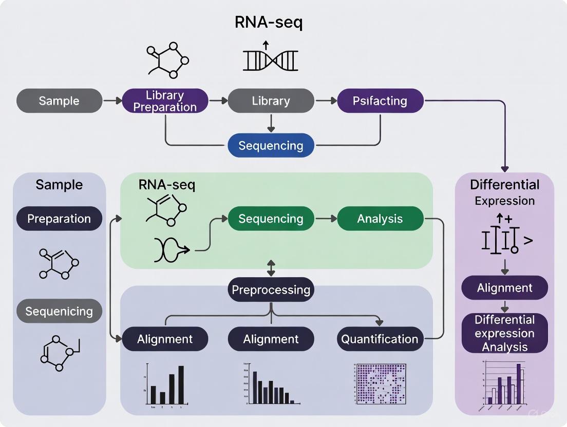
The primary goal of the initial RNA-seq data processing stage is to transform raw sequencing data into a gene count matrix, a table where rows represent genes, columns represent samples, and integer values indicate the number of sequencing reads assigned to each gene in each sample [1] [2]. This count matrix is the fundamental input for downstream statistical analyses, such as the identification of differentially expressed genes [3].

The journey begins after RNA has been extracted from biological samples, reverse-transcribed into complementary DNA (cDNA), and sequenced on a high-throughput platform [1]. The following diagram illustrates the core steps in this transformation process.

Detailed Methodologies for Core Workflow Steps

Primary Analysis: From BCL to FASTQ

The first computational step involves converting raw data from the sequencer into sequence reads.

• Base Calling and Demultiplexing: Sequencing instruments initially generate data in proprietary binary base call (BCL) formats. Using tools like bcl2fastq, these files are converted into standard FASTQ format files. During this process, demultiplexing is performed, where sequenced reads are sorted into individual sample-specific FASTQ files based on their unique index (barcode) sequences [4].
• FASTQ Format: The FASTQ file is the standard output, storing each read across four lines: a sequence identifier, the nucleotide sequence, a separator line, and a string of quality scores encoding the confidence of each base call [5] [2]. For paired-end sequencing, two FASTQ files (R1 and R2) are generated per sample.

Quality Control and Read Trimming

Assessing and cleaning the raw reads is crucial to ensure the reliability of subsequent analysis.

• Quality Control with FastQC: Tools like FastQC provide an initial overview of data quality, highlighting potential issues such as leftover adapter sequences, unusual base composition, or regions of low quality scores [1] [5]. This generates an HTML report for visual inspection.
• Read Trimming with Trimmomatic or Cutadapt: Based on the QC report, reads are cleaned using tools like Trimmomatic or Cutadapt. This step removes adapter sequences, trims low-quality bases from the ends of reads, and filters out very short reads [1] [5] [4]. This process improves the accuracy of read alignment in the next step.

Alignment and Quantification

This is the core step where reads are mapped to a reference to determine their genomic origin.

• Alignment-Based Workflow: In this traditional approach, cleaned FASTQ reads are aligned to a reference genome using "splice-aware" aligners such as STAR or HISAT2 [1] [5] [3]. These tools can handle reads that span intron-exon junctions. The output is typically in SAM/BAM format. The aligned reads are then counted per gene using tools like featureCounts, which produces the raw counts for the matrix [1] [5].
• Lightweight/Pseudoalignment-Based Workflow: As a faster and often more accurate alternative, tools like Salmon and Kallisto perform quantification directly from the FASTQ files without generating a full base-by-base alignment [1] [6] [2]. They use statistical models to rapidly estimate transcript abundances, incorporating uncertainty in read assignment. The output is a file of "pseudocounts" that can be aggregated into a gene-level count matrix.

Post-Alignment QC and Aggregated Reporting

A final quality check is performed before analysis.

• Post-Alignment QC: After alignment, tools like Qualimap analyze the BAM files to check for biases such as DNA or rRNA contamination, 5'-3' bias, and coverage uniformity across genes [2].
• Aggregated Reporting with MultiQC: When dealing with multiple samples, MultiQC is invaluable. It aggregates results from FastQC, Trimmomatic, Salmon, STAR, Qualimap, and others into a single HTML report, allowing for easy comparison of QC metrics across all samples [1] [2].

Key Data Formats and Normalization Techniques

Essential File Formats in RNA-seq

The workflow involves several standard file formats, each serving a distinct purpose.

Table 1: Key File Formats in the RNA-seq Processing Workflow

Format	Description	Primary Use Case
FASTQ [5] [2]	Stores nucleotide sequences and their corresponding per-base quality scores.	Output from demultiplexing; input for alignment/quantification tools.
SAM/BAM [1] [3]	SAM (Sequence Alignment Map) is a text-based format for aligned reads; BAM is its binary, compressed version.	Output from genome aligners like STAR and HISAT2.
Gene Count Matrix [1] [3]	A table where rows are genes, columns are samples, and values are raw integer counts of aligned reads.	The final output of the preprocessing workflow and primary input for differential expression analysis.

Common Normalization Methods

Raw count data must be normalized to remove technical biases before comparative analysis. Different methods correct for different factors.

Table 2: Common Normalization Methods for RNA-seq Count Data

Method	Sequencing Depth Correction	Gene Length Correction	Library Composition Correction	Suitable for DE Analysis
CPM [1]	Yes	No	No	No
RPKM/FPKM [1]	Yes	Yes	No	No
TPM [1]	Yes	Yes	Partial	No
Median-of-Ratios (DESeq2) [1]	Yes	No	Yes	Yes
TMM (edgeR) [1]	Yes	No	Yes	Yes

The Scientist's Toolkit: Essential Research Reagents and Software

A successful RNA-seq experiment relies on a combination of laboratory reagents and bioinformatics software.

Table 3: Essential Reagents and Software for RNA-seq Analysis

Category	Tool/Reagent	Function
Wet-Lab Reagents	Poly(dT) Oligos / Ribo-Zero	Enriches for mRNA by selecting polyadenylated transcripts or depleting abundant ribosomal RNA [7] [2].
	Fragmentation Enzymes/Reagents	Shears RNA or cDNA into uniform fragments of optimal size for sequencing [2].
	Reverse Transcriptase	Synthesizes first- and second-strand cDNA from the RNA template [2].
Core Bioinformatics Software	FastQC [5] [2]	Performs initial quality control checks on raw FASTQ files.
	Trimmomatic/Cutadapt [1] [5]	Trims adapter sequences and low-quality bases from reads.
	STAR/HISAT2 [1] [5] [3]	Aligns reads to a reference genome (splice-aware).
	Salmon/Kallisto [1] [6] [2]	Performs fast, alignment-free quantification of transcript abundances.
	featureCounts [1] [5]	Counts the number of reads mapping to each genomic feature (e.g., gene).
Quality Control & Visualization	Qualimap [1] [2]	Provides quality control metrics for aligned data in BAM files.
	MultiQC [1] [2]	Aggregates results from multiple tools and samples into a single report.
Downstream Analysis	DESeq2 / edgeR / limma [1] [3] [6]	Performs statistical testing for differentially expressed genes using the count matrix.

In the structured workflow of RNA-seq data analysis, the steps taken before sequencing—the experimental design—are arguably the most critical. They form the foundation upon which all subsequent computational analyses and biological conclusions are built. A poorly designed experiment can introduce biases and technical artifacts that even the most advanced statistical methods cannot later remedy [8]. As one perspective notes, consulting a statistician after an experiment is complete is often merely asking them "to conduct a post mortem examination... [to] say what the experiment died of" [8]. This guide details the core principles of experimental design—appropriate replication, strategic controls, and proactive management of batch effects—within the context of a complete RNA-seq research workflow. Adhering to these principles ensures that resources are used efficiently and that the resulting data provides a valid and reliable basis for scientific discovery, particularly in critical applications like drug development [9].

The Pillars of Sound Experimental Design

The reliability of any RNA-seq experiment rests on three key pillars: adequate replication to measure biological variability, appropriate controls to calibrate measurements, and careful design to minimize confounding technical noise.

Replication: Biological vs. Technical and Sample Size

Replication is fundamental for capturing the natural variation in biological systems and for assessing the reliability of observed effects. It is crucial to distinguish between the two primary types of replicates:

• Biological Replicates are independent biological samples (e.g., different individuals, animals, or separately cultured cell lines) representing the same experimental condition. They are essential for capturing biological variability and ensuring that findings are generalizable beyond the specific samples used [9].
• Technical Replicates involve multiple measurements of the same biological sample (e.g., splitting one RNA sample across multiple library preps or sequencing runs). They help assess technical variation introduced by the laboratory workflow but do not provide information about biological variability [9].

For most experiments aiming to make generalizable biological inferences, biological replication is the priority. While technical replicates can be useful for optimizing protocols, they cannot substitute for biological replicates [9].

Determining an adequate sample size is a critical step. An underpowered study, with too few biological replicates, is unlikely to detect genuine differential expression. Power analysis is a statistical method used to optimize sample size, balancing resource constraints with the need for reliable results [8]. While a common recommendation is a minimum of three biological replicates per condition, more may be needed for studies expecting subtle expression changes or working with highly variable samples [9]. Pilot studies are an excellent way to gather preliminary data on variability to inform sample size decisions for the main experiment [9].

Table 1: Types of Replicates in RNA-seq Experiments

Replicate Type	Definition	Purpose	Example
Biological Replicate	Independent biological samples or entities [9]	To assess biological variability and ensure findings are reliable and generalizable [9]	3 different animals or cell samples in each experimental group (treatment vs. control) [9]
Technical Replicate	The same biological sample, measured multiple times [9]	To assess and minimize technical variation (e.g., from sequencing runs or lab workflows) [9]	3 separate RNA sequencing experiments for the same RNA sample [9]

Controls: Positive, Negative, and Spike-Ins

Controls are reference points that allow researchers to validate their experimental protocols and interpret results correctly.

• Positive and Negative Controls: These are fundamental for verifying that an experiment worked as expected.
  • Positive controls are samples where a known effect is expected. For a drug treatment experiment, this could be a well-characterized compound known to induce a specific transcriptional response.
  • Negative controls are samples where no effect is expected. A common example is an "untreated" or "vehicle control" group, which is exposed to the solvent used to deliver a drug but not the active compound itself. Comparing treated samples to the appropriate negative control is essential for identifying drug-specific effects [9].
• Spike-in Controls: These are synthetic RNA sequences (e.g., SIRVs) added in known quantities to each sample at the start of the workflow. They serve as an internal standard to monitor the performance of the entire assay, including dynamic range, sensitivity, and quantification accuracy across samples and batches [9] [10]. They are particularly valuable for large-scale experiments to ensure data consistency and for normalizing samples where global transcript levels are expected to change [9].

Batch Effects: The Hidden Confounder

A batch effect is a systematic, non-biological variation introduced into data due to technical differences in sample processing [10]. These effects can arise from numerous sources, including different library preparation dates, reagent lots, personnel, or sequencing machines [10]. Even biologically identical samples processed in different batches can show significant differences in gene expression profiles, which can obscure true biological signals or create false positives [10] [11].

Table 2: Common Causes of Batch Effects in Transcriptomics

Category	Examples	Applies To
Sample Preparation	Different protocols, technicians, enzyme efficiency	Bulk & single-cell RNA-seq [10]
Sequencing Platform	Machine type, calibration, flow cell variation	Bulk & single-cell RNA-seq [10]
Library Prep Artifacts	Reverse transcription efficiency, amplification cycles	Mostly bulk RNA-seq [10]
Reagent Batches	Different lot numbers, chemical purity variations	All types [10]
Environmental Conditions	Temperature, humidity, handling time	All types [10]

The most reliable strategy for managing batch effects is to prevent them during experimental design. This involves:

• Randomization: Avoid processing all samples from one condition together. Instead, randomize the processing order of samples from all conditions across batches [8] [10].
• Balancing: Ensure that each biological group is represented within each processing batch. This prevents "confounding," where a technical batch is perfectly correlated with a biological condition, making it impossible to separate the two [8] [11].
• Metadata Tracking: Meticulously record all technical and processing information (dates, reagent lots, personnel, etc.) to use as covariates during statistical analysis [12].

When batch effects cannot be avoided, computational correction methods are required. Several tools are available, each with strengths and limitations.

Table 3: Common Batch Effect Correction Methods for Transcriptomics Data

Method	Strengths	Limitations
ComBat	Simple, widely used; adjusts known batch effects using an empirical Bayes framework [10] [13]	Requires known batch info; may not handle nonlinear effects well [10]
limma removeBatchEffect	Efficient linear modeling; integrates well with differential expression analysis workflows [10] [6]	Assumes known, additive batch effects; less flexible [10]
SVA (Surrogate Variable Analysis)	Captures hidden batch effects; suitable when batch labels are unknown [10]	Risk of removing biological signal; requires careful modeling [10]
Harmony	Effective for single-cell data; iteratively aligns cells in a shared embedding space [10] [11]	Designed for cell embeddings, not raw count matrices [10]

Integrating Design into the RNA-seq Workflow

A robust RNA-seq project is a multi-stage process, from hypothesis formulation to data interpretation. The following workflow diagrams illustrate how experimental design principles are integrated into the key wet-lab and computational phases.

Experimental Design and Wet-Lab Workflow

This diagram outlines the critical pre-sequencing steps where careful planning prevents future problems.

Computational Analysis with Batch Effect Management

This diagram maps the core bioinformatics steps, highlighting where batch effects are detected and corrected.

The Scientist's Toolkit: Essential Reagents and Materials

Successful execution of a well-designed RNA-seq experiment relies on key reagents and materials. The following table details critical components for generating high-quality libraries and data.

Table 4: Key Research Reagent Solutions for RNA-seq

Item	Function	Application Notes
Spike-in Controls (e.g., SIRVs)	Synthetic RNA sequences added to samples to monitor technical performance, normalization, and quantification accuracy [9] [10].	Essential for large-scale studies and experiments where global changes in transcript levels are expected [9].
RNA Extraction Kit	Isolates total RNA from biological material (cells, tissues, FFPE blocks) [9].	Must be selected based on sample type and the RNA species of interest (e.g., small RNAs) [9].
rRNA Depletion / mRNA Enrichment Kits	Enriches for coding RNA by removing abundant ribosomal RNA (rRNA) or selecting for polyadenylated mRNA [9].	Choice depends on the organism and study goals. rRNA depletion is often used for degraded samples (e.g., FFPE) [9].
Library Preparation Kit	Converts RNA into a sequence-ready DNA library. Includes reverse transcription, adapter ligation, and PCR amplification steps [9].	3'-end focused kits (e.g., QuantSeq) are cost-effective for large-scale gene expression studies, while whole transcriptome kits are needed for isoform analysis [9].
Strandedness Control Reagents	Reagents within the library prep kit that preserve the information about which DNA strand was the original RNA template [6].	Critical for accurately assigning reads to genes, especially in regions where genes overlap on opposite strands.

The path to robust and interpretable RNA-seq data begins long before the sequencing run. A rigorous experimental design, characterized by sufficient biological replication, thoughtfully selected controls, and proactive strategies to mitigate batch effects, is not an optional preliminary step but the very foundation of scientific validity. By integrating these principles into every stage of the research workflow—from the initial hypothesis to the final computational analysis—researchers can ensure their experiments yield meaningful biological insights, accelerate discovery, and make reliable contributions to the scientific record, particularly in high-stakes fields like drug development.

Quality control (QC) of raw sequencing reads represents the foundational first step in any RNA sequencing (RNA-seq) data analysis workflow. This initial assessment is crucial for identifying potential problems in sequencing data that could compromise downstream analysis results and biological interpretations. High-throughput sequencing data inevitably contains various artifacts, including adapter contamination, low-quality bases, and overrepresented sequences, which must be detected and addressed before proceeding with alignment and differential expression analysis. Within the broader context of RNA-seq methodology, rigorous QC serves as a essential checkpoint that ensures the reliability and reproducibility of subsequent findings, particularly in pharmaceutical development and clinical research applications where conclusions may inform drug discovery decisions.

The establishment of robust QC procedures has become increasingly important as RNA-seq technologies evolve and sample sizes expand. Batch effects and subtle technical biases can easily confound biological results if not detected early in the analysis process [14]. This technical guide provides a comprehensive framework for implementing quality assessment of raw sequencing reads using two complementary tools: FastQC for individual sample evaluation and MultiQC for aggregated project-level visualization. When properly integrated into RNA-seq workflows, these tools enable researchers to quickly identify problematic samples, make informed decisions about read processing parameters, and document quality metrics for regulatory compliance or publication purposes.

Theoretical Foundation: Sequencing Quality Metrics and Their Interpretation

Essential Quality Control Metrics

Quality assessment of high-throughput sequencing data relies on multiple complementary metrics that collectively provide a comprehensive picture of data quality. The most fundamental metrics include per-base sequence quality, which assesses Phred quality scores across all sequencing cycles; per-base sequence content, which examines nucleotide representation at each position; GC content distribution, which compares the observed GC distribution to a theoretical model; sequence duplication levels, which identify overrepresented sequences; and adapter contamination, which quantifies the presence of adapter sequences in read data [15] [16]. Each metric provides unique insights into different potential problems that could affect downstream analysis.

The interpretation of these metrics requires understanding both the sequencing technology employed and the biological system under investigation. For instance, certain sequence content biases are expected in RNA-seq data due to the non-random nature of transcript sequences, while other patterns may indicate technical artifacts requiring remediation. Similarly, the expected duplication level varies depending on sequencing depth and transcriptome complexity, with highly expressed genes naturally exhibiting higher duplication rates. Proper interpretation therefore necessitates considering both the technical context of library preparation and sequencing methodology alongside the biological context of the sample source [17].

Implications for Downstream Analysis

Quality issues undetected at the raw read stage can propagate through the entire analysis pipeline, potentially leading to erroneous biological conclusions. Adapter contamination can cause misalignment of reads to incorrect genomic locations, while systematic quality drops at read ends may reduce mapping rates and coverage uniformity. GC bias can skew expression estimates, particularly for genes with extreme GC content, and overrepresented sequences may indicate contamination that could compromise sample integrity interpretations [15]. These issues are particularly critical in drug development contexts, where inaccurate expression measurements could mislead target identification or biomarker discovery efforts.

The consequences of poor quality data extend beyond immediate analytical concerns to encompass resource allocation and experimental planning. Datasets with fundamental quality issues may be unsuitable for their intended purposes, necessitating costly resequencing and potentially delaying research timelines. Comprehensive initial QC provides the evidence base for these decisions, enabling researchers to distinguish between minor issues that can be addressed computationally and major problems requiring wet-lab intervention. This proactive approach to quality management ultimately enhances research efficiency and reliability across the RNA-seq workflow [17].

Experimental Protocols: Implementing FastQC and MultiQC

FastQC Analysis of Individual Samples

FastQC provides a comprehensive quality assessment of raw sequencing data through a series of modular analyses. The tool accepts input in various formats, including FASTQ, BAM, and SAM files, and generates both graphical summaries and text-based reports for each input file [15]. The implementation protocol begins with quality assessment of individual sequencing files before proceeding to multi-sample aggregation.

Step-by-Step Protocol:

• Tool Installation: FastQC requires Java Runtime Environment (JRE). Download the software from the Babraham Bioinformatics website and install according to platform-specific instructions [15].
• Basic Execution: For a single FASTQ file, use the command: fastqc sample.fastq.gz. This generates an HTML report and a ZIP file containing detailed data.
• Batch Processing: To process multiple files simultaneously: fastqc sample1.fastq.gz sample2.fastq.gz sample3.fastq.gz.
• Output Interpretation: Open the generated HTML file in a web browser to visualize quality metrics. Examine each module for warnings or failures that indicate potential quality issues.

FastQC provides multiple configuration options to customize analysis based on specific needs. The --nogroup option disables base grouping for long reads, providing higher resolution quality assessment. The --extract option automatically unzips output files, while --format allows explicit specification of file format when auto-detection fails [15]. For large-scale analyses, FastQC can be integrated into automated pipelines with results parsed from the text output files rather than manual inspection of HTML reports.

MultiQC for Aggregated Quality Reporting

MultiQC addresses the significant challenge of consolidating and comparing QC results across multiple samples by automatically scanning directories for analysis logs and generating unified reports [18] [14]. The tool recognizes output from numerous bioinformatics tools, with FastQC being one of its most prominently supported formats.

Step-by-Step Protocol:

• Tool Installation: Install MultiQC via Python Package Index using: pip install multiqc [14].
• Basic Execution: Navigate to the directory containing FastQC reports and execute: multiqc . (the dot indicates current directory). MultiQC will recursively search for recognized output files [19] [20].
• Output Customization: Use the --filename parameter to assign a custom name to the output report: multiqc --filename project_qc_report . [20].
• Report Interpretation: Open the generated HTML file to explore interactive plots and summary tables. Use the navigation menu to jump to specific sections and the toolbox to highlight samples of interest.

MultiQC provides numerous advanced options for handling complex project structures. The --dirs flag prefixes sample names with directory paths to distinguish between samples with identical names processed in different contexts. The --ignore option excludes specific files or patterns from analysis, while --file-list processes only explicitly listed files [20]. These features make MultiQC adaptable to diverse project organizations and naming conventions commonly encountered in large-scale RNA-seq studies.

Integrated Workflow for Comprehensive Quality Assessment

A robust quality assessment protocol combines both tools in a sequential workflow that provides both granular and holistic views of data quality. The integrated approach begins with individual file assessment using FastQC, proceeds to aggregated reporting with MultiQC, and culminates in informed decision-making about necessary quality remediation steps.

Table 1: FastQC Analysis Modules and Interpretation Guidelines

Module Name	Function	Potential Issues Detected	Interpretation Guidelines
Per-base sequence quality	Assesses Phred quality scores across all bases	Quality drops at read ends, consistently low quality	Scores below 20 indicate potential problems for variant calling
Per-base sequence content	Examines nucleotide proportion per cycle	Library-specific biases, random hexamer priming issues	First 10-15 bases often show bias in RNA-seq data
Per-sequence GC content	Compares observed vs. theoretical GC distribution	Contamination, PCR biases	Sharp peaks may indicate contamination; shifts suggest biases
Sequence duplication levels	Identifies overrepresented sequences	PCR over-amplification, low complexity libraries	High duplication in RNA-seq expected for highly expressed genes
Adapter content	Quantifies adapter sequence presence	Adapter contamination requiring trimming	Any significant adapter content (>1%) warrants trimming
Overrepresented sequences	Flags sequences with unexpected high frequency	Contaminants, PCR artifacts	BLAST significant hits to identify source

The output from this integrated workflow provides both detailed individual metrics and project-wide trends that inform subsequent processing steps. The General Statistics table in MultiQC reports provides a concise overview of key metrics across all samples, enabling rapid identification of outliers [18]. Interactive plots facilitate exploration of specific quality aspects, while the toolbox enables sample highlighting, renaming, and filtering to focus on specific sample subsets [18]. This comprehensive approach ensures that quality assessment captures both individual sample issues and systematic patterns affecting multiple samples.

Table 2: Essential Research Reagents and Computational Tools for Quality Assessment

Tool/Resource	Function	Application Context	Key Considerations
FastQC	Quality control analysis of raw sequencing data	Initial assessment of individual sequencing files	Java-dependent; multiple input format support
MultiQC	Aggregate results from multiple tools and samples	Project-level quality overview and comparison	Supports >50 bioinformatics tools; customizable output
Trim Galore	Adapter trimming and quality filtering	Read preprocessing based on QC results	Wrapper around Cutadapt and FastQC
Cutadapt	Adapter removal from sequencing reads	Specific adapter contamination issues	Precise adapter sequence specification required
fastp	Integrated QC and preprocessing	Streamlined workflow for large datasets	Performs filtering, trimming, and QC simultaneously
Reference genomes	Species-specific sequence databases	Context for contamination detection	Must match studied organism and assembly version

Successful quality assessment requires not only the primary analysis tools but also appropriate computational infrastructure. FastQC benefits from sufficient memory allocation, particularly for large datasets, with a --memory option available to control usage [15]. MultiQC efficiently handles projects with hundreds of samples, automatically switching to static plots for large sample numbers to maintain browser responsiveness [14]. For institutional sequencing facilities or large-scale drug development projects, MultiQC plugins enable integration with Laboratory Information Management Systems (LIMS) for automated metadata incorporation and result tracking [14].

Alternative tools offer complementary capabilities for specific use cases. Falco provides a high-speed FastQC emulation that generates equivalent results with improved performance, particularly valuable for high-throughput environments [21]. FastQ Screen extends quality assessment beyond technical metrics to sequence origin, detecting contamination from other species by mapping reads against multiple reference genomes [22]. These specialized tools can be incorporated into enhanced QC workflows when project requirements warrant additional checks.

Workflow Visualization and Implementation

The following diagram illustrates the integrated quality assessment workflow incorporating both FastQC and MultiQC:

Quality Assessment Workflow: This diagram illustrates the sequential process of raw read quality evaluation, highlighting the iterative nature of quality remediation when issues are detected.

The MultiQC reporting system generates interactive visualizations that enable researchers to explore quality metrics across multiple dimensions:

MultiQC Reporting Structure: This diagram outlines the internal processing steps within MultiQC, from log file parsing to the generation of interactive output reports with multiple visualization components.

Interpretation Guidelines and Decision Framework

Critical Metrics and Thresholds

Effective quality assessment requires not just metric calculation but also evidence-based interpretation against established thresholds. Based on empirical analyses of RNA-seq data, certain thresholds provide practical guidance for quality determinations. Per-base sequence quality should generally maintain Phred scores above 20 (99% base call accuracy) throughout most of the read, with minor degradation at the very ends often being tolerable for alignment [16]. Adapter content exceeding 1% typically warrants trimming intervention, while GC content deviations from the expected distribution may indicate contamination or other technical artifacts [15].

The interpretation must be contextualized to the specific experiment and sequencing technology. For instance, RNA-seq data naturally exhibits sequence content bias at the beginning of reads due to random hexamer priming artifacts, which would be flagged as problematic in genomic DNA but represents expected technical bias in transcriptomic data [16]. Similarly, duplication levels must be interpreted in light of sequencing depth and transcriptome diversity, with highly expressed genes expected to produce duplicate reads at appropriate levels. This nuanced interpretation prevents both undetected quality issues and unnecessary rejection of biologically valid data patterns.

Performance Considerations and Alternative Approaches

As sequencing projects grow in scale, computational efficiency of quality assessment becomes increasingly important. Performance comparisons indicate that Falco, a FastQC alternative implemented in C++, provides equivalent results with significantly faster execution times—approximately three times faster than FastQC while using less memory [21]. This performance advantage becomes substantial when processing large datasets or in high-throughput sequencing facilities where computational resource optimization is essential.

Alternative quality assessment tools offer different functionality trade-offs. Fastp provides an integrated solution that performs filtering, trimming, and quality control in a single step, with speed advantages particularly valuable for large-scale analyses [17]. However, FastQC remains the most widely adopted tool with the most comprehensive module coverage, making it particularly suitable for initial quality assessment in regulated environments where standardized methodologies are preferred. For most research applications, the combination of FastQC and MultiQC provides the optimal balance between comprehensive assessment and practical implementation.

Quality assessment of raw reads with FastQC and MultiQC represents the essential foundation upon which reliable RNA-seq analysis is built. This initial phase enables researchers to verify data quality, identify potential technical artifacts, and make informed decisions about necessary preprocessing steps before proceeding to alignment and expression quantification. The comprehensive visualization and aggregation capabilities of these tools facilitate both technical validation and documentation of quality metrics for publication or regulatory compliance.

When properly implemented within the broader RNA-seq workflow, this quality assessment phase serves as a critical checkpoint that safeguards downstream analyses from technical artifacts that could compromise biological interpretations. This is particularly crucial in drug development contexts, where decisions about target engagement or biomarker selection may hinge on accurate differential expression results. By establishing robust, reproducible quality assessment procedures using the methodologies outlined in this guide, researchers can ensure the reliability and interpretability of their RNA-seq analyses throughout subsequent computational and biological validation stages.

In RNA sequencing (RNA-seq) analysis, data cleaning through adapter trimming and quality filtering forms the essential foundation for all downstream biological interpretations. This process directly addresses the fundamental truth that raw sequencing data invariably contains artifacts that can compromise analytical integrity if left unaddressed. Without proper cleaning, researchers risk misalignment of reads, inaccurate quantification of gene expression, and ultimately, biologically misleading conclusions [23] [1].

Adapter contamination occurs when segments of the artificial sequences used during library preparation remain attached to the biological sequences of interest. This typically happens when DNA fragments are shorter than the read length, causing the sequencer to continue reading into the adapter sequence [24]. Simultaneously, sequencing quality naturally degrades along the length of reads, particularly at the 3' end, introducing base-calling errors [25]. The cleaning process systematically removes these technical artifacts while preserving biological signal, ensuring that the data passed to alignment and quantification tools represents actual transcript sequences rather than technical noise [26].

Within the broader RNA-seq workflow, data cleaning occupies a critical position immediately following initial quality assessment and preceding alignment [1]. This strategic placement ensures that aligners and quantifiers receive optimized input, leading to more accurate mapping, reduced computational resources, and ultimately, more reliable detection of differentially expressed genes [25] [26].

Key Concepts: Adapters, Quality Scores, and Filtering Criteria

Understanding Adapter Contamination

Adapter sequences are artificial oligonucleotides integrated during library preparation that enable the sequencing process. However, they become contaminants when they appear within the sequenced reads themselves. The most common scenario occurs with short RNA fragments where the read length exceeds the fragment length, resulting in the sequencer "reading through" the biological fragment and into the adapter sequence [24]. The resulting adapter contamination can manifest in several ways: as full adapter sequences within reads, partial adapter sequences at read ends, or in paired-end sequencing, as short adapter remnants forming "palindrome" sequences between forward and reverse reads [24].

Quality Metrics and Filtering Parameters

Sequencing quality is quantified using Phred quality scores (Q-score), which represent the probability that a base was called incorrectly [25]. A Q-score of 30 indicates a 1 in 1000 error probability (99.9% accuracy), which is typically considered the minimum threshold for high-quality data [25]. Effective filtering employs multiple criteria to eliminate problematic reads while preserving biological content:

• Minimum Length Threshold: Discards reads that become too short after trimming to contain meaningful mapping information (e.g., < 25-35 nucleotides) [27] [23].
• Quality Thresholds: Removes reads with overall poor quality or trims low-quality regions using sliding window approaches [24].
• Ambiguous Base Limits: Filters reads containing excessive 'N' characters representing uncertain base calls [23].
• Complexity Filtering: Eliminates reads with low sequence complexity (e.g., homopolymers) that may align unreliably [23].

Trimmomatic: A Versatile Processing Workhorse

Trimmomatic operates as a comprehensive trimming tool specifically designed for Illumina data, employing a multi-step processing pipeline to address various quality issues systematically [27] [24]. Its modular architecture allows researchers to combine different processing steps tailored to their specific data characteristics.

The tool's key advantage lies in its flexible handling of adapter contamination through the ILLUMINACLIP parameter, which simultaneously manages standard adapter removal and specialized palindrome clipping for paired-end data [27] [24]. This parameter requires multiple sub-parameters including the adapter file path, seed mismatches, palindrome clip threshold, and simple clip threshold, providing fine-grained control over the adapter detection process [27].

Cutadapt: Precision Adapter Trimming

Cutadapt specializes in finding and removing adapter sequences through sophisticated alignment algorithms that allow for error-tolerant matching [28] [29]. Its core functionality revolves around searching for adapter sequences with a user-defined error rate (default: 0.1 or 10%), enabling detection of adapters even when they contain sequencing errors or minor degradation [29].

A particular strength of Cutadapt is its comprehensive adapter typology, which recognizes that adapters can appear in different orientations and locations relative to the biological sequence [28]. The tool supports regular 3' adapters (-a), 5' adapters (-g), anchored adapters that must appear at read ends (^ for 5', $ for 3'), and non-internal adapters that allow partial matches only at sequence termini [28]. This specificity prevents over-trimming while ensuring complete adapter removal.

Comparative Analysis: Tool Selection Guide

Feature Comparison

Table 1: Comparative analysis of Trimmomatic and Cutadapt features and performance.

Feature	Trimmomatic	Cutadapt
Primary Strength	Comprehensive quality processing	Precise adapter removal
Adapter Detection	Sequence-based + palindrome clipping	Alignment with error tolerance
Quality Trimming	Sliding window, leading, trailing	Quality cutoff, NextSeq-specific
Paired-end Handling	Dedicated modes with separate outputs	Coordinated trimming with pair awareness
Performance	Moderate speed, good efficiency	Fast with multicore support (-j option)
Best Applications	RNA-seq, WGS, datasets needing broad quality control	Small RNA-seq, amplicon sequencing, targeted adapter removal
Key Parameters	ILLUMINACLIP, SLIDINGWINDOW, MINLEN	-a/-g adapters, -e error rate, -m minimum length
Limitations	Limited non-Illumina adapter support	Less comprehensive quality processing

Selection Guidelines

The choice between Trimmomatic and Cutadapt depends on experimental context and data characteristics. Trimmomatic excels when dealing with standard RNA-seq data requiring comprehensive quality control beyond just adapter removal [23]. Its integrated approach to quality trimming, adapter clipping, and length filtering makes it ideal for transcriptomic studies where overall read quality may be variable.

Cutadapt proves superior when working with specialized library types such as small RNA sequencing, where precise removal of specific adapters is paramount [23]. Its flexible adapter specification and support for multiple adapter types make it invaluable for protocols with complex adapter structures or when targeting only specific contaminants without altering other read regions.

For datasets suffering from severe adapter contamination, some practitioners employ both tools sequentially—first using Cutadapt for precise adapter removal followed by Trimmomatic for general quality control—though this approach requires careful parameterization to avoid over-trimming [30].

Experimental Protocols and Methodologies

Trimmomatic Protocol for RNA-Seq Data

A standard Trimmomatic workflow for paired-end RNA-seq data incorporates multiple processing steps designed to address the most common data quality issues:

• ILLUMINACLIP: Removes adapter sequences using a reference adapter file with optimized parameters for sensitivity and specificity ILLUMINACLIP:TruSeq3-PE.fa:2:30:10 [24].
• SLIDINGWINDOW: Performs quality-based trimming using a sliding window approach SLIDINGWINDOW:5:10 (window size: 5 bases, required quality: 10) [24].
• LEADING/TRAILING: Removes low-quality bases from read starts and ends LEADING:5 TRAILING:5 [24].
• MINLEN: Filters reads that become too short after processing MINLEN:50 [24].

The complete command implementation appears as:

This protocol typically processes reads in a paired-end mode that maintains read synchronization, outputting both paired reads (where both mates survived filtering) and unpaired reads (where one mate was discarded) [24]. The ILLUMINACLIP step is particularly crucial for RNA-seq data, as it eliminates adapter sequences that could otherwise prevent accurate alignment to splice junctions.

Cutadapt Protocol for Precision Trimming

For targeted adapter removal in applications like small RNA sequencing, Cutadapt implements a focused approach:

• Adapter Specification: Define the exact adapter sequence and type based on library preparation method -a ADAPTER for 3' adapters [28].
• Error Tolerance: Set appropriate error rates balancing sensitivity and specificity -e 0.1 allows 10% errors in adapter matching [29].
• Quality Filtering: Apply quality thresholds and length filters -q 20 -m 15 [30].
• Parallel Processing: Utilize multicore support for efficiency -j 0 auto-detects available cores [29].

A typical Cutadapt command for removing Illumina universal adapters demonstrates this approach:

For paired-end data, the command expands to coordinate trimming between mates:

A critical consideration when using Cutadapt is adapter sequence specification. Research indicates that using the exact adapter sequence referenced by quality control tools like FastQC (sometimes shorter than manufacturer-provided sequences) significantly improves removal efficiency [30].

Integration within the RNA-Seq Workflow

Position in Analytical Pipeline

Data cleaning occupies a defined position in the comprehensive RNA-seq analytical workflow, situated between initial quality assessment and alignment/quantification steps. The complete pathway encompasses:

Diagram 1: RNA-seq workflow with trimming step highlighted.

This sequencing demonstrates how data cleaning bridges the gap between raw data generation and biological interpretation. The process typically begins with FastQC analysis of raw reads to identify specific quality issues, informs parameter selection for trimming tools, and concludes with post-cleaning verification to ensure successful artifact removal before proceeding to computationally intensive alignment steps [25] [1].

Quality Control Verification

Effective data cleaning requires quality verification at multiple stages. Initial FastQC reports on raw data identify adapter contamination levels, sequence quality degradation patterns, and other artifacts that inform trimming parameter selection [27]. Following trimming, a second FastQC analysis confirms the successful removal of adapters and quality improvement [27].

Key metrics to evaluate include:

• Adapter Content: Should approach 0% after successful trimming [27]
• Per Base Sequence Quality: Should show improved scores, particularly at 3' ends
• Sequence Length Distribution: Should reflect the minimum length threshold applied

For large-scale studies with multiple samples, MultiQC aggregates these metrics across all samples, enabling researchers to identify outliers and verify consistency throughout the dataset [25].

Table 2: Key reagents, tools, and their functions in RNA-seq data cleaning.

Resource	Function	Application Context
Trimmomatic	Comprehensive read trimming	General RNA-seq quality control
Cutadapt	Precision adapter removal	Small RNA-seq, targeted trimming
FastQC	Quality control assessment	Pre- and post-trimming validation
TruSeq3 Adapters	Standard Illumina adapter sequences	Reference for adapter contamination
MultiQC	Aggregate QC reporting	Multi-sample experiment validation
High-Quality RNA Samples	Starting material for sequencing	Foundation for all downstream steps
RIN > 7	RNA Integrity Number threshold	Sample quality verification pre-seq
Qubit/Bioanalyzer	Nucleic acid quantification and QC	Library preparation quality assurance

Impact on Downstream Analysis

Proper data cleaning exerts a profound influence on all subsequent analytical stages in the RNA-seq workflow. Alignment rates typically improve significantly after trimming, as reads devoid of adapter sequences and low-quality bases map more reliably to reference transcriptomes [23]. This enhanced mapping efficiency directly translates to more accurate gene-level quantification, as reads are assigned to their correct transcriptional origins rather than misaligning due to adapter contamination or quality issues.

The ultimate impact emerges in differential expression analysis, where cleaned data demonstrates improved detection power for genes with low to moderate expression levels [26]. Research has shown that appropriate cleaning methods can significantly increase the number of detected differentially expressed genes while providing more significant p-values, without introducing bias toward low-count genes [26]. This enhancement proves particularly valuable for identifying biologically relevant but weakly expressed transcripts that might otherwise be lost in technical noise.

Furthermore, effective cleaning reduces false positive variant calls in genomic studies, improves transcript assembly completeness, and increases the reproducibility of results across technical replicates [23]. By investing computational resources in thorough data cleaning, researchers establish a foundation of analytical integrity that supports all subsequent biological interpretations and conclusions derived from their RNA-seq experiments.

Within the RNA-seq data analysis workflow, the steps of selecting, annotating, and indexing a reference genome are foundational. The quality and appropriateness of these references directly determine the accuracy of all subsequent analyses, from read mapping and quantification to the final identification of differentially expressed genes. This guide provides researchers and drug development professionals with a technical roadmap for these critical initial steps, framed within the context of a complete RNA-seq research thesis.

Reference Genome Selection

Selecting an appropriate reference genome is the first and most critical choice in an RNA-seq study. Using an unsuitable reference can introduce mapping errors and systematic biases, compromising the entire project.

Official Selection Criteria

For species with established genomic resources, reference genomes are often formally designated by authoritative databases. The National Center for Biotechnology Information (NCBI) RefSeq database, for instance, selects a single "reference" genome for each defined species to provide a normalized, taxonomically diverse view of its collection [31].

The criteria for selection differ between prokaryotes and eukaryotes, with a summary of key metrics provided in Table 1.

Table 1: Key Criteria for Reference Genome Selection

Organism Type	Primary Criteria	Additional Considerations
Prokaryotes [31]	- Assembly contiguity (scaffold count)- CheckM completeness score- Low count of pseudo CDSs- Deviation from mean species assembly length	- Manual selection based on community input- Presence of plasmid sequences- Type strain status
Eukaryotes [31]	- Contig N50 value- Assembly completeness (gapless chromosomes, full chromosome set)	- Manual curation for high-profile species (e.g., human)- Preference for existing RefSeq genomes

For prokaryotes, the process is highly automated, weighing factors like assembly contiguity, gene completeness, and annotation quality [31]. For eukaryotes, the decision is often more nuanced, considering the contiguity of the assembly (e.g., contig N50) and its completeness, such as whether it possesses a full set of gapless chromosomes [31]. In some cases, manual selection overrides computational rankings, particularly for well-studied model organisms where a specific genome build has become the community standard [31].

Practical Selection for RNA-seq

When initiating an RNA-seq study, researchers should first seek out these officially designated reference genomes from databases like NCBI RefSeq or GENCODE [32]. If multiple options exist, the selection hierarchy for eukaryotes should be followed, prioritizing more contiguous and complete assemblies [31].

In the absence of a designated reference, such as for a non-model organism, the guiding principle is to select the assembly with the highest quality and most comprehensive gene annotation. It is also crucial to ensure that the genome sequence file (FASTA) and the annotation file (GTF/GFF) are from the same source and version to avoid coordinate mismatches [33].

Genome Annotation

Genome annotation is the process of inferring the structure and function of genomic sequences, identifying the locations of genes, exons, splice sites, and other functional elements. Accurate annotation is essential for correctly assigning RNA-seq reads to the genes from which they originated.

Annotation Methodologies

Annotation strategies have evolved from relying on single sources of evidence to integrated, evidence-driven pipelines.

• Ab Initio Prediction: Tools like AUGUSTUS use computational models to predict gene structures based on statistical signatures in the DNA sequence, such as codon usage and splice site patterns [34]. These are useful when experimental data is scarce but can have high false positive rates [35].
• Evidence-Based Annotation: This more accurate method leverages experimental data. Transcriptome data (e.g., from RNA-seq) is mapped to the genome to directly define exon-intron structures using assemblers like StringTie [35]. Protein sequences from related species can also be aligned to the genome to identify conserved coding regions [35].
• Integrated Annotation Pipelines: Modern pipelines like MAKER and BRAKER combine multiple lines of evidence—including ab initio predictions, transcriptomic alignments, and protein homology—to generate a consolidated and more accurate annotation [35] [34]. They use algorithms like EvidenceModeler to weigh and combine evidence into a final gene set [35].

Emerging Technologies: DNA Foundation Models

A transformative new approach frames genome annotation as a multilabel semantic segmentation task. Models like SegmentNT are built by fine-tuning pre-trained DNA foundation models, such as the Nucleotide Transformer, on known genomic elements [34].

These models can process long DNA sequences (up to 50 kb) and simultaneously predict the location of diverse genic and regulatory elements—including exons, introns, promoters, and enhancers—at single-nucleotide resolution [34]. This end-to-end methodology shows state-of-the-art performance and strong generalization across species, representing a significant advance over traditional pipeline-based methods [34].

The following diagram illustrates the conceptual workflow of this approach.

_{Diagram 1: Foundation model-based annotation workflow.}

Genome Indexing for RNA-seq

Before RNA-seq reads can be mapped, the reference genome and its annotation must be indexed. This process creates auxiliary files that allow the aligner to quickly and efficiently find potential mapping locations for each read, drastically reducing computation time.

Purpose of Indexing

Indexing creates a searchable catalog of all subsequences (e.g., k-mers) in the genome. For splicing-aware aligners like STAR, the process also incorporates the genome annotation to create a database of known splice junctions. This allows the aligner to recognize reads that span an intron, a critical feature for accurate transcriptome mapping [33].

Indexing with STAR

STAR (Spliced Transcripts Alignment to a Reference) is a widely used aligner for RNA-seq data. The following protocol details the steps for building a genome index.

Experimental Protocol: Building a Genome Index with STAR

Objective: To generate a genome index file for use with the STAR RNA-seq aligner. Inputs:

• Genome sequence in FASTA format (e.g., GRCh38.primary_assembly.genome.fa).
• Genome annotation in GTF format (e.g., gencode.v29.annotation.gtf).

Method:

• Data Preparation: Download the genome FASTA and GTF files from a trusted source like GENCODE, Ensembl, or UCSC, ensuring the versions match [33]. Unzip the files if necessary.
• Load Software Module: On a high-performance computing (HPC) cluster, load the STAR module (e.g., module load star).
• Run GenomeGenerate: Execute the STAR command in genomeGenerate mode. A typical command is shown below [33]:

Key Parameters:

• --genomeDir: Path to the directory where the index will be saved.
• --genomeFastaFiles: Path to the input genome FASTA file.
• --sjdbGTFfile: Path to the annotation GTF file for splice junction information.
• --sjdbOverhang: A critical parameter specifying the length of the genomic sequence around annotated junctions. This should be set to ReadLength - 1. For 100bp paired-end reads, use 99 [33].
• --runThreadN: Number of CPU threads to use for faster indexing.

Output: A directory containing the genome index files (e.g., chrLength.txt, Genome, SAindex).

The Scientist's Toolkit

Successful execution of a genome-based RNA-seq study requires a suite of key reagents and software tools. Table 2 details these essential components.

Table 2: Research Reagent and Tool Solutions for Reference-Based RNA-seq

Item	Function	Example Tools/Databases
Reference Genome (FASTA)	The DNA sequence of the organism used as a map for read alignment.	NCBI RefSeq [31], GENCODE [32], Ensembl
Genome Annotation (GTF/GFF)	File containing the coordinates and metadata for genes, transcripts, and other features.	GENCODE [32], Ensembl, NCBI
Splicing-aware Aligner	Software that aligns RNA-seq reads to a genome, accounting for introns.	STAR [33], HISAT2, minimap2 (long reads) [33]
Alignment-based Quantifier	Tool that estimates gene/transcript abundance from aligned reads.	Salmon (alignment mode) [6], featureCounts
Pseudo-aligner	Tool that rapidly estimates abundance by matching reads to a transcriptome without full alignment.	Kallisto [36], Salmon (standard mode) [6]
Integrated Workflow	Frameworks that automate multi-step RNA-seq analysis from raw data to counts.	nf-core/rnaseq [6]

The overall workflow for an RNA-seq experiment, from raw data to differential expression, is summarized in the diagram below.

_{Diagram 2: RNA-seq workflow with reference preparation highlighted.}

The processes of genome selection, annotation, and indexing form the critical foundation of a robust RNA-seq analysis. By understanding the official criteria for genome selection, leveraging integrated and modern deep learning-based annotation methods, and correctly implementing indexing protocols, researchers can ensure that their downstream differential expression and functional analysis results are built upon a reliable and accurate base. Mastery of these initial steps is indispensable for generating biologically meaningful and reproducible insights in genomics and drug development research.

From Alignment to Discovery: A Step-by-Step Analytical Pipeline

In RNA sequencing (RNA-Seq) analysis, the step of determining where sequencing reads originate from in the genome is fundamental to connecting genomic information with phenotypic and physiological data [37]. The choice of alignment strategy directly impacts the accuracy, efficiency, and biological validity of downstream results, including differential gene expression analysis. Currently, two predominant computational approaches exist: traditional spliced aligners (e.g., STAR, HISAT2) that perform base-by-base alignment to a reference genome, and modern pseudo-aligners (e.g., Salmon, Kallisto) that use fast k-mer matching to a reference transcriptome for quantification without exact positional alignment [38]. This technical guide provides an in-depth comparison of these strategies, supported by quantitative benchmarking data and detailed protocols, to inform researchers and drug development professionals in selecting optimal workflows for their specific research contexts.

Core Concepts: Fundamental Differences Between Alignment Strategies

Spliced Aligners: Genome-Based Mapping

Spliced aligners are designed to address the unique challenges of RNA-seq data mapping, particularly the presence of introns that cause reads to span splice junctions.

• STAR (Spliced Transcripts Alignment to a Reference) utilizes a novel strategy based on sequential maximum mappable seed search followed by clustering, stitching, and scoring stages [39]. For every read, STAR searches for the longest sequence that exactly matches one or more locations on the reference genome (Maximal Mappable Prefixes). These "seeds" are then stitched together based on proximity and alignment scoring to generate complete read alignments, including those spanning splice junctions [39].

• HISAT2 (Hierarchical Indexing for Spliced Alignment of Transcripts 2) employs a different approach using a graph-based alignment with a Ferragina-Manzini index (also used by bowtie2) that can align reads to a genome while being aware of splice sites [37]. This hierarchical indexing strategy allows efficient mapping against both small genomic regions and the entire genome.

Pseudo-aligners: Transcriptome-Based Quantification

Pseudo-aligners represent a paradigm shift in RNA-seq analysis by focusing directly on quantification while bypassing the computationally expensive step of base-by-base alignment.

• Kallisto introduces the concept of pseudo-alignments based on k-mer matching in a transcript De Bruijn graph. Rather than determining exact genomic positions, it establishes a relationship between a read and a set of compatible transcripts, then uses equivalence classes for rapid isoform quantification [37].

• Salmon utilizes a similar approach called quasi-mapping, which employs an indexed suffix array and Burrows-Wheeler Transform to discover shared substrings of any length between a read and transcript sequences [37]. It incorporates additional statistical modeling to correct for GC and sequence biases during quantification.

Table 1: Fundamental Operational Differences Between Alignment Tools

Feature	STAR	HISAT2	Salmon	Kallisto
Reference Type	Genome	Genome	Transcriptome	Transcriptome
Alignment Strategy	Seed extension & stitching [39]	Hierarchical FM-index [37]	Quasi-mapping [37]	Pseudo-alignment [37]
Splice Junction Handling	Direct detection via segmented alignment [39]	Graph-based alignment [37]	Not applicable	Not applicable
Primary Output	Genomic coordinates (BAM) [38]	Genomic coordinates (BAM) [38]	Transcript abundance [38]	Transcript abundance [38]
Key Innovation	Speed through uncompressed suffix arrays [39]	Memory efficiency through hierarchical indexing [40]	Bias correction & quasi-mapping [37]	k-mer matching in De Bruijn graph [37]

Quantitative Performance Comparison: Benchmarking Studies and Results

Mapping Efficiency and Concordance

Multiple studies have systematically compared the performance of different RNA-seq alignment tools. A 2020 evaluation of seven alignment tools on Arabidopsis thaliana data found that between 92.4% and 99.5% of reads were successfully mapped across different tools, with STAR achieving the highest mapping rates (99.5% for Col-0 and 98.1% for N14 accessions) [37]. The raw count distributions generated by different mappers showed high correlation, with coefficients ranging from 0.977 to 0.997 for Col-0 samples [37]. Notably, the highest similarity was observed between the pseudo-aligners kallisto and salmon (Rv = 0.9999) [37].

Differential Gene Expression Concordance

When assessing the impact on downstream differential expression analysis, studies reveal substantial but incomplete overlap between tools. Research on checkpoint blockade-treated CT26 experimental data showed that while all methods identified a core set of differentially expressed genes, HISAT2 detected additional unique genes not found by the pseudo-aligners [41]. The overlap of differentially expressed genes between kallisto and salmon was notably high (98%), while the lowest overlaps were detected between bwa and STAR (93.4%) [37].

Table 2: Performance Benchmarking Across Alignment Tools (Based on Multiple Studies)

Performance Metric	STAR	HISAT2	Salmon	Kallisto
Mapping Rate (%)	99.5 [37]	95-98 [37]	95-98 [37]	95-98 [37]
DGE Overlap with Salmon (%)	92-94 [37]	92-94 [37]	-	97-98 [37]
Small RNA Quantification	Accurate [42]	Accurate [42]	Reduced accuracy [42]	Reduced accuracy [42]
Resource Requirements	High memory [39]	Moderate [40]	Low [38]	Low [38]
Speed	Fast but memory-intensive [39]	Moderate [40]	Very fast [38]	Very fast [38]

Performance with Specialized RNA Types

Important performance differences emerge when quantifying specific RNA classes. A comprehensive 2018 study revealed that alignment-based pipelines significantly outperformed alignment-free tools for quantifying small structured non-coding RNAs (e.g., tRNAs, snoRNAs) and lowly-expressed genes [42]. While all pipelines showed high accuracy for quantifying protein-coding genes and synthetic spike-ins, alignment-free tools showed systematically poorer performance for small RNAs, particularly those containing biological variations [42].

Practical Implementation: Protocols and Workflow Integration

STAR Alignment Protocol

For researchers implementing STAR alignment, the following protocol provides a robust starting point:

Genome Index Generation:

Read Alignment:

This two-step process first creates a genome index optimized for the specific read length (--sjdbOverhang should be set to read length -1), then performs the actual read alignment, producing sorted BAM files ready for downstream quantification [39].

Pseudo-alignment Protocol with Salmon

For pseudo-alignment-based quantification, the workflow with Salmon typically involves:

Transcriptome Indexing:

Quantification:

This approach directly generates transcript abundance estimates in a fraction of the time required by traditional alignment [38].

Integrated workflows

Comprehensive RNA-seq pipelines like nf-core/RNA-seq support multiple alignment strategies, allowing researchers to choose between STAR, HISAT2, or pseudo-aligners based on their specific needs [40]. The pipeline also includes automated strandedness detection using Salmon quantification when set to 'auto', demonstrating how these tools can be complementary rather than mutually exclusive [40].

Table 3: Essential Computational Reagents for RNA-seq Alignment

Resource Type	Specific Examples	Function & Importance
Reference Genome	GRCh38 (Ensembl), HG38 (UCSC), GRCm39 (Mouse)	Baseline genomic sequence for alignment; must match annotation source [43]
Gene Annotation	GTF/GFF files from Ensembl, GENCODE, RefSeq	Provides transcript models for read assignment and quantification [43]
Alignment Indices	STAR genome index, HISAT2 index, Salmon transcriptome index	Pre-built structures enabling rapid read mapping [39]
Quality Control Tools	FastQC, MultiQC, RSeQC	Assess read quality, library complexity, and strandedness [40] [17]
Quantification Tools	featureCounts, HTSeq-count, tximport	Convert alignments to count data for differential expression [5]
Differential Expression	DESeq2, edgeR, limma-voom	Statistical analysis of expression changes between conditions [37]

Strategic Recommendations: Selecting the Right Tool for Your Research Context

Decision Framework for Alignment Strategy Selection

Based on comprehensive benchmarking studies and practical considerations, the following strategic recommendations emerge:

• For comprehensive transcriptome characterization including novel transcript discovery, alternative splicing analysis, or identification of genetic variants, traditional spliced aligners like STAR or HISAT2 remain essential [38]. These tools provide the genomic context necessary for such analyses, which pseudo-aligners cannot deliver.

• For standardized differential expression analyses focused on well-annotated protein-coding genes, pseudo-aligners offer an excellent combination of speed and accuracy [37] [38]. Their quantification performance for common gene targets is highly concordant with traditional aligners while offering substantial computational efficiency gains.

• For specialized applications involving small RNAs or other structured non-coding RNAs, alignment-based approaches currently demonstrate superior performance [42]. The k-mer-based approaches used by pseudo-aligners struggle with the unique characteristics of these RNA classes.

• In resource-constrained environments or for rapid iterative analysis, pseudo-aligners provide significant advantages, with kallisto demonstrating 2.6 times faster processing and 15x lower memory usage compared to STAR in single-cell RNA-seq benchmarks [38].

Emerging Trends and Future Directions

The distinction between alignment strategies is becoming increasingly blurred with tool development. Modern versions of Salmon incorporate "selective alignment," which represents a hybrid approach between traditional alignment and quasi-mapping [38]. Integrated workflows like nf-core/RNA-seq now support multiple alignment strategies within a single framework, allowing researchers to select the optimal approach based on their specific biological questions and computational resources [40].

Furthermore, recent research emphasizes that optimal tool selection should consider species-specific differences, with different analytical tools demonstrating performance variations when applied to data from humans, animals, plants, and fungi [17]. This highlights the importance of context-aware pipeline design rather than one-size-fits-all solutions in RNA-seq analysis.

Within the comprehensive workflow of RNA-seq data analysis, the steps following read alignment are critical for transforming raw sequencing data into biologically interpretable information. Post-alignment processing, encompassing file sorting, indexing, and rigorous quality control (QC), serves as the foundation for all subsequent analyses, including differential expression and pathway analysis [44]. Neglecting these steps can lead to incorrect biological interpretations, low reproducibility, and ultimately, wasted resources [45]. This guide details the essential procedures for processing alignment files using SAMtools and performing advanced quality assessment with Qualimap, providing a robust framework for researchers and drug development professionals to validate their data before proceeding to higher-order analyses.

Understanding the Alignment File Format: SAM/BAM

The Sequence Alignment/Map (SAM) format is a standardized, tab-delimited text file containing all alignment information for each read, while its binary equivalent (BAM) provides a compressed, computationally efficient representation of the same data [46] [47]. The BAM format is significantly smaller in size and is typically the required input for downstream tools [47].

A SAM/BAM file consists of two primary sections:

• Header Section: Optional, begins with the '@' character, and describes the source of data, reference sequence, and alignment method [46].
• Alignment Section: Each line corresponds to a single read and contains 11 mandatory fields that detail the essential mapping information [46].

Table 1: Mandatory Fields in a SAM/BAM File Alignment Record

Field Position	Field Name	Description
1	QNAME	Query template name (read identifier)
2	FLAG	Bitwise flag encoding various mapping properties
3	RNAME	Reference sequence name (chromosome)
4	POS	1-based leftmost mapping position
5	MAPQ	Mapping quality (phred-scaled probability of incorrect alignment)
6	CIGAR	String encoding alignment matches, mismatches, indels, and splices
7	MRNM	Mate reference sequence name (for paired-end reads)
8	MPOS	1-based leftmost mate position
9	ISIZE	Inferred insert size
10	SEQ	Read sequence
11	QUAL	Base quality scores (ASCII-encoded Phred values)

The FLAG field is of particular importance as it provides crucial information about the alignment in a bitwise format. Common flag values include 1 (read is paired), 2 (read is mapped in a proper pair), 4 (read is unmapped), and 16 (read aligns to the reverse strand) [46]. The CIGAR (Compact Idiosyncratic Gapped Alignment Report) string details the alignment by specifying the number and type of operations (e.g., M for match, I for insertion, D for deletion, N for skipped region) required to match the read to the reference [46]. This is especially critical for RNA-seq data as the 'N' operation can indicate the presence of a splice junction.

Essential SAM/BAM Processing with SAMtools

SAMtools is a versatile suite of utilities that enables efficient manipulation and analysis of SAM/BAM files [48]. Its functions include format conversion, sorting, indexing, filtering, and statistical summary generation.

Basic SAMtools Operations

The first steps typically involve converting between SAM and BAM formats, and sorting the alignments by genomic coordinate, which is a prerequisite for many downstream analyses.

Converting SAM to BAM and Sorting:

Indexing the Sorted BAM File: Indexing creates a separate index file (.bai) that allows for rapid retrieval of alignments from specific genomic regions without processing the entire file [48]. This is essential for visualization in genome browsers like IGV and for many quantification tools.

Filtering and Assessing Alignments

SAMtools provides powerful options for filtering alignments based on specific criteria and for generating basic mapping statistics.

Filtering by Mapping Quality: Removing poorly mapped or non-uniquely mapped reads can improve the reliability of downstream analysis.

It is crucial to understand that Mapping Quality (MAPQ) scores are calculated differently by various aligners. For example, STAR may output MAPQ values of 0, 1, 3, or 50, where 50 represents a unique match, while other aligners like Bowtie2 have a different scoring range [48].

Filtering with SAM Flags: SAM flags can be used to include (-f) or exclude (-F) reads based on specific alignment characteristics.

Generating Mapping Statistics: The flagstat command provides a quick overview of the mapping performance.

Table 2: Key SAMtools Commands for Post-Alignment Processing

Command	Function	Common Usage
samtools view	Format conversion, read filtering, and region extraction	samtools view -b -h input.sam > output.bam
samtools sort	Sorts alignments by genomic coordinate	samtools sort input.bam -o output_sorted.bam
samtools index	Creates an index for a sorted BAM file	samtools index sorted_input.bam
samtools flagstat	Generates simple statistics from the BAM file	samtools flagstat input.bam
samtools idxstats	Reports alignment statistics per reference sequence	samtools idxstats input.bam

The following workflow diagram outlines the logical sequence of these core SAMtools processing steps:

Figure 1: Core SAMtools Data Processing Workflow

Comprehensive Quality Control with Qualimap

After processing BAM files with SAMtools, the next critical step is an in-depth quality assessment. Qualimap is a Java application that generates comprehensive QC reports for NGS data, including specific modules for RNA-seq [47] [49].

Running Qualimap RNA-seq QC

Qualimap requires a sorted and indexed BAM file, along with an annotation file in GTF format.

Basic Qualimap Command:

Key Input Parameters:

• -bam: Path to the input sorted BAM file.
• -gtf: Annotation file in GTF format.
• -outdir: Directory to store the HTML report and output files.
• --java-mem-size: Memory allocated to the Java engine (important for large files).
• -pe: Option for paired-end data.
• -s: Strand-specific library protocol (e.g., -s strand-specific-forward).

Interpreting Key Qualimap Output and Metrics

The Qualimap HTML report provides multiple sections with diagnostic plots and metrics. For RNA-seq data, several aspects are particularly important for assessing technical quality [47] [49].

Reads Genomic Origin: This analysis determines the proportion of reads mapping to exonic, intronic, and intergenic regions. A high-quality RNA-seq sample typically shows a majority of reads (e.g., >55%) mapping to exonic regions. An unusually high number of reads in intronic regions (>30%) may indicate significant genomic DNA contamination or a high level of pre-mRNA [46].

Junction Analysis: Qualimap analyzes splice junctions, categorizing them as known, novel, or partly known. This provides insight into the transcriptomic complexity of the sample and the performance of the splice-aware aligner.

Transcript Coverage and 5'-3' Bias: Ideal transcript coverage should be relatively uniform from the 5' to 3' end. A significant coverage drop-off at either end indicates bias, potentially introduced during library preparation (e.g., RNA degradation or fragmentation issues). Qualimap calculates a 5'-3' bias value, where a value near 1 indicates minimal bias.

Strand Specificity: For strand-specific protocols, Qualimap assesses the success of strand preservation by reporting the percentage of reads aligning to the correct strand. A well-performing library will show values around 99% for the correct strand, whereas a non-strand-specific protocol will show roughly 50%/50% distribution [46].

Table 3: Critical RNA-seq QC Metrics from Qualimap and Their Interpretation

QC Metric	Target/Expected Value	Potential Issue if Outside Target
Exonic Rate	> 55%	DNA contamination or immature transcripts if low
Intronic Rate	< 30%	DNA contamination or immature transcripts if high
Intergenic Rate	< 10%	DNA contamination or incorrect annotation if high
rRNA Mapping Rate	< 2%	Inadequate rRNA depletion during library prep if high [46]
5'-3' Bias	~ 1.0	Library preparation bias or RNA degradation if deviated
Strand Specificity	~ 99% or ~ 1%	Failed strand-specific protocol if near 50%/50%
Junction Analysis	High proportion of known junctions	Many novel junctions may indicate poorly annotated transcriptome

The following diagram illustrates the interconnected nature of these QC metrics and the potential issues they reveal:

Figure 2: Qualimap RNA-seq QC Analysis and Diagnostic Pathways

The Scientist's Toolkit: Essential Research Reagents and Software

A successful RNA-seq post-alignment analysis relies on a combination of robust software tools and curated genomic resources. The following table details the essential components.

Table 4: Essential Research Reagents and Software Solutions for Post-Alignment QC

Item Name/Software	Type	Primary Function in Workflow
SAMtools	Software Suite	Core utility for processing, filtering, sorting, and indexing SAM/BAM files [46] [48].
Qualimap	Software Application	Generates comprehensive QC reports with RNA-seq specific metrics from aligned reads [47] [49].
Picard Tools	Software Suite	Provides additional QC functions like CollectRnaSeqMetrics for duplication rates and insert size distributions [50] [45].
Reference Genome	Data Resource	The genomic sequence (e.g., GRCh38 for human) used for alignment; must match the aligner's index.
Annotation File (GTF)	Data Resource	File containing genomic coordinates of genes, transcripts, and exons; essential for assigning reads to features and for Qualimap analysis [47] [49].
RSeQC	Software Suite	Optional tool providing additional RNA-seq specific QC, such as gene body coverage and junction saturation analysis [50].

Post-alignment processing with SAMtools and Qualimap represents a critical quality gateway in the RNA-seq analysis workflow. The meticulous steps of sorting, indexing, and comprehensive QC are not merely technical formalities but are fundamental to ensuring the biological validity and reproducibility of subsequent findings. By systematically applying the protocols and metrics outlined in this guide, researchers can identify technical artifacts, assess library quality, and build confidence in their data before proceeding to differential expression analysis and functional interpretation. This rigorous approach is indispensable for generating reliable insights in both basic research and drug development contexts.

Gene and transcript quantification is a critical step in the RNA-seq data analysis workflow, where the abundance of each gene or transcript is estimated from sequenced reads. This process converts raw sequencing data into numerical values that can be used for downstream analyses such as differential expression, pathway analysis, and functional enrichment [51]. The accuracy of quantification significantly impacts all subsequent biological interpretations, making the choice of tools and methodologies fundamentally important for reliable scientific conclusions [52].

Current quantification approaches can be broadly categorized into count-based methods that summarize reads overlapping genomic features (e.g., featureCounts, HTSeq) and probabilistic methods that estimate transcript abundances using complex statistical models (e.g., Salmon, kallisto) [53] [54]. These tools operate within different analytical frameworks, with some requiring prior alignment to a reference genome while others use alignment-free pseudoalignment techniques [54]. The selection between these approaches involves important trade-offs between computational efficiency, accuracy, and the specific biological questions being addressed, particularly when deciding between gene-level versus isoform-level analysis [55].

Key Quantification Tools and Their Methodologies

featureCounts

featureCounts is a highly efficient read quantification program that assigns aligned reads to genomic features such as genes or exons. It operates on the principle of direct counting, processing reads that have been previously aligned to a reference genome (typically in BAM format) and then assigning them to features specified in an annotation file (GTF/GFF format) [56]. The tool is particularly noted for its computational efficiency and low memory requirements, making it suitable for large-scale RNA-seq studies [53].

A key functionality of featureCounts is its handling of multi-mapping reads—those that align to multiple genomic locations. Unlike simpler methods that discard such reads, featureCounts can employ a "fractional counting" strategy where reads are distributed among all locations they map to, thereby reducing potential bias [54]. The tool also provides flexibility in defining how reads should be assigned to features through parameters that control the minimum overlapping bases and whether paired-end reads should be considered as fragments [56].

HTSeq

HTSeq offers an alternative framework for read counting based on aligned sequencing data. The htseq-count script implements several overlapping modes that determine how reads aligning to multiple features are handled: the "union" mode (most commonly used) counts a read if it overlaps exactly one feature; the "intersection-strict" mode requires the read to fall entirely within the feature; and the "intersection-nonempty" mode provides an intermediate approach [57]. These different modes allow researchers to balance sensitivity and specificity based on their experimental needs.

Comparative studies have shown that HTSeq demonstrates high correlation with RT-qPCR measurements, with reported correlation coefficients in the range of 0.85 to 0.89 [57]. However, it's important to note that HTSeq may produce greater root-mean-square deviation from RT-qPCR measurements compared to other methods, suggesting that while it captures expression trends well, absolute accuracy may vary [57]. One limitation of the standard HTSeq approach is that it discards ambiguously mapped reads, which can lead to underestimation of expression for genes with paralogs or shared domains [54].

Salmon

Salmon represents a modern approach to quantification that employs pseudoalignment and sophisticated bias modeling to estimate transcript abundances without generating traditional alignments [58]. This tool operates in two main modes: (1) pure alignment-free mode using raw sequencing reads, and (2) alignment-based mode using previously aligned reads. At the core of Salmon's methodology is a dual-phase inference algorithm that combines rapid read mapping with advanced statistical estimation to quantify transcript-level abundances [58].

A distinctive feature of Salmon is its comprehensive bias modeling capabilities. Unlike earlier tools, Salmon specifically corrects for fragment GC-content bias, positional biases, and sequence-specific biases that can systematically affect abundance estimates [58]. This bias-aware approach has been demonstrated to substantially improve the accuracy of abundance estimates and increase the sensitivity of subsequent differential expression analysis. Salmon outputs expression values in Transcripts Per Million (TPM), facilitating direct comparison between samples [58] [59].

Table 1: Comparison of Key Quantification Tools

Tool	Quantification Basis	Required Input	Output Metrics	Key Features
featureCounts	Read counting	Aligned reads (BAM), annotation file	Raw counts	High speed, low memory usage, handles multi-mapping reads
HTSeq	Read counting	Aligned reads (SAM/BAM), annotation file	Raw counts	Multiple overlap resolution modes, good for gene-level analysis
Salmon	Pseudoalignment & statistical estimation	Raw reads or aligned reads, transcriptome	TPM, estimated counts	Bias correction, fast, suitable for transcript-level analysis

Comparative Performance Analysis

Multiple independent studies have systematically evaluated the performance of quantification tools across different metrics including accuracy, computational efficiency, and correlation with validation technologies like qRT-PCR. A comprehensive comparison of RNA-seq procedures revealed that pipelines using HTSeq for quantification generally show high correlation among themselves for gene expression values, fold change, and statistical significance in differential expression analysis [54]. However, significant differences emerge when examining genes with extreme expression levels—tools like HISAT2-StringTie-Ballgown demonstrate higher sensitivity for low-expression genes, while Kallisto-Sleuth (a pipeline similar to Salmon in approach) performs better for medium to high abundance genes [54].

In terms of computational demands, substantial differences exist between quantification approaches. Alignment-dependent methods like featureCounts and HTSeq require prior read alignment using tools such as HISAT2 or STAR, which can be computationally intensive, particularly for large genomes [56] [54]. In contrast, pseudoalignment-based tools like Salmon and Kallisto bypass this step, resulting in significantly faster processing times—with some studies reporting up to 20-fold speed improvements compared to traditional alignment-based workflows [53] [54]. This makes Salmon particularly advantageous in time-sensitive applications or when computational resources are limited.

When considering biological validation rates for differentially expressed genes (DEGs), studies have found that for genes with medium expression levels, the verification rates are generally similar across all quantification procedures [54]. However, the number of identified DEGs can vary substantially—with StringTie-Ballgown typically producing the fewest DEGs, while HTseq-DESeq2, HTseq-edgeR, or HTseq-limma combinations generally yield more DEGs when using the same fold change and p-value thresholds [54]. This highlights how tool selection can influence the sensitivity and specificity of downstream differential expression analysis.

Table 2: Performance Characteristics Based on Empirical Evaluations

Performance Metric	featureCounts	HTSeq	Salmon
Correlation with qRT-PCR	-	0.85-0.89 [57]	High with bias correction [58]
Computational Speed	Fast	Moderate (slower than featureCounts) [53]	Very fast (pseudoalignment) [53] [54]
Memory Usage	Low	Moderate	Moderate to high
Sensitivity for Low-expression Genes	Moderate	Moderate	Lower than alignment-based methods [54]
DEG Detection Rate	Varies with downstream DE tool	Generally high with DESeq2/edgeR [54]	High with proper bias correction [58]

Experimental Protocols and Implementation

featureCounts Workflow Protocol

For implementing featureCounts in an RNA-seq analysis pipeline, the following step-by-step protocol is recommended:

• Input Preparation: Ensure you have sorted BAM files from aligners such as STAR or HISAT2, and a comprehensive annotation file in GTF format matching your reference genome.

• Basic Command Execution:

  The -t flag specifies the feature type to count (typically "exon"), while -g defines the attribute to group features into meta-features (typically "gene_id") [56].

• Parameter Optimization:

  • For paired-end data: Add -p to count fragments instead of reads
  • For strand-specific protocols: Use -s 1 (forward) or -s 2 (reverse)
  • To handle multi-mapping reads: Use -M and --fraction options
  • For improved performance with large files: Enable -T for multi-threading

• Output Interpretation: The output consists of a counts matrix with genes as rows and samples as columns, which can be directly used in differential expression tools like DESeq2 or edgeR [56].

HTSeq Implementation Protocol

The standard workflow for HTSeq quantification involves:

• Input Preparation: Convert BAM files to SAM format if necessary (samtools view -h sample.bam > sample.sam), and obtain a GTF annotation file.

• Running htseq-count:

• Critical Parameter Selection:

  • -m mode: Selection of overlap resolution mode ("union", "intersection-strict", or "intersection-nonempty"). The "union" mode is recommended for most applications [57].
  • -s yes/no/reverse: Strandness specification based on library preparation protocol.
  • -i idattr: Gene identifier attribute in GTF file (default: "gene_id").
  • -a minimum quality: Minimum alignment quality score to exclude low-quality alignments.

• Quality Assessment: Check the final lines of the output file, which contain summary statistics about reads that were not counted and the reasons why.

Salmon Quantification Protocol

Implementing Salmon involves the following key steps:

• Indexing the Transcriptome:

  This step creates a decoy-aware index when working with genomic references [58].

• Quantification Execution:

  The -l A flag enables automatic library type detection, while --validateMappings enables selective alignment for improved accuracy.

• Bias Correction Options:

  • --gcBias: Correct for fragment GC-content bias
  • --seqBias: Correct for sequence-specific biases
  • --posBias: Correct for positional biases across transcripts

• Output Integration: Salmon generates TPM values and estimated counts, which can be imported into DESeq2 using the tximport package for differential expression analysis, preserving the bias correction benefits [53].

Integration in RNA-seq Workflow and Downstream Analysis

Quantification represents a pivotal connection point between upstream processing (quality control, alignment) and downstream analysis (differential expression, functional profiling). The choice of quantification tool directly influences how expression values are normalized and interpreted in subsequent steps [59]. Count-based tools like featureCounts and HTSeq generate raw counts that require specific normalization approaches in differential expression tools such as DESeq2 and edgeR, which account for library size and gene length dependencies [56] [59].

For Salmon and other transcript-level quantifiers, the integration with downstream analysis requires additional consideration. While TPM values are useful for within-sample comparisons, they are not directly suitable for between-sample differential expression analysis without additional processing [59]. The recommended approach involves using the tximport package to import Salmon's transcript-level abundances into DESeq2, which converts the data into gene-level count-based estimates that respect the statistical assumptions of negative binomial-based DE testing while preserving the bias corrections applied by Salmon [53].

The following diagram illustrates the position of quantification within the broader RNA-seq workflow and the connections between different quantification approaches:

RNA-seq Workflow with Quantification Approaches

Successful implementation of RNA-seq quantification requires both computational tools and appropriate biological reference materials. The following table outlines key resources essential for proper experimental execution and validation:

Table 3: Essential Research Reagents and Resources for RNA-seq Quantification

Resource Category	Specific Examples	Purpose and Application
Reference Genomes	GRCh38 (human), GRCm38 (mouse), Ensembl, GENCODE	Provides standardized genomic coordinates for read alignment and feature annotation [56] [54]
Annotation Files	GTF/GFF files from Ensembl, GENCODE, RefSeq	Defines genomic features (genes, transcripts, exons) for read assignment and quantification [56] [57]
Quality Control Tools	FastQC, RSeQC, Qualimap, MultiQC	Assesses read quality, alignment metrics, and coverage uniformity to ensure quantification reliability [56] [51]
Validation Technologies	qRT-PCR, TaqMan assays, digital PCR	Provides orthogonal validation of quantification results and benchmarking for tool performance [52] [57]
Reference RNA Samples	Universal Human Reference RNA (UHRR), ERCC spike-in controls	Serves as process controls for technical validation and cross-platform normalization [55]
Computational Environments	Linux command line, R/Bioconductor, Python, High-performance computing clusters	Provides necessary infrastructure for tool execution and data processing [56]

Gene and transcript quantification remains an actively evolving field in RNA-seq bioinformatics, with ongoing improvements in accuracy, efficiency, and functionality. The current tool landscape offers diverse approaches tailored to different research scenarios—from the straightforward counting implemented in featureCounts to the sophisticated bias-aware estimation in Salmon. Selection between these tools should be guided by multiple factors including the biological question (gene-level vs. isoform-level analysis), available computational resources, organism-specific considerations, and the need for specialized normalization.

Future developments in quantification methodologies will likely focus on improved handling of complex transcriptomes, integration with long-read sequencing technologies, and enhanced correction of technical artifacts. As demonstrated in comparative studies, the performance of quantification tools can vary significantly across different organisms and experimental conditions, highlighting the importance of context-specific tool selection and validation [54] [17]. By understanding the principles, strengths, and limitations of the major quantification tools discussed in this guide, researchers can make informed decisions that optimize the reliability and biological relevance of their RNA-seq analyses.

In RNA sequencing (RNA-seq) analysis, normalization is not merely an optional preprocessing step but a fundamental computational correction that ensures the accurate inference of gene expression levels from raw sequencing data. The initial output of an RNA-seq experiment consists of raw read counts—the number of sequencing fragments assigned to each gene or transcript [44]. These raw counts are inherently biased by technical factors including sequencing depth (the total number of reads obtained per sample) and gene length (longer transcripts accumulate more reads independently of their true abundance) [60]. Without appropriate normalization, these technical artifacts can obscure genuine biological signals and lead to false conclusions in downstream analyses [61] [60].

The core challenge of RNA-seq normalization stems from the nature of sequencing technology itself. Unlike digital counts that directly represent molecule numbers, RNA-seq data are compositional, meaning that the count for any individual gene depends not only on its own expression level but also on the expression levels of all other genes in the sample [60]. This dependency becomes particularly problematic when comparing samples with different RNA compositions, such as those from different tissues or experimental conditions [60]. Within this framework, normalization techniques such as TPM (Transcripts Per Million), FPKM (Fragments Per Kilobase of transcript per Million mapped reads), and various count-based methods have been developed to correct for these technical biases, each with distinct mathematical approaches and appropriate use cases [61] [62].

Core Normalization Methods: Calculations and Comparisons

Method Definitions and Formulas

The most commonly used normalization measures in RNA-seq analysis share the common goal of controlling for sequencing depth and gene length, but differ significantly in their order of operations and underlying assumptions.

RPKM/FPKM (Reads/Fragments Per Kilobase of transcript per Million mapped reads) was among the earliest normalization methods developed for RNA-seq data [60]. The calculation follows a specific order: first normalizing for sequencing depth, then for gene length. For a gene i, RPKM/FPKM is calculated as:

RPKMi or FPKMi = [reads mapped to genei / (gene lengthi in kb × total reads in millions)] [61]

The distinction between RPKM and FPKM is historical: RPKM was designed for single-end sequencing experiments where each read corresponds to one fragment, while FPKM was adapted for paired-end experiments where two reads can represent a single fragment [62].

TPM (Transcripts Per Million) represents an evolution in normalization approach that addresses a key limitation of RPKM/FPKM. The calculation of TPM reverses the order of operations:

• First, divide read counts by the length of each gene in kilobases, yielding Reads Per Kilobase (RPK)
• Second, sum all RPK values in a sample and divide by 1,000,000 to obtain a "per million" scaling factor
• Finally, divide each RPK value by this scaling factor [62]

The formula for TPM can be expressed as: TPMi = [ (reads mapped to genei / gene lengthi in kb) / (sum of all RPK values / 1,000,000) ] [62]

This calculation order ensures that the sum of all TPM values in each sample is constant (one million), allowing for direct comparison of the proportion of reads mapped to a gene across different samples [62].

Normalized Counts, as implemented in tools like DESeq2 and edgeR, employ more sophisticated statistical approaches that consider library composition. DESeq2 uses a "median-of-ratios" method where the geometric mean is calculated for each gene across all samples, the ratio of each sample's count to this mean is determined, and the median of these ratios for each sample is used as the size factor for normalization [1]. Similarly, edgeR implements the TMM (Trimmed Mean of M-values) method, which identifies a set of stable genes between samples and uses them to calculate scaling factors [1].

Comparative Analysis of Normalization Methods

The table below summarizes the key characteristics, advantages, and limitations of the primary normalization methods:

Table 1: Comprehensive Comparison of RNA-seq Normalization Methods

Method	Sequencing Depth Correction	Gene Length Correction	Library Composition Correction	Primary Use Case	Key Limitations
CPM (Counts Per Million)	Yes	No	No	Within-sample comparison when gene length is similar	Highly sensitive to library composition; unsuitable for cross-sample comparison
RPKM/FPKM	Yes	Yes	No	Historical; within-sample gene expression comparison	Sum of normalized values varies between samples; problematic for cross-sample comparison
TPM	Yes	Yes	Partial	Cross-sample comparison; visualization	More robust than RPKM but still affected by composition differences
Normalized Counts (DESeq2/edgeR)	Yes	No	Yes	Differential expression analysis	Requires careful experimental design with biological replicates

The fundamental difference between TPM and RPKM/FPKM lies in the order of normalization. While both account for sequencing depth and gene length, TPM's approach of normalizing for length first then depth ensures that the sum of all TPM values per sample is constant [62]. This makes TPM values directly proportional to the relative RNA molar concentration of transcripts, enabling more meaningful comparisons between samples [62]. In contrast, the sum of RPKM/FPKM values can vary substantially between samples, making it difficult to determine whether the same proportion of reads mapped to a gene across different samples [62].

Evidence from comparative studies strongly supports the use of normalized counts for differential expression analysis. A 2021 study comparing quantification measures using patient-derived xenograft models found that normalized count data demonstrated superior performance in replicate analysis, showing the lowest median coefficient of variation and highest intraclass correlation values compared to TPM and FPKM [61]. This study revealed that hierarchical clustering based on normalized count data more accurately grouped replicate samples from the same model, providing compelling evidence for its use in downstream analyses [61].

Experimental Design and Methodology for Normalization Evaluation

Experimental Protocols for Comparative Studies

Robust evaluation of normalization techniques requires carefully designed experiments that incorporate biological replicates and appropriate sequencing depths. A seminal comparative study utilized patient-derived xenograft (PDX) models to assess the performance of TPM, FPKM, and normalized counts [61]. The experimental methodology followed these key steps:

Sample Preparation and Sequencing:

• Researchers selected 61 early-passage human tumor xenograft samples representing 20 distinct PDX models across 15 cancer types
• Biological replicates consisted of samples from the same tumor implanted into different mice (typically 3-4 replicates per model)
• RNA extraction followed standardized protocols with quality verification using RNA Integrity Number (RIN) measurements
• Library preparation utilized ribosomal RNA depletion to capture both polyadenylated and non-polyadenylated transcripts
• Sequencing was performed on the Illumina HiSeq platform with subsequent bioinformatic removal of mouse-derived reads using bbsplit (bbtools v37.36) [61]

Data Processing Pipeline:

• Quality assessment of raw FASTQ files was conducted using FastQC
• Reads were aligned to the human reference genome (hg19) using Bowtie2
• Gene-level quantification was performed using RSEM (version 1.2.31), which generated TPM, FPKM, expected counts, and effective length values for 28,109 genes [61]

Performance Evaluation Metrics:

• Coefficient of variation (CV): Measured reproducibility across replicate samples from the same PDX model
• Intraclass correlation coefficient (ICC): Assessed consistency of the same gene across all PDX models
• Cluster analysis: Hierarchical clustering determined how effectively each measure grouped replicate samples from the same model [61]

Impact of Sequencing Depth and Experimental Protocol

Sequencing depth significantly influences normalization effectiveness and must be considered in experimental design. Research indicates that for standard differential gene expression analysis, approximately 20-30 million reads per sample typically provides sufficient coverage [1]. However, the optimal depth varies depending on study objectives—detecting lowly expressed transcripts or comprehensive isoform characterization often requires greater depth [63].

The library preparation protocol also profoundly affects normalized expression values. Studies comparing poly(A) selection and ribosomal RNA depletion methods demonstrate that these protocols yield dramatically different RNA population compositions [60]. For example, in human blood samples processed with both protocols, the top three genes represented only 4.2% of transcripts in poly(A) selection but 75% of transcripts in rRNA depletion [60]. This compositional difference means that TPM values from different protocols are not directly comparable, as the proportion of reads mapping to specific gene categories shifts substantially [60].

Table 2: Impact of Experimental Parameters on Normalization

Experimental Factor	Impact on Normalization	Recommendation
Sequencing Depth	Affects detection of low-abundance transcripts; influences count stability	20-30 million reads for standard DGE; increased depth for isoform detection
Library Preparation	Dramatically alters RNA population composition; affects cross-protocol comparability	Consistent protocol throughout study; avoid mixing poly(A) and rRNA depletion data
Biological Replicates	Essential for estimating biological variation; enables robust normalization	Minimum 3 replicates per condition; increased replicates for heterogeneous samples
RNA Quality	Impacts 3' bias and coverage uniformity; affects normalization accuracy	RIN >7 for poly(A) selection; assess using Bioanalyzer/TapeStation

Practical Implementation and Best Practices

Decision Framework for Method Selection

Choosing the appropriate normalization method depends on the specific analytical goals and experimental design. The following decision framework supports method selection:

• For differential expression analysis: Normalized counts from tools like DESeq2 or edgeR are strongly recommended [61] [1]. These methods specifically account for library composition differences and provide appropriate variance stabilization for statistical testing. The median-of-ratios method (DESeq2) and TMM (edgeR) have demonstrated superior performance in replicate consistency and differential expression detection [61] [1].

• For within-sample gene expression comparison: TPM provides the most appropriate normalized unit as it allows comparison of the relative abundance of different transcripts within the same sample while controlling for gene length and sequencing depth [62]. The constant sum of TPM values across samples (one million) facilitates interpretation as it represents the proportion of transcripts contributed by each gene [62].

• For cross-sample comparison of specific genes: TPM is preferable to RPKM/FPKM due to its consistent sum across samples [62]. However, researchers must be cautious when comparing samples with substantially different RNA compositions, as the relative abundance of a gene is always contextual within the complete transcript population [60].

• For visualization and exploratory analysis: TPM values often provide more intuitive interpretation for heatmaps and other visualizations where relative abundance across samples needs to be displayed [1].

Computational Tools and Implementation

Successful implementation of normalization methods requires appropriate computational tools and workflows:

Table 3: Essential Computational Tools for RNA-seq Normalization

Tool/Package	Primary Function	Normalization Methods	Typical Usage Context
DESeq2	Differential expression analysis	Median-of-ratios	Condition comparison with biological replicates
edgeR	Differential expression analysis	TMM (Trimmed Mean of M-values)	Complex experimental designs
Salmon/Kallisto	Transcript quantification	TPM (default output)	Rapid quantification without alignment
RSEM	Transcript quantification	TPM, FPKM	Alignment-based quantification

The typical RNA-seq analysis workflow proceeds through these stages:

• Quality Control: Assess raw read quality using FastQC and MultiQC
• Trimming and Filtering: Remove adapters and low-quality bases with Trimmomatic or fastp
• Alignment/Quantification: Map reads to reference genome using STAR or HISAT2, or perform alignment-free quantification with Salmon or Kallisto
• Normalization: Apply appropriate method based on analytical goals
• Downstream Analysis: Conduct differential expression, visualization, and interpretation

A critical best practice involves avoiding the misuse of RPKM, FPKM, or TPM values as direct inputs for differential expression analysis tools designed for count data [60]. These tools incorporate specific statistical models that assume raw count distributions, and using pre-normalized values can violate model assumptions and lead to erroneous results [1] [60].

Workflow Integration and Visualization

The following diagram illustrates the position of normalization within the comprehensive RNA-seq data analysis workflow, highlighting key decision points and methodological choices:

RNA-seq Analysis Workflow with Normalization Step

The calculation processes for the primary normalization methods follow specific operational sequences, with TPM's reversed order representing its key advantage:

Calculation Processes for FPKM/RPKM vs. TPM

Table 4: Essential Research Reagents and Computational Resources for RNA-seq Normalization Studies

Category	Item/Resource	Specification/Function	Application Context
Wet Lab Reagents	RNA Stabilization Reagents	RNAlater or similar; preserves RNA integrity at collection	Field sampling; clinical settings with processing delays
	RNA Extraction Kits	Column-based or magnetic bead systems; ensure high-quality RNA	All RNA-seq studies; critical for normalization accuracy
	rRNA Depletion Kits	Remove ribosomal RNA (e.g., QIAseq FastSelect)	Essential for bacterial RNA-seq or degraded samples
	Poly(A) Selection Kits	Enrich for mRNA with polyA tails	Standard eukaryotic mRNA sequencing
	Library Prep Kits	Illumina TruSeq, SMARTer Stranded Total RNA-Seq	Convert RNA to sequencing-ready libraries
Computational Tools	Quality Control Tools	FastQC, MultiQC; assess read quality and contamination	Initial QC check before normalization
	Trimming Tools	Trimmomatic, fastp; remove adapters and low-quality bases	Pre-processing for improved alignment
	Alignment Tools	STAR, HISAT2; map reads to reference genome	Generate input for count-based normalization
	Quantification Tools	featureCounts, HTSeq-count; assign reads to features	Generate raw counts for normalization
	Pseudocount Tools	Salmon, Kallisto; rapid transcript quantification	Generate TPM values directly
	Statistical Packages	DESeq2, edgeR; perform count-based normalization	Differential expression analysis

Normalization techniques represent a critical computational foundation for meaningful RNA-seq data interpretation. The selection of an appropriate normalization method must be guided by the specific analytical objectives—while TPM offers advantages for within-sample comparisons and cross-sample visualization, normalized counts implemented in DESeq2 and edgeR provide superior performance for differential expression analysis [61] [1]. The scientific community has increasingly recognized that RPKM and FPKM contain fundamental limitations for comparative analyses, particularly their sensitivity to differences in RNA population composition across samples [60] [62].

Robust normalization practice requires integrated consideration of both computational methods and experimental design factors including sequencing depth, library preparation protocol, and biological replication [63]. Researchers must remain aware that no normalization method can completely eliminate the compositional nature of RNA-seq data, and comparative interpretations should always consider the potential impact of differing RNA repertoires between experimental conditions [60]. As RNA-seq technologies continue to evolve, normalization methods will similarly advance, but the fundamental principles of accounting for sequencing depth, gene length, and library composition will remain essential for extracting biologically meaningful insights from transcriptomic data.

Differential expression (DE) analysis is a fundamental component of RNA sequencing (RNA-seq) data analysis, enabling researchers to identify genes whose expression changes significantly across different biological or experimental conditions [64]. For scientists and drug development professionals, the selection of an appropriate statistical framework is critical, as it directly impacts the accuracy and biological validity of the results. The prevailing tools for count-based RNA-seq data analysis include DESeq2, edgeR, and limma-voom, each employing distinct statistical models and normalization approaches to address the challenges inherent in transcriptomic data [65] [17]. These challenges include accounting for sequencing depth, RNA composition, and the over-dispersed nature of count data. This technical guide provides an in-depth examination of the core statistical frameworks underpinning these widely-used methods, structured within a comprehensive RNA-seq data analysis workflow. By comparing their methodologies, experimental protocols, and analytical outputs, this review serves as an essential resource for optimizing DE analysis pipelines in biological and pharmaceutical research.

Core Statistical Frameworks and Methodologies

The statistical foundations of DESeq2, edgeR, and limma-voom represent different approaches to modeling RNA-seq count data and testing for significant differences. The table below summarizes the core features of each framework.

Table 1: Comparison of Statistical Frameworks in DESeq2, edgeR, and limma-voom

Feature	DESeq2	edgeR	limma-voom
Core Distribution	Negative Binomial	Negative Binomial	Normal (after transformation)
Normalization Method	Median of Ratios [64]	Trimmed Mean of M-values (TMM) [64]	(voom) Precision weights on log-CPM
Dispersion Estimation	Shrinkage towards a trended mean	Empirical Bayes shrinkage with robust options	Mean-variance trend for precision weights
Hypothesis Test	Wald test or Likelihood Ratio Test (LRT)	Fisher's Exact Test or Quasi-Likelihood F-test	Moderated t-statistic [66]
Handling of Small Sample Sizes	Yes, with dispersion shrinkage	Yes, with empirical Bayes	Yes, with moderation of standard errors
Key Outputs	log2FoldChange, pvalue, padj [65]	logFC, logCPM, PValue [65]	logFC, average expression, t-statistic, p-value

DESeq2: Modeling with Negative Binomial Distribution

DESeq2 employs a negative binomial distribution to model RNA-seq count data, effectively accounting for over-dispersion relative to simple Poisson models. The workflow begins with a pre-filtering step to remove genes with very low counts, thus reducing memory usage and increasing computational speed [67]. A critical step is normalization, which uses a median-of-ratios method to correct for differences in sequencing depth and RNA composition between samples [64] [68]. This method calculates a size factor for each sample by comparing the ratio of each gene's count to its geometric mean across all samples and uses the median of these ratios for normalization. DESeq2 then estimates gene-wise dispersion, which measures the variance of the count data for each gene. Crucially, it shrinks these dispersion estimates toward a trended mean, a process that is particularly beneficial for experiments with a small number of replicates, as it provides more stable and reliable variance estimates [67]. Finally, hypothesis testing for differential expression is conducted using the Wald test, which compares the log2 fold change to its standard error, or a likelihood ratio test for assessing the goodness of fit between reduced and full models.

edgeR: The Robust Negative Binomial Model

Similar to DESeq2, edgeR is also built upon a negative binomial model for counts. Its normalization approach, the Trimmed Mean of M-values (TMM), identifies a set of stable genes that are not differentially expressed and uses them to calculate scaling factors between samples, effectively accounting for differences in sequencing depth and RNA composition [64]. A key feature of edgeR is its empirical Bayes methods for moderating the dispersion estimates across genes. This includes the ability to perform robust dispersion estimation, which reduces the influence of outliers, making the method suitable for data with high variability or potential contaminants [65]. For hypothesis testing, edgeR offers several options. The traditional approach uses an exact test analogous to Fisher's exact test but adapted for over-dispersed data. For more complex experimental designs, edgeR provides a generalized linear model (GLM) framework coupled with a quasi-likelihood F-test, which often provides greater reliability and power by moderating the genewise variability [65].

limma-voom: Bridging Microarray and RNA-seq Analyses

The limma package, originally developed for microarray data analysis, uses linear models and an empirical Bayes method to moderate the standard errors of estimated log-fold changes, which increases the power of the statistical tests [66]. To adapt this framework for RNA-seq count data, the voom transformation is applied. The voom (variance of observed mean mean) method starts by fitting a linear model to the log-transformed counts per million (CPM). It then calculates the mean-variance relationship for each gene, which is used to compute precision weights for each observation [65]. These weights are incorporated into the linear modeling process, allowing limma to handle the heteroscedasticity (non-constant variance) typical of RNA-seq data. The final differential expression analysis is performed using moderated t-statistics, which borrow information from the entire dataset to provide more stable inferences for individual genes, a feature particularly advantageous in studies with small sample sizes [65] [66].

Figure 1: Workflow of the three primary differential expression analysis frameworks.

Experimental Protocols and Workflow Integration

A standardized workflow is essential for robust and reproducible differential expression analysis. The following section outlines the critical steps from data preparation to result interpretation.

Data Preprocessing and Quality Control

The initial phase of a DE analysis workflow focuses on ensuring data quality and structural integrity. Raw sequencing reads must first undergo adapter trimming and quality filtering using tools like fastp or Trim_Galore to remove low-quality bases and artifacts, which improves subsequent mapping rates [17]. The cleaned reads are then aligned to a reference genome or transcriptome, and the number of reads mapping to each gene is quantified to generate a count matrix. This matrix, where rows represent genes and columns represent samples, is the primary input for DESeq2, edgeR, and limma [68]. Before analysis, it is crucial to perform sample-level quality control to identify outliers and assess overall data structure. Principal Component Analysis (PCA) and hierarchical clustering are commonly used for this purpose [64]. PCA helps visualize the major sources of variation in the dataset and can reveal whether experimental conditions (e.g., treated vs. control) represent the primary drivers of variation, or if batch effects or other confounding factors are present. This QC step informs whether additional covariates need to be included in the statistical model.

Implementation of DE Tools

The implementation of each DE tool requires careful attention to data formatting and parameter specification.

• Data Import and Structure: For all three tools, the analysis begins by reading the count data and associated sample information (metadata) into R. A critical requirement is that the columns of the count matrix and the rows of the sample metadata must be in the same order [67] [68]. DESeq2, for instance, uses a DESeqDataSet object, which is constructed from the count matrix and the sample information table (colData) [67].

• Model Specification and Factor Levels: The experimental design must be explicitly stated using a model formula. This formula defines how the counts for each gene depend on the variables in the colData. It is essential to correctly set the reference level for categorical factors (e.g., specifying "untreated" as the reference for a "condition" factor with levels "untreated" and "treated"). By default, R chooses a reference level based on alphabetical order, which may not be biologically meaningful. The reference level can be set using the factor or relevel functions in R [67].

• Running the Analysis and Extracting Results:

  • In DESeq2, the core analysis is performed with the DESeq() function, which performs normalization, dispersion estimation, and model fitting in a single step. Results for a specific comparison are extracted using the results() function, which outputs a table containing base means, log2 fold changes, standard errors, p-values, and adjusted p-values [67].
  • In edgeR, a DGEList object is created from the count matrix. After TMM normalization, a GLM is fitted using the glmFit() function, followed by hypothesis testing with glmLRT() (for likelihood ratio tests) or glmQLFTest() (for quasi-likelihood F-tests) [65].
  • For limma-voom, the voom() function transforms the counts and calculates precision weights. The resulting object is then used in the standard limma pipeline, which involves fitting a linear model with lmFit(), applying empirical Bayes moderation with eBayes(), and extracting the results with topTable() [65].

Table 2: Essential Research Reagent Solutions for RNA-seq Differential Expression Analysis

Reagent/Material	Function in Experimental Workflow
RNA Extraction Kit	Isolates high-quality total RNA from biological samples (cells/tissues).
Poly-A Selection Beads	Enriches for messenger RNA (mRNA) by selecting transcripts with poly-adenylated tails.
cDNA Synthesis Kit	Generates complementary DNA (cDNA) from the purified mRNA template.
Library Preparation Kit	Prepares sequencing libraries with platform-specific adapters and sample barcodes.
Reference Transcriptome	A curated set of known transcripts (e.g., from Ensembl/RefSeq) for read alignment and quantification.
Alignment Software (e.g., STAR, HISAT2)	Maps sequenced reads to the reference genome or transcriptome.
Quantification Software (e.g., HTSeq, featureCounts)	Generates the count matrix by counting reads overlapping genomic features.

Post-Analysis: Interpretation and Visualization

Following the statistical testing, the results require careful interpretation and visualization. The primary output is a results table for each gene, typically including:

• log2 Fold Change (log2FC): The magnitude and direction of expression change.
• p-value: The probability of observing the data if the null hypothesis (no differential expression) were true.
• Adjusted p-value (e.g., FDR/BH): A multiple-testing corrected p-value to control the false discovery rate.

A common and informative visualization is the volcano plot, which displays the statistical significance (-log10(p-value)) against the magnitude of expression change (log2 fold change) for all genes, allowing for the quick identification of genes with large and significant changes [65]. Another critical step is the functional enrichment analysis of the resulting differentially expressed gene (DEG) lists using tools like clusterProfiler or Enrichr to identify over-represented biological pathways, Gene Ontology (GO) terms, or disease associations, thereby providing biological context to the statistical results.

Figure 2: End-to-end workflow for RNA-seq differential expression analysis.

DESeq2, edgeR, and limma-voom provide robust, well-validated statistical frameworks for identifying differentially expressed genes from RNA-seq data. While DESeq2 and edgeR share a common foundation in the negative binomial distribution, they differ in their approaches to normalization and dispersion estimation. Limma-voom, with its precision-weighted linear models, offers a powerful alternative that leverages the mature empirical Bayes moderation techniques developed for microarray analysis. The choice among them is not always straightforward; it can depend on the specific dataset characteristics, such as sample size, the strength of the biological effect, and the presence of batch effects or outliers. As highlighted in benchmarking studies, carefully selecting and potentially tuning the analysis pipeline, rather than relying on default parameters across all species and experimental contexts, is crucial for obtaining accurate biological insights [17]. Ultimately, a rigorous workflow that integrates thorough quality control, appropriate statistical modeling, and thoughtful interpretation of results is paramount for the successful application of these tools in driving discoveries in basic research and drug development.

Beyond the Basics: Troubleshooting Common Pitfalls and Enhancing Pipeline Performance

Quality control (QC) is a fundamental, non-negotiable step in RNA sequencing (RNA-seq) analysis that directly determines the reliability and biological validity of your study findings. With the rise of RNA-seq as an essential and ubiquitous tool for biomedical and drug development research, the need for rigorous QC guidelines is more pressing than ever [69]. The core challenge researchers face is that no single metric can definitively identify a low-quality sample; instead, a synergistic interpretation of multiple metrics is required to diagnose technical problems [69]. This guide provides an in-depth technical framework for interpreting QC reports, focusing on three critical red flags: adapter contamination, ribosomal RNA (rRNA) contamination, and low library complexity. Recognizing these flags early is crucial for preventing the costly and time-consuming analysis of compromised data, which is especially disruptive in clinical and drug development settings where biological material is often precious and irreplaceable [69]. By framing these QC concepts within the broader RNA-seq workflow, we aim to equip researchers and scientists with the diagnostic skills needed to ensure the methodological rigor of their transcriptomics studies.

The RNA-Seq Workflow and QC Checkpoints

A typical RNA-seq bioinformatics pipeline involves several sequential steps, each of which generates specific QC metrics that should be examined before proceeding [56] [44]. The process begins with raw sequencing data in FASTQ format, proceeds through read cleaning and alignment to a reference genome or transcriptome, and culminates in the generation of a count matrix for differential expression analysis [44]. Quality control is not a single event but a continuous process with critical checkpoints at each stage.

The following diagram illustrates the major steps in the RNA-seq workflow and highlights the key QC checkpoints where data quality should be verified.

Essential Tools for the QC Process

A variety of open-source software tools have been developed to facilitate quality control at each stage of the pipeline. The table below summarizes the key tools and their primary applications in RNA-seq QC.

Table 1: Essential Bioinformatics Tools for RNA-Seq Quality Control

Tool	Primary Application in QC	Stage in Workflow	Key Outputs
FastQC [56] [25]	Quality control of raw reads	Checkpoint 1	Per-base sequence quality, adapter content, GC content, overrepresented sequences
Trimmomatic [56] [25]	Read trimming and adapter removal	After Checkpoint 1	Trimmed, high-quality FASTQ files
STAR/HISAT2 [25]	Spliced read alignment	After Checkpoint 1	SAM/BAM files of aligned reads
Picard [63]	Quality control of aligned reads	Checkpoint 2	Alignment metrics, insert size distributions, duplication rates
RSeQC/Qualimap [63] [51]	Comprehensive aligned read QC	Checkpoint 2	Read distribution (exonic, intronic, intergenic), coverage uniformity, rRNA contamination
MultiQC [69]	Aggregate QC reports from multiple tools and samples	All Checkpoints	Consolidated report for easy cross-sample comparison

Red Flag 1: Adapter Contamination

Background and Impact

Adapter contamination occurs when sequencing reads contain portions of the adapter sequences used in library preparation. This happens when the DNA fragment being sequenced is shorter than the read length, causing the sequencer to continue reading into the adapter on the opposite end [56]. This contamination can lead to several critical problems: it can prevent reads from aligning to the reference genome, cause misalignment if the adapter sequence is mistakenly aligned to the genome, and generally reduce the amount of usable biological data, thereby compromising downstream analyses like differential expression [56].

Detection in QC Reports

Adapter contamination is primarily detected in the initial QC of raw reads.

• FastQC 'Adapter Content' Plot: This is the primary tool for detection. FastQC plots the percentage of reads that match the adapter sequence at each position in the read. A plot showing a significant percentage of adapter sequence (e.g., >1-2%) that increases towards the 3' end of the read is a clear red flag [56].
• FastQC 'Overrepresented Sequences' List: This module lists sequences that make up more than 0.1% of the total library. If adapter sequences appear in this list, it indicates widespread contamination [56].

The following workflow outlines the logical process for diagnosing and remediating adapter contamination.

Interpretation and Thresholds

• Low/Negligible Risk: Adapter content is 0% across all base positions. The "Overrepresented Sequences" list shows no adapter sequences.
• High Risk: Adapter content rises above 1-2% at any position, especially if it shows a steady increase towards the 3' end of the read. The presence of adapter sequences in the "Overrepresented Sequences" list is a major red flag [56].

Remediation Strategies

If adapter contamination is detected, the following remediation is required:

• Trim Adapters: Use a trimming tool like Trimmomatic or Cutadapt.
• Command Example (Trimmomatic):
  This command removes Illumina adapters specified in the TruSeq3-PE.fa file and subsequently trims low-quality bases [56].
• Re-run QC: After trimming, always re-run FastQC on the trimmed FASTQ files to confirm that the adapter content has been reduced to 0% [56].

Red Flag 2: Ribosomal RNA (rRNA) Contamination

Background and Impact

Despite laboratory methods to remove or deplete ribosomal RNA (rRNA), which constitutes over 90% of total RNA, some rRNA fragments often remain and are sequenced [63]. High levels of rRNA contamination (typically >5-10% of aligned reads) severely reduce the number of informative reads mapping to protein-coding genes. This reduction decreases the statistical power of your experiment and can lead to false negatives in differential expression analysis, as you are effectively sequencing the wrong type of RNA [69] [63].

Detection in QC Reports

Unlike adapter contamination, rRNA contamination is typically detected after the alignment step.

• Alignment Summary Metrics: Tools like STAR generate a Log.final.out file. A low percentage of reads mapping to exonic regions, coupled with a high percentage of reads mapping to intergenic or intronic regions, can be an indirect indicator of rRNA contamination.
• Specialized RNA-seq QC Tools (RSeQC, Qualimap): These tools provide a detailed breakdown of the genomic features that reads align to. They can directly report the percentage of reads mapping to rRNA genes [63].
• Examination of Highly Expressed Genes: A simple but effective check is to look at the count table or the output from a tool like featureCounts. If genes with "rRNA" or "ribosomal RNA" in their name are among the top 10 most highly expressed features in your sample, this is a clear sign of significant rRNA contamination [25].

Interpretation and Thresholds

Table 2: Interpreting rRNA Contamination Metrics

Metric / Method of Detection	Low/Negligible Risk	Moderate Risk	High Risk
% Reads mapping to rRNA genes (from RSeQC/Qualimap)	< 1%	1% - 5%	> 5%
rRNA genes in top expressed (from count table)	Not in top 50	Present in top 20-50	Present in top 10
% Reads mapping to exons [63]	> 70%	60% - 70%	< 60%

Remediation Strategies

• Wet-Lab Optimization: The most effective solution is to optimize the rRNA depletion or poly(A) selection protocol during library preparation. For example, using kits like QIAseq FastSelect can remove >95% of rRNA [25].
• Bioinformatic Filtering: After alignment, reads that map to rRNA genes can be identified and removed from the BAM file before quantification. While this recovers sequencing space, it does not compensate for the loss of library complexity and the reduced number of usable reads for gene expression analysis.
• Note on Sample Type: Ribosomal depletion is the only viable option for samples with degraded RNA (e.g., from FFPE tissue) or for organisms without polyadenylated mRNA, like bacteria [63].

Red Flag 3: Low Library Complexity

Background and Impact

Library complexity refers to the diversity of unique RNA molecules represented in your sequencing library. A library with low complexity is dominated by a small number of highly abundant sequences, often due to PCR over-amplification during library prep or degradation of the starting RNA [69] [63]. This leads to an inaccurate representation of the true transcriptome, as the expression of low-abundance transcripts cannot be reliably measured. This red flag is particularly insidious because a sample can have a high number of total reads yet still provide poor transcriptome coverage.

Detection in QC Reports

Low complexity can be identified through several metrics:

• Sequence Duplication Levels (FastQC): FastQC shows the proportion of reads that are exact duplicates. While some duplication is expected, especially for highly expressed genes, a high overall duplication rate (>50-60%) is a strong indicator of low complexity [63].
• Number of Detected Genes: This is a direct measure of complexity. It is calculated during quantification (e.g., by featureCounts or HTSeq) as the number of genes with a read count above a minimum threshold (often >5 or >10 reads). A significantly lower number of detected genes compared to other samples in the same experiment is a major red flag [69].
• Gene Body Coverage (RSeQC): This plot shows the average read coverage across the length of a normalized gene. Low-quality or low-complexity libraries often show strong 3' bias, where coverage drops off dramatically towards the 5' end of genes, indicating RNA degradation [69] [63].
• Area Under the Curve of Gene Body Coverage (AUC-GBC): A novel metric proposed to quantify the evenness of coverage from the gene body coverage plot, providing a single value to assess RNA integrity [69].

Interpretation and Thresholds

Table 3: Interpreting Metrics for Library Complexity

Metric	Low/Negligible Risk	Moderate Risk	High Risk
Sequence Duplication Level	< 30%	30% - 60%	> 60%
Number of Detected Genes (Mammalian)	> 12,000	8,000 - 12,000	< 8,000
Gene Body Coverage	Uniform across gene body	Moderate 3' bias	Severe 3' bias

Remediation Strategies

• Optimize Library Prep: Use PCR-free or low-PCR library preparation kits to reduce amplification bias. For low-input samples, use specialized kits designed to maximize complexity (e.g., SMART-Seq kits) [25].
• Assess RNA Integrity (RIN): Always check the RNA Integrity Number (RIN) before sequencing. A RIN of ≥8 is ideal, and samples with RIN <7 should be treated with caution or excluded [25].
• Bioinformatic Filtering: During differential expression analysis, use functions like filterByExpr from the edgeR package to filter out very lowly expressed genes, which are often uninformative and can be technical artifacts [25].

The Scientist's Toolkit: Essential Research Reagents and Materials

The following table details key laboratory reagents and bioinformatics tools critical for executing a rigorous RNA-seq QC pipeline, as discussed in this guide.

Table 4: Essential Research Reagents and Bioinformatics Tools for RNA-Seq QC

Item Name	Type	Primary Function in QC Context
Agilent Bioanalyzer/TapeStation	Laboratory Instrument	Assesses RNA Integrity Number (RIN), a crucial pre-sequencing QC metric to screen for degraded samples [69] [25].
QIAseq FastSelect	Laboratory Reagent Kit	Removes ribosomal RNA (>95%) during library prep to prevent rRNA contamination [25].
SMARTer Stranded Total RNA-Seq Kit	Library Prep Kit	Designed for low-input and challenging samples, improves library complexity and maintains strand specificity [25].
FastQC	Bioinformatics Software	The first line of defense; performs initial quality check on raw FASTQ files for adapter content, duplication, and sequence quality [56] [25].
Trimmomatic	Bioinformatics Software	Trims adapter sequences and low-quality bases from raw reads to remediate adapter contamination [56] [25].
RSeQC	Bioinformatics Software	Provides comprehensive post-alignment QC, including rRNA contamination metrics, gene body coverage, and read distribution analysis [63] [51].
MultiQC	Bioinformatics Software	Aggregates results from FastQC, Trimmomatic, RSeQC, and other tools into a single report, enabling easy cross-sample comparison of all QC metrics [69].

Interpreting RNA-seq QC reports is a diagnostic art that requires synthesizing evidence from multiple technical metrics rather than relying on a single number. As research has shown, "any individual QC metric is limited in its predictive value," and approaches based on the integration of multiple metrics are essential for accurately identifying low-quality samples [69]. Adapter contamination, rRNA contamination, and low library complexity represent three of the most common and damaging technical issues that can undermine an otherwise well-designed experiment. By systematically checking for these red flags at the appropriate stages of the workflow—using the tools and thresholds outlined in this guide—researchers and drug development professionals can make informed decisions about whether to proceed, remediate, or exclude a sample. This rigorous approach to QC is not merely a box-ticking exercise; it is the foundation upon which credible, reproducible, and biologically meaningful RNA-seq analysis is built.

Optimizing Alignment Parameters for Complex Transcriptomes and Splice Junction Detection

Accurate alignment of RNA sequencing (RNA-seq) reads is a critical foundational step in transcriptome analysis, directly influencing all subsequent biological interpretations. This process is particularly challenging for complex transcriptomes due to the presence of splice junctions—regions where introns have been removed from pre-mRNA—requiring specialized "splice-aware" aligners. Unlike alignment for DNA sequences, spliced alignment must accurately map reads across exon-exon junctions, which may span thousands of bases in the genome [70]. The selection and optimization of alignment parameters significantly impact the detection of these junctions, ultimately affecting the identification of differentially expressed genes, novel isoforms, and splicing variants [17] [52]. Within the broader context of RNA-seq workflow research, alignment represents a crucial computational bottleneck where parameter choices must balance sensitivity, specificity, and computational efficiency. This technical guide provides an in-depth examination of alignment optimization strategies for complex transcriptomes, with particular emphasis on splice junction detection, to empower researchers in generating more reliable and biologically meaningful results.

Core Principles of Spliced Alignment

The Computational Challenge of Splice Junction Detection

Spliced alignment presents unique computational challenges because RNA-seq reads can originate from mature mRNAs where intronic regions have been removed. A single short read may span multiple exons, requiring aligners to identify exon boundaries where no continuous genomic match exists. This process is complicated by several biological factors: variable lengths of introns (from dozens to hundreds of thousands of bases), the presence of non-canonical splice sites, sequencing errors, and the existence of paralogous genes with similar sequences [17] [71]. The fundamental challenge lies in distinguishing true splice junctions from the hundreds of millions of dinucleotide GT or AG sites present in eukaryotic genomes, of which only approximately 0.1% represent real splice sites [71].

Splice-Aware Alignment Algorithms

Splice-aware aligners employ specialized algorithms to address these challenges. Most tools use a two-step approach: first, they identify potential exonic regions by finding continuous genomic matches; second, they detect exon connections by searching for compatible splice site patterns between these regions [70] [71]. Advanced aligners incorporate probabilistic models or scoring systems to evaluate the likelihood of candidate splice sites based on sequence motifs, with more sophisticated implementations utilizing position weight matrices (PWM) or deep learning models to capture dependencies between flanking nucleotides [71]. These models are particularly important for handling non-canonical splice sites (e.g., GC-AG and AT-AC), which represent a small but biologically significant percentage of all splice events [71].

Table 1: Key Algorithmic Approaches to Spliced Alignment

Algorithm Type	Core Methodology	Representative Tools	Strengths	Limitations
Seed-and-Extend with Splice Awareness	Identifies maximal mappable prefixes, uses reference genome to discover splice junctions	STAR [72], TopHat [70]	Fast processing, good for novel junction discovery	May miss junctions in low-complexity regions
Burrows-Wheeler Transform with Splice Modeling	Employs FM-index for efficient searching, incorporates splice site probability models	GSNAP [71], Bowtie2 with splice-aware wrappers [72]	Memory efficient, sensitive for known junctions	Limited novel junction discovery compared to other methods
Deep Learning-Enhanced Alignment	Uses convolutional neural networks to model splice signals, integrates probabilities into alignment scoring	Minimap2 with minisplice [71]	Improved accuracy for noisy reads and distant homologs	Requires additional computational resources for model training

Critical Alignment Parameters and Their Optimization

Junction Detection Parameters

The sensitivity and specificity of junction detection are governed by several key parameters that researchers must carefully optimize based on their specific experimental context:

• Minimum Intron Size: Setting this parameter too low increases false positive alignments across unrelated exons, while setting it too high misses legitimate small introns. For mammalian genomes, a minimum of 20-30 bp is typical, while plant genomes may require higher thresholds due to generally larger introns [17].

• Maximum Intron Size: Critical for reducing computational load and false alignments. For most applications, 50-100 kb suffices, though specialized contexts (e.g., neural genes) may require higher values [52].

• Anchor Length: The number of bases that must align on each side of a splice junction. Longer anchors reduce false positives but decrease sensitivity for junctions near read ends. Typical values range from 5-13 bases, with higher values preferred for longer reads [52] [72].

• Mismatch Tolerance: The number of permitted mismatches around junction boundaries. Too few mismatches may miss biologically valid junctions with polymorphisms or sequencing errors, while too many increases false positives [17] [52].

Scoring and Filtering Parameters

Alignment scoring parameters determine how candidate alignments are ranked and selected:

• Splice Penalty: A cost applied for introducing a splice junction, which should be balanced against mismatch and gap penalties. Higher values favor continuous alignments over spliced ones [71].

• Splice Site Similarity Scoring: Parameters that weight different splice site motifs (e.g., GT-AG vs. GC-AG vs. AT-AC). More sophisticated aligners use position-specific scoring matrices or deep learning models for this purpose [71].

• Multi-mapping Handling: Parameters controlling how reads mapping to multiple locations are processed—either discarded, randomly assigned, or proportionally allocated based on other evidence [17] [72].

Table 2: Optimization Guidelines for Key Alignment Parameters

Parameter	Typical Range	Effect of Increasing Value	Effect of Decreasing Value	Species-Specific Considerations
Minimum Intron Size	20-70 bp	Reduces false positives, may miss small introns	Increases false junctions, computational cost	Plants often require higher values (>65 bp)
Maximum Intron Size	50-500 kb	Increases sensitivity for large genes, more false alignments	Reduces computational load, may miss legitimate large introns	Critical for neural genes with megabase introns
Anchor Length	5-13 bp	Increases junction confidence, reduces sensitivity at read ends	More junction discoveries, higher false positive rate	Increase with read length (e.g., 8+ for >100bp reads)
Mismatch Allowance	2-8 per segment	Accommodates polymorphisms/errors, more false alignments	Higher specificity, may miss divergent homologs	Increase for cross-species or low-quality data
Splice Penalty	Tool-dependent	Favors continuous alignments, may miss true junctions	More spliced alignments, potential false junctions	Balance with other penalty parameters

Comparative Performance of Alignment Tools

Tool-Specific Optimization Strategies

Different alignment tools employ distinct algorithms and therefore require specialized optimization approaches:

STAR employs a sequential maximum mappable seed search strategy that makes it particularly sensitive for novel junction discovery. Key optimizations include adjusting --alignSJDBoverhangMin to control the minimum overhang for annotated junctions and --outFilterMismatchNmax to set the maximum number of mismatches [72]. For complex transcriptomes, decreasing --scoreDelOpen and --scoreInsOpen can improve sensitivity for detecting junctions with small indels nearby.

GSNAP integrates sophisticated splice site modeling using MaxEntScan, making its performance highly dependent on proper configuration of splice site scoring parameters [71]. The --novelsplicing parameter should be enabled for comprehensive junction discovery, with --splice-length and --spice-mismatch parameters fine-tuned based on read length and quality.

Minimap2 with minisplice enhancement represents a recent advancement through the integration of deep learning for splice site prediction [71]. The key optimization involves pre-computing splice probabilities for all GT and AG sites in the genome, which are then incorporated into alignment scoring. This approach significantly improves accuracy for noisy long-read RNA-seq data and cross-species protein alignment.

Performance Evaluation Metrics

Systematic evaluation of alignment performance should incorporate multiple metrics to provide a comprehensive assessment:

• Junction Detection Accuracy: Measured as the proportion of known annotated junctions correctly identified, typically requiring independent validation datasets with experimentally verified junctions [17] [52].

• Novel Junction Validation: The rate at which putative novel junctions are confirmed through orthogonal methods such as RT-PCR or through consistency across biological replicates [52].

• Alignment Rate: The percentage of total reads successfully mapped to the reference, with unusually low rates indicating potential parameter misconfiguration [17] [72].

• Computational Efficiency: Processing time and memory requirements, which become critical considerations for large-scale studies [52] [72].

Table 3: Performance Comparison of Alignment Tools Across Multiple Studies

Aligner	Average Junction Detection Rate (%)	Novel Junction Discovery Capacity	Memory Footprint	Speed (CPU hours)	Optimal Use Case
STAR	85-92% [72]	High	High (~30GB mammalian)	2-4 hours per 100M reads	Standard RNA-seq, novel isoform discovery
Bowtie2	78-86% [72]	Moderate	Low (~4GB mammalian)	4-6 hours per 100M reads	Resource-constrained environments
GSNAP	82-90% [71]	High	Medium (~15GB mammalian)	3-5 hours per 100M reads	Splice variant analysis, mutation detection
Minimap2 (with minisplice)	88-94% [71]	High for long reads	Low (~8GB mammalian)	1-3 hours per 100M reads	Long-read RNA-seq, cross-species alignment

Experimental Design and Validation Protocols

Benchmarking Workflow for Alignment Optimization

Establishing a robust benchmarking protocol is essential for objectively evaluating alignment performance and optimizing parameters:

• Reference Dataset Curation: Obtain high-quality RNA-seq datasets with orthogonal validation, such as those with matched RT-PCR data for specific junctions [52]. Simulated datasets with known ground truth provide valuable complementary evidence but may not fully capture biological complexity.

• Parameter Grid Exploration: Systematically vary key parameters (e.g., intron size limits, anchor length, mismatch tolerance) using a factorial design to evaluate performance across a comprehensive parameter space [17] [52].

• Multi-metric Assessment: Quantify performance using multiple metrics including junction recall, precision, alignment rate, and computational efficiency [52].

• Biological Validation: Assess whether optimization improves biological insights by measuring concordance with known biological truth, such as expected differential expression in positive control genes or confirmed splice variants [52].

• Cross-validation: Validate optimized parameters on independent datasets to ensure generalizability beyond the training data [17].

The following workflow diagram illustrates a systematic approach to alignment optimization:

Validation Using Orthogonal Methods

Orthogonal validation is crucial for confirming the biological accuracy of alignment results:

• RT-PCR Validation: Design primers spanning putative novel junctions and confirm their presence through amplification and sequencing. This method provides high-confidence validation for selected high-value junctions [52].

• Long-read Validation: Utilize PacBio or Nanopore long reads to directly sequence full-length transcripts, providing unambiguous evidence for splice junctions without assembly [71].

• Cross-platform Consistency: Compare junction calls across different alignment tools and sequencing platforms, with junctions detected by multiple independent methods representing higher-confidence predictions [52] [72].

• Evolutionary Conservation: Assess whether putative splice sites show evidence of evolutionary conservation across related species, supporting their functional significance [71].

Implementation Frameworks and Best Practices

Multi-Alignment Framework (MAF)

The Multi-Alignment Framework (MAF) provides a structured approach for comparing results from different alignment programs on the same dataset [72]. This Linux-based framework uses Bash scripts to streamline processing steps and enables systematic comparison of alignment outcomes:

• Modular Design: Incorporates separate scripts for single-end mRNA (30semrna.sh), paired-end mRNA (30pemrna.sh), and small RNA analysis (30semir.sh) [72].

• Tool Integration: Supports popular aligners including STAR, Bowtie2, and BBMap, with quantification tools like Salmon and Samtools [72].

• Quality Control Integration: Automates quality assessment at multiple stages of the alignment process, providing comprehensive quality metrics [72].

Implementation of such frameworks facilitates more rigorous optimization by enabling direct comparison of different tools and parameters on identical datasets, helping researchers identify the optimal approach for their specific experimental context.

Species-Specific Considerations

Alignment parameters require careful adjustment based on the biological characteristics of the target organism:

• Intron Size Distribution: Research indicates significant differences in intron size distributions across species, necessitating adjustment of minimum and maximum intron parameters [17]. Plant pathogenic fungi, for example, may require different optimization compared to mammalian systems [17].

• Splice Site Motifs: While GT-AG dimers dominate across eukaryotes, the frequency of non-canonical sites varies across phylogenetic groups, requiring adjustment of splice site probability models [71].

• GC Content: Organisms with extreme GC content may require adjustment of alignment scoring parameters to account for differences in sequence complexity [17].

The following diagram illustrates the relationship between key optimization considerations and their impact on alignment outcomes:

Table 4: Essential Computational Tools for Alignment Optimization

Tool/Resource	Primary Function	Application in Optimization	Implementation Considerations
Multi-Alignment Framework (MAF) [72]	Unified workflow for multiple aligners	Enables systematic comparison of tools/parameters	Requires Linux environment, customizable Bash scripts
Minisplice [71]	Deep learning-based splice site prediction	Improves junction accuracy in minimap2/miniprot	Small CNN model (7,026 parameters), pre-computed scores
RSeQC [70]	RNA-seq specific quality control	Evaluates alignment performance metrics	Python-based, requires BAM files as input
Qualimap 2 [70]	Multi-sample QC analysis	Assesses alignment saturation and coverage uniformity	Java-based, provides RNA-seq specific metrics
Simulated Datasets [17] [52]	Benchmarking with known ground truth	Provides objective performance assessment	May not capture full biological complexity
Orthogonal Validation Data [52]	Experimental confirmation of junctions	Validates biological accuracy of predictions	RT-PCR, long-read sequencing, or conservation evidence

Optimizing alignment parameters for complex transcriptomes represents a critical step in ensuring the biological validity of RNA-seq studies. As demonstrated through systematic comparisons, the selection of appropriate tools and their parameterization significantly impacts junction detection accuracy, novel isoform discovery, and ultimately, the biological insights derived from transcriptomic data. The integration of advanced computational approaches, including deep learning models for splice site prediction [71] and structured frameworks for multi-alignment comparison [72], provides researchers with powerful strategies for enhancing alignment performance. By adopting the systematic optimization approaches outlined in this guide—including comprehensive parameter exploration, multi-metric evaluation, and orthogonal validation—researchers can significantly improve the reliability of their splice junction detection and strengthen the foundation for subsequent differential expression and transcriptome analysis. As RNA-seq technologies continue to evolve, particularly with the increasing adoption of long-read sequencing, continued refinement of alignment optimization strategies will remain essential for maximizing the biological insights derived from transcriptomic studies.

RNA sequencing (RNA-Seq) has revolutionized transcriptome profiling by enabling genome-wide quantification of RNA abundance. However, successful application of this powerful technology often hinges on sample quality and quantity. Researchers frequently encounter challenges when working with low-input or low-quality RNA samples, which are common in fields such as clinical research, developmental biology, and single-cell analysis. These challenging samples can originate from various sources, including formalin-fixed paraffin-embedded (FFPE) tissues, rare cell populations, laser-capture microdissected material, or forensic samples. Handling these samples requires specialized approaches throughout the entire workflow, from library preparation to data analysis, to ensure reliable and interpretable results. This technical guide examines the core considerations, methodologies, and analytical adjustments required for successful RNA-Seq with suboptimal samples within the broader context of RNA-seq data analysis workflows.

Technical Challenges and Initial Considerations

Defining Sample Challenges

Low-input and low-quality RNA samples present distinct but often interconnected challenges. Low-input refers to minute quantities of starting material, typically below 100 cells or 1 ng of total RNA [73] [74]. Low-quality RNA is characterized by degradation, which commonly occurs in FFPE tissues or poorly preserved samples and is reflected in low RNA Integrity Number (RIN) values [75] [76]. The fundamental challenge with low-input samples is that conventional quality control methods cannot be applied prior to library preparation, as the limits of detection for instruments like Qubit fluorometers (~100 ng) and TapeStation systems (~25 ng) far exceed the available material [74]. With degraded samples, the primary issue is bias in transcript representation, as measurements of gene expression become distorted, uneven gene coverage occurs, and the ability to differentiate between alternatively spliced transcripts is compromised [75] [76].

Impact on Data Quality

Technical variations in amplification-based methods for low-input RNA-Seq significantly affect data interpretation. As shown in Table 1, reducing mRNA input leads to inefficient amplification of low to moderately expressed transcripts and magnifies technical noise [77]. These variations can distort fold-change measurements and reduce the power to detect subtle biological differences. For degraded samples, the main limitation lies in the dependence of standard mRNA capture methods on intact poly-A tails, making alternative approaches necessary [75].

Table 1: Impact of Reducing mRNA Input on Sequencing Library Quality

mRNA Input	Transcriptome Coverage	Technical Noise	Proportion of Spurious Products	Robustness of Expression Measurement
1 ng	High	Moderate	Low to Moderate	High
100 pg	Moderate	Increased	Moderate	Moderate
50 pg	Reduced	High	Significant	Reduced
25 pg	Severely Reduced	Very High	Very Significant	Poor

Data adapted from comparative analysis of Smart-seq, DP-seq, and CEL-seq methods [77]

Library Preparation Strategies

RNA Quality Assessment and Preservation

The initial critical step involves rigorous quality assessment of input RNA. For samples where material is sufficient, quality control should include evaluation of RNA integrity using RIN values, with values greater than 7 generally indicating sufficient integrity for high-quality sequencing [75]. Pure RNA typically demonstrates A260/A280 ratios around 2.0 and A260/A230 ratios of 2.0-2.2 when assessed by UV-Vis spectrophotometry [76]. However, fluorometric quantification methods like Qubit are preferred for concentration measurements due to their higher specificity and reduced susceptibility to contaminants [76]. For long-term storage, RNA should be maintained at -80°C in aliquots to minimize freeze-thaw cycles, and samples should be processed in low-binding tubes or plates to maximize recovery of limited material [74] [76].

Specialized Methodologies for Low-Input and Low-Quality RNA

Library preparation for challenging samples requires specialized methodologies that differ significantly from standard RNA-Seq protocols. Three primary amplification-based methods have been developed to address these challenges, each with distinct advantages and limitations as summarized in Table 2.

Table 2: Comparison of Low-Input RNA-Seq Library Preparation Methods

Method	Amplification Type	Key Features	Transcript Coverage	Technical Noise	3'/5' Bias	Recommended Input
Smart-seq	Exponential (PCR)	Full-length transcript coverage	Highest	Moderate	Low	1 ng - 25 pg
DP-seq	Exponential (PCR)	Targeted amplification with heptamer primers	Moderate	High	3' bias	1 ng - 25 pg
CEL-seq	Linear (IVT)	In vitro transcription with T7 polymerase	Lower at low input	Low	High 3' bias	1 ng - 400 pg

Data synthesized from technical comparison of amplification methods [77]

For low-quality, degraded samples, random priming approaches combined with ribosomal RNA (rRNA) depletion are generally more effective than poly-A selection methods, which require intact poly-A tails for efficient capture [75]. Efficient rRNA removal is particularly critical for low-input RNA-Seq, as ribosomal RNA can account for up to 80% of cellular RNA, significantly reducing cost-efficiency and detection sensitivity for mRNAs of interest [75] [78]. Methods like RNase H-mediated depletion offer more reproducible enrichment compared to precipitation-based approaches, though with potentially more modest enrichment efficiency [75].

Quality Control During Library Preparation

Quality control during library generation is essential for successful outcomes with challenging samples. Microcapillary electrophoresis systems such as Bioanalyzer, Fragment Analyzer, or TapeStation provide critical information about library size distribution, concentration, and the presence of undesired by-products like adapter dimers [79]. Quantitative PCR (qPCR) assays offer more accurate quantification of amplifiable fragments by targeting adapter sequences and are particularly valuable for determining optimal PCR cycle numbers during library amplification [79]. This is crucial because undercycling generates insufficient yields while overcycling produces aberrant "bubble products" due to depletion of reaction components, both of which compromise data quality [79].

Decision Workflow for Library Preparation Strategy

Analytical Adjustments and Computational Approaches

Preprocessing and Quality Control of Sequence Data

The analysis of RNA-Seq data from low-quality or low-input samples requires specialized preprocessing and quality control steps. The initial quality control assessment should be performed using tools like FastQC or multiQC to identify technical artifacts such as adapter contamination, unusual base composition, or duplicated reads [1]. Read trimming follows to remove low-quality sequences and adapter remnants using tools like Trimmomatic, Cutadapt, or fastp [1]. For alignment, researchers can choose between traditional alignment tools (STAR, HISAT2) or pseudoalignment methods (Kallisto, Salmon), with the latter being particularly advantageous for large datasets due to their computational efficiency [1].

For single-cell RNA-Seq data specifically, quality control focuses on three key metrics: the number of counts per barcode (count depth), the number of genes per barcode, and the fraction of counts from mitochondrial genes per barcode [80]. Cells with low counts, few detected genes, and high mitochondrial fractions typically indicate broken membranes or dying cells and should be filtered out [80]. However, caution is advised as overly stringent filtering may remove biologically relevant cell populations, such as those with naturally high mitochondrial activity [80].

Normalization Techniques for Challenging Samples

Normalization is particularly critical for data from low-quality or low-input samples due to technical variability and composition biases. Table 3 summarizes the key normalization methods and their appropriateness for different analytical scenarios.

Table 3: Normalization Methods for RNA-Seq Data Analysis

Method	Sequencing Depth Correction	Gene Length Correction	Library Composition Correction	Suitable for DE Analysis	Key Limitations
CPM	Yes	No	No	No	Affected by highly expressed genes
RPKM/FPKM	Yes	Yes	No	No	Still affected by library composition
TPM	Yes	Yes	Partial	No	Good for visualization but not DE
median-of-ratios (DESeq2)	Yes	No	Yes	Yes	Sensitive to extreme expression shifts
TMM (edgeR)	Yes	No	Yes	Yes	Can be affected by over-trimming

Comparison of normalization techniques for RNA-Seq data [1]

For differential expression analysis, methods incorporating library composition correction, such as the median-of-ratios normalization implemented in DESeq2 or the trimmed mean of M-values (TMM) in edgeR, are generally recommended [1]. These approaches account for the fact that a few highly expressed genes can consume a substantial fraction of sequencing reads, which is particularly problematic in samples with varying quality or input levels.

Experimental Design Considerations

Robust experimental design is paramount when working with challenging samples. Biological replicates are essential for reliable differential expression analysis, with three replicates per condition often considered the minimum standard, though more may be required when biological variability is high [1]. Sequencing depth must also be carefully considered, with ∼20–30 million reads per sample generally sufficient for standard differential expression analysis [1]. For single-cell experiments, the recommended sequencing depth is typically calculated using reads per input cell (RPIC) rather than expected captured cells, due to variability in capture efficiency across sample types [73].

The Scientist's Toolkit: Essential Research Reagents and Materials

Success in handling low-quality or low-input RNA samples depends on using appropriate specialized reagents and materials throughout the experimental workflow.

Table 4: Essential Research Reagent Solutions for Challenging RNA Samples

Reagent/Material	Function	Key Considerations
DNA/RNA Shield or TRIzol	Sample preservation	Inactivate RNases immediately upon sample collection [76]
Low-binding tubes/plates	Sample storage and processing	Maximize nucleic acid recovery; avoid surface binding [74]
DNase I	DNA contamination removal	Eliminate genomic DNA contamination that biases analysis [76]
QIAseq FastSelect or similar	rRNA depletion	Remove >95% rRNA; crucial for low-input applications [78]
Smart-seq or CEL-seq kits	Library preparation from low input	Enable amplification from minimal RNA [77]
Quality control instruments (Bioanalyzer, TapeStation)	Library QC	Assess size distribution, concentration, and by-products [79]
Qubit fluorometer	Accurate quantification	RNA-specific quantification; superior to spectrophotometry for low concentrations [76]

Handling low-quality or low-input RNA samples presents significant challenges throughout the RNA-Seq workflow, from library preparation to data analysis. Successful approaches require integrated strategies combining appropriate sample preservation, specialized library preparation methods, rigorous quality control, and computational adjustments tailored to the specific characteristics of these challenging samples. By implementing the methodologies and considerations outlined in this technical guide, researchers can maximize the reliability and biological relevance of transcriptomic studies involving limited or compromised starting material. As RNA-Seq technologies continue to evolve, further improvements in sensitivity and reduction of technical variability will enhance our ability to extract meaningful biological insights from even the most challenging samples.

Addressing Ambiguous Reads and Multi-mapping Events in Quantification

In RNA sequencing (RNA-seq) analysis, a significant computational challenge arises during the quantification step when sequenced reads (fragments) map ambiguously to multiple locations in the reference genome or transcriptome. These ambiguous alignments, primarily categorized as multi-mapping reads (reads that align equally well to multiple genomic locations) and multi-overlapping reads (reads that align to a single location but overlap the boundaries of multiple annotated gene features), can introduce substantial noise and bias into transcript abundance estimates if not handled properly [81] [63]. The pervasive nature of repetitive sequences, paralogous genes, and overlapping transcriptional units in genomes means that a substantial fraction of reads in a typical RNA-seq experiment fall into these ambiguous categories. Addressing them is not merely a technical detail but a critical step for ensuring the accuracy of downstream analyses, such as differential expression, especially when studying non-coding RNAs, spliced isoforms, or genes in highly polymorphic regions like the major histocompatibility complex (MHC) [81] [82].

The core of the problem lies in the uncertainty of a read's true biological origin. Incorrectly assigning or discarding these reads can lead to both false positives and false negatives in expression analysis. The strategies to manage this ambiguity are therefore a fundamental component of any robust RNA-seq quantification pipeline, directly impacting the reliability of the biological conclusions drawn from the data [57] [83]. This guide examines the sources of this ambiguity, evaluates the primary computational strategies for resolving it, and provides practical protocols for researchers.

Classification of Ambiguous Reads

Ambiguous reads in RNA-seq data can be systematically classified based on the nature of the mapping uncertainty. Understanding these categories is the first step in selecting an appropriate quantification strategy.

• Multi-mapping Reads: These reads have identical or near-identical alignment scores to multiple distinct genomic loci. This frequently occurs due to:
  • Gene Families and Paralogs: Genes sharing high sequence similarity as a result of gene duplication events (e.g., histones, immunoglobulins) [63].
  • Repetitive Elements: Genomic regions such as transposable elements, segmental duplications, and low-complexity sequences [44].
  • Multi-copy Genes: Genes present in multiple copies across the genome, such as those in ribosomal RNA (rRNA) clusters [81].
• Multi-overlapping Reads: These reads map uniquely to a single genomic location but overlap the exonic regions of multiple annotated features. This is common in:
  • Overlapping Genes: Genomic loci where genes overlap on the same or opposite strands, a frequent occurrence in complex genomes [81].
  • Alternative Splicing: Reads that span exon-exon junctions shared by multiple transcript isoforms of the same gene [63] [44].
  • Nested Transcripts: Transcripts that are entirely contained within the intron of another transcript [81].
  • Biotype Overlap: Genomic regions where different RNA biotypes (e.g., a long non-coding RNA and a protein-coding gene) overlap [81].

Impact on Quantification and Downstream Analysis

The failure to properly account for ambiguous reads has a direct and measurable impact on the accuracy of gene-level and isoform-level expression estimates. Studies benchmarking RNA-seq quantification tools have shown that the method used to handle these reads significantly influences the correlation with orthogonal validation methods like RT-qPCR [57]. Unresolved ambiguity can lead to:

• Inflated Expression Estimates: If multi-mapping reads are indiscriminately counted towards all potential loci, expression levels for genes with similar sequences can be artificially inflated [83].
• Loss of Signal for Repetitive Elements: Conversely, if all multi-mapping reads are discarded, truly expressed genes in repetitive regions will be undercounted or missed entirely [81].
• Misassignment of Isoform Expression: Multi-overlapping reads within a gene locus can lead to incorrect inference of the relative abundance of alternative transcript isoforms, skewing splicing analyses [82] [44].
• Reduced Power in Differential Expression: Increased noise and bias in count data can reduce the statistical power of differential expression tests and increase false discovery rates [57] [83].

Computational Strategies and Tools for Resolution

A range of computational strategies has been developed to address the challenge of ambiguous reads, each with underlying assumptions and trade-offs between computational complexity and accuracy.

Hierarchical Assignment Rules

This strategy involves applying a predefined set of rules to assign an ambiguously mapped read to a single feature. A common implementation is the "union" method in tools like HTSeq-count, which assigns a read to a feature if it falls entirely within it, and to the overlapping features if it aligns to an exonic region shared by multiple features [57]. A more sophisticated hierarchical approach is implemented in MGcount, a tool specifically designed for total RNA-seq. It assigns reads in a priority order: first to small-RNA features over long-RNA features when they overlap, and then to long-RNA exons over long-RNA introns. This systematic hierarchy helps resolve ambiguity arising from the disparate biotypes often captured in total RNA-seq protocols [81].

Probabilistic and Expectation-Maximization (EM) Based Methods

This advanced class of methods does not assign reads to a single feature. Instead, they use a probabilistic model to distribute reads among all potential source transcripts proportionally to their estimated abundance.

• Core Principle: Tools like RSEM (RNA-Seq by Expectation Maximization) and Cufflinks use an Expectation-Maximization (EM) algorithm. The algorithm starts with an initial guess of transcript abundances (the "Expectation" step) and then uses these abundances to calculate the probability that each read originated from each transcript (the "Maximization" step). These two steps iterate until the abundance estimates converge [57] [83].
• Advantages: This approach is considered more accurate for complex transcriptomes with extensive alternative splicing, as it naturally handles the uncertainty of read origin [57] [83].
• Considerations: EM methods are computationally intensive and their accuracy can be sensitive to the initial parameters and the complexity of the transcriptome model.

Graph-Based and Community Detection Approaches

Emerging methods like MGcount extend beyond traditional models by using graph-based approaches to resolve systematic multi-mapping. In this model, nodes represent RNA features (e.g., transcripts) and edges connect features that share multi-mapping reads, with edge weights proportional to the number of shared reads. Community detection algorithms, such as the Rosvall's map equation, are then used to identify clusters (communities) of features that are densely connected by multi-mapped reads. These communities can be collapsed into "meta-features" for quantification, providing a principled way to handle reads that multi-map within gene families or repeated structures [81].

Pseudoalignment and Lightweight Mapping

Tools like Salmon and Kallisto employ a "pseudoalignment" or "lightweight mapping" strategy. Instead of performing a base-by-base alignment to a reference genome, they rapidly determine the set of transcripts a read is compatible with by comparing its k-mer content to a pre-indexed transcriptome. This compatibility information is then fed into a probabilistic model, similar to the EM-based methods, to estimate transcript abundances [83]. These tools are notably faster than traditional alignment-based methods and have been shown to provide high-quality abundance estimates, including for multi-mapping reads [83].

Table 1: Comparison of Quantification Tools and Their Strategies for Handling Ambiguous Reads

Tool	Core Strategy	Handling of Multi-mappers	Handling of Multi-overlappers	Key Advantage
HTSeq-count [57]	Rule-based hierarchical assignment	Often discarded or randomly assigned	Assigned based on selected mode (e.g., union)	Simple, transparent rules; good for gene-level counts
RSEM [57] [83]	Probabilistic (EM) model	Probabilistically distributed among compatible transcripts	Probabilistically distributed among overlapping isoforms	Accurate for isoform-level quantification
Cufflinks [57]	Probabilistic (EM) model	Probabilistically distributed	Probabilistically distributed among overlapping isoforms	Integrates transcript discovery and quantification
Salmon/Kallisto [83]	Pseudoalignment + probabilistic model	Probabilistically distributed among compatible transcripts	Probabilistically distributed among overlapping isoforms	Very fast and accurate; minimal hardware requirements
MGcount [81]	Hierarchical rules + Graph-based communities	Aggregated into graph communities and collapsed	Assigned via hierarchical rules (small-RNA > long-RNA, exon > intron)	Designed for total-RNA-seq; models repeated structures

Experimental Protocols for Quantification with Ambiguity Resolution

This section provides a practical, step-by-step protocol for performing RNA-seq quantification while implementing strategies to address ambiguous reads.

Protocol 1: Quantification with Salmon (Pseudoalignment-Based)

Objective: To accurately quantify transcript abundances from raw RNA-seq FASTQ files using a probabilistic model that efficiently handles multi-mapping reads.

Materials:

• Raw RNA-seq reads in FASTQ format (single-end or paired-end).
• A reference transcriptome in FASTA format (e.g., from Ensembl or GENCODE).
• Salmon software (v1.5.0 or higher) installed.

Method:

• Transcriptome Indexing: Create a Salmon-specific index from the reference transcriptome.
  This step pre-processes the transcriptome for fast k-mer lookup.
• Quantification: Run the quantification algorithm for each sample.
  Parameters: -l A automatically infers the library type. --validateMappings improves accuracy, and --gcBias corrects for GC content bias. Salmon uses an EM algorithm to resolve multi-mapping and multi-overlapping reads probabilistically [83].
• Output: The primary output file quant.sf contains transcript identifiers, length, effective length, and abundance estimates in TPM (Transcripts Per Million) and estimated number of reads.

Protocol 2: Quantification with MGcount (Graph-Based for Total RNA-seq)

Objective: To quantify coding and non-coding RNAs from total RNA-seq data, explicitly resolving ambiguity via hierarchical rules and graph-based community detection.

Materials:

• Aligned reads in BAM format (aligned to a reference genome).
• Genome annotation in GTF format.
• MGcount tool installed (via GitHub or as a Python module).

Method:

• Input Preparation: Ensure your BAM files are sorted and indexed. The GTF file should contain annotations for all relevant biotypes (e.g., miRNA, lncRNA, protein-coding).
• Run MGcount: Execute the tool with the required inputs.

• Algorithm Execution:
  • Hierarchical Assignment: The tool first assigns reads overlapping both small-RNA and long-RNA features to the small-RNA feature. Subsequently, reads overlapping long-RNA exons and introns are assigned to exons [81].
  • Graph-Based Resolution: For remaining multi-mapping reads, MGcount builds a graph where nodes are features. It then applies the Rosvall's map equation to find feature communities, collapsing them into new quantification units [81].
• Output: MGcount produces a count matrix of expression counts for features and feature communities, a feature metadata table, and graph files for visualization.

Visualization of Workflows and Strategies

The following diagrams illustrate the logical flow of the two primary strategies for handling ambiguous reads.

Probabilistic Resolution Workflow (e.g., Salmon, RSEM)

Hierarchical & Graph-Based Resolution (e.g., MGcount)

Table 2: Key Software Tools and Resources for Addressing Quantification Ambiguity

Category	Tool/Resource	Primary Function	Role in Addressing Ambiguity
Quantification Tools	Salmon [83]	Fast transcript quantification via pseudoalignment	Uses a probabilistic model to fractionally assign reads to all compatible transcripts.
	Kallisto [83]	Fast transcript quantification via pseudoalignment	Employs a similar lightweight model to Salmon for resolving multi-mapping.
	RSEM [57] [83]	Accurate transcript quantification	Uses an EM algorithm to estimate expression, handling ambiguity probabilistically.
	MGcount [81]	Total RNA-seq quantification	Uses hierarchical rules and graph communities to resolve ambiguity for non-coding RNAs.
	HTSeq-count [57]	Simple read counting against features	Uses predefined rules (e.g., "union" mode) to decide on multi-overlapping reads.
Reference Databases	GENCODE [44]	Comprehensive human genome annotation	Provides a high-quality set of transcript models, which is crucial for accurate quantification.
	Ensembl [57] [44]	Genome annotation database	Another primary source for accurate gene and transcript model annotations.
	RefSeq [44]	Curated sequence database	A well-curated but often less complex annotation source suitable for robust gene-level analysis.
Alignment & QC	STAR [44]	Spliced aligner for RNA-seq	Produces alignments that are input for count-based tools like MGcount and RSEM.
	FastQC [84]	Raw read quality control	Assesses overall data quality, which can indirectly impact mapping ambiguity.
	MultiQC [84]	Aggregate QC reports	Summarizes quality metrics from multiple tools (FastQC, Salmon, etc.) across all samples.

Best Practices for Computational Resource Management and Pipeline Reproducibility

Robust computational resource management and pipeline reproducibility are foundational to high-quality RNA sequencing (RNA-seq) analysis. The exponential growth of transcriptomic data necessitates workflows that are not only scientifically sound but also computationally efficient and replicable across different computing environments [85]. This technical guide outlines best practices framed within the broader context of a step-by-step RNA-seq data analysis research workflow, addressing the critical needs of researchers, scientists, and drug development professionals.

Computational Resource Management

Effective management of computational resources is paramount for handling the large datasets typical of RNA-seq experiments. This involves strategic planning for data storage, leveraging high-performance computing (HPC) infrastructures, and optimizing tool selection based on available resources.

Resource Allocation and High-Performance Computing

For the initial data preparation steps—including quality control, read alignment, and quantification—analysis should be performed on an HPC cluster or cloud computing environment, as these steps require more computational resources than are typically available on a personal computer [6]. Statistical inference, differential expression analysis, and data visualization can subsequently be performed on a personal computer using R or Python environments [6]. Utilizing job scheduling systems like SLURM is essential for efficient resource management on HPC clusters. The following exemplifies a SLURM script for initiating a quality control process, demonstrating resource request parameters [86]:

Table 1: Key Computational Tools for RNA-seq Analysis

Tool	Primary Function	Resource Intensity	Key Consideration
STAR [6]	Splice-aware read alignment to a genome	High (Memory & CPU)	Requires substantial RAM for genome indexing; suitable when alignment-based QC is needed.
Salmon [6]	Alignment-free quantification (pseudoalignment)	Low to Moderate	Much faster than alignment-based methods; ideal for large-scale studies (1000s of samples).
HISAT2 [86]	Splice-aware read alignment to a genome	Moderate	Successor to TopHat2; efficient memory usage for mapping RNA-seq reads.
FastQC [86]	Quality control checks on raw sequence data	Low	Provides a simple way to do quality control checks.
MultiQC [86]	Aggregates results from multiple tools into a single report	Low	Compiles QC results from FastQC, alignment tools, and others, simplifying project-level overview.
BBTools (bbduk) [86]	Read trimming and adapter removal	Moderate	Used for removing poor-quality bases and adapter sequences before downstream analysis.

Strategies for Resource Optimization

• Hybrid Quantification Approach: To balance the need for comprehensive quality control (which requires read alignment) with computational efficiency, a hybrid approach is recommended. Use STAR to align reads to the genome, facilitating the generation of crucial QC metrics, then use Salmon in its alignment-based mode to perform quantification from the generated BAM files. This leverages the statistical model of Salmon for handling uncertainty in read assignment while retaining the diagnostic power of alignment-based QC [6].
• Workflow Management Systems: Employ automated workflow systems like Nextflow, particularly the nf-core/rnaseq pipeline. These systems automate multi-step data preparation, leading to reproducible and portable workflows. They manage software dependencies and can seamlessly scale across different computing environments, from local clusters to cloud platforms, thereby enhancing reproducibility and reducing manual intervention [6].

Pipeline Reproducibility

Reproducibility in RNA-seq analysis extends beyond consistent results; it encompasses the ability to recreate the entire analytical environment, track data provenance, and document all parameters and versions.

Experimental Design and Data Management

A reproducible pipeline begins with a robust experimental design that minimizes batch effects, which are technical variations that can confound biological interpretations [85]. Key strategies include:

• Harvesting controls and experimental conditions on the same day.
• Performing RNA isolation and library preparation for all samples simultaneously.
• Sequencing all samples in a single run whenever possible [85].
• Maintaining comprehensive metadata, including a sample sheet that details sample IDs, paths to raw data files, and key experimental parameters like library strandedness [6].

Version Control and Containerization

• Version Control: All analysis scripts (e.g., R, Python, Bash) should be managed with a version control system like Git. This tracks changes over time, allows for collaboration, and enables the precise recreation of the code used at any point in the analysis.
• Containerization: Tools like Docker or Singularity package the entire software environment—including operating system, software libraries, and specific tool versions—into a single container. This guarantees that the analysis runs identically regardless of the underlying host system, effectively eliminating "it worked on my machine" problems.

Provenance Tracking and Documentation

Automated workflow systems like Nextflow inherently capture provenance by logging software versions, command-line parameters, and computational environment details for every execution step [6]. This must be supplemented with detailed documentation of the specific analysis steps, statistical models, and filtering thresholds applied, as these can significantly impact the final results and biological conclusions [85].

Visualization for Quality Assessment and Interpretation

Visualization is an indispensable component of modern RNA-seq analysis, enabling researchers to detect issues, verify assumptions, and interpret complex results [87]. Effective visualization should be iterative, providing feedback on the appropriateness of applied models.

Visualizing Data Structure and Quality

• Principal Component Analysis (PCA): PCA is used to reduce the dimensionality of the gene expression data and visualize the overall similarity between samples. In a well-controlled experiment, samples from the same experimental group should cluster together, and the intergroup variability (differences between conditions) should be greater than the intragroup variability (differences between replicates) [85]. The first principal component (PC1) explains the most variation in the dataset.

• Parallel Coordinate Plots: This visualization method is essential for informing the relationships between variables in multivariate data. Each gene is represented as a line. The ideal dataset has more variability between treatments than between replicates, which should be evident from flat connections between replicates and crossed connections between treatments. This method can reveal patterns and potential issues, such as a specific replicate behaving differently for a subset of genes, which might be obscured in summarized data plots [87].

Visualizing Differential Expression

• Scatterplot Matrices: Scatterplot matrices plot read count distributions across all genes and samples, with each gene as a point in each scatterplot. Clean data should show points falling more closely along the x=y line in scatterplots between replicates than in those between treatment groups. Interactive versions of these plots allow researchers to identify outlier genes that may be differentially expressed or potentially problematic [87].
• Graph-Based Visualization of Transcripts: For analyzing complex transcript isoforms, graph-based visualization methods offer a complementary approach to traditional genome-based viewers. In this approach, nodes represent individual sequencing reads, and edges represent sequence similarity between them. The resulting graphs, visualized in 3D space, can help appreciate complex topology, identify issues in assembly, and detect splice variants that are challenging to interpret with standard "read-stacking" visualization tools [88].

The Scientist's Toolkit: Research Reagent Solutions

Successful execution of a reproducible RNA-seq project relies on a suite of key materials and reagents. The following table details essential components for a typical experiment.

Table 2: Essential Research Reagents and Materials for RNA-seq

Item	Function / Purpose	Example / Note
Library Prep Kit	Converts RNA into a sequencing-ready cDNA library.	Kits such as the NEBNext Ultra DNA Library Prep Kit are commonly used. Includes reagents for fragmentation, adapter ligation, and index ligation [85].
Poly(A) Selection or Ribo-depletion Kit	Enriches for mRNA by capturing polyadenylated transcripts or depleting ribosomal RNA (rRNA).	NEBNext Poly(A) mRNA magnetic isolation kits [85] or plant RiboMinus kits [86]. Choice depends on organism and research question.
Strandedness Reagents	Preserves the information about which DNA strand was the original template.	Specified during library prep (e.g., in the sample sheet for nf-core). Crucial for accurate transcript annotation [6].
Reference Genome (FASTA)	The reference sequence for the organism being studied.	Used for read alignment and quantification (e.g., mm10 for mouse, TAIR10 for Arabidopsis) [85] [86].
Genome Annotation (GTF/GFF)	File containing genomic coordinates of known genes, transcripts, exons, and other features.	Essential for assigning aligned reads to genomic features (e.g., Ensembl gene annotation) [85] [6].
Quality Control Tools	Software to assess the quality of raw sequencing data and aligned reads.	FastQC for raw data, MultiQC for aggregate reporting [86]. Critical for identifying the need for trimming or other corrective steps.

Integrating robust computational resource management with stringent practices for pipeline reproducibility is non-negotiable for deriving biologically meaningful and verifiable conclusions from RNA-seq data. This involves selecting appropriate tools based on the scale of the study and available infrastructure, leveraging HPC and workflow management systems like Nextflow, and meticulously documenting every step of the process. Furthermore, employing a suite of visualization techniques throughout the analysis is not merely supplementary but is critical for quality assessment, model verification, and the interpretation of complex transcriptional phenomena. By adhering to these best practices, researchers can ensure their RNA-seq workflows are efficient, scalable, transparent, and reproducible, thereby maximizing the scientific value of their transcriptomic studies.

Ensuring Rigor: Validating Findings and Benchmarking Tools

The integration of RNA sequencing (RNA-seq) and quantitative real-time PCR (qRT-PCR) has become a cornerstone of modern transcriptomics research. While RNA-seq provides an powerful, unbiased discovery platform for identifying differentially expressed genes (DEGs), qRT-PCR serves as the gold standard for validating these findings due to its superior sensitivity, specificity, and quantitative accuracy [89] [90]. This technical guide outlines a rigorous framework for validating RNA-seq-derived DEGs using qRT-PCR within a comprehensive RNA-seq data analysis workflow, providing researchers, scientists, and drug development professionals with validated methodologies to ensure the reliability and translational potential of their gene expression findings.

The Critical Role of Validation in Gene Expression Analysis

RNA-seq technology enables genome-wide expression profiling but suffers from inherent limitations including technical variability, sequence alignment ambiguities, and normalization challenges that can generate false positives [85]. The false discovery rates associated with high-throughput screening make independent validation essential before drawing biological conclusions or allocating resources to functional studies.

qRT-PCR validation provides multiple critical advantages:

• Enhanced Sensitivity: Capable of detecting low-abundance transcripts that may be missed by RNA-seq
• Superior Quantitative Accuracy: Provides precise fold-change measurements across biological replicates
• Technical Verification: Confirms that RNA-seq findings represent true biological signals rather than technical artifacts
• Increased Statistical Power: Typically employs larger sample sizes for validation than feasible in discovery-phase RNA-seq

This validation step is particularly crucial in drug development pipelines, where decisions about target pursuit depend on confident verification of gene expression changes in disease models or treated samples [89] [90].

Experimental Design for Robust Validation

Sample Considerations

Successful validation begins with appropriate experimental design. While RNA-seq discovery experiments often use pooled samples or limited biological replicates to manage costs, qRT-PCR validation should employ adequate sample sizes with sufficient statistical power. Key considerations include:

• Biological Replicates: Prioritize biological over technical replicates to capture true biological variability
• Sample Independence: Ensure validation samples are processed independently from discovery cohorts when possible
• Batch Effect Control: Process all samples for a given gene simultaneously to minimize inter-assay variability
• Blinded Analysis: Where feasible, code samples to prevent analyst bias during data collection

Selection of Genes for Validation

When selecting DEGs for qRT-PCR validation, prioritize candidates based on:

• Statistical significance (adjusted p-value) and magnitude of fold-change from RNA-seq
• Biological relevance to the phenomenon under investigation
• Therapeutic potential for drug development applications
• Representative range of expression levels (high, medium, and low abundance transcripts)

Reference Gene Selection and Validation

The accuracy of qRT-PCR data normalization depends entirely on the stability of reference genes (also called housekeeping genes or normalizers). It is now widely accepted that no universal reference gene exists across all experimental conditions [91] [92] [93].

Candidate Reference Gene Selection

Select candidate reference genes based on:

• Transcriptomic Data: Identify genes with stable expression across your RNA-seq datasets [92]
• Literature Review: Consult previous validation studies in similar experimental systems
• Biological Function: Choose genes involved in core cellular processes without connection to experimental variables

Table 1: Common Candidate Reference Genes and Their Characteristics

Gene Symbol	Full Name	Cellular Function	Stability Considerations
GAPDH	Glyceraldehyde-3-phosphate dehydrogenase	Glycolysis	Highly variable under many experimental conditions
ACTB	β-Actin	Cytoskeletal structure	Often unstable in proliferating or differentiating cells
18S	18S Ribosomal RNA	Ribosomal component	Extremely high abundance can skew quantification
TBP	TATA-box binding protein	Transcription initiation	Generally stable across tissues
UBQ	Ubiquitin	Protein degradation	Variable under proteostatic stress
EF-1α	Elongation factor 1-alpha	Protein translation	Generally stable across tissues

Experimental Validation of Reference Genes

Empirically validate reference gene stability using dedicated algorithms:

• geNorm: Determines the pairwise variation between candidate genes to calculate a stability measure (M-value); values <1.5 are generally acceptable [91] [94]
• NormFinder: Uses a model-based approach to evaluate both intra- and inter-group variation [92] [93]
• BestKeeper: Relies on pairwise correlation analysis based on raw Ct values [93]
• RefFinder: Combines multiple algorithms for a comprehensive stability ranking [92] [93]
• gQuant: A newer tool that employs a democratic voting strategy across multiple statistical methods with robust missing data handling [94]

Table 2: Comparison of Reference Gene Validation Tools

Tool	Statistical Approach	Key Advantages	Key Limitations
geNorm	Pairwise comparison	Identifies optimal number of reference genes	Assumes co-regulation between top candidates
NormFinder	Model-based	Separates intra- and inter-group variation	Requires sample group information
BestKeeper	Correlation analysis	Simple implementation based on raw Ct values	Sensitive to outliers
RefFinder	Composite ranking	Integrates multiple algorithms	Uses weighted approach that may introduce bias
gQuant	Democratic voting classifier	Handles missing values; reduces method-specific bias	Newer tool with less established track record

Optimal Number of Reference Genes

The geNorm algorithm can determine the optimal number of reference genes through pairwise variation (V) analysis. Typically, V values <0.15 indicate that additional reference genes do not significantly improve normalization accuracy [91]. Most studies find that 2-3 validated reference genes provide sufficient stabilization for accurate normalization.

Technical Protocols and Procedures

RNA Quality Control

Begin with high-quality RNA samples:

• Integrity: RIN (RNA Integrity Number) >7.0 as measured by Bioanalyzer or similar system [85]
• Purity: A260/A280 ratio between 1.8-2.0 [92]
• Contamination: Verify absence of genomic DNA through no-RT controls
• Quantification: Use fluorometric methods for accurate concentration determination

Reverse Transcription

• Use identical RNA input amounts across all samples (typically 100ng-1μg)
• Employ random hexamers and oligo-dT primers for comprehensive cDNA representation
• Include no-RT controls to detect genomic DNA contamination
• Perform single reverse transcription reaction for all samples to be compared

qPCR Reaction Optimization

• Primer Validation: Verify amplification efficiency (90-110%) and specificity (single peak in melt curve) [91]
• Replication: Include at least three technical replicates per sample
• Controls: Incorporate no-template controls (NTC) and inter-run calibrators
• Chemistry Selection: Choose probe-based assays for highest specificity or SYBR Green for cost-effectiveness

Data Analysis and Interpretation

Calculation of Relative Expression

The 2^(-ΔΔCt) method remains the most common approach for calculating relative fold changes [89]. This method requires:

• Efficiency-corrected Ct values (efficiency ≈ 100%)
• Normalization to validated reference gene(s)
• Comparison to appropriate control group

For genes with suboptimal amplification efficiency, alternative models such as the Pfaffl method should be employed.

Correlation with RNA-seq Data

Successful validation demonstrates significant correlation between RNA-seq and qRT-PCR fold-change values [95]. However, perfect concordance should not be expected due to:

• Different dynamic ranges of the technologies
• Mapping artifacts in RNA-seq
• Normalization approaches
• Transcript isoform discrimination

Documentation and Reporting

Adhere to the MIQE (Minimum Information for Publication of Quantitative Real-Time PCR Experiments) guidelines to ensure experimental rigor and reproducibility [90] [91]. Essential reporting elements include:

• RNA quality metrics
• cDNA synthesis protocol
• Primer sequences and validation data
• Amplification efficiency values
• Normalization strategy
• Statistical analysis methods

Case Study: Validation in Hypertension Research

A 2022 study on hypertension pathophysiology exemplifies rigorous DEG validation [89]. Researchers identified 50 DEGs from 22 public cDNA datasets, then selected 7 top candidates (ADM, ANGPTL4, USP8, EDN1, NFIL3, MSR1, and CEBPD) for qRT-PCR validation. Their approach included:

• Reference Gene Validation: Using geNorm and NormFinder algorithms
• Fold-Change Calculation: Employing the 2^(-ΔΔCt) method
• Result Interpretation: Confirming 3-times higher fold changes for ADM, ANGPTL4, USP8, and EDN1, with downregulation of CEBPD, MSR1 and NFIL3
• Biological Correlation: Linking aberrant expression to cardiovascular pathophysiology

This validation supported subsequent investigations into HIF-1-α transcription, endothelin signaling, and GPCR-binding pathways in hypertension development.

The Scientist's Toolkit: Essential Research Reagents

Table 3: Key Research Reagent Solutions for qRT-PCR Validation

Reagent Category	Specific Examples	Function and Importance
RNA Isolation Kits	TIANGEN RNAprep Plant Kit, PicoPure RNA isolation kit	Maintain RNA integrity while removing contaminants; specialized kits available for difficult samples (e.g., polysaccharide-rich tissues) [91] [85]
Reverse Transcription Kits	SuperScript IV First-Strand Synthesis Kit, TIANGEN FastQuant RT Kit	High-efficiency cDNA synthesis with genomic DNA removal capability [91] [93]
qPCR Master Mixes	2× SuperReal PreMix Plus (SYBR Green), TaqMan Gene Expression Master Mix	Provide optimized buffer conditions, polymerase, and detection chemistry [91]
Reference Gene Assays	Commercial primer sets for GAPDH, ACTB, 18S; custom-designed primers	Pre-validated assays for common reference genes or custom designs for novel candidates [91] [93]
Digital PCR Systems	QX200 Droplet Digital PCR System	Absolute quantification without standard curves; useful for rare transcripts or difficult samples [96]

Workflow Visualization

Advanced Applications and Future Directions

Recent technological advances continue to enhance qRT-PCR applications in validation workflows:

• Digital PCR (dPCR): Provides absolute quantification without standard curves, offering superior sensitivity for low-abundance transcripts [96]
• One-Step Nested qRT-PCR: Increases sensitivity for challenging targets like viral RNA or degraded clinical samples [96]
• Automated Analysis Pipelines: Tools like gQuant improve reproducibility through standardized statistical approaches [94]

The emerging field of Clinical Research (CR) Assays represents an important intermediate between research-use-only (RUO) and fully-validated in vitro diagnostics (IVD), facilitating the translation of biomarker discoveries toward clinical application [90].

The validation of RNA-seq-derived DEGs with qRT-PCR remains an indispensable component of rigorous transcriptomics research. Through careful experimental design, systematic reference gene validation, optimized technical protocols, and appropriate data analysis, researchers can confidently verify gene expression changes before investing in downstream functional studies. This validation approach is particularly crucial in drug development, where accurate target identification directly impacts program success. By implementing the comprehensive framework outlined in this guide, researchers can ensure their gene expression findings meet the highest standards of scientific rigor and reproducibility.

Within the broader context of research on RNA-seq data analysis workflows, selecting an optimal method for differential expression (DE) analysis is a critical step, especially for challenging experimental designs such as short time series or multi-group comparisons. While standard two-group comparisons are well-supported, complex designs introduce additional layers of statistical complexity relating to variance estimation, multiple testing, and batch effect correction. A systematic evaluation of DE tools under these conditions is essential for establishing robust analytical workflows in research and drug development.

This technical guide synthesizes recent benchmarking studies to compare the performance of established and emerging DE methods when applied to complex designs. We provide detailed methodologies, quantitative performance comparisons, and clear recommendations to help researchers and scientists navigate the selection of analytical tools.

Established Differential Expression Tools and Their Statistical Foundations

The majority of dedicated RNA-seq DE analysis tools operate directly on count data, employing statistical models that account for discrete distribution and overdispersion. The table below summarizes the core characteristics of widely used methods.

Table 1: Core Differential Expression Tools and Their Statistical Foundations

Tool	Core Statistical Model	Key Features	Ideal Use Cases
DESeq2 [97] [98]	Negative binomial with empirical Bayes shrinkage	Internal normalization, automatic outlier detection, independent filtering, strong FDR control	Moderate to large sample sizes, high biological variability, subtle expression changes [99]
edgeR [97] [98]	Negative binomial with flexible dispersion estimation	TMM normalization, multiple testing strategies (exact tests, GLM, QLF), fast processing	Very small sample sizes, large datasets, technical replicates [99]
limma-voom [98] [99]	Linear modeling with empirical Bayes moderation of log-CPM transformed data	voom transformation with precision weights, handles complex designs elegantly, high computational efficiency	Small sample sizes (≥3 replicates), multi-factor experiments, time-series data [99]

These tools have been extensively benchmarked. A foundational study comparing 11 methods concluded that for larger sample sizes, methods combining a variance-stabilizing transformation with limma, as well as the nonparametric SAMseq, perform well under many conditions [98]. Furthermore, a recent multi-center benchmarking study highlighted that each step in the bioinformatics pipeline—including gene annotation, genome alignment, and quantification tools—contributes significantly to variation in results, underscoring the need for standardized best practices [100].

Benchmarking Performance on Complex Experimental Designs

Multi-Group Comparisons

Moving beyond simple two-condition comparisons is often necessary in experimental biology. A benchmark of 12 pipelines for three-group RNA-seq data found that pipelines implementing a multi-step normalization strategy (DEGES) performed comparably to or better than others [101]. Specifically:

• The DEGES-based pipeline using edgeR (EEE-E) is recommended for data with replicates, especially with small sample sizes [101].
• For data without replicates, the DEGES-based pipeline with DESeq2 (SSS-S) is a suitable choice [101].
• Performance assessments based on Area Under the Curve (AUC) revealed that these multi-step normalization approaches effectively mitigate the negative impact of potential differentially expressed genes (DEGs) prior to calculating final normalization factors [101].

Single-Cell RNA-seq and Batch Effect Integration

For single-cell RNA-seq (scRNA-seq) data with multiple batches, a benchmark of 46 workflows provides critical insights [102]. The study evaluated three integration strategies: using batch-effect-corrected (BEC) data, covariate modeling, and meta-analysis.

Table 2: Benchmarking Results for scRNA-seq DE Analysis with Multiple Batches (Adapted from [102])

Condition	High-Performing Methods	Methods with Deteriorated Performance	Key Findings
Moderate Depth & Large Batch Effects	MAST_Cov, ZW_edgeR_Cov (covariate models)	Pseudobulk methods	Using BEC data rarely improves analysis; covariate modeling is superior for large batch effects [102].
Low Sequencing Depth	limmatrend, LogN_FEM, DESeq2	ZW_edgeR, ZW_DESeq2 (zero-inflation models)	Single-cell techniques based on zero-inflation models deteriorate with low depth [102].
Small Batch Effects	Pseudobulk methods	Covariate models	Covariate modeling can slightly deteriorate analysis when batch effects are small [102].

The overarching finding is that the use of BEC data rarely improves DE analysis compared to using covariate models on uncorrected data. One notable exception is the integration of scVI-corrected data with limmatrend, which showed considerable improvement [102].

Forecasting Expression in Novel Perturbation Contexts

The ability to forecast gene expression changes following novel genetic perturbations is an advanced application of DE models. A 2025 benchmarking study assessed multiple expression forecasting methods and found a critical challenge: it is uncommon for these methods to outperform simple baselines [103]. The study created the GGRN (Grammar of Gene Regulatory Networks) framework and PEREGGRN benchmarking platform, which encompasses 11 large-scale perturbation datasets. This resource is vital for identifying contexts where expression forecasting can succeed, highlighting that performance is highly dependent on the specific cellular context and the auxiliary data integrated into the model [103].

Experimental Protocols for Benchmarking Studies

The conclusions drawn in this guide are derived from rigorous benchmarking studies. The following methodology is a synthesis of the standard protocols used in these investigations.

Data Generation and Simulation

Benchmarks typically employ both real and simulated data, allowing for a comparison against a known "ground truth."

• Real Data: Studies use publicly available RNA-seq datasets, such as the MAQC and Quartet project reference materials, which provide well-characterized transcriptomes with known differential expression profiles [100]. For single-cell benchmarks, data from studies of lung adenocarcinoma or COVID-19 patients are common [102].
• Simulated Data: Data is often simulated using R packages like splatter [102], which generates synthetic counts based on a negative binomial model. Parameters (e.g., mean, dispersion, dropout rate) are estimated from real datasets to mimic realistic data structures. Simulations can model different numbers of DEGs, effect sizes, batch effects, and sequencing depths [101] [102].

Performance Metrics and Evaluation

To robustly assess method performance, benchmarks use a suite of metrics:

• For Simulated Data (Known Truth):
  • F-score (especially F₀.₅-score) and Area Under the Precision-Recall Curve (AUPR): These metrics are prioritized as they weigh precision higher than recall, which is crucial when identifying a small number of marker genes from noisy data [102].
  • Area Under the ROC Curve (AUC): Evaluates the trade-off between sensitivity and specificity across all possible decision thresholds [101].
• For Real Data (Using Reference Sets):
  • Accuracy of DEG Detection: The number of true positives and false positives against a validated reference gene set [100].
  • Signal-to-Noise Ratio (SNR): Based on Principal Component Analysis (PCA) to quantify the ability to distinguish biological signals from technical noise [100].
  • Correlation with Ground Truth: Assessing the correlation of gene expression measurements with orthogonal validation data (e.g., TaqMan assays or known spike-in concentrations) [100].

The Scientist's Toolkit: Essential Research Reagents and Materials

The following table details key reagents, software, and data resources essential for conducting and benchmarking differential expression analyses.

Table 3: Essential Reagents and Resources for RNA-seq Differential Expression Analysis

Item Name	Function/Description	Use Case in DE Analysis
Quartet & MAQC Reference Materials [100]	Well-characterized RNA reference samples from cell lines with known expression profiles.	Provides "ground truth" for benchmarking platform accuracy and reproducibility, especially for subtle differential expression [100].
ERCC Spike-In Controls [100]	Synthetic RNA molecules at known concentrations spiked into samples.	Enables assessment of absolute quantification accuracy and detection limits for individual experimental runs [100].
FastQC [17]	A quality control tool for high-throughput sequence data.	Initial assessment of raw sequencing read quality before proceeding with alignment and quantification [56] [17].
Trimmomatic / fastp [17]	Tools to trim and remove low-quality bases and adapter sequences.	Preprocessing to improve read mapping rates and the overall reliability of downstream quantification [56] [17].
STAR Aligner [56]	A splice-aware aligner for mapping RNA-seq reads to a reference genome.	Generating BAM files for input into count-based quantification tools like featureCounts [56].
Salmon [97] [104]	A fast and accurate alignment-free tool for transcript quantification.	Provides transcript-level estimated counts, which can be summarized to the gene level and imported into R using tximport or tximeta [97].
featureCounts [97] [56]	A highly efficient read summarization program.	Assigns aligned reads to genomic features (e.g., genes) to generate the count matrix for DE tools [56].
GGRN/PEREGGRN Platform [103]	A benchmarking platform for expression forecasting methods.	A resource for evaluating and improving methods that predict effects of novel genetic perturbations on the transcriptome [103].

Workflow and Performance Relationships

The following diagram illustrates the recommended decision workflow for selecting a differential expression analysis method based on experimental design, as informed by the benchmark studies cited in this guide.

Synthesizing evidence from recent large-scale benchmarks, the following recommendations emerge for differential expression analysis in complex designs:

• For multi-group bulk RNA-seq, employ DEGES-based iterative normalization as implemented in the TCC package, specifically the EEE-E pipeline for data with replicates and the SSS-S pipeline for data without replicates [101].
• For scRNA-seq with multiple batches, avoid relying solely on batch-effect-corrected data for DE analysis. Instead, use covariate models (e.g., MASTCov, ZWedgeR_Cov) that include batch as a covariate, particularly when substantial batch effects are present [102].
• For very low-depth scRNA-seq data, methods like limmatrend or fixed effects models on log-normalized data (LogN_FEM) are robust, while zero-inflation models can deteriorate in performance [102].
• For forecasting gene expression in response to novel perturbations, current methods often struggle to outperform simple baselines. The GGRN/PEREGGRN platform provides a necessary resource for future method development and evaluation in this challenging domain [103].

Ultimately, best practices must account for the entire analytical pipeline. A comprehensive workflow that integrates rigorous quality control, appropriate normalization, and careful handling of batch effects—coupled with a tool selected for the specific experimental design—is fundamental to deriving accurate and biologically meaningful insights from RNA-seq data [104] [17] [100].

The transition of RNA sequencing (RNA-seq) from a specialized tool to a cornerstone of modern transcriptomics has introduced a significant challenge: the lack of a universal analysis pipeline. With dozens of available algorithms at each step of the analysis process—from read alignment to differential expression testing—researchers face considerable uncertainty in selecting optimal workflows for their specific biological questions. This complexity has prompted the scientific community to conduct large-scale benchmarking studies that systematically evaluate these methodologies to provide evidence-based recommendations. The fundamental challenge stems from the fact that RNA-seq data analysis involves multiple complex steps, and the combinations of different tools can lead to substantially different biological interpretations [105] [63].

Benchmarking studies aim to weigh the advantages and disadvantages of various algorithms and pipelines, providing comprehensive guidance for researchers navigating the complex landscape of RNA-seq analysis. The need for such guidance is particularly pressing in clinical contexts, where accurately identifying subtle differential expression—such as those between different disease subtypes or stages—can directly impact diagnostic and therapeutic decisions [100]. As RNA-seq continues to be adopted in clinical diagnostics, ensuring the reliability and cross-laboratory consistency of results has become paramount, further elevating the importance of rigorous benchmarking.

Major Large-Scale Benchmarking Initiatives

The Quartet Project: A Recent Multi-Center Benchmarking Study

One of the most comprehensive recent benchmarking efforts comes from the Quartet project, which conducted an extensive RNA-seq evaluation across 45 independent laboratories. This study utilized Quartet reference materials derived from immortalized B-lymphoblastoid cell lines from a Chinese quartet family, along with MAQC reference samples and External RNA Control Consortium (ERCC) spike-in controls. The experimental design incorporated multiple types of "ground truth," including Quartet reference datasets, TaqMan datasets, ERCC spike-in ratios, and known mixing ratios for technical control samples [100].

The scale of this effort is unprecedented, having generated approximately 120 billion reads from 1,080 RNA-seq libraries, representing the most extensive exploration of transcriptome data quality to date. Each laboratory employed its own in-house experimental protocol and analysis pipeline, reflecting real-world practices and variations. The study systematically assessed performance using a comprehensive framework that included signal-to-noise ratios based on principal component analysis, accuracy and reproducibility of gene expression measurements, and the accuracy of differentially expressed gene detection [100].

A key finding was the significant inter-laboratory variation in detecting subtle differential expression, which is particularly relevant for clinical applications where biological differences between sample groups may be minimal. The study reported that real-world factors including mRNA enrichment methods, library strandedness, and each bioinformatics step emerged as primary sources of variation in gene expression measurements [100].

Earlier Systematic Pipeline Comparisons

Prior to the Quartet project, Corchete et al. (2020) conducted another substantial benchmarking study that evaluated 192 distinct analysis pipelines applied to 18 samples from two human multiple myeloma cell lines. These pipelines represented all possible combinations of 3 trimming algorithms, 5 aligners, 6 counting methods, 3 pseudoaligners, and 8 normalization approaches. The study also evaluated the performance of 17 differential expression methods using the results of the top 10 ranked pipelines for raw gene expression quantification [105] [106].

This systematic comparison used a benchmark evaluation protocol based on experimental validation of 32 genes by qRT-PCR and the detection of 107 housekeeping reference expressed genes. The extensive nature of this evaluation provided crucial insights into the performance characteristics of different tool combinations at multiple analysis stages, offering researchers practical guidance for pipeline selection based on their specific accuracy and precision requirements [105].

Table 1: Overview of Major RNA-seq Benchmarking Studies

Study	Scale	Reference Materials	Key Assessment Metrics
Quartet Project (2024)	45 labs, 140 pipelines, 1080 libraries	Quartet samples, MAQC samples, ERCC spike-ins	Signal-to-noise ratio, expression accuracy, DEG reproducibility
Corchete et al. (2020)	192 pipelines, 18 samples	Human myeloma cell lines, 32 qRT-PCR validated genes	Precision/accuracy of raw expression, differential expression performance
Conesa et al. (2016)	Best practices review	N/A	Quality control, alignment, quantification, differential expression

Experimental Design in Benchmarking Studies

Reference Materials and Ground Truth

Effective benchmarking requires appropriate reference materials with well-characterized properties. The Quartet project utilized four well-characterized RNA samples from a family quartet with known biological relationships, along with technically mixed samples at defined ratios (3:1 and 1:3). This design provided "built-in truths" including known mixing ratios and ERCC spike-in concentrations that served as objective standards for evaluating measurement accuracy [100].

Similarly, the Corchete et al. study employed two human multiple myeloma cell lines treated with different drugs, with experimental validation via qRT-PCR for 32 genes. They also identified 107 constitutively expressed housekeeping genes that were used as a reference set for evaluating expression stability across pipelines [105]. The use of such validated reference genes enables the assessment of both precision and accuracy in gene expression quantification.

Assessment Metrics and Evaluation Framework

Benchmarking studies employ multiple metrics to comprehensively evaluate pipeline performance:

• Signal-to-Noise Ratio (SNR): Calculated based on principal component analysis to measure the ability to distinguish biological signals from technical noise [100]
• Accuracy of Absolute Expression: Measured using correlation with orthogonal validation methods like TaqMan assays [100]
• Differential Expression Accuracy: Assessed using known differentially expressed genes or spike-in controls [105] [100]
• Technical Reproducibility: Evaluated through consistency across technical replicates [100]

The Quartet study found that quality assessment based solely on samples with large biological differences (like traditional MAQC samples) may not ensure accurate identification of clinically relevant subtle differential expression, highlighting the need for reference materials that better mimic real clinical scenarios [100].

Key Bioinformatics Steps in RNA-seq Analysis

Primary Analysis Steps

A typical RNA-seq analysis workflow consists of several interconnected steps, each with multiple methodological options:

Figure 1: Core Workflow of RNA-seq Data Analysis

Quality Control and Trimming

Initial quality assessment of raw reads analyzes sequence quality, GC content, adapter content, overrepresented k-mers, and duplicated reads to detect sequencing errors, contaminants, and PCR artifacts [63] [51]. Tools like FastQC, NGSQC, and FASTX-Toolkit are commonly employed for these purposes. Trimming algorithms such as Trimmomatic, Cutadapt, and BBDuk then remove adapter sequences and poor-quality bases, with careful parameter selection to avoid overly aggressive trimming that might introduce biases [105] [63].

Read Alignment

The alignment step involves mapping reads to a reference genome or transcriptome using one of three main strategies: genome mapping, transcriptome mapping, or de novo assembly [51]. The choice depends on the research goals and available genomic resources. The percentage of successfully mapped reads serves as a key quality indicator, with expectations of 70-90% mapping rates for human genome references [63]. Multi-mapping reads present particular challenges, as they can originate from repetitive sequences or shared domains of paralogous genes [51].

Transcript Quantification and Normalization

Quantification estimates gene and transcript expression levels from aligned reads. Common tools include TopHat, Cufflinks, RSEM, Sailfish, and kallisto [51]. This step is followed by normalization to remove technical biases such as sequencing depth, transcript length, GC content, and other factors that complicate inter-sample comparisons [63] [51]. The Corchete et al. study evaluated eight different normalization approaches within their 192 pipelines, highlighting the significance of this step for downstream analysis [105].

Differential Expression Analysis

Differential expression testing identifies genes with statistically significant expression changes between experimental conditions. This step employs various statistical models, primarily based on negative binomial distributions for count data [51]. The Corchete et al. study evaluated 17 different differential expression methods, demonstrating the substantial impact of tool selection on results [105].

Table 2: Common Differential Expression Tools and Their Characteristics

Tool	Statistical Approach	Input Requirements	Normalization Methods
DESeq	Negative binomial distribution	Raw counts	Library size
edgeR	Negative binomial distribution	Raw counts	TMM, RLE, Upperquartile
baySeq	Bayesian methods for negative binomial	Raw counts	Library size, Quantile, TMM
NOISeq	Non-parametric	Raw or normalized counts	RPKM, TMM, Upperquartile

Performance Insights from Benchmarking Studies

Experimental Factors Affecting Performance

The Quartet project identified several experimental factors as primary sources of variation in RNA-seq results:

• mRNA Enrichment Method: Choice between poly(A) selection and ribosomal RNA depletion significantly impacts results, particularly for degraded samples [63] [100]
• Library Strandedness: Strand-specific protocols preserve information about the transcribed strand, improving accuracy for overlapping transcripts [63]
• Sequencing Depth: Appropriate depth depends on research goals, with deeper sequencing required for low-abundance transcripts [63]
• Batch Effects: Technical variability introduced during sample processing can substantially impact results if not properly controlled [85] [100]

The Quartet study emphasized that experimental execution profoundly influences results, sometimes more than the choice of bioinformatics tools [100].

Bioinformatics Factors Affecting Performance

Both major benchmarking studies found that each bioinformatics step contributes to variation in final results:

• Gene Annotation Source: The reference annotation used significantly impacts quantification accuracy [100]
• Alignment Algorithms: Different aligners vary in sensitivity and precision, particularly for splice junction detection [105]
• Quantification Methods: Approaches for handling multi-mapping reads and assigning reads to isoforms significantly affect expression estimates [105] [51]
• Normalization Strategies: The choice of normalization method can introduce or mitigate technical biases [105]

The Corchete et al. study demonstrated that combinations of tools—rather than individual tools in isolation—determine overall pipeline performance, highlighting the importance of considering tool compatibility when constructing analysis workflows [105].

Recommended Best Practices

Experimental Design Recommendations

Based on benchmarking evidence, several experimental design principles emerge as critical for reliable RNA-seq results:

• Adequate Replication: Include sufficient biological replicates to ensure statistical power, considering both technical variability and biological variability of the system under study [63]
• Randomization: Process samples in randomized order to avoid confounding batch effects with biological conditions of interest [85]
• Control Samples: Include reference materials or spike-in controls when possible to monitor technical performance [100]
• RNA Quality Assessment: Use RNA integrity numbers (RIN) to evaluate sample quality, with appropriate selection between poly(A) enrichment and rRNA depletion based on quality metrics [63]

Bioinformatics Practice Recommendations

For bioinformatics analysis, benchmarking studies suggest:

• Quality Monitoring: Implement rigorous quality checks at each analysis step, using tools like Picard, RSeQC, and Qualimap [63] [51]
• Pipeline Selection: Choose analysis tools based on the specific biological question and organism characteristics rather than one-size-fits-all approaches [105] [63]
• Parameter Optimization: Carefully adjust tool parameters rather than relying exclusively on default settings [105]
• Validation: Use orthogonal methods like qRT-PCR to validate key findings, particularly for novel discoveries [105]

Table 3: Key Research Reagent Solutions for RNA-seq Benchmarking

Resource Type	Specific Examples	Function and Application
Reference Materials	Quartet reference samples, MAQC samples	Provide ground truth for method validation and cross-laboratory standardization
Spike-in Controls	ERCC RNA spike-in mixes	Monitor technical performance and enable absolute quantification
Quality Control Tools	FastQC, Picard, RSeQC, Qualimap	Assess data quality at each analysis step
Public Data Repositories	GEO, ArrayExpress, SRA, ENA	Provide access to reference datasets for method development and comparison

Visualization and Interpretation of Results

Effective visualization is crucial for interpreting RNA-seq results and communicating findings. Recommended approaches include:

• Principal Component Analysis (PCA): Visualizes sample-to-sample distances and identifies batch effects or outliers [85] [100]
• Heatmaps: Display expression patterns of differentially expressed genes across sample groups [85]
• Genome Browsers: Tools like the UCSC Genome Browser or IGV enable visual exploration of read alignment and coverage [51]
• Specialized RNA-seq Visualizations: Sashimi plots illustrate alternative splicing events, while cumulative expression plots help evaluate normalization effectiveness [51]

The Quartet project utilized PCA-based signal-to-noise ratios as a key metric for discriminating data quality, demonstrating how visualization techniques can be formalized into quantitative assessment tools [100].

Large-scale benchmarking studies have fundamentally advanced our understanding of RNA-seq analysis performance by systematically evaluating how different methodological choices impact results. The evidence from these studies clearly demonstrates that optimal pipeline selection depends on the specific biological context, experimental design, and research objectives rather than one-size-fits-all solutions.

As RNA-seq continues to evolve and expand into clinical applications, the importance of rigorous benchmarking will only increase. Future efforts will need to address emerging technologies such as single-cell RNA-seq and long-read sequencing, while continuing to refine best practices for the increasingly complex landscape of transcriptomic analysis. The establishment of community standards and reference materials, as exemplified by the Quartet project, provides an essential foundation for ensuring the reliability and reproducibility of RNA-seq in both basic research and clinical applications.

Within the comprehensive workflow of RNA-seq data analysis, functional enrichment analysis serves as the critical bridge that connects a list of differentially expressed genes to meaningful biological insights [56] [107]. After completing steps from quality control and read alignment to differential expression analysis, researchers are faced with a set of genes of interest. Functional enrichment analysis provides the computational methods to determine which biological processes, molecular functions, cellular components, or pathways are overrepresented in this gene set more than would be expected by chance [108] [109]. This process is indispensable for translating statistical findings from high-throughput experiments into testable hypotheses about underlying biology, a step that is particularly crucial for researchers and drug development professionals aiming to prioritize targets or understand mechanisms of action [110].

The two primary approaches for this analysis are Over-Representation Analysis (ORA) and Gene Set Enrichment Analysis (GSEA), which differ in their methodology and underlying hypotheses [111] [109]. ORA operates on a predefined list of significant genes (e.g., genes with adjusted p-value < 0.05 and |log2 fold change| > 1) and uses statistical tests like the Fisher's exact test to identify functions that are overrepresented compared to a background set [108] [112]. In contrast, GSEA considers all genes ranked by a measure of differential expression (e.g., by log2 fold change or statistical significance) and identifies pathways whose member genes appear predominantly at the top or bottom of this ranked list without requiring an arbitrary significance cutoff [111] [109]. This technical guide provides an in-depth examination of both methodologies, their proper implementation within the RNA-seq workflow, and best practices for robust biological interpretation.

Core Concepts and Terminology

The Gene Ontology (GO) Framework

The Gene Ontology resource provides a structured, controlled vocabulary for describing gene functions across three independent aspects:

• Biological Process (BP): Larger processes or biological programs accomplished by multiple molecular activities (e.g., "cellular respiration," "signal transduction") [108] [113].
• Molecular Function (MF): Molecular-level activities of individual gene products (e.g., "catalyst activity," "transporter activity") [108] [113].
• Cellular Component (CC): Locations within a cell where a gene product functions (e.g., "mitochondrion," "nucleus") [108] [113].

GO terms are organized in directed acyclic graphs, where terms can have multiple parent and child terms, representing increasingly specific biological descriptions [109].

Key Statistical Concepts in Enrichment Analysis

• Background Frequency: The number of genes associated with a specific GO term or pathway in the entire reference genome or background set [108].
• Sample Frequency: The number of genes in the input list associated with the same term [108].
• Overrepresentation/Underrepresentation: A statistical indication that a term appears in the input gene list more (+) or less (-) frequently than expected by chance when compared to the background distribution [108].
• P-value: The probability of observing at least the current number of genes annotated to a particular GO term in the input list by chance, given the background frequency of that term. Smaller p-values indicate greater statistical significance [108].
• False Discovery Rate (FDR): A multiple testing correction approach that estimates the proportion of false positives among the significant results, controlling for the increased Type I error rate when testing thousands of terms simultaneously [109].

Methodological Approaches

Over-Representation Analysis (ORA)

ORA is the most straightforward enrichment method, ideal when working with a clearly defined list of significant genes derived from a differential expression analysis.

Experimental Protocol for ORA:

• Gene List Preparation: Extract a list of gene identifiers (e.g., Ensembl IDs, Gene Symbols) that meet your significance thresholds from the differential expression analysis. A typical cutoff might be adjusted p-value < 0.05 and absolute log2 fold change > 1 [56] [111].
• Background Definition: Specify an appropriate background list. While the default is often all genes in the genome, a better practice is to use only genes that were detected in your experiment and could potentially have been called significant [108] [109].
• Tool Selection and Execution: Submit the gene list and background to an ORA tool. The tool performs a statistical test (typically a Fisher's exact test or hypergeometric test) for each term in the selected database [109] [112].
• Result Interpretation: Analyze the output table of enriched terms, focusing on both statistical significance (p-value, FDR) and biological relevance.

Gene Set Enrichment Analysis (GSEA)

GSEA provides a more nuanced approach that considers the entire ranked list of genes, capturing subtle but coordinated expression changes in biologically relevant pathways.

Experimental Protocol for GSEA:

• Gene Ranking: Rank all genes from your experiment based on a measure of differential expression. The metric is typically log2 fold change, but can also be t-statistic or -log10(p-value) [111] [109].
• Gene Set Collection Selection: Choose a relevant database of gene sets, such as MSigDB Hallmark, GO, or KEGG [111].
• Enrichment Score Calculation: For each gene set, the tool walks down the ranked list, increasing a running sum when it encounters a gene in the set and decreasing it otherwise. The maximum deviation from zero is the Enrichment Score (ES) [111] [109].
• Significance Assessment: The ES is normalized and compared to a null distribution generated by permuting the gene labels. This produces a normalized enrichment score (NES) and significance value [113] [111].
• Result Interpretation: Identify gene sets with significant NES (e.g., FDR < 0.25), examining their position in the ranked list and the leading-edge subset of genes that contribute most to the enrichment signal [111].

Comparative Analysis of ORA and GSEA

Table 1: Methodological comparison between ORA and GSEA approaches

Feature	Over-Representation Analysis (ORA)	Gene Set Enrichment Analysis (GSEA)
Input Requirements	A discrete list of significant genes (requires arbitrary cutoff)	A ranked list of all genes (no cutoff needed)
Statistical Foundation	Hypergeometric test or Fisher's exact test [108] [109]	Kolmogorov-Smirnov-like running sum statistic [111] [109]
Null Hypothesis	Competitive: Genes in the set are as often significant as genes not in the set [111]	Self-contained/Competitive hybrid: No association between gene set and phenotype [111] [109]
Key Output	List of overrepresented terms with p-values	Ranked list of gene sets with Normalized Enrichment Scores (NES) [113]
Major Strength	Simple, intuitive, works well with clear, strong signals	Captures subtle, coordinated expression changes; no arbitrary cutoff
Primary Limitation	Sensitive to significance thresholds; ignores expression magnitude	Computationally intensive; requires careful interpretation

Practical Implementation Workflow

Integrated Analysis Pipeline

A robust functional enrichment analysis integrates both ORA and GSEA approaches to leverage their complementary strengths.

A wide array of computational tools and biological databases are available for conducting enrichment analysis. Selection should be guided by the specific biological question, organism, and data type.

Table 2: Selection of enrichment analysis tools and their characteristics

Tool Name	Analysis Type	Key Features	Access
PANTHER	ORA	GO-endorsed, regularly updated annotations, user-friendly web interface [108]	Web-based
Enrichr	ORA	Extensive library collection (100+ databases), fast computation, API access [112]	Web-based, R/Python
GOREA	ORA/GSEA Post-processing	Clusters similar GO terms for interpretability; incorporates quantitative metrics [113]	R package
fgsea	GSEA	Fast pre-ranked GSEA implementation; suitable for large datasets [111]	R package
PEANUT	Network-Enhanced PEA	Integrates protein-protein interaction networks to amplify connected gene signals [114]	Web-based

Table 3: Commonly used gene set and pathway databases

Database	Content Focus	Application Context
Gene Ontology (GO)	Structured vocabulary of BP, MF, CC [108] [109]	General purpose functional annotation
MSigDB Hallmark	Curated, coherently expressed signatures representing specific biological states [111]	Cancer research, well-defined biological processes
KEGG	Pathway maps for metabolism, cellular processes, human diseases [109]	Metabolic studies, pathway visualization
Reactome	Detailed curated pathway database with hierarchical structure [111] [109]	Detailed pathway analysis, regulatory networks
WikiPathways	Community-curated biological pathways [109]	Emerging pathways, community knowledge

Table 4: Key reagents, tools, and resources for functional enrichment analysis

Resource Type	Example	Function/Purpose
Gene Set Databases	GO, KEGG, Reactome, MSigDB	Provide curated biological knowledge against which input genes are tested for enrichment [108] [111]
Analysis Tools	PANTHER, Enrichr, fgsea, GOREA	Perform statistical tests to identify significantly enriched terms/pathways [108] [113] [111]
Background Gene Set	All detected genes in experiment	Serves as appropriate reference for statistical comparison; should reflect genes that could have been detected [108]
Gene Identifier Converter	g:Profiler, bioDBnet	Converts between different gene identifier types (e.g., Ensembl to Symbol) to ensure compatibility with enrichment tools [109]
Visualization Packages	ComplexHeatmap, ggplot2, clusterProfiler	Creates publication-quality figures of enrichment results [56] [113]

Best Practices and Technical Considerations

Critical Steps for Robust Analysis

• Define an Appropriate Background: Avoid using the entire genome as background if your experiment couldn't potentially detect all those genes. Instead, use the set of genes that were detected and quantified in your RNA-seq experiment as this more accurately represents the "universe" of possible genes that could have been significant [108] [109].

• Address Multiple Testing: Enrichment analysis involves testing thousands of hypotheses simultaneously. Always use corrected p-values (FDR or Bonferroni) to identify truly significant results and avoid false positives [109] [112].

• Filter Gene Sets by Size: Exclude very small and very large gene sets from analysis. Very small sets (e.g., <10 genes) may not provide enough evidence for meaningful enrichment, while very large sets (e.g., >500 genes) are often too broad to be biologically informative. A typical range is 15-500 genes per set [111].

• Use Current Database Versions: Gene annotations and pathway knowledge are continuously updated. Ensure you're using recent versions of databases to incorporate the latest biological knowledge [110] [112].

• Employ Complementary Approaches: Combine ORA and GSEA to gain different perspectives. ORA helps identify strongly affected specific processes, while GSEA reveals more subtle, coordinated changes across broader functional categories [111] [109].

Advanced Methodological Extensions

• Network-Based Enrichment: Tools like PEANUT incorporate protein-protein interaction networks, using network propagation to amplify signals from connected genes and potentially identify more biologically relevant pathways [114].
• Topology-Based Pathway Analysis: Methods that consider the positions and interactions of genes within pathways (e.g., activation/inhibition relationships) rather than treating all pathway members equally, though these require more detailed pathway architecture knowledge [109].
• Multi-Omics Integration: Advanced tools can integrate enrichment results across multiple data types (e.g., transcriptomics, proteomics, metabolomics) to build a more comprehensive biological narrative [115].

Interpretation and Visualization of Results

Effective interpretation requires moving beyond simple lists of significant terms to synthesize coherent biological stories from the enrichment results.

Key Interpretation Strategies

• Prioritize Specific Terms: Focus on more specific GO terms (those deeper in the ontology hierarchy) rather than broad, general terms like "biological regulation" or "cellular process" which are frequently significant but less informative [108] [113].

• Look for Consistent Themes: Identify clusters of related terms that point to the same biological mechanism. Tools like GOREA can facilitate this by clustering similar GO terms and identifying representative terms for each cluster [113].

• Consider Directionality: For GSEA results, note whether a pathway is enriched at the top (potentially upregulated) or bottom (potentially downregulated) of the ranked list, and examine the leading-edge genes that drive the enrichment [111].

• Integrate with Existing Knowledge: Contextualize enrichment results within the specific biological system being studied. Terms should make sense in the context of the experimental perturbation or condition.

Effective Visualization Techniques

• Bar Plots: Display the top enriched terms with their -log10(p-value) or enrichment ratio for straightforward comparison of significance [112].
• Dot Plots: Similar to bar plots but incorporate additional dimensions of information through dot size and color (e.g., representing gene count and FDR) [56].
• Enrichment Maps: Create network visualizations where nodes represent enriched terms and edges connect related terms based on gene overlap, helping to identify functional modules [115].
• Heatmaps: Show the expression patterns of key genes across multiple enriched pathways, particularly useful for revealing coordinated regulation [56] [113].
• Volcano Plots: For ORA results, plot -log10(p-value) versus enrichment ratio to identify both highly significant and strongly enriched terms simultaneously [56].
• GSEA Plot: The characteristic running enrichment score plot showing the position of the gene set in the ranked list and the location of leading-edge genes [111].

Functional enrichment analysis with Gene Ontology and pathway databases represents an essential component in the RNA-seq data analysis workflow, transforming gene lists into biological understanding. By applying the appropriate methodologies—selecting between ORA and GSEA based on the research question, using current biological databases, implementing rigorous statistical practices, and synthesizing results into coherent biological narratives—researchers can maximize the insights gained from their transcriptomic studies. As the field advances, integration with network biology and multi-omics approaches will further enhance our ability to extract meaningful biological mechanisms from high-throughput genomic data, ultimately accelerating drug discovery and therapeutic development.

Within the comprehensive workflow of RNA-seq data analysis, the step following the identification of differentially expressed genes (DEGs) is critical: the biological interpretation of results. After statistical testing tools like DESeq2 generate lists of significant genes, researchers must transform these complex, high-dimensional datasets into intelligible visual summaries [116] [1]. Principal Component Analysis (PCA) plots, heatmaps, and volcano plots serve as three indispensable visualization techniques that enable researchers and drug development professionals to discern global expression patterns, identify sample outliers, visualize coordinated gene expression, and pinpoint the most biologically significant DEGs [116]. This guide provides an in-depth technical framework for generating and interpreting these visualizations, integrating them into a cohesive RNA-seq thesis narrative. We present detailed methodologies, reagent solutions, and standardized workflows to ensure that your visual analyses are both robust and publication-ready.

Principal Component Analysis (PCA) Plots

Theoretical Foundations and Application to RNA-seq

Principal Component Analysis (PCA) is a linear dimensionality reduction technique that transforms high-dimensional data into a new coordinate system defined by its directions of maximum variance, known as principal components [117] [118]. For RNA-seq data, which typically contains expression values for thousands of genes across multiple samples, PCA is invaluable for exploratory data analysis. It allows researchers to visualize global gene expression patterns and assess sample reproducibility and batch effects [116]. The first principal component (PC1) captures the largest possible variance in the data, the second component (PC2) captures the next highest variance under the constraint of being orthogonal to PC1, and so on [117] [118]. By projecting samples onto the first two or three principal components, one can visualize the highest-dimensional relationships in a two-dimensional plot, identifying potential outliers, clustering of biological replicates, and the major drivers of transcriptional variation in the experiment [116].

Detailed Protocol for RNA-seq PCA

• Input Data Preparation: Begin with a normalized count matrix, such as one produced by DESeq2's variance stabilizing transformation (VST) or the regularized-log transformation (rlog) [116]. These transformations stabilize the variance across the mean, making the data more suitable for PCA, which is sensitive to variables with high variance.
• Data Centering and Scaling: Standardize the data by centering each gene's expression values (subtracting the column mean). This ensures that all genes contribute equally to the variance and that the first principal component describes the direction of maximum variance [117] [119]. Scaling (dividing by the standard deviation) is often debated; for RNA-seq, it can sometimes be beneficial if one wishes to prevent highly expressed genes from dominating the analysis.
• Covariance Matrix and Eigen Decomposition: Compute the covariance matrix, which captures the relationships between all pairs of genes. Perform an eigenvalue decomposition on this symmetric matrix. The eigenvectors represent the principal components (the directions of maximum variance), and the corresponding eigenvalues quantify the amount of variance explained by each component [117] [119] [118].
• Projection and Visualization: Project the original centered data onto the selected top principal components to generate new coordinates for each sample. Create a scatter plot using the first two components (PC1 vs. PC2), which typically explain the largest proportion of variance. Color the data points by experimental conditions (e.g., genotype, treatment) to visually assess clustering and separation [116] [118].

Table 1: Key Components for PCA Calculation and Interpretation

Component	Mathematical Definition	Interpretation in RNA-seq Context
Eigenvector	A unit vector defining a direction of maximum variance in the data.	A principal component; represents a linear combination of genes that defines a major pattern of expression variation.
Eigenvalue	A scalar indicating the magnitude of variance along its corresponding eigenvector.	The amount of total gene expression variance captured by a particular principal component.
Loadings	The weights of each original variable (gene) in the eigenvector.	Indicates which genes contribute most strongly to the separation of samples along a given principal component.

Workflow Diagram: PCA in RNA-seq Analysis

The following diagram illustrates the standard workflow for generating and interpreting a PCA plot from an RNA-seq count matrix.

Heatmaps

Principles of Heatmap Visualization

Heatmaps are graphical representations of data where individual values contained in a matrix are represented as colors [120] [121]. In the context of RNA-seq, they are primarily used to visualize expression levels of multiple genes (rows) across a series of samples (columns). The combination of color intensity and hierarchical clustering of both rows and genes reveals patterns in the data, such as groups of co-expressed genes that may be functionally related or samples that cluster together based on their global expression profiles [116]. Effective heatmaps allow for the immediate visual detection of outliers and the identification of gene expression patterns that correlate with experimental conditions or phenotypes.

Detailed Protocol for Creating Publication-Ready Heatmaps

• Gene Selection: Select a curated set of genes to plot. This often includes significantly differentially expressed genes (DEGs) or a pre-defined gene set of biological interest (e.g., a gene pathway). Including too many genes can make the heatmap unreadable.
• Data Transformation: Use normalized expression values, such as Z-scores calculated per gene across samples. This transformation scales the data so that each gene has a mean of zero and a standard deviation of one, which standardizes the color representation and makes it easier to visualize relative over- and under-expression [116].
• Clustering: Perform hierarchical clustering on both the rows (genes) and columns (samples) using a chosen distance metric (e.g., Euclidean, Pearson correlation) and linkage method (e.g., complete, average). Clustering groups genes with similar expression profiles together and does the same for samples with similar global profiles, revealing inherent structures in the data.
• Color Scheme and Accessibility: Choose a color gradient that intuitively represents the data, such as blue-white-red for Z-scores (low-average-high expression) [116]. For accessibility, ensure a minimum color contrast ratio of 3:1 between adjacent colors and the background [122]. Consider supplementing color with overlaid symbols or sizes (e.g., dots) to convey value differentiations for color-blind users [122].
• Annotation: Add sample annotations (e.g., treatment, genotype, batch) as colored bars above or below the heatmap to provide context for sample clustering. Similarly, gene annotations (e.g., functional group) can be added to the left of the heatmap.

Table 2: Heatmap Color Scheme Configuration for Accessibility

Value Range	Color	Accessibility Consideration	Alternative with Symbol
Low (e.g., Z-score < -2)	#4285F4 (Blue)	Contrast ratio with background > 3:1.	Large circle #EA4335 (Red).
Medium (e.g., Z-score ~ 0)	#FFFFFF (White)	Clear delineation from low and high.	No symbol or small circle #5F6368 (Gray).
High (e.g., Z-score > +2)	#EA4335 (Red)	Contrast ratio with background > 3:1.	Large circle #EA4335 (Red).

Workflow Diagram: Hierarchical Clustering and Heatmap Generation

The following diagram outlines the process of creating a clustered heatmap from a list of significant genes.

Volcano Plots

The Role of Volcano Plots in Differential Expression Analysis

Volcano plots provide a compact overview of the results from a differential expression analysis [123]. They simultaneously display statistical significance (typically the negative log10-transformed p-value) against the magnitude of change (the log2 fold change) for every gene tested. This visualization allows researchers to quickly identify the most biologically relevant genes: those that are not only statistically significant but also exhibit large fold changes. The plot derives its name from its characteristic shape, where the most interesting genes—those with large magnitude and high significance—appear as points in the upper-left and upper-right regions, resembling a volcano eruption [123].

Detailed Protocol for Customizable Volcano Plots

• Input Data: Use the results table from a differential expression analysis tool like DESeq2 [123] or edgeR. The required columns are the log2 fold change and a raw or adjusted p-value for each gene.
• Axes and Thresholds:
  • Y-axis: Plot -log10(p-value) or -log10(adjusted p-value). This transformation means that more significant genes have higher values on the y-axis.
  • X-axis: Plot the log2 fold change.
  • Significance Thresholds: Draw vertical cut-off lines for the log2 fold change (e.g., |log2FC| > 1) and a horizontal cut-off line for the p-value (e.g., p-adj < 0.05) [123]. These thresholds define the genes considered significant.
• Point Coloration and Styling: Color the data points based on their significance category [123]:
  • Non-significant: #F1F3F4 (Light Gray)
  • Significant by p-value only: #FBBC05 (Yellow)
  • Significant by fold change only: #4285F4 (Blue)
  • Significant by both: #EA4335 (Red)
  • Adjust point transparency (colAlpha) and size (pointSize) to improve readability in dense plots [123].
• Gene Labeling: Automatically or manually label genes that pass the significance thresholds. Use repulsive text labels or connectors to avoid overplotting and improve clarity [123]. The EnhancedVolcano or ggvolcano packages offer sophisticated algorithms for this task [123] [124].

Workflow Diagram: Volcano Plot Construction Logic

The logic for constructing a volcano plot and categorizing genes is summarized in the following decision workflow.

The Scientist's Toolkit: Essential Research Reagents and Materials

Successful execution of an RNA-seq experiment and its subsequent visualization requires careful planning and specific reagents. The following table details key materials and their functions within this workflow.

Table 3: Research Reagent Solutions for RNA-seq and Visualization

Category	Item / Reagent	Specific Function in the Workflow
Sample Prep & Sequencing	Cell/Tissue Lysis Reagents (e.g., TRIzol)	Isolate total RNA from biological samples (wild-type vs. KO, treated vs. control) for library prep [116].
	Poly-A Selection or rRNA Depletion Kits	Enrich for messenger RNA (mRNA) from total RNA to focus on the coding transcriptome.
	Strand-Specific cDNA Synthesis Kit	Convert fragmented mRNA into a stable cDNA library suitable for high-throughput sequencing [1].
Computational Analysis	Reference Genome (e.g., Mus_musculus.GRCm39)	Provides the coordinate system for aligning sequenced reads and assigning them to genes [116].
	Gene Annotation (e.g., GTF/GFF file)	Contains genomic coordinates of genes and transcripts, essential for read quantification [116].
	DESeq2 R Package	Performs statistical testing for differential expression and provides variance-stabilized data for PCA [116] [123].
Visualization & Plotting	EnhancedVolcano / ggvolcano R Package	Generates highly-customizable, publication-ready volcano plots from DESeq2 results tables [123] [124].
	pheatmap / ComplexHeatmap R Package	Creates advanced heatmaps with integrated clustering and annotations for gene expression matrices.
	ggplot2 R Package	The underlying plotting system that provides the flexibility to create and customize PCA plots and other graphics.

Conclusion

A successful RNA-seq analysis hinges on a rigorous, multi-stage workflow that integrates careful experimental design, appropriate tool selection, and continuous quality assessment. By understanding foundational principles, applying robust methodological pipelines, proactively troubleshooting, and rigorously validating results, researchers can transform raw sequencing data into biologically meaningful and reproducible discoveries. As RNA-seq technologies and computational methods continue to evolve, these best practices will remain fundamental for advancing transcriptomic research, with profound implications for biomarker discovery, understanding disease mechanisms, and accelerating drug development in the biomedical and clinical realms.

References

• 1. a practical guide to RNA sequencing data analysis [https://pmc.ncbi.nlm.nih.gov/articles/PMC12599993/]
• 2. From raw sequence reads to count matrix - GitHub Pages [https://hbctraining.github.io/Intro-to-DGE/lessons/01a_RNAseq_processing_workflow.html]
• 3. RNA-Seq workflow: gene-level exploratory analysis and ... [https://pmc.ncbi.nlm.nih.gov/articles/PMC4670015/]
• 4. Primary Data Analysis of RNA-Seq data| RNA Lexicon [https://www.lexogen.com/blog/rna-lexicon-data-analysis-and-quality-control-primary-analysis/]
• 5. A Guide to Basic RNA Sequencing Data Processing and ... [https://pmc.ncbi.nlm.nih.gov/articles/PMC12067304/]
• 6. [Tutorial] Bulk RNA-seq DE analysis [https://informatics.fas.harvard.edu/resources/tutorials/differential-expression-analysis/]
• 7. RNA-SEQ Overview - Bioinformatics for Beginners 2022 [https://bioinformatics.ccr.cancer.gov/docs/b4b/RNASeq_Overview/01.Overview/]
• 8. How thoughtful experimental design can empower biologists ... [https://pmc.ncbi.nlm.nih.gov/articles/PMC12328601/]
• 9. RNA-Seq Experimental Design Guide for Drug Discovery [https://www.lexogen.com/blog/planning-for-success-a-strategic-design-guide-for-rna-seq-experiments-in-drug-discovery/]
• 10. Why You Must Correct Batch Effects in Transcriptomics Data? [https://www.metwarebio.com/transcriptomics-batch-effect-correction/]
• 11. Flexible experimental designs for valid single-cell RNA ... [https://www.nature.com/articles/s41467-020-16905-2]
• 12. A practical guide to spatial transcriptomics: lessons from ... [https://www.sciencedirect.com/science/article/abs/pii/S0167779925003579]
• 13. An order-preserving batch-effect correction method based ... [https://pmc.ncbi.nlm.nih.gov/articles/PMC12207412/]
• 14. MultiQC: summarize analysis results for multiple tools and ... [https://pmc.ncbi.nlm.nih.gov/articles/PMC5039924/]
• 15. FastQC A Quality Control tool for High Throughput ... [https://www.bioinformatics.babraham.ac.uk/projects/fastqc/]
• 16. Quality Control using FastQC | Long-Read ... - GitHub Pages [https://timkahlke.github.io/LongRead_tutorials/QC_F.html]
• 17. A comprehensive workflow for optimizing RNA-seq data analysis [https://bmcgenomics.biomedcentral.com/articles/10.1186/s12864-024-10414-y]
• 18. Using MultiQC Reports [https://docs.seqera.io/multiqc/reports]
• 19. Lesson 11: Merging FASTQ quality reports and data cleanup [https://bioinformatics.ccr.cancer.gov/docs/b4b/Module2_RNA_Sequencing/Lesson11/]
• 20. Running MultiQC [https://docs.seqera.io/multiqc/getting_started/running_multiqc]
• 21. Falco: high-speed FastQC emulation for quality control of ... [https://pmc.ncbi.nlm.nih.gov/articles/PMC7845152/]
• 22. FastQ Screen 0.14.0 documentation - Babraham Bioinformatics [https://www.bioinformatics.babraham.ac.uk/projects/fastq_screen/_build/html/index.html]
• 23. Bad Reads, Bad Results: Why Trimming and Filtering Your NGS Data... [https://www.linkedin.com/pulse/bad-reads-results-why-trimming-filtering-your-ngs-data-sehgeet-kaur-xll5c]
• 24. Trimming reads and removing adapter sequences [https://speciationgenomics.github.io/Trimmomatic/]
• 25. 10 Best Practices for Effective RNA-Seq Data Analysis - Focal [https://www.getfocal.co/post/10-best-practices-for-effective-rna-seq-data-analysis]
• 26. Modeling and cleaning RNA-seq data significantly improve ... [https://bmcbioinformatics.biomedcentral.com/articles/10.1186/s12859-022-05023-z]
• 27. Trimming with Trimmomatic [https://bioinformatics-core-shared-training.github.io/cruk-summer-school-2021/RNAseq/Markdowns/S3_Trimming_Reads.html]
• 28. User guide — Cutadapt 5.2 documentation - Read the Docs [https://cutadapt.readthedocs.io/en/stable/guide.html]
• 29. Reference guide — Cutadapt 5.3 documentation [https://cutadapt.readthedocs.io/en/latest/reference.html]
• 30. Trimming Illumina universal adapters using cutadapt ... [https://www.biostars.org/p/463741/]
• 31. Selecting reference genomes - NCBI - NIH [https://www.ncbi.nlm.nih.gov/datasets/docs/v2/data-processing/policies-annotation/genome-processing/reference-selection/]
• 32. reference gene annotation for human and mouse - PubMed [https://pubmed.ncbi.nlm.nih.gov/39565199/]
• 33. Building a genome index - GitHub Pages [https://sydney-informatics-hub.github.io/training-RNAseq/02-BuildAGenomeIndex/index.html]
• 34. Annotating the genome at single-nucleotide resolution with ... [https://www.nature.com/articles/s41592-025-02881-2]
• 35. Tips for improving genome annotation quality [https://www.maxapress.com/article/id/67e36fa6fa6c5866a7a3e810]
• 36. Learning And Exploring The Workflow of RNA-Seq Analysis [https://www.r-bloggers.com/2025/09/learning-and-exploring-the-workflow-of-rna-seq-analysis-a-note-to-myself/]
• 37. Evaluation of Seven Different RNA-Seq Alignment Tools ... [https://pmc.ncbi.nlm.nih.gov/articles/PMC7084517/]
• 38. Could you explain the difference between STAR, ... [https://www.biostars.org/p/400121/]
• 39. Alignment with STAR | Introduction to RNA-Seq using high ... [https://hbctraining.github.io/Intro-to-rnaseq-hpc-O2/lessons/03_alignment.html]
• 40. rnaseq: Usage [https://nf-co.re/rnaseq/latest/docs/usage/]
• 41. Evaluating HISAT2, Salmon and Kallisto alignment using ... [https://github.com/sk7-dotcom/Evaluating_RNAseq_aligners]
• 42. Limitations of alignment-free tools in total RNA-seq ... [https://bmcgenomics.biomedcentral.com/articles/10.1186/s12864-018-4869-5]
• 43. RNASeq Data Analysis - CRCD User Manual - Pitt CRC [https://crc-pages.pitt.edu/user-manual/advanced-genomics-support/RNASeq-data-analysis/]
• 44. The hitchhikers' guide to RNA sequencing and functional ... [https://pmc.ncbi.nlm.nih.gov/articles/PMC9851315/]
• 45. The Importance of Quality Control in RNA-Seq Analysis [https://ngscloud.com/the-importance-of-quality-control-in-rna-seq-analysis/]
• 46. Introduction to RNA-Seq using high-performance computing [https://hbctraining.github.io/Intro-to-rnaseq-hpc-O2/lessons/04_alignment_quality.html]
• 47. QC with STAR and Qualimap | Introduction to RNA-seq using ... [https://hbctraining.github.io/Intro-to-rnaseq-fasrc-salmon-flipped/lessons/10_QC_Qualimap.html]
• 48. learning how to filter and manipulate with SAM/BAM files [https://medium.com/@shilparaopradeep/samtools-guide-learning-how-to-filter-and-manipulate-with-sam-bam-files-2c28b25d29e8]
• 49. Analysis types — Qualimap 2.3 documentation [http://qualimap.conesalab.org/doc_html/analysis.html]
• 50. Alignment QC | Griffith Lab [https://rnabio.org/module-02-alignment/0002/06/01/Alignment_QC/]
• 51. Bioinformatics Workflow of RNA-Seq [https://www.cd-genomics.com/resourse-bioinformatics-workflow-of-rna-seq.html]
• 52. Systematic comparison and assessment of RNA-seq ... [https://www.nature.com/articles/s41598-020-76881-x]
• 53. Current state-of-the-art for RNA-Seq gene / transcript expression... [https://www.biostars.org/p/157705/]
• 54. A comparison of transcriptome analysis methods with ... [https://bmcgenomics.biomedcentral.com/articles/10.1186/s12864-022-08465-0]
• 55. Comparative evaluation of full-length isoform quantification from... [https://bmcbioinformatics.biomedcentral.com/articles/10.1186/s12859-021-04198-1]
• 56. A Quick Start Guide to RNA-Seq Data Analysis [https://blog.genewiz.com/a-quick-start-guide-to-rna-seq-data-analysis]
• 57. Benchmarking RNA-Seq quantification tools - PMC [https://pmc.ncbi.nlm.nih.gov/articles/PMC5003039/]
• 58. provides fast and bias-aware Salmon of quantification ... transcript [https://pubmed.ncbi.nlm.nih.gov/28263959/]
• 59. RNA-Seq Normalization: Methods and Stages [https://bigomics.ch/blog/why-how-normalize-rna-seq-data/]
• 60. Misuse of RPKM or TPM normalization when comparing ... [https://pmc.ncbi.nlm.nih.gov/articles/PMC7373998/]
• 61. TPM, FPKM, or Normalized Counts? A Comparative Study of ... [https://translational-medicine.biomedcentral.com/articles/10.1186/s12967-021-02936-w]
• 62. RPKM, FPKM and TPM, clearly explained [https://www.rna-seqblog.com/rpkm-fpkm-and-tpm-clearly-explained/]
• 63. A survey of best practices for RNA-seq data analysis [https://genomebiology.biomedcentral.com/articles/10.1186/s13059-016-0881-8]
• 64. Differential gene expression (DGE) analysis | Training-modules [https://hbctraining.github.io/Training-modules/planning_successful_rnaseq/lessons/sample_level_QC.html]
• 65. GitHub - mindy-tran/Differential-Expression-Methods- Comparison ... [https://github.com/mindy-tran/Differential-Expression-Methods-Comparison]
• 66. Differential gene expression analysis using Limma-step by ... [https://medium.com/dev-genius/differential-gene-expression-analysis-using-limma-step-by-step-358da9d41c4e]
• 67. DEseq2 Tutorial [http://ecogenomics.biodiv.tw/exercises/2021_DeseqTutorial.html]
• 68. 12 Count-Based Differential Expression Analysis of RNA-seq ... [https://bdsr.stephenturner.us/rnaseq.html]
• 69. Integration of Bulk RNA-seq Pipeline Metrics for Assessing ... [https://pmc.ncbi.nlm.nih.gov/articles/PMC12236924/]
• 70. Analysis of Whole Transcriptome Sequencing Data [https://pmc.ncbi.nlm.nih.gov/articles/PMC4742321/]
• 71. Improving spliced alignment by modeling splice sites with ... [https://arxiv.org/html/2506.12986v2]
• 72. Evaluating the Effectiveness of Various Small RNA Alignment ... [https://pmc.ncbi.nlm.nih.gov/articles/PMC12195907/]
• 73. Low-input and single-cell RNA sequencing [https://www.illumina.com/techniques/sequencing/rna-sequencing/ultra-low-input-single-cell-rna-seq.html]
• 74. Sample Submission for Ultra-Low Input RNA-Seq [https://www.azenta.com/learning-center/blog/sample-submission-considerations-ultra-low-input-rna-seq]
• 75. Commentary: a review of technical considerations for planning ... [https://bmcgenomics.biomedcentral.com/articles/10.1186/s12864-025-12094-8]
• 76. Evaluating Quality of Input RNA for NGS Library Preparation [https://www.zymoresearch.com/pages/technote-evaluating-quality-of-input-rna-for-ngs-library-preparation?srsltid=AfmBOopBXijwq6mu3uTlf0d5yuKwGG477wiqvBx5rG5C9h75Tl-nBO3k]
• 77. Technical Variations in Low-Input RNA-seq Methodologies [https://www.nature.com/articles/srep03678]
• 78. Top 3 tips for low-input RNA-seq success [https://www.qiagen.com/us/knowledge-and-support/knowledge-hub/science-matters/genomics/top-3-tips-for-low-input-rna-seq-success]
• 79. Library Preparation Quality Control and Quantification [https://www.lexogen.com/blog/rna-lexicon-library-preparation-quality-control-and-quantification/]
• 80. 6 Quality Control — Single-cell best practices [https://www.sc-best-practices.org/preprocessing_visualization/quality_control.html]
• 81. MGcount – a total RNA-seq quantification tool to address ... [https://www.rna-seqblog.com/mgcount-a-total-rna-seq-quantification-tool-to-address-multi-mapping-and-multi-overlapping-alignments-ambiguity-in-non-coding-transcripts/]
• 82. Long-read RNA-seq demarcates cis- and trans-directed ... [https://pmc.ncbi.nlm.nih.gov/articles/PMC12575695/]
• 83. Comprehensive evaluation of RNA-seq quantification ... [https://bmcbioinformatics.biomedcentral.com/articles/10.1186/s12859-017-1526-y]
• 84. How-to: NGS Quality Control [https://frontlinegenomics.com/how-to-ngs-quality-control/]
• 85. A Beginner's Guide to Analysis of RNA Sequencing Data [https://pmc.ncbi.nlm.nih.gov/articles/PMC6096346/]
• 86. Introduction to RNA-seq Analysis | SCINet [https://scinet.usda.gov/events/2025-05-13-rna-seq]
• 87. Visualization methods for differential expression analysis [https://bmcbioinformatics.biomedcentral.com/articles/10.1186/s12859-019-2968-1]
• 88. Visualization and analysis of RNA-Seq assembly graphs [https://pmc.ncbi.nlm.nih.gov/articles/PMC6698738/]
• 89. Quantitative Real-Time Analysis of Differentially Expressed ... [https://pmc.ncbi.nlm.nih.gov/articles/PMC8872078/]
• 90. Consensus guidelines for the validation of qRT-PCR ... [https://pmc.ncbi.nlm.nih.gov/articles/PMC8792405/]
• 91. Evaluation and validation of suitable reference genes for ... [https://www.nature.com/articles/s41598-024-61806-9]
• 92. Identification and validation of qRT-PCR reference genes for ... [https://bmcgenomics.biomedcentral.com/articles/10.1186/s12864-024-10889-9]
• 93. Identification and validation of superior housekeeping gene(s) for... [https://pmc.ncbi.nlm.nih.gov/articles/PMC7078421/]
• 94. of Analysis - qRT Data to Identify the Most Stable Reference... PCR [https://bio-protocol.org/en/bpdetail?id=5292&type=0]
• 95. Correlation analysis of fold-change values based on RNA-seq ... [https://plos.figshare.com/articles/figure/Correlation_analysis_of_fold-change_values_based_on_RNA-seq_and_qRT-PCR_data_/5608990]
• 96. and Analysis of a highly sensitive one-step nested... validation [https://virologyj.biomedcentral.com/articles/10.1186/s12985-020-01467-y]
• 97. RNA-seq workflow - differential expression - GitHub Pages [https://uclouvain-cbio.github.io/BSS2019/rnaseq_gene_summerschool_belgium_2019.html]
• 98. A comparison of methods for differential expression analysis ... [https://pmc.ncbi.nlm.nih.gov/articles/PMC3608160/]
• 99. How to Analyze RNAseq Data for Absolute Beginners Part 20 [https://ngs101.com/how-to-analyze-rnaseq-data-for-absolute-beginners-part-20-comparing-limma-deseq2-and-edger-in-differential-expression-analysis/]
• 100. A real-world multi-center RNA-seq benchmarking study ... [https://www.nature.com/articles/s41467-024-50420-y]
• 101. Evaluation of methods for differential expression analysis on ... [https://bmcbioinformatics.biomedcentral.com/articles/10.1186/s12859-015-0794-7]
• 102. Benchmarking integration of single-cell differential ... [https://www.nature.com/articles/s41467-023-37126-3]
• 103. A comparison of computational methods for expression ... [https://pmc.ncbi.nlm.nih.gov/articles/PMC12621394/]
• 104. A robust pipeline for RNA-seq data and a benchmark ... [https://www.sciencedirect.com/science/article/pii/S2950433325002034]
• 105. Systematic comparison and assessment of RNA - seq procedures for... [https://www.nature.com/articles/s41598-020-76881-x?error=cookies_not_supported]
• 106. Systematic comparison and assessment of RNA - seq procedures for... [https://pubmed.ncbi.nlm.nih.gov/33184454/]
• 107. Introduction to RNA-seq: Welcome! - GitHub Pages [https://scienceparkstudygroup.github.io/rna-seq-lesson/]
• 108. GO enrichment analysis [http://geneontology.org/docs/go-enrichment-analysis/]
• 109. Nine quick tips for pathway enrichment analysis - PMC [https://pmc.ncbi.nlm.nih.gov/articles/PMC9371296/]
• 110. Genome-wide functional annotation of variants: a systematic ... [https://pmc.ncbi.nlm.nih.gov/articles/PMC11911558/]
• 111. 18. Gene set enrichment and pathway analysis [https://www.sc-best-practices.org/conditions/gsea_pathway.html]
• 112. Enrichr - Ma'ayan Lab – Computational Systems Biology [https://maayanlab.cloud/enrichr/]
• 113. GOREA: Unbiased Interpretation of Functional Enrichment [https://pmc.ncbi.nlm.nih.gov/articles/PMC12552962/]
• 114. Pathway Enrichment Analysis through Network UTilization [https://pubmed.ncbi.nlm.nih.gov/40692084/]
• 115. Systematic Functional Annotation and Visualization of ... [https://www.sciencedirect.com/science/article/pii/S240547121630148X]
• 116. RNA-Seq data analysis, clustering and visualisation tutorial [https://training.galaxyproject.org/training-material/topics/transcriptomics/tutorials/rna-seq-analysis-clustering-viz/tutorial.html]
• 117. Principal component analysis [https://en.wikipedia.org/wiki/Principal_component_analysis]
• 118. What Is Principal Component Analysis (PCA)? [https://www.ibm.com/think/topics/principal-component-analysis]
• 119. Principal Component Analysis: A Method for Determining ... [https://pmc.ncbi.nlm.nih.gov/articles/PMC4676806/]
• 120. HeatMap with custom colors for each cell [https://stackoverflow.com/questions/29922964/heatmap-with-custom-colors-for-each-cell]
• 121. Heatmap Customization Example [https://www.patrick-wied.at/static/heatmapjs/example-full-customization.html]
• 122. Designing accessible charts - Fiona Baudner [https://fionabaudner.medium.com/designing-accessible-charts-39ab0ff546b6]
• 123. kevinblighe/EnhancedVolcano [https://github.com/kevinblighe/EnhancedVolcano]
• 124. Package ggvolcano - CRAN - R Project [https://cran.r-project.org/package=ggvolcano]