A Practical Guide to Hierarchical Clustering for Transcriptomics Data: From Fundamentals to Advanced Applications

Abstract

This comprehensive guide provides researchers, scientists, and drug development professionals with a complete framework for performing hierarchical clustering on transcriptomics data. Covering foundational concepts through advanced applications, the article explores how this classical method compares with modern algorithms like graph-based and deep learning approaches. It delivers practical guidance on data preprocessing, distance metric selection, and dendrogram interpretation while addressing critical challenges such as clustering consistency and performance optimization. Through validation strategies and comparative analysis with methods like PCA and state-of-the-art tools, this resource equips researchers to effectively implement hierarchical clustering for robust cell type identification and biological discovery across diverse transcriptomics applications.

Understanding Hierarchical Clustering: Core Concepts and Role in Transcriptomics Analysis

Hierarchical clustering is a fundamental unsupervised machine learning technique used to build a hierarchy of nested clusters, providing a powerful approach for exploring transcriptomic data. In biological research, this method is indispensable for identifying patterns in high-dimensional data, such as gene expression profiles from RNA sequencing (RNA-seq) or single-cell RNA sequencing (scRNA-seq) experiments [1]. The resulting dendrogram offers an intuitive visual representation of relationships between genes or samples, revealing natural groupings that may correspond to functional gene modules, distinct cell types, or disease subtypes [2]. Within the field of transcriptomics, hierarchical clustering has been successfully applied to identify novel molecular subtypes of cancer, build phylogenetic trees, group protein sequences, and discover biomarkers or functional gene groups [3]. The technique is particularly valuable because it doesn't require prior knowledge of the number of clusters, making it ideal for exploratory analysis where the underlying data structure is unknown [3].

Hierarchical clustering methods primarily fall into two categories: agglomerative (bottom-up) and divisive (top-down) approaches [4]. Both methods produce tree-like structures called dendrograms that illustrate the nested organization of clusters at different similarity levels. In transcriptomics, this hierarchy often reflects biological reality, where genes belong to pathways, cells form tissues, and species share evolutionary histories [3]. This article provides a comprehensive comparison of these two approaches, along with detailed protocols for their application in transcriptomics research.

Fundamental Principles: Agglomerative vs. Divisive Clustering

Agglomerative Hierarchical Clustering

Agglomerative clustering follows a "bottom-up" approach where each data point begins as its own cluster, and pairs of clusters are successively merged until only one cluster remains [3]. The algorithm follows these steps: (1) Start by considering each of the N samples as an individual cluster; (2) Compute the proximity matrix containing distances between all clusters; (3) Find the two closest clusters and merge them; (4) Update the proximity matrix to reflect the new cluster arrangement; and (5) Repeat steps 3-4 until only a single cluster remains [4]. This process creates a hierarchy of clusters that can be visualized as a dendrogram, with the final single cluster at the root and individual data points as leaves [2].

Divisive Hierarchical Clustering

Divisive clustering employs a "top-down" approach that begins with all samples in a single cluster, which is recursively split into smaller clusters until each cluster contains only one sample [4]. The process involves: (1) Starting with all samples in one cluster; (2) Dividing the cluster into two subclusters using a selected criterion; (3) Recursively applying the division process to each resulting subcluster; and (4) Continuing until each cluster contains only one sample [4]. While conceptually straightforward, the divisive approach is computationally challenging because the first step alone requires considering all possible divisions of the data, amounting to 2^(n-1)-1 combinations for n samples [4].

The fundamental distinction between these approaches lies in their directionality. Agglomerative methods build the hierarchy by successively merging smaller clusters, while divisive methods create the hierarchy by successively splitting larger clusters. In practice, agglomerative methods are more widely used due to their computational efficiency, though divisive methods are generally considered safer because starting with the entire dataset may reduce the impact of early false decisions [4].

Linkage Methods and Distance Metrics

The definition of "closeness" between clusters is determined by linkage methods, which significantly impact the resulting cluster structure. Different linkage methods are available, each with distinct advantages and limitations:

Table 1: Comparison of Linkage Methods in Hierarchical Clustering

Linkage Method	Description	Advantages	Limitations	Transcriptomics Use Cases
Single Linkage	Uses the shortest distance between any two points in two clusters [5]	Can detect non-elliptical shapes	Sensitive to noise and outliers; can cause "chaining" [4]	Rarely used for transcriptomics due to noise sensitivity
Complete Linkage	Uses the farthest distance between points in two clusters [5]	Creates compact clusters of similar size	Sensitive to outliers [4]	Useful when expecting well-separated, compact cell populations
Average Linkage	Uses the average of all pairwise distances between clusters [5]	Balanced approach; less sensitive to outliers	Computationally more intensive than single/complete	Most commonly used method for gene expression data [5]
Ward's Linkage	Merges clusters that minimize the increase in total within-cluster variance [3]	Creates tight, spherical clusters	Biased toward producing clusters of similar size	Ideal for scRNA-seq to identify distinct cell types

Distance metrics quantify the similarity between gene expression profiles. Common metrics include:

• Euclidean distance: The straight-line distance between points in high-dimensional space [3]
• Manhattan distance: Distance along axes, like walking city blocks [3]
• Correlation-based distance: Measures whether genes go up and down together across samples [3]
• Cosine similarity: Measures the angle between expression vectors [3]

In transcriptomics, correlation-based distances often perform well because they capture co-expression patterns regardless of absolute expression levels.

Experimental Protocols for Transcriptomics Data

Protocol 1: Agglomerative Clustering for Bulk RNA-seq Data

This protocol details the application of agglomerative hierarchical clustering to bulk transcriptomics data for identifying sample groups and co-expressed genes.

Data Preprocessing and Quality Control

• Data Collection: Obtain normalized gene expression matrix (samples × genes) from RNA-seq processing pipeline.
• Quality Control: Filter out genes with low expression (e.g., genes with counts <10 in >90% of samples).
• Normalization: Apply appropriate normalization method (e.g., TPM, FPKM, or variance-stabilizing transformation).
• Gene Selection: Select genes with highest variance (e.g., top 5000 most variable genes) to reduce dimensionality.

Clustering Implementation

• Distance Calculation: Compute pairwise distances between samples using selected distance metric (Euclidean or correlation-based recommended).
• Linkage Method: Apply average linkage or Ward's linkage to build cluster hierarchy.
• Dendrogram Construction: Visualize results as a dendrogram using statistical software (R, Python).
• Cluster Identification: Cut dendrogram at appropriate height to obtain desired number of clusters.

Validation and Interpretation

• Cluster Stability: Assess cluster robustness through resampling methods.
• Biological Validation: Perform enrichment analysis on gene clusters using GO, KEGG, or GSEA.
• Visualization: Create heatmaps with dendrograms to display expression patterns.

Figure 1: Workflow for Agglomerative Clustering of Bulk RNA-seq Data

Protocol 2: Divisive Clustering for Single-Cell Transcriptomics

This protocol adapts the divisive approach for single-cell RNA sequencing data, which benefits from the method's tendency to make more global decisions early in the clustering process.

Data Preprocessing for Single-Cell Data

• Data Collection: Obtain count matrix from scRNA-seq processing (cells × genes).
• Quality Control: Filter out low-quality cells using metrics like mitochondrial percentage, number of detected genes, and total counts.
• Normalization: Apply scRNA-seq specific normalization (e.g., SCTransform or log-normalization).
• Feature Selection: Identify highly variable genes using mean-variance relationship.
• Dimensionality Reduction: Perform PCA on highly variable genes to reduce technical noise.

Divisive Clustering Implementation

• Initialization: Begin with all cells in a single cluster.
• Division Criterion: Use maximum likelihood clustering (DRAGON algorithm) to identify optimal split [4].
• Recursive Division: Apply division criterion recursively to resulting subclusters.
• Stopping Condition: Continue until clusters cannot be significantly divided or biological relevance is lost.
• Cluster Annotation: Assign cell type identities based on marker gene expression.

Validation in Single-Cell Context

• Differential Expression: Identify marker genes for each cluster.
• Cell Type Annotation: Compare with known cell type markers.
• Trajectory Analysis: Investigate developmental relationships between clusters.
• Integration with Protein Expression: Validate clusters with CITE-seq data when available [6].

Figure 2: Workflow for Divisive Clustering of Single-Cell RNA-seq Data

Performance Comparison and Benchmarking

Recent benchmarking studies have evaluated clustering performance across multiple transcriptomic datasets. A comprehensive assessment of 28 clustering algorithms on 10 paired transcriptomic and proteomic datasets revealed significant differences in performance across methods [6].

Table 2: Performance Comparison of Clustering Methods on Transcriptomic Data

Method	Type	ARI Score	NMI Score	Scalability	Best Use Cases
scDCC	Deep Learning	High (0.78)	High (0.81)	Medium	Large-scale scRNA-seq data
scAIDE	Deep Learning	High (0.80)	High (0.83)	Medium	Integrating multiple omics data
FlowSOM	Agglomerative	High (0.76)	High (0.79)	High	Proteomic and transcriptomic data [6]
Louvain	Agglomerative	Medium (0.68)	Medium (0.72)	High	Large single-cell datasets [7]
DRAGON	Divisive	Medium-High	Medium-High	Low-Medium	Small to medium datasets with clear separation [4]

Performance metrics include Adjusted Rand Index (ARI) and Normalized Mutual Information (NMI), where values closer to 1 indicate better clustering performance [6]. The benchmarking revealed that top-performing methods like scAIDE, scDCC, and FlowSOM demonstrate strong performance across different omics modalities [6].

For agglomerative methods, studies comparing conventional algorithms on biological data have shown that graph-based techniques often outperform conventional approaches when validated against known gene classifications [8]. The Jaccard similarity coefficient has been used to measure cluster agreement with functional annotation sets like GO and KEGG, providing biological validation of clustering results [8].

Divisive methods like DRAGON have demonstrated superior accuracy in specific contexts, correctly clustering data with distinct topologies and achieving the highest clustering accuracy with multi-dimensional leukemia data [4]. However, these methods remain computationally challenging for very large datasets.

The Scientist's Toolkit: Essential Research Reagents and Computational Tools

Table 3: Essential Tools for Hierarchical Clustering in Transcriptomics Research

Tool/Resource	Type	Function	Application Context
Seurat	R Package	Single-cell analysis toolkit	Cell clustering, visualization, and differential expression [7]
SCTransform	Normalization Method	Variance-stabilizing transformation	Normalization of scRNA-seq data [9]
PCA	Dimensionality Reduction	Linear projection to lower dimensions	Noise reduction before clustering [7]
MAST	Statistical Test	Differential expression analysis	Identifying cluster-specific biomarkers [7]
DAVID	Bioinformatics Database	Functional enrichment analysis	Interpreting biological meaning of clusters [7]
Cytoscape	Network Visualization	Biological network analysis	Visualizing gene co-expression networks [7]
2-Hydroxy Desipramine-d3	2-Hydroxy Desipramine-d3, MF:C18H22N2O, MW:285.4 g/mol	Chemical Reagent	Bench Chemicals
1-(1-Naphthyl)ethylamine-d3	1-(1-Naphthyl)ethylamine-d3, CAS:1091627-43-8, MF:C12H13N, MW:174.26 g/mol	Chemical Reagent	Bench Chemicals

Implementation in Research Workflows

Successful application of hierarchical clustering in transcriptomics requires integration of these tools into coherent workflows. For agglomerative clustering, a typical pipeline involves: (1) data preprocessing with Seurat, (2) normalization with SCTransform, (3) highly variable gene selection, (4) dimensionality reduction with PCA, (5) distance calculation, (6) hierarchical clustering with appropriate linkage method, and (7) biological interpretation with functional enrichment tools [7].

For divisive approaches, the DRAGON algorithm provides a maximum likelihood framework that can be implemented in MATLAB, offering an alternative to conventional hierarchical methods [4]. This approach is particularly valuable when working with datasets where the global structure is more important than local relationships.

Advanced Applications and Integration with Multi-Omics Data

Hierarchical clustering has evolved beyond single-omics applications to become a cornerstone of integrative genomics. The decreasing cost of high-throughput technologies has motivated studies involving simultaneous investigation of multiple omic data types collected on the same patient samples [5]. Integrative clustering methods enable researchers to discover molecular subtypes that reflect coordinated alterations across genomic, epigenomic, transcriptomic, and proteomic levels [5].

Advanced applications include:

• Multi-Omics Subtyping: Simultaneous clustering of transcriptomic, epigenomic, and proteomic data to identify disease subtypes with distinct clinical outcomes.
• Temporal Clustering: Analysis of time-series transcriptomic data during differentiation processes, such as stem cell differentiation into cardiomyocytes [1].
• Cross-Species Integration: Combining human and mouse transcriptomic data to identify conserved cell states, as demonstrated in CD8+ T cell exhaustion studies [9].
• Spatial Transcriptomics: Integrating spatial information with hierarchical clustering to identify tissue domains with distinct expression profiles.

The integration of clustering results with protein expression data through CITE-seq or similar technologies provides a powerful validation mechanism, ensuring that transcriptomic clusters correspond to biologically meaningful cell states [6].

Hierarchical clustering remains an essential tool in transcriptomics research, with agglomerative and divisive approaches offering complementary strengths. Agglomerative methods provide computationally efficient clustering suitable for most applications, while divisive methods offer potentially more accurate global structure identification at higher computational cost. The choice between these approaches depends on research goals, dataset size, and biological context. As transcriptomics technologies continue to evolve, hierarchical clustering methods adapt to new challenges, particularly in single-cell and multi-omics integration. By following standardized protocols and leveraging appropriate tools, researchers can extract biologically meaningful insights from complex transcriptomic datasets, advancing our understanding of health and disease.

The Critical Role of Clustering in scRNA-seq Analysis for Cell Type Identification

Single-cell RNA-sequencing (scRNA-seq) has revolutionized biomedical research by enabling the profiling of gene expression at the level of individual cells, uncovering cellular heterogeneity in complex tissues that is masked in bulk RNA-seq analyses [10] [11]. Cell clustering represents a fundamental computational step in scRNA-seq analysis, serving as the primary method for distinguishing distinct cell populations and identifying cell types based on transcriptional similarities [12] [6]. The underlying assumption is that cells sharing similar gene expression profiles likely correspond to the same cell type or state [12]. This process is crucial for constructing comprehensive cell atlases, understanding disease pathogenesis, identifying rare cell populations, and developing targeted therapeutic strategies [10] [6]. In clinical applications, clustering has enabled the discovery of clinically significant cellular subpopulations, such as cancer cells with poor prognosis features in nasopharyngeal carcinoma and metastatic breast cancer cells with strong epithelial-to-mesenchymal transition signatures [10].

Computational Foundations of scRNA-seq Clustering

The ScRNA-seq Data Analysis Workflow

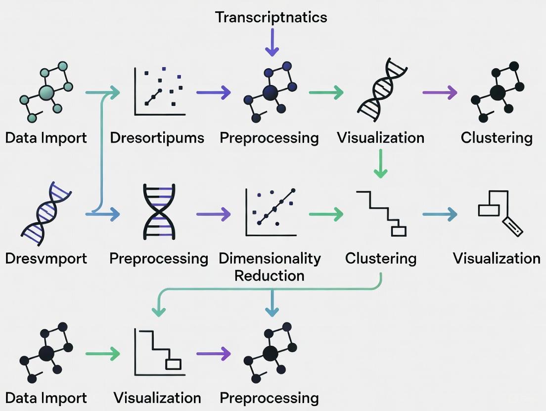
Clustering does not occur in isolation but represents a critical step in an integrated analytical pipeline. The standard workflow begins with raw data processing and quality control to remove damaged cells, dying cells, and doublets (multiple cells mistakenly identified as one) [10]. Following quality control, data normalization addresses technical variations between cells, enabling meaningful biological comparisons [13]. Feature selection then identifies highly variable genes that drive cell-to-cell heterogeneity, reducing noise and computational complexity [10] [13]. Dimensionality reduction techniques, particularly principal component analysis, transform the high-dimensional gene expression data into a lower-dimensional space that preserves essential biological signals [14]. Finally, clustering algorithms group cells based on their proximity in this reduced space, revealing distinct cell populations [6].

The following diagram illustrates the logical relationships and sequential dependencies between these key analytical steps:

Algorithmic Approaches to Clustering

Clustering algorithms for scRNA-seq data can be broadly categorized into three computational paradigms, each with distinct mechanisms and advantages:

• Classical Machine Learning Methods: These include algorithms like SC3, CIDR, and TSCAN that often employ k-means, hierarchical clustering, or model-based approaches. They typically operate on dimension-reduced data and are valued for their interpretability [6].

• Community Detection Methods: Algorithms such as Leiden and Louvain leverage graph theory by constructing cell-to-cell similarity graphs and identifying densely connected communities within these graphs. These methods are particularly efficient for large-scale datasets [6].

• Deep Learning Methods: Modern approaches including scDCC, scAIDE, and scDeepCluster use neural networks to learn non-linear representations that are optimized for clustering performance. These methods can capture complex biological relationships but require greater computational resources [6].

Benchmarking Clustering Performance

Comparative Algorithm Performance

A comprehensive 2025 benchmarking study evaluated 28 clustering algorithms across 10 paired transcriptomic and proteomic datasets using multiple performance metrics, including Adjusted Rand Index (ARI), Normalized Mutual Information (NMI), clustering accuracy, purity, memory usage, and running time [6]. The table below summarizes the top-performing methods based on this systematic evaluation:

Table 1: Top-performing single-cell clustering algorithms across transcriptomic and proteomic data

Algorithm	Class	Overall Ranking (Transcriptomics)	Overall Ranking (Proteomics)	Key Strengths
scAIDE	Deep Learning	2nd	1st	Top performance across modalities
scDCC	Deep Learning	1st	2nd	Excellent performance, memory efficient
FlowSOM	Classical ML	3rd	3rd	Robustness, fast processing
PARC	Community Detection	5th	N/R	Strong in transcriptomics
CarDEC	Deep Learning	4th	N/R	Strong in transcriptomics

Practical Considerations for Method Selection

Algorithm selection should be guided by specific experimental needs and constraints. For researchers prioritizing clustering accuracy across both transcriptomic and proteomic data, scAIDE, scDCC, and FlowSOM consistently deliver top-tier performance [6]. When computational efficiency is paramount, TSCAN, SHARP, and MarkovHC offer excellent time efficiency, while scDCC and scDeepCluster provide memory-efficient operation [6]. Community detection methods like Leiden and Louvain present a balanced option when seeking a compromise between performance and computational demands [6]. The choice of clustering resolution should align with biological questions - broader resolution may suffice for identifying major cell types, while finer resolution enables discovery of subtle cell states [6].

Experimental Protocol for scRNA-seq Clustering

Standardized Clustering Workflow

The following protocol provides a step-by-step methodology for clustering scRNA-seq data using the Seurat framework, a widely adopted analysis toolkit:

• Data Normalization: Normalize raw count data using the SCTransform() function, regressing out confounding variables such as mitochondrial content percentage and total read counts [14].

• Feature Selection: Identify highly variable genes that exhibit strong cell-to-cell variation, typically using the FindVariableFeatures() function in Seurat.

• Dimensionality Reduction: Perform principal component analysis (PCA) using the RunPCA() function. Determine the number of informative principal components to retain for downstream analysis by examining the elbow plot generated with ElbowPlot() [14].

• Batch Effect Correction: For multi-sample datasets, integrate batches using the Harmony package with the RunHarmony() function to remove technical batch effects while preserving biological variation [14].

• Cell Clustering: Construct a shared nearest neighbor graph using FindNeighbors() followed by community detection clustering with FindClusters() across a range of resolution parameters [14].

• Quality Assessment: Identify and remove low-quality clusters characterized by high mitochondrial content using VlnPlot() to visualize QC metrics across clusters. Repeat clustering iteratively until no such clusters remain [14].

• Visualization: Generate two-dimensional embeddings using Uniform Manifold Approximation and Projection (UMAP) with the RunUMAP() function for exploratory data visualization [14].

• Cluster Annotation: Perform differential expression analysis between clusters using FindMarkers() or FindConservedMarkers() to identify marker genes for cell type identification [14].

The following workflow diagram maps this procedural sequence from data input to biological interpretation:

Research Reagent Solutions

Table 2: Essential computational tools and their functions in scRNA-seq clustering analysis

Tool/Resource	Function	Application Context
Seurat	Comprehensive scRNA-seq analysis	Primary framework for clustering and visualization
Harmony	Batch effect correction	Multi-sample dataset integration
SCTransform	Normalization and variance stabilization	Data preprocessing
scAIDE	Deep learning clustering	High-performance cell type identification
scDCC	Deep learning clustering	Memory-efficient analysis of large datasets
FlowSOM	Classical machine learning clustering	Robust clustering across modalities
10X Genomics Cell Ranger	Raw data processing	UMI count matrix generation from fastq files

Advanced Applications and Integrative Approaches

Multi-Omics Integration for Enhanced Cell Identity Mapping

Clustering approaches are increasingly being extended to multimodal single-cell data, integrating transcriptomics with simultaneous measurements of surface protein expression (CITE-seq), chromatin accessibility (scATAC-seq), and other molecular features [6] [15]. Such integration provides a more comprehensive definition of cellular identity beyond transcriptomics alone. For clustering multi-omics data, specialized integration methods such as moETM, sciPENN, and totalVI create shared representations that combine information across modalities [6]. The emerging framework HALO advances this further by modeling causal relationships between chromatin accessibility and gene expression, decomposing these relationships into coupled (dependent changes) and decoupled (independent changes) components to better understand regulatory dynamics [15].

Clinical and Translational Applications

In Alzheimer's disease research, clustering of snRNA-seq data has revealed cell-type-specific molecular changes in neurodegenerative brains, identifying vulnerable neuronal populations and activated glial subpopulations contributing to disease pathology [16]. In oncology, clustering analyses have uncovered intratumoral heterogeneity, therapy-resistant cell subpopulations, and the cellular ecosystem of the tumor microenvironment [10] [11]. For drug discovery, clustering enables the identification of novel cell states that may represent therapeutic targets and facilitates drug screening using patient-derived organoid models [10] [11].

Clustering remains the cornerstone computational method for extracting biological meaning from scRNA-seq data, transforming high-dimensional gene expression measurements into interpretable cellular taxonomies. As single-cell technologies continue to evolve toward multi-omic assays and increased throughput, clustering methodologies must similarly advance to leverage these rich data sources. The integration of causal modeling approaches like HALO [15] with robust clustering frameworks represents the cutting edge of cell identity mapping. For biomedical researchers, careful selection of clustering algorithms based on benchmarking studies [6] and implementation of standardized workflows [14] will ensure biologically meaningful results that accelerate both basic research and translational applications across diverse fields from neurobiology to oncology.

How Hierarchical Clustering Complements Other Exploratory Methods like PCA

In transcriptomics research, exploratory data analysis is a critical first step for extracting meaningful biological insights from high-dimensional datasets. Among the most widely used unsupervised methods, Principal Component Analysis (PCA) and hierarchical clustering each offer distinct advantages and, when used together, provide a more comprehensive understanding of cellular heterogeneity and gene expression patterns [17]. PCA serves as a powerful dimensionality reduction technique, creating a low-dimensional representation of samples that optimally preserves the variance within the original dataset [17]. In contrast, hierarchical clustering builds a tree-like structure that successively groups similar objects based on their expression profiles, serving both visualization and partitioning functions [17] [2]. This application note examines the complementary relationship between these methods within the context of transcriptomics data analysis, providing detailed protocols for their implementation and integration.

Theoretical Foundation and Comparative Analysis

Core Principles of PCA and Hierarchical Clustering

PCA reduces data dimensionality by identifying orthogonal principal components (PCs) that capture maximum variance, with the first component (PC1) representing the largest variance source, followed by PC2, and so on [18]. The resulting low-dimensional projection filters out weak signals and noise, potentially revealing cleaner patterns than raw data visualizations [17]. PCA also provides synchronized sample and variable representations, allowing researchers to identify variables characteristic of specific sample groups [17].

Hierarchical clustering creates a hierarchical nested clustering tree through iterative pairing of the most similar objects [2]. The algorithm employs a bottom-up (agglomerative) approach, calculating similarity between all sample pairs using measures like Euclidean distance, then successively merging the closest pairs into clusters until all objects unite in a single tree [17] [2]. The resulting dendrogram provides intuitive visualization of relationships between samples or genes, with heatmaps enabling simultaneous examination of expression patterns across the entire dataset [17].

Comparative Strengths and Limitations

Table 1: Comparative analysis of PCA and hierarchical clustering characteristics

Characteristic	PCA	Hierarchical Clustering
Primary Function	Dimensionality reduction and variance capture	Grouping and tree-structure visualization
Data Processing	Filters out low-variance components	Uses all data without filtering
Output	Low-dimensional sample projection	Dendrogram with associated heatmap
Group Definition	Reveals natural groupings through variance separation	Always creates clusters, even with weak signal
Noise Handling	Discards low-variance components (often noise)	Displays all data, including potential noise
Interpretation	Sample positions indicate similarity	Branch lengths indicate similarity degrees

The most significant distinction lies in their fundamental approaches: PCA prioritizes variance representation while hierarchical clustering focuses on similarity-based grouping [17]. This difference makes them naturally complementary rather than competitive. In practice, when strong biological signals exist (e.g., distinct cell subtypes), both methods typically reveal concordant patterns, as demonstrated in studies of acute lymphoblastic leukemia where both approaches clearly separated different patient subtypes [17].

Integrated Analytical Protocol for Transcriptomics Data

Preprocessing and Quality Control

Sample Preparation and RNA Sequencing

• Isolate high-quality RNA (RIN > 7.0) from samples using appropriate kits (e.g., PicoPure RNA Isolation Kit) [18]
• Prepare cDNA libraries using poly(A) selection and library preparation kits (e.g., NEBNext Ultra DNA Library Prep Kit) [18]
• Sequence libraries on appropriate platforms (e.g., Illumina NextSeq 500) to obtain sufficient read depth (e.g., 8 million aligned reads per library) [18]

Data Processing and Normalization

• Demultiplex raw sequencing data (e.g., using bcl2fastq) [18]
• Align reads to reference genome (e.g., mm10 for mouse) using aligners like TopHat2 [18]
• Generate raw count matrices using tools like HTSeq [18]
• Apply appropriate normalization methods (e.g., Scran or SCNorm) to address technical variability [19]

Batch Effect Mitigation

• Control for technical variations by processing experimental and control conditions simultaneously [18]
• Minimize operator variability through standardized protocols
• Harvest samples at consistent times to control for circadian effects
• Sequence all comparison groups in the same run to minimize technical batch effects [18]

Protocol for Complementary Analysis

PCA Implementation and Interpretation

• Input Preparation: Use normalized count matrices, optionally filtering low-count genes
• Dimensionality Reduction: Apply PCA to obtain principal components using standard implementations (R: prcomp, Python: sklearn.decomposition.PCA) [19]
• Variance Assessment: Examine scree plot to determine the number of meaningful components
• Visualization: Plot samples in 2D or 3D space using the first 2-3 principal components
• Pattern Identification: Identify sample groupings and outliers in the reduced space
• Variable Examination: Analyze component loadings to identify genes driving separation

Hierarchical Clustering Implementation

• Distance Calculation: Compute pairwise distances between samples using Euclidean distance
• Linkage Method Selection: Choose appropriate linkage method (e.g., Ward's method)
• Tree Construction: Build dendrogram through iterative clustering (R: hclust, Python: scikit-learn hierarchical clustering) [19]
• Heatmap Integration: Visualize data matrix with samples ordered by dendrogram structure
• Cluster Identification: Cut dendrogram at appropriate height to define sample groups

Integrated Interpretation

• Concordance Check: Compare PCA groupings with hierarchical clustering results
• Pattern Validation: Use consistent coloring in both visualizations to identify corresponding patterns
• Marker Identification: Combine PCA loadings with heatmap patterns to identify group-specific genes
• Biological Validation: Correlate computational groupings with known biological variables

Workflow Visualization

Figure 1: Integrated analytical workflow for transcriptomics data exploration

Essential Research Reagent Solutions

Table 2: Key reagents and computational tools for transcriptomics analysis

Category	Specific Tool/Reagent	Function/Application
RNA Isolation	PicoPure RNA Isolation Kit	High-quality RNA extraction from limited samples [18]
Library Prep	NEBNext Poly(A) mRNA Magnetic Isolation Kit	mRNA enrichment for transcriptome sequencing [18]
cDNA Synthesis	NEBNext Ultra DNA Library Prep Kit	Library preparation for Illumina sequencing [18]
Alignment	TopHat2	Read alignment to reference genomes [18]
Quantification	HTSeq	Generation of raw count matrices from aligned reads [18]
Normalization	Scran	Pool-based size factors for single-cell normalization [19]
Differential Expression	edgeR	Negative binomial models for DEG identification [18]
Clustering Algorithms	Hierarchical clustering, K-means, Leiden	Sample and gene grouping approaches [19]

Advanced Applications and Method Integration

Single-Cell and Spatial Transcriptomics Extensions

The PCA and hierarchical clustering framework extends to advanced transcriptomics applications. In single-cell RNA sequencing, these methods help identify cell subpopulations and validate clustering results [6]. For spatial transcriptomics, specialized tools like BayesSpace, SpaGCN, and STAGATE incorporate spatial coordinates alongside expression values to define spatially coherent domains while maintaining the fundamental principles of expression-based clustering [20].

Multi-Omics Data Integration

Recent benchmarking studies demonstrate that clustering methods like scDCC, scAIDE, and FlowSOM perform robustly across both transcriptomic and proteomic data [6]. When analyzing integrated multi-omics data, PCA and hierarchical clustering remain valuable for initial exploration and quality assessment before applying more specialized integration algorithms.

Figure 2: Complementary strengths of PCA and hierarchical clustering

PCA and hierarchical clustering offer complementary approaches for exploratory transcriptomics analysis. PCA excels at capturing major variance components and filtering noise, while hierarchical clustering provides intuitive similarity-based groupings with detailed expression pattern visualization. Used together within a structured analytical protocol, these methods enable robust identification of biologically meaningful patterns in transcriptomics data, forming an essential foundation for subsequent hypothesis-driven research and biomarker discovery in both basic research and drug development contexts.

Single-cell RNA sequencing (scRNA-seq) has revolutionized transcriptomics by enabling the comprehensive analysis of gene expression profiles at the individual cell level, providing unprecedented insights into cellular heterogeneity in complex biological systems [11]. This technology has fundamentally transformed our ability to investigate how different cells behave at single-cell resolution, uncovering new insights into biological processes that were previously masked in bulk RNA-seq experiments [11]. The key contrast between bulk RNA-seq and scRNA-seq lies in whether each library reflects an individual cell or a cell group, driven by unique challenges including scarce transcripts in single cells, inefficient mRNA capture, losses in reverse transcription, and bias in cDNA amplification due to the minute amounts involved [11].

The applications of scRNA-seq span multiple domains including drug discovery, tumor microenvironment characterization, biomarker discovery, and microbial profiling [11]. Through scRNA-seq, researchers have gained the potential to uncover previously unknown cell types, map developmental pathways, and investigate the complexity of tumor diversity [11]. This technology is particularly valuable when addressing crucial biological inquiries related to cell heterogeneity and early embryo development, especially in cases involving a limited number of cells [11]. The ability to resolve cellular heterogeneity through clustering analysis forms the foundation for many of these applications, making hierarchical clustering approaches essential for extracting meaningful biological insights from high-dimensional scRNA-seq data.

Analytical Framework and Workflow

Core Computational Workflow

A robust analytical workflow is essential for transforming raw scRNA-seq data into biologically meaningful insights. The standard workflow encompasses multiple critical stages, beginning with quality control to identify and remove low-quality cells and data that might represent multiple cells [11]. Subsequent steps include data normalization, feature selection, dimensionality reduction, and clustering analysis—with the latter being particularly crucial for identifying distinct cell populations [11]. The clustering results then enable downstream analyses such as differential expression, which can compare average expression between cell types or conditions [21].

Specialized computational tools tailored to scRNA-seq data are essential due to the unique characteristics of this data type, which is often noisy, high-dimensional, and sparsely populated [11]. The selection of appropriate analytical methods is further complicated by the explosion of single-cell analysis tools, making it challenging for researchers to choose the right tool for their specific dataset [11]. This challenge extends to clustering algorithms, where methodological selection significantly impacts the reliability and interpretation of results.

Table 1: Key Stages in scRNA-seq Data Analysis

Analysis Stage	Purpose	Common Tools/Approaches
Quality Control	Filter low-quality cells and multiplets	FastQC, Trimmomatic
Normalization	Account for technical variability	SCTransform, LogNormalize
Feature Selection	Identify biologically relevant genes	HVG selection
Dimensionality Reduction	Visualize and compress data	PCA, UMAP, t-SNE
Clustering	Identify distinct cell populations	Leiden, Louvain, scDCC
Differential Expression	Find marker genes between groups	MAST, DESeq2, edgeR

Workflow Visualization

Application 1: Resolving Cellular Heterogeneity

Experimental Protocol for Cell Type Identification

Objective: To identify distinct cell populations within a complex tissue sample using scRNA-seq clustering analysis.

Sample Preparation and Single-Cell Isolation:

• Extract viable single cells from the tissue of interest using appropriate dissociation protocols [11].
• For tissues where dissociation is challenging, consider single-nuclei RNA-seq (snRNA-seq) as an alternative [11].
• Isolate individual cells using fluorescence-activated cell sorting (FACS) or droplet-based microfluidics depending on throughput requirements [11].
• Perform cell lysis to release RNA molecules and capture polyadenylated mRNA using poly[T]-primers while minimizing ribosomal RNA capture [11].

Library Preparation and Sequencing:

• Select appropriate scRNA-seq protocol based on research goals (e.g., full-length transcript protocols like Smart-Seq2 for isoform analysis, or 3'-end counting protocols like Drop-Seq for high-throughput applications) [11].
• Incorporate Unique Molecular Identifiers (UMIs) to correct for amplification bias and enable accurate transcript quantification [11].
• Prepare sequencing libraries following protocol-specific guidelines, with particular attention to amplification method (PCR-based or in vitro transcription) [11].
• Sequence libraries using an Illumina platform with sufficient depth to capture the transcriptional diversity of individual cells.

Computational Analysis:

• Perform quality control using tools like FastQC and Trimmomatic to remove low-quality reads and adapter sequences [22].
• Align reads to the reference genome using dedicated scRNA-seq alignment tools for efficient resource utilization [11].
• Generate a gene expression matrix with cells as columns and genes as rows, incorporating UMI counts [11].
• Apply normalization methods to correct for technical variability between cells [22].
• Identify highly variable genes to focus on biologically relevant features [6].
• Perform dimensionality reduction using PCA followed by visualization with UMAP or t-SNE [6].
• Execute clustering analysis using graph-based methods (Leiden, Louvain) or other advanced algorithms [6] [23].

Benchmarking Clustering Performance

The selection of appropriate clustering algorithms is critical for accurate cell type identification. Recent benchmarking studies have evaluated 28 computational algorithms on 10 paired transcriptomic and proteomic datasets, assessing performance across various metrics including clustering accuracy, peak memory usage, and running time [6]. These studies reveal that different algorithms demonstrate varying strengths depending on the data modality and analytical requirements.

Table 2: Performance of Top scRNA-seq Clustering Algorithms

Algorithm	Type	ARI Score	NMI Score	Computational Efficiency	Best Use Cases
scDCC	Deep learning	High	High	Moderate	Top performance across omics
scAIDE	Deep learning	High	High	Moderate	Proteomic data
FlowSOM	Machine learning	High	High	High	Large datasets, robustness
PARC	Community detection	Moderate	Moderate	High	Transcriptomic data
Leiden	Graph-based	Moderate	Moderate	High	Standard scRNA-seq analysis
Louvain	Graph-based	Moderate	Moderate	High	General purpose clustering

The table above summarizes the performance characteristics of leading clustering algorithms, with scDCC, scAIDE, and FlowSOM demonstrating the strongest performance across both transcriptomic and proteomic data [6]. These algorithms excel in key metrics including Adjusted Rand Index (ARI) and Normalized Mutual Information (NMI), which quantify clustering quality by comparing predicted and ground truth labels [6].

Enhancing Clustering Reliability

A significant challenge in clustering analysis is the inconsistency that arises from stochastic processes in clustering algorithms [23]. The single-cell Inconsistency Clustering Estimator (scICE) was developed to address this limitation by evaluating clustering consistency and providing consistent clustering results [23]. This approach achieves up to a 30-fold improvement in speed compared to conventional consensus clustering-based methods such as multiK and chooseR, making it practical for large datasets exceeding 10,000 cells [23].

The scICE framework employs the inconsistency coefficient (IC) to evaluate label consistency without requiring hyperparameters or computationally expensive consensus matrices [23]. When applied to real and simulated scRNA-seq datasets, scICE revealed that only approximately 30% of clustering numbers between 1 and 20 were consistent, enabling researchers to focus on a narrower set of reliable candidate clusters [23]. This approach significantly enhances the efficiency and robustness of cellular heterogeneity analysis.

Application 2: Uncovering Developmental Trajectories

Experimental Protocol for Trajectory Inference

Objective: To reconstruct cellular differentiation pathways and developmental processes from scRNA-seq data.

Experimental Design:

• Collect samples across multiple time points during the developmental process of interest.
• Ensure sufficient cell coverage at each time point to capture rare transitional states.
• Process samples individually with appropriate sample multiplexing to minimize batch effects.
• Include biological replicates to ensure statistical robustness of inferred trajectories.

Computational Analysis for Trajectory Inference:

• Perform standard scRNA-seq processing and clustering as described in Section 3.1.
• Identify potential branching points and transitional cell states through careful examination of clustering results in low-dimensional embeddings.
• Apply trajectory inference algorithms (e.g., Monocle3, Slingshot) to reconstruct developmental paths.
• Order cells along pseudotime trajectories to model progression through developmental stages.
• Identify genes with dynamic expression patterns along the trajectories.
• Validate key transitional states using marker gene expression and functional enrichment analysis.

Advanced Analytical Approaches

Beyond standard trajectory inference, several advanced approaches enhance the resolution of developmental analyses:

Differential Detection Analysis: While traditional differential expression tools compare average expression between cell types, differential detection workflows infer differences in the average fraction of cells in which expression is detected [21]. This approach provides complementary information to standard differential expression analysis, both in terms of individual genes reported and their functional interpretation [21]. Through simulations and case studies, joint analyses of differential expression and differential detection have demonstrated enhanced capability to uncover biologically relevant patterns in developmental processes [21].

Spatial Transcriptomics Integration: Spatial transcriptomics technologies significantly advance trajectory analysis by quantifying gene expression within tissue sections while preserving crucial spatial context information [24]. By integrating multiple tissue slices, researchers can achieve a comprehensive 3D reconstruction of developing tissues, preserving spatial relationships that cannot be captured in isolated 2D slices [24]. This holistic perspective is critical for studying complex tissue architectures and developmental processes, offering insights into cellular organization, interactions, and spatial gradients of gene expression [24].

Trajectory Analysis Visualization

The Scientist's Toolkit

Research Reagent Solutions

Table 3: Essential Reagents and Materials for scRNA-seq Applications

Reagent/Material	Function	Example Protocols	Considerations
Poly[T] Primers	Capture polyadenylated mRNA	All scRNA-seq protocols	Minimizes ribosomal RNA capture
Unique Molecular Identifiers (UMIs)	Correct for amplification bias	Drop-Seq, inDrop, 10X Genomics	Enables accurate transcript counting
Hydrogel Beads	Encapsulate individual cells	inDrop	Low cost per cell
Microfluidic Chips	Single-cell isolation	Drop-Seq, 10X Genomics	High-throughput processing
Cell Lysis Buffers	Release RNA content	All protocols	Maintains RNA integrity
Reverse Transcription Mix	cDNA synthesis	Smart-Seq2, CEL-Seq2	Protocol-specific optimization
PCR Amplification Mix	cDNA amplification	Most protocols	Can introduce bias if not optimized
In Vitro Transcription Mix	RNA amplification	CEL-Seq2, inDrop	Linear amplification reduces bias
8-Hydroxy Amoxapine-d8	8-Hydroxy Amoxapine-d8, MF:C17H16ClN3O2, MW:337.8 g/mol	Chemical Reagent	Bench Chemicals
4-(4-Chlorophenyl)cyclohexanol-d5	4-(4-Chlorophenyl)cyclohexanol-d5, CAS:1189961-66-7, MF:C12H15ClO, MW:215.73 g/mol	Chemical Reagent	Bench Chemicals

The selection of computational tools is as critical as wet laboratory reagents for successful scRNA-seq applications. Recent benchmarking studies provide guidance for tool selection across various analytical scenarios [6] [23]. For clustering analysis, methods such as scDCC, scAIDE, and FlowSOM demonstrate strong performance across different data modalities, while tools like scICE enhance reliability by evaluating clustering consistency [6] [23].

For differential expression analysis, a comprehensive benchmarking of 288 pipelines revealed that careful selection of analytical tools based on the specific biological context provides more accurate biological insights compared to default software configurations [22]. This highlights the importance of tailored analytical strategies rather than indiscriminate tool selection for achieving high-quality results [22].

Single-cell RNA sequencing has fundamentally transformed our ability to investigate cellular heterogeneity and developmental trajectories at unprecedented resolution. The applications outlined in this document—from resolving complex cell populations to reconstructing developmental pathways—demonstrate the power of this technology to uncover novel biological insights. However, realizing this potential requires careful experimental design, appropriate protocol selection, and robust computational analysis.

The integration of advanced computational methods, including reliable clustering algorithms and trajectory inference approaches, enables researchers to extract meaningful biological knowledge from high-dimensional scRNA-seq data. Furthermore, emerging technologies such as spatial transcriptomics and multi-omics integration promise to further enhance our understanding of biological systems in their native context. As the field continues to evolve, the standardized protocols and benchmarking data presented here provide a foundation for rigorous and reproducible single-cell research, ultimately advancing our knowledge of cellular behavior in health and disease.

Core Concepts and Workflow

Hierarchical clustering is an unsupervised machine learning method used to build a hierarchy of clusters, revealing underlying structures within complex datasets like those in transcriptomics research [25] [26]. Its application allows researchers to explore gene expression patterns without a priori assumptions, grouping genes or samples based on similarity [1].

There are two primary algorithmic strategies, as outlined in Table 1 [25] [26]:

Table 1: Hierarchical Clustering Algorithm Types

Algorithm Type	Approach	Description	Best Use Cases
Agglomerative	Bottom-Up	Begins with each data point as its own cluster and iteratively merges the most similar pairs until one cluster remains. [25]	Common default method; suitable for identifying smaller, tighter clusters. [25] [26]
Divisive	Top-Down	Starts with all data points in a single cluster and recursively splits them into smaller clusters. [25]	Identifying large, distinct clusters first; can be more accurate but computationally expensive. [25] [26]

The results are universally presented in a dendrogram, a tree-like diagram that visualizes the sequence of cluster merges (or splits) and the similarity (distance) at which each merge occurred [25] [26]. The height at which two clusters are joined represents the distance between them, allowing researchers to understand the nested cluster relationships intuitively.

Figure 1: A generalized workflow for performing hierarchical clustering on transcriptomics data, from raw data to biological interpretation.

Distance Metrics

The choice of distance metric fundamentally defines the concept of "similarity" between two data points, such as genes or samples. For transcriptomics data, where the pattern of expression across conditions is often more critical than absolute expression levels, correlation-based distances are widely used [27].

Table 2: Common Distance Metrics for Transcriptomics Data

Distance Metric	Formula	Application in Transcriptomics
Euclidean	( d(x, y) = \sqrt{\sum{i=1}^n (xi - y_i)^2} )	Measures geometric ("as-the-crow-flies") distance. Sensitive to absolute expression levels. [27]
Correlation	( d(x, y) = 1 - r ) (Pearson/Spearman)	Ideal for clustering genes based on co-expression patterns, as it is invariant to shifts in baseline expression. [27]
Absolute Correlation	( d(x, y) = 1 - |r| )	Clusters genes with strong positive OR negative correlations (e.g., regulatory relationships). [27]
Manhattan	( d(x, y) = \sum{i=1}^n |xi - y_i| )	Less sensitive to outliers than Euclidean distance. [27]

A critical step in transcriptomics analysis is data pre-processing. Centering (subtracting the mean) and scaling (dividing by the standard deviation to create z-scores) transform the data. Using Euclidean distance on z-scores is equivalent to using correlation distance on the original data, which focuses the analysis purely on expression patterns [27].

Linkage Methods

The linkage criterion determines how the distance between clusters (as opposed to individual points) is calculated, profoundly influencing the shape and compactness of the resulting clusters [25] [27].

Table 3: Comparison of Common Linkage Methods

Linkage Method	Formula	Cluster Shape Tendency	Pros and Cons
Single	( D(A,B) = \min{d(a,b) | a \in A, b \in B} )	String-like, elongated	Pro: Can handle non-elliptical shapes. Con: Sensitive to noise and outliers; "chaining effect." [26] [27]
Complete	( D(A,B) = \max{d(a,b) | a \in A, b \in B} )	Ball-like, compact	Pro: Less sensitive to noise; produces tight, spherical clusters. Con: Can be biased by large clusters. [25] [26] [27]
Average (UPGMA)	( D(A,B) = \frac{1}{|A|\cdot|B|}\sum{a \in A}\sum{b \in B} d(a,b) )	Ball-like, compact	A balanced compromise between Single and Complete linkage. [25] [27]
Ward	( D(A,B) = \frac{|A|\cdot|B|}{|A \cup B|} || \muA - \muB ||^2 )	Ball-like, compact	Pro: Minimizes within-cluster variance; creates clusters of similar size. Less affected by outliers. [26]

For gene expression data, a combination of correlation distance and complete linkage clustering is frequently employed and often provides biologically meaningful results [27].

Protocol for Hierarchical Clustering of Transcriptomics Data

Pre-processing and Distance Calculation

• Data Normalization: Normalize raw read counts (e.g., from RNA-seq) to account for library size and other technical variations. Common methods include TPM (Transcripts Per Million), FPKM (Fragments Per Kilobase Million), or using tools like DESeq2 or edgeR.
• Transformation: Apply a logarithmic transformation, typically ( \log2(\text{expression} + \text{pseudocount}) ), to stabilize variance and make the data more symmetric. A pseudocount (e.g., 0.25, 1) is added to handle zero values [27].
• Filtering: Filter out genes with very low expression or minimal variance across samples to reduce noise.
• Distance Matrix Computation: Calculate the pairwise distance matrix between all items (genes or samples). For clustering genes by expression pattern, correlation distance is highly recommended [1] [27].

Agglomerative Clustering Execution

• Input: Begin with a dissimilarity matrix and 'n' clusters, each containing a single data point [25] [26].
• Linkage Criterion: Select a linkage method (see Table 3). Complete linkage is a robust default for transcriptomics [27].
• Iterative Merging: Identify the two clusters with the smallest distance according to the linkage criterion. Merge these two clusters into a new, larger cluster [25] [26].
• Matrix Update: Update the distance matrix to reflect the distances between the new cluster and all remaining clusters using the Lance-Williams recursive formula [26].
• Repetition: Repeat steps 3 and 4 until all data points are contained within a single root cluster [25] [26].

Interpreting the Dendrogram and Defining Clusters

The final dendrogram provides a complete history of the merging process. To obtain specific clusters for downstream analysis, the dendrogram must be "cut."

Figure 2: Interpreting a dendrogram. Cutting at different heights (H1, H2) yields different numbers of clusters, allowing researchers to choose the most biologically relevant granularity.

• Determine the Cut Height: The number of clusters is determined by the number of vertical lines intersected by a horizontal "cut" line across the dendrogram. The height of this line corresponds to the dissimilarity at which clusters are defined [26].
• Selecting the Number of Clusters (k):
  • Domain Knowledge: Use biological context to guide a sensible number of clusters (e.g., expected cell types or pathways).
  • The Elbow Method: Plot the within-cluster sum of squares against the number of clusters. The "elbow" point, where the sum of squares stops decreasing sharply, can indicate a good value for k [26].
  • Dendrogram Inspection: Look for the highest levels of the tree where branches are long, indicating a clear separation between clusters. The optimal number of clusters is often where the vertical lines in the dendrogram have the most considerable space to move up and down without crossing another horizontal merge line [26].

The Scientist's Toolkit

Table 4: Essential Research Reagent Solutions for Transcriptomics Clustering

Item	Function in Analysis
RNA-seq Library Prep Kit	Generates the sequencing libraries from RNA samples. Essential for producing the raw count data used in clustering.
Normalization Software (e.g., DESeq2, edgeR)	Performs statistical normalization on raw count data to remove technical biases, a critical pre-processing step before clustering.
Statistical Software (R/Python)	Provides the computational environment and libraries (e.g., R stats, hclust, factoextra) to perform distance calculation, clustering, and visualization.
Visualization Package (e.g., ggplot2, pheatmap)	Enables the creation of publication-quality dendrograms and heatmaps to visualize clustering results and communicate findings.
N-Demethyl Lincomycin Hydrochloride	N-Demethyl Lincomycin Hydrochloride, CAS:14600-41-0, MF:C17H33ClN2O6S, MW:429.0 g/mol
2-Ethyl-6-methylaniline-d13	2-Ethyl-6-methylaniline-d13, MF:C9H13N, MW:148.29 g/mol

Step-by-Step Implementation: From Data Preparation to Dendrogram Interpretation

In transcriptomics research, hierarchical clustering is a fundamental technique for exploring gene expression patterns and identifying novel biological relationships. The reliability of its output is profoundly dependent on the quality of the input data, making optimal data preprocessing not merely a preliminary step but the foundation of robust analysis. This document details applied protocols for two critical preprocessing steps—data normalization and highly variable gene (HVG) selection—specifically framed within the context of preparing data for hierarchical clustering. Proper normalization removes technical noise, enabling valid comparisons across samples, while effective HVG selection reduces dimensionality to highlight biologically meaningful signals. Together, these steps ensure that hierarchical clustering reveals true underlying biological structure rather than technical artifacts or random noise [28] [29].

Normalization Strategies

Normalization adjusts raw gene expression data to eliminate systematic technical variations, such as those arising from differences in sequencing depth, library preparation, or platform-specific effects. This is a prerequisite for any downstream comparative analysis, including hierarchical clustering, as it ensures that the distances between data points reflect biological differences rather than technical bias [28].

Normalization Methods for Transcriptomic Data

Various normalization methods are employed in transcriptomic data analysis. The choice of method depends on the data type (e.g., microarray vs. RNA-seq) and the specific goals of the analysis, such as cross-platform compatibility.

Table 1: Comparison of Common Normalization Methods

Method Name	Underlying Principle	Best For	Key Advantages	Key Limitations
LOG_QN [28]	Applies a log transformation followed by quantile normalization.	Cross-platform classification (e.g., Microarray & RNA-seq).	Effective for machine learning model transfer across platforms.	Performance may vary with dataset characteristics.
LOG_QNZ [28]	LOG_QN with an added z-score standardization.	Cross-platform classification where feature scaling is critical.	Improves model performance by standardizing feature scales.	Adds complexity to the data pipeline.
NDEG-Based Normalization [28]	Uses non-differentially expressed genes (NDEGs) as a stable reference set.	Scenarios requiring a robust, biologically-informed reference set.	Leverages biologically stable genes; improves cross-platform performance.	Relies on accurate identification of NDEGs.
Standard Z-Score	Standardizes data to a mean of zero and standard deviation of one.	General-purpose normalization for many downstream analyses.	Simple, intuitive, and widely applicable.	Can be sensitive to outliers.
Quantile Normalization	Forces the distribution of expression values to be identical across samples.	Making sample distributions comparable.	Creates uniform distributions across samples.	Assumes most genes are not differentially expressed.

Protocol: NDEG-Based Normalization for Cross-Platform Robustness

This protocol outlines a robust normalization strategy using NDEGs, which is particularly useful when building models on one transcriptomics platform (e.g., RNA-seq) and applying them to another (e.g., microarray) [28].

Experimental Reagents and Equipment

• Raw Gene Expression Matrix: A count matrix (for RNA-seq) or intensity matrix (for microarray) where rows represent genes and columns represent samples.
• Computational Environment: Python (version 3.11.9 or later) with scientific computing libraries (NumPy, Pandas, Scikit-learn).
• Sample Annotation File: A file containing the molecular subtype or experimental group for each sample.

Step-by-Step Procedure

• Data Cleaning: Load the raw gene expression matrix and sample annotation file. Filter the dataset to retain only samples with available class labels (e.g., molecular subtypes). Subsequently, remove any genes that contain missing values to create a complete matrix of shared genes across all samples [28].
• Non-Differentially Expressed Gene (NDEG) Selection: a. Perform ANOVA: For each gene in the cleaned matrix, perform a one-way Analysis of Variance (ANOVA) using the sample class labels as groups. The goal is to test the null hypothesis that the gene's expression does not differ between classes. b. Calculate F-value: Compute the F-statistic for each gene using the formula: F = MSB / MSW = [Σn_i(Ȳ_i - Ȳ)^2 / (k-1)] / [ΣΣ(Y_ij - Ȳ_i)^2 / (N-k)] where MSB is the mean square between groups, MSW is the mean square within groups, k is the number of groups, N is the total sample size, n_i is the sample size per group, Ȳ_i is the group mean, and Ȳ is the overall mean [28]. c. Select NDEGs: Genes with a high p-value (e.g., p > 0.85) from the ANOVA test fail to reject the null hypothesis, indicating their expression is stable across classes. These genes are selected as the NDEG set for normalization [28].
• Apply Normalization: a. Subset Data: Create a new matrix containing only the expression values of the selected NDEGs. b. Perform LOGQN Normalization: i. Log Transformation: Apply a log2 transformation to the NDEG expression matrix to reduce the effect of extreme values. ii. Quantile Normalization: Normalize the log-transformed data across samples so that the distribution of expression values is identical for each sample [28]. c. (Optional) Perform LOGQNZ Normalization: For an additional standardization step, apply a z-score transformation to the LOG_QN normalized data, standardizing each gene to have a mean of 0 and a standard deviation of 1 [28].

Selection of Highly Variable Genes

Following normalization, selecting HVGs is a critical dimensionality reduction step. This process filters out genes that exhibit little variation across cells or samples, which likely represent uninteresting technical noise or biological "housekeeping" functions. By focusing on the most variable genes, the analysis highlights features that are most likely to be biologically informative, such as those driving cellular heterogeneity. This leads to a cleaner and more interpretable distance matrix for hierarchical clustering, ultimately revealing more distinct and biologically relevant clusters [29] [30].

HVG Selection Methods

Multiple computational methods have been developed to identify HVGs, each with different underlying assumptions and strengths.

Table 2: Comparison of Highly Variable Gene (HVG) Selection Methods

Method Name	Underlying Principle	Key Feature	Advantages	Disadvantages/Limitations
GLP [29]	Optimized LOESS regression on the relationship between a gene's positive ratio (f) and its mean expression (λ).	Uses Bayesian Information Criterion for automatic bandwidth selection to avoid overfitting.	Robust to sparsity and dropout noise; enhances downstream clustering.	A newer method, less integrated into standard pipelines.
VST [29] [30]	Fits a smooth curve to the mean-variance relationship and standardizes expression based on this model.	Part of the widely used Seurat package.	Established, widely-used method.	Can be influenced by high sparsity.
SCTransform [29] [30]	Uses Pearson residuals from a regularized negative binomial generalized linear model.	Models single-cell data specifically, accounting for over-dispersion.	Integrated into Seurat workflow; models count data well.	Computationally more intensive than VST.
M3Drop [29]	Fits a Michaelis-Menten function to model the relationship between mean expression and dropout rate.	Leverages dropout information, common in single-cell data.	Useful for capturing genes with bimodal expression.	Relies on characteristics of dropout noise.

Protocol: HVG Selection using the GLP Algorithm

The GLP (LOESS with Positive Ratio) algorithm is a robust feature selection method that precisely captures the non-linear relationship between a gene's average expression level and its positive ratio, making it particularly effective for sparse data like single-cell RNA-seq [29].

Experimental Reagents and Equipment

• Normalized Expression Matrix: A pre-processed and normalized gene expression matrix (from Section 2).
• Computational Environment: R or Python with necessary statistical libraries and the GLP implementation.

Step-by-Step Procedure

• Calculate Metrics: a. Mean Expression (λ): For each gene j, calculate its mean expression level across all samples (or cells) c using the formula: λ_j = (1/c) * Σ X_ij where X_ij is the expression of gene j in sample i [29]. b. Positive Ratio (f): For each gene j, calculate the proportion of samples (or cells) in which it is detected. Formally: f_j = (1/c) * Σ min(1, X_ij) [29].
• Filter Low-Prevalence Genes: Remove any genes that are detected in fewer than a minimum number of samples (e.g., 3 cells in scRNA-seq data) to avoid unreliable metrics [29].
• Determine Optimal Smoothing Parameter: a. The LOESS regression requires a smoothing parameter ⍺. The GLP algorithm automatically determines the optimal ⍺ by testing a range of values (e.g., from 0.01 to 0.1) [29]. b. For each candidate ⍺, perform a LOESS regression of λ (dependent variable) on f (independent variable). Calculate the Bayesian Information Criterion (BIC) for each model: BIC = c * ln(RSS/c) + k * ln(c), where RSS is the residual sum of squares, c is the number of observations (genes), and k is the model degrees of freedom [29]. c. Select the ⍺ value that yields the lowest BIC, indicating the best fit without overfitting.
• Perform Two-Step LOESS Regression: a. First Fit: Using the optimal ⍺, fit a LOESS model to the (f, λ) data for all genes. Apply Tukey's biweight robust method to identify genes that are outliers from the fitted curve [29]. b. Second Fit: Assign zero weight to the outlier genes identified in the first step and re-fit the LOESS model. This minimizes the influence of true biological outliers, leading to a more accurate baseline [29].
• Select Highly Variable Genes: Genes whose actual mean expression level (λ) is significantly greater than the value predicted (λ_pred) by the final LOESS model are considered highly variable. Select the top N genes with the largest positive residuals (λ - λ_pred) for downstream hierarchical clustering [29].

Integrated Workflow for Hierarchical Clustering

The following diagram illustrates the logical sequence of data preprocessing and its direct connection to hierarchical clustering, integrating the protocols described in this document.

Preprocessing Workflow for Clustering

The Scientist's Toolkit

This section details the essential software and computational tools required to implement the protocols described in this document.

Table 3: Essential Research Reagent Solutions for Computational Analysis

Tool/Resource	Type	Primary Function in Preprocessing	Key Application
Python (v3.11+)	Programming Language	Provides the core environment for implementing custom normalization and HVG selection scripts, such as the NDEG-based and GLP protocols.	Flexible, code-based analysis pipelines [28].
R	Programming Language	Ecosystem for statistical computing; hosts implementations of many popular HVG methods (e.g., in Seurat, SCTransform) and normalization techniques.	Statistical analysis and visualization [31] [30].
Seurat	R/Python Package	A comprehensive toolkit for single-cell analysis, offering integrated functions for normalization (e.g., LogNormalize) and HVG selection (e.g., VST, SCTransform) [29] [30].	Standardized single-cell RNA-seq analysis.
Scanpy	Python Package	A scalable toolkit for single-cell data analysis, analogous to Seurat, providing similar normalization and HVG selection capabilities within the Python ecosystem.	Standardized single-cell RNA-seq analysis.
TCGA BRCA Dataset	Reference Data	A publicly available dataset containing matched microarray and RNA-seq data, used for benchmarking and validating cross-platform normalization methods [28].	Method validation and benchmarking.
5'-Cholesteryl-TEG PhosphoraMidite	5'-Cholesteryl-TEG Phosphoramidite|Oligo Synthesis Reagent	Research-grade 5'-Cholesteryl-TEG Phosphoramidite for enhancing oligonucleotide cellular uptake. For Research Use Only. Not for human or veterinary use.	Bench Chemicals
Bis(4-Methyl-2-pentyl) Phthalate-d4	Bis(4-Methyl-2-pentyl) Phthalate-d4, CAS:1398066-13-1, MF:C20H30O4, MW:338.5 g/mol	Chemical Reagent	Bench Chemicals

In transcriptomics research, distance metrics are mathematical functions that quantify the dissimilarity between gene expression profiles. The choice of metric fundamentally shapes the outcome of hierarchical clustering and all subsequent biological interpretations. Transcriptomic data, particularly from single-cell RNA sequencing (scRNA-seq), presents unique challenges including high dimensionality, significant technical noise, and inherent data sparsity due to dropout events. These characteristics mean that no single metric is universally superior; the optimal choice is highly dependent on the biological structure of the dataset under study [32].

The performance of a proximity metric is substantially influenced by whether the data has a discrete structure (with well-separated, terminally differentiated cell types) or a continuous structure (featuring multifaceted gradients of gene expression, as in differentiation or development). A metric that excels for identifying discrete cell types may perform poorly when applied to a continuous developmental trajectory [32]. Furthermore, dataset properties such as cell-population rarity, sparsity, and dimensionality significantly impact metric performance, necessitating a tailored approach to analysis [32].

Comparison of Distance Metrics

Quantitative Comparison of Metric Categories

Table 1: Characteristics and Performance of Major Metric Categories in Transcriptomics

Metric Category	Specific Examples	Key Characteristics	Recommended Data Context	Performance Notes
Correlation-based	Pearson, Spearman, Kendall, Weighted-Rank [32] [33]	Measures linear (Pearson) or monotonic (Spearman, Kendall) relationships. Focuses on expression profile shape rather than magnitude.	Continuous data structures, identifying co-expressed gene modules.	Pearson and Spearman are frequently recommended but performance is dataset-dependent [32].
True Distance	Euclidean, Manhattan, Canberra, Chebyshev [32] [33]	Satisfies mathematical properties of distance (symmetry, triangle inequality). Sensitive to magnitude and background noise.	Discrete data structures with well-separated cell populations.	Euclidean and Manhattan often perform poorly compared to more specialized metrics [32].
Proportionality-based	(\rhop), (\phis) [33]	Designed for compositional data. Measures relative, rather than absolute, differences in abundance.	ScRNA-seq data where relative expression is more informative than absolute counts.	Proposed as strong alternatives to correlation for co-expression analysis [32].
Binary/Dissimilarity	Jaccard Index, Hamming, Yule, Kulsinski [32]	Operates on binarized data (e.g., expression > 0). Captures presence/absence patterns, potentially mitigating dropout effects.	Very sparse datasets, focusing on the pattern of genes detected versus not detected.	Performance varies; Jaccard is used in ensemble methods like ENGEP [33].

Practical Performance Insights from Benchmarking

Benchmarking studies reveal that correlation-based metrics (Pearson, Spearman) and proportionality-based measures ((\rhop), (\phis)) often demonstrate strong performance in scRNA-seq clustering tasks [32]. The Canberra distance is also noted for its effectiveness [32]. In contrast, ubiquitous default metrics like Euclidean and Manhattan distances frequently underperform compared to these more specialized alternatives, suggesting that common software defaults should be re-evaluated for transcriptomic applications [32].

Furthermore, advanced tools for predicting gene expression in spatial transcriptomics, such as ENGEP, leverage an ensemble of ten different similarity measures. This set includes Pearson, Spearman, Cosine similarity, Manhattan, Canberra, Euclidean, (\rhop), (\phis), Weighted Rank correlation, and the Jaccard index, acknowledging that no single metric can capture all relevant biological relationships [33].

Experimental Protocols for Metric Evaluation and Application

Protocol: A Framework for Evaluating Distance Metric Performance

Objective: To systematically evaluate and select an optimal distance metric for hierarchical clustering of a given transcriptomics dataset.

I. Data Pre-processing and Normalization 1. Quality Control: Filter out low-quality cells and genes. Standard thresholds include removing cells with fewer than 200 detected genes and genes detected in fewer than 10% of cells [32]. 2. Normalization: Normalize gene expression measurements to account for varying cellular sequencing depths. A common approach is to use regularized negative binomial regression (e.g., sctransform) to remove technical noise without dampening biological heterogeneity [34]. Alternatively, normalize by total expression, scale by a factor of 10,000, and apply a log-transform (log1p) [32]. 3. Feature Selection: Identify highly variable genes to reduce dimensionality and computational load for subsequent steps.

II. Define Data Structure and Analysis Goal 1. Hypothesize Data Structure: Determine if the biological system is expected to be Discrete (distinct cell types) or Continuous (a differentiation trajectory, developmental process) [32]. 2. Identify Key Challenges: Note the presence of rare cell populations (<5% abundance), high sparsity, or other dataset-specific properties [32].

III. Benchmarking and Metric Selection 1. Select Candidate Metrics: Choose a panel of metrics from different categories based on the initial hypothesis (e.g., Spearman, Canberra, and (\rho_p) for continuous data). 2. Perform Clustering: Apply hierarchical clustering to the dataset using each candidate metric. 3. Evaluate Performance: Assess clustering results using ground truth annotations if available (e.g., Adjusted Rand Index, Silhouette Score). If ground truth is unavailable, evaluate the stability and biological coherence of the resulting clusters. 4. Iterate: If performance is unsatisfactory, return to Step 1 and adjust the pre-processing pipeline or test a different set of metrics.

Protocol: Applying a Chosen Metric for Hierarchical Clustering

Objective: To perform robust hierarchical clustering on a normalized transcriptomics matrix using a selected distance metric.

I. Input Preparation 1. Data Format: Begin with a normalized, log-transformed gene expression matrix (cells x genes). 2. Metric Selection: Use the results from Protocol 3.1 to select the most appropriate distance metric.

II. Distance Matrix Computation 1. Calculation: Compute the pairwise distance matrix between all cells (or genes) using the selected metric. In Python, scipy.spatial.distance.pdist or sklearn.metrics.pairwise_distances can be used. 2. Validation: Visually inspect the distance distribution to check for expected patterns.

III. Hierarchical Clustering Execution 1. Linkage: Perform hierarchical clustering using a linkage method (e.g., Ward, average, complete) on the computed distance matrix. The Ward linkage is often a good default as it minimizes within-cluster variance. 2. Dendrogram Construction: Generate a dendrogram to visualize the hierarchical relationship between cells or genes. 3. Cluster Identification: Cut the dendrogram to obtain discrete clusters. The cut point can be determined by a pre-specified number of clusters (k) or by analyzing the dendrogram's structure (e.g., where branches are longest).

IV. Downstream Validation 1. Biological Coherence: Validate clusters by checking for the enrichment of known cell-type marker genes. 2. Visualization: Project the clusters onto a low-dimensional embedding (e.g., UMAP, t-SNE) to assess their separation and consistency with the data structure.

Workflow Visualization

The following diagram illustrates the logical workflow for selecting and applying a distance metric in transcriptomics data analysis.

The Scientist's Toolkit

Table 2: Essential Research Reagents and Computational Tools

Item/Tool Name	Function/Application	Relevance to Metric Selection & Clustering
Scanpy [32]	A Python-based toolkit for analyzing single-cell gene expression data.	Provides integrated functions for data normalization, distance calculation, hierarchical clustering, and visualization.
Seurat [34] [33]	An R toolkit for single-cell genomics.	Facilitates data normalization, dimensional reduction, and clustering, often using correlation-based distances by default.
sctransform [34]	An R package for normalization and variance stabilization of UMI count data.	Uses regularized negative binomial regression to remove technical effects, providing a better normalized input for distance calculation.
scProximitE [32]	A Python package for evaluating proximity metric performance.	Allows researchers to systematically benchmark multiple distance metrics against the structural properties of their specific dataset.
ENGEP [33]	A tool for predicting unmeasured gene expression in spatial transcriptomics.	Internally employs an ensemble of 10 similarity measures, highlighting the importance of metric choice for accurate prediction.
Harmony [35]	An algorithm for integrating multiple datasets and removing batch effects.	Crucial pre-processing step when combining datasets, ensuring computed distances reflect biology rather than technical batch effects.
11,12-De(methylenedioxy)danuphylline	11,12-De(methylenedioxy)danuphylline	11,12-De(methylenedioxy)danuphylline is a research alkaloid for neurobiological and phytochemical study. For Research Use Only. Not for human or veterinary use.
4-Hydroxy-6-methylcoumarin	4-Hydroxy-6-methylcoumarin, CAS:13252-83-0, MF:C10H8O3, MW:176.17 g/mol	Chemical Reagent

Hierarchical clustering (HC) is a fundamental unsupervised machine learning technique widely used in transcriptomics to uncover hidden patterns in gene expression data. By organizing genes or samples into a tree-like structure (a dendrogram), it allows researchers to visualize relationships and identify groups of co-expressed genes or similar samples without prior assumptions. This capability is crucial for interpreting high-dimensional data from technologies like RNA sequencing (RNA-seq) and single-cell RNA sequencing (scRNA-seq), which simultaneously measure the expression of thousands of genes. The process is agglomerative, starting with each data point as its own cluster and iteratively merging the most similar clusters until only one remains. The definition of "most similar" is determined by two key choices: the distance metric (e.g., Euclidean, Manhattan) which calculates the initial dissimilarity between genes or samples, and the linkage criterion, which defines how distances between clusters are calculated during the merging process. The selection of an appropriate linkage method profoundly impacts the shape and structure of the resulting clusters and is therefore critical for drawing accurate biological conclusions.

Core Principles of Linkage Methods

The linkage method defines how the distance between two clusters, each potentially containing multiple data points, is computed. The choice of linkage influences the tendency of an algorithm to form compact, spherical clusters versus elongated, "chain-like" structures.

Single Linkage

Also known as nearest neighbor linkage, this method defines the distance between two clusters as the shortest possible distance between any single point in the first cluster and any single point in the second cluster [36] [37].

• Formula: d(A,B) = min{d(a,b) for a in A, b in B}
• Cluster Shape: This method is sensitive to the local density and can produce long, elongated "chains" of clusters, as a single point can draw two clusters together. It is prone to chaining, where clusters are merged via a thin bridge of points.

Complete Linkage

Also known as farthest neighbor linkage, this method defines the distance between two clusters as the maximum distance between any point in the first cluster and any point in the second cluster [36] [37].

• Formula: d(A,B) = max{d(a,b) for a in A, b in B}
• Cluster Shape: Complete linkage tends to find compact, spherical clusters of roughly equal size, as it requires all points in two clusters to be relatively close for them to merge. It is less sensitive to noise and outliers than single linkage.

Average Linkage

This method, sometimes referred to as UPGMA (Unweighted Pair Group Method with Arithmetic Mean), calculates the distance between two clusters as the average of all pairwise distances between points in the first cluster and points in the second cluster [36] [37].

• Formula: d(A,B) = (1/|A||B|) * sum{d(a,b) for a in A, b in B}
• Cluster Shape: Average linkage represents a compromise between single and complete linkage. It is less susceptible to chaining than single linkage and can produce more naturally shaped clusters than complete linkage.

Ward's Linkage

Unlike the other methods, Ward's method is an analysis of variance–based approach. It does not directly compute distances between points. Instead, at each step, it merges the two clusters that result in the smallest possible increase in the total within-cluster variance, often measured by the Error Sum of Squares (ESS) [38].

• Formula: The increase in ESS when merging clusters A and B is calculated as (ESS(A ∪ B) - (ESS(A) + ESS(B))).
• Cluster Shape: Ward's method strongly favors creating compact, spherical clusters of similar size. It is highly effective for data where the underlying clusters are expected to be roughly elliptical in shape [38].

Table 1: Comparative Summary of Hierarchical Linkage Methods

Linkage Method	Distance/Similarity Definition	Tendency of Cluster Shape	Robustness to Noise	Typical Use Case in Transcriptomics
Single	Shortest distance between any two points	Elongated "chains"	Low	Identifying rare cell types or outliers; less common for general clustering.
Complete	Farthest distance between any two points	Compact, spherical clusters of similar diameter	High	Clustering well-separated, distinct cell populations.
Average	Average of all pairwise distances	Spherical but flexible shapes	Medium	A robust general-purpose choice for sample and gene clustering.
Ward's	Minimal increase in within-cluster variance	Compact, spherical clusters of similar size	High	The preferred method for many transcriptomic applications, especially with quantitative data [38].

Experimental Protocols for Hierarchical Clustering

This section provides a detailed, step-by-step protocol for performing hierarchical clustering on transcriptomic data, from raw data preprocessing to the interpretation of results.

Pre-processing and Data Preparation

The quality of clustering is heavily dependent on proper data pre-processing.

• Quality Control (QC): Filter out low-quality cells or genes. For scRNA-seq data, common thresholds include removing cells with fewer than 200 genes or more than 2500 genes detected, and filtering out genes expressed in only a small number of cells [39]. Cells with a high percentage of mitochondrial reads (e.g., >5%) are also typically removed.
• Normalization: Adjust counts for technical variability like sequencing depth. Common methods include log-normalization (e.g., log1p(CPM)), or more advanced approaches like SCTransform which uses regularized negative binomial regression [39].
• Feature Selection: Select a subset of highly variable genes (HVGs) for clustering. This reduces dimensionality and noise, focusing the analysis on genes that drive population heterogeneity.
• Dimension Reduction (Optional but Recommended): Project the high-dimensional data into a lower-dimensional space using methods like Principal Component Analysis (PCA). The top principal components (PCs) are then used as input for clustering, which can improve performance and computational efficiency [39].

Step-by-Step Clustering Protocol

Objective: To cluster transcriptomic samples based on their gene expression profiles. Software: R (with stats, cluster packages) or Python (with scipy.cluster.hierarchy, scikit-learn).

Table 2: Research Reagent Solutions for Transcriptomic Clustering

Item Name	Function/Description	Example Tools / Packages
Sequence Alignment Tool	Maps raw sequencing reads to a reference genome.	TopHat2, STAR [40] [39]
Quantification Tool	Generates expression values (e.g., counts, FPKM, TPM) for each gene.	Cufflinks, HTSeq [41]
Quality Control Suite	Performs initial QC, filtering of low-quality cells/genes.	Seurat, Scanpy [39]
Normalization Algorithm	Adjusts expression data for technical artifacts.	SCTransform, SCnorm [39]
Clustering Library	Performs hierarchical clustering and generates dendrograms.	R: hclust(), Python: scipy.cluster.hierarchy
Visualization Software	Creates dendrograms and heatmaps for result interpretation.	R: ggplot2, pheatmap; Python: seaborn, matplotlib

Procedure:

• Input Data Preparation: Start with a normalized gene expression matrix (samples × genes). If using dimension reduction, use the sample-level coordinates from the top N PCs (e.g., 20-50 PCs).
• Distance Matrix Computation: Calculate the pairwise distance between all samples using a chosen metric. The Euclidean distance is commonly used with Ward's method, while 1 - Pearson correlation is also popular for capturing expression pattern similarity [41] [37].
• Hierarchical Clustering Execution: Apply the hierarchical clustering algorithm to the distance matrix using a chosen linkage method.
  • R code example: hclust_result <- hclust(d = dist(matrix), method = "ward.D2")
  • Python code example: from scipy.cluster.hierarchy import linkage; Z = linkage(matrix, method='ward', metric='euclidean')
• Dendrogram Cutting and Cluster Assignment: Cut the resulting dendrogram to obtain a specific number of clusters (k).
  • R code example: cluster_assignments <- cutree(hclust_result, k = 6)
• Visualization and Interpretation: Plot the dendrogram and a corresponding heatmap of the expression data to visually assess the clustering structure and biological coherence of the groups.

The following workflow diagram illustrates the key steps of this protocol.

Performance Benchmarking and Selection Guidelines

Selecting the optimal linkage method is context-dependent. Benchmarking studies provide empirical evidence to guide this choice.

Empirical Findings from Comparative Studies

A comprehensive benchmark study evaluating clustering methods on various datasets found that the performance of linkage methods is influenced by data size and structure [36].

• Ward's Linkage demonstrated superior performance for forming high-quality clusters on larger datasets. Its variance-minimizing approach effectively identifies compact groups in complex data [36].
• Average Linkage was identified as a strong and robust performer, particularly for medium-sized datasets. It often provides a good balance between the sensitivity of single linkage and the compactness of complete linkage [36].
• The same study suggested that the Maximum distance (a variant of Chebyshev distance) metric, when combined with an appropriate linkage method, could produce high-quality clusters.

Another large-scale benchmarking of single-cell clustering algorithms, while focused on complete algorithms rather than just linkage methods, underscores that the best method can vary. However, methods that produce stable, compact clusters (a characteristic of Ward's) generally perform well for cell type identification [6].

Table 3: Benchmarking Results of Linkage Methods on Transcriptomic Data

Study Context	Recommended Linkage Method(s)	Key Performance Metric	Notes and Rationale
General Gene Clustering [36]	Ward's (Large datasets)Average (Medium datasets)	Fitness combining Silhouette Width and Within-Cluster Distance	Ward's minimizes variance for compact clusters. Average is a robust all-rounder.
Sample Clustering in RNA-seq [42]	Not specified, but Average linkage with Euclidean distance was used in protocol.	Successful biological interpretation	The combination effectively grouped differentiation time points, corroborating known biology.
Woodyard Hammock Data Analysis [38]	Ward's Method	R-Square / ANOVA F-statistic	Provided a "cleaner" biological interpretation compared to other methods like complete linkage.

Guidelines for Method Selection

Based on the literature and practical experience, the following guidelines are proposed:

• Default Starting Point: Use Ward's method with a Euclidean distance metric as a first choice, especially when clustering samples (not genes) and when the data is quantitative. It is the most appropriate method for quantitative variables and not binary variables [38].
• For Co-expression Analysis: When clustering genes to find co-expression patterns, Average linkage with a distance metric based on correlation (e.g., 1 - Pearson correlation) is often more appropriate, as it groups genes based on the similarity of their expression profiles across samples.
• Sensitivity to Outliers: If the goal is to identify rare cell types or outliers, Single linkage might be useful due to its chaining behavior. However, for robust, general-purpose clustering, it should be avoided.
• Validation is Crucial: Always validate clustering results using biological knowledge. A cluster assignment with high statistical scores is only useful if it makes biological sense. Use gene set enrichment analysis (GSEA) to check if marker genes are enriched in the derived clusters.

The decision process for selecting and validating a linkage method is summarized below.

Applications in Transcriptomic Research

Hierarchical clustering with appropriate linkage methods has been pivotal in numerous transcriptomic studies.

• Stem Cell Differentiation: An unsupervised analysis of whole transcriptome data from human pluripotent stem cell cardiac differentiation utilized hierarchical clustering to establish a sample hierarchy. The resulting dendrogram clearly separated early (until day 5) and late (from day 7) differentiation stages, successfully portraying the transcriptomic dynamics of the process [42].
• Cell Type Identification: In single-cell RNA-seq studies, clustering is the central technique for identifying and characterizing novel cell types. While many sophisticated algorithms exist, hierarchical clustering remains a foundational method, and benchmarks show that algorithms producing well-separated, compact clusters (a hallmark of Ward's method) are among the top performers [6] [39].
• Multi-Omics Integration: Tools like "Linkage" have been developed to integrate ATAC-seq (assaying chromatin accessibility) and RNA-seq data. While not the core clustering method, the principles of correlating data across modalities to understand gene regulation share the same philosophical underpinnings of finding structure in high-dimensional biological data [40].

The selection of a linkage method in hierarchical clustering is a critical analytical decision that directly influences the biological interpretations drawn from transcriptomic data. While Ward's method is often the preferred choice for clustering samples due to its ability to form compact, interpretable groups, average linkage remains a powerful and robust alternative, particularly for gene co-expression analysis. Complete linkage offers robustness to noise, whereas single linkage has niche applications. There is no universally "best" method; the choice must be guided by the data structure, the biological question, and rigorous validation. As transcriptomic technologies continue to evolve, generating ever-larger and more complex datasets, the principled application of these foundational clustering methods will remain essential for unlocking the biological insights contained within the data.

Practical Implementation Using Popular Frameworks and Packages

Hierarchical clustering is a fundamental technique in transcriptomics research, used to identify patterns in gene expression data by grouping genes or samples with similar expression profiles into a tree-like structure (a dendrogram). This method is particularly valuable for revealing relationships that might not be immediately apparent, such as novel gene regulatory networks, distinct disease subtypes, or functional gene groupings. In the context of drug development, it can help identify candidate drug targets by clustering genes involved in disease pathways or group patient samples for personalized treatment strategies. The analysis of transcriptomics data, which involves large matrices of expression values for thousands of genes across multiple samples, presents significant computational and statistical challenges. This application note provides detailed protocols for performing hierarchical clustering using established R-based frameworks and packages, enabling researchers to implement these analyses effectively.

Available Tools and Packages

Several R packages and interactive platforms facilitate hierarchical clustering analysis for transcriptomics data. The table below summarizes key tools and their primary functions.

Table 1: Key R Packages for Transcriptomic Hierarchical Clustering

Package/Platform Name	Type	Primary Clustering Function	Key Features
TOmicsVis	R Package & Shiny App	Hierarchical agglomerative clustering using Ward's method [43]	A one-stop analysis and visualization pipeline; 40 functions covering sample statistics, differential expression, and advanced analysis [43].
PIVOT	R-based Interactive Platform	Supports multiple clustering algorithms [44]	Integrates >40 open-source packages; features visual data management ("Data Map") to track data lineage [44].
RNfuzzyApp	R Shiny App	Hierarchical clustering via heatmaply [45]	Provides fuzzy clustering for time-series data (Mfuzz) and standard differential expression analysis [45].
Sherlock-Genome	R Shiny App	Not explicitly specified for clustering, but designed for WGS data management and visualization [46]	Manages and visualizes sample-level whole genome sequencing (WGS) results; useful for inspecting genomic alterations [46].

These tools integrate numerous underlying R packages (e.g., stats, dynamicTreeCut, flashClust, WGCNA) to perform the actual clustering computations, providing user-friendly interfaces that abstract away complex programming requirements.

Experimental Protocol for Hierarchical Clustering

This protocol describes a standard workflow for hierarchical clustering of transcriptomics data, utilizing the capabilities of the tools mentioned above.

Data Input and Preprocessing

Input Data Requirements: The analysis typically starts with a preprocessed count matrix. As illustrated in single-cell RNA-seq workflows, data is often stored in a SingleCellExperiment object, which contains the count matrix, column data (sample information), and row data (gene information) [47]. For bulk RNA-seq, a data frame or matrix of read counts is required.

Normalization: Normalization is critical to remove technical biases. Multiple methods are available within these platforms [45] [44]:

• DESeq2's Median of Ratios [48] [44]
• TMM (Trimmed Mean of M-values) from edgeR [45] [44]
• RPKM/FPKM/TPM to account for gene length and sequencing depth [49] [44]
• Quantile Normalization [44]
• Remove Unwanted Variation (RUVg) using control genes [44]

Data Transformation and Filtering:

• Apply log-transformation (e.g., log2(counts + 1)) to stabilize variance.
• Filter out genes with low counts or low variability to reduce noise. For example, in RNfuzzyApp, data can be filtered based on raw read counts [45].

Distance Matrix Calculation and Clustering

Creating a Distance Matrix: The first computational step involves calculating a distance matrix that quantifies the dissimilarity between every pair of genes or samples. Common distance metrics include:

• Euclidean distance
• Manhattan distance
• 1 - Pearson correlation coefficient
• 1 - Spearman correlation coefficient

The choice of distance metric can significantly impact clustering results and should be guided by the biological question.

Performing Hierarchical Clustering: The hierarchical clustering algorithm is then applied to the distance matrix. The hclust function in R is commonly used, which requires specifying a linkage method. The TOmicsVis package, for instance, implements hierarchical agglomerative clustering using Ward's method (also known as Ward's minimum variance method), which aims to minimize the total within-cluster variance [43]. Other common linkage methods include complete linkage, average linkage, and single linkage.

Determining Cluster Assignments: The resulting dendrogram is cut to define discrete clusters. This can be done by:

• Specifying a height cut on the dendrogram (cutree function)
• Defining the number of clusters (k) expected
• Using dynamic tree cutting methods (e.g., from the dynamicTreeCut package) that allow for flexible cluster shapes

Table 2: Key Parameters in Hierarchical Clustering

Parameter	Options	Considerations
Distance Metric	Euclidean, Manhattan, 1-Correlation	Correlation-based distances are often preferred for gene expression data as they cluster genes with similar patterns regardless of absolute expression levels.
Linkage Method	Ward's, Complete, Average, Single	Ward's method tends to create compact, similarly-sized clusters. Complete linkage is less susceptible to noise and outliers.
Cluster Determination	Height cut, Pre-specified k, Dynamic tree cutting	The choice depends on whether prior knowledge exists about the expected number of clusters. Dynamic methods can identify non-spherical clusters.

Visualization and Interpretation

Visualization Techniques:

• Heatmaps: The most common visualization, combining the dendrogram with a color-coded representation of the expression matrix. TOmicsVis provides circle heatmap visualizations [43], while RNfuzzyApp uses heatmaply for interactive heatmaps [45].
• Dendrograms: Standalone tree structures showing the hierarchical relationships.
• PCA/t-SNE/UMAP: While not part of hierarchical clustering per se, these dimensionality reduction techniques are often used alongside to validate cluster separability [43].

Biological Interpretation:

• Perform enrichment analysis (GO, KEGG) on gene clusters to identify functional themes using tools like clusterProfiler [48] [43].
• Correlate sample clusters with clinical or phenotypic variables.
• Identify potential drug targets by examining clusters containing known disease-associated genes.

Visualization of the Workflow

The following diagram illustrates the complete hierarchical clustering workflow for transcriptomics data:

The Scientist's Toolkit

Table 3: Essential Research Reagent Solutions for Transcriptomics Clustering

Reagent/Resource	Function/Purpose	Example Sources/Formats
Reference Genome	Provides genomic coordinates for read alignment and annotation	ENSEMBL, UCSC Genome Browser, GENCODE
Annotation Files	Link gene identifiers to functional information	GFF/GTF files, Bioconductor annotation packages (e.g., EnsDb.Hsapiens.v86) [47]
RNA-seq Quantification Tools	Generate count matrices from raw sequencing data	HTSeq [44], featureCounts [44], Cell Ranger (10X Genomics) [47] [44]
Normalization Algorithms	Remove technical biases from count data	DESeq2 [48] [45] [44], TMM (edgeR) [45] [44], RPKM/TPM [49] [44]
Clustering Packages	Perform hierarchical clustering analysis	stats (hclust), flashClust, dynamicTreeCut
Visualization Packages	Create publication-quality figures	heatmaply [45], pheatmap, ComplexHeatmap, TOmicsVis [43]
Enrichment Analysis Tools	Interpret biological meaning of clusters	clusterProfiler [48] [43], gprofiler2 [45]
Eicosapentaenoyl 1-Propanol-2-amide	Eicosapentaenoyl 1-Propanol-2-amide, MF:C23H37NO2, MW:359.5 g/mol	Chemical Reagent
4-Fluorobenzonitrile-d4	4-Fluorobenzonitrile-d4 Deuterated Standard	4-Fluorobenzonitrile-d4: Deuterated internal standard for analytical research. For Research Use Only. Not for human or veterinary use.

Technical Considerations and Best Practices

Data Quality Control

Before clustering, ensure data quality through:

• Examination of sample correlations and outlier detection
• Checking for batch effects that might confound clustering
• Verification of normalization effectiveness using diagnostic plots (PCA, density plots)

Method Selection

The choice of distance metric and linkage method should be guided by the data structure and biological question. As a general recommendation:

• Use correlation-based distances for co-expression analysis
• Apply Ward's method when seeking compact, similarly-sized clusters
• Consider ensemble approaches combining multiple clustering methods

Validation and Robustness

Assess clustering stability through:

• Resampling methods (bootstrapping, jackknifing)
• Comparing results across different clustering algorithms
• Measuring biological coherence through enrichment analysis

Implementation Diagram

The relationships between key computational components in the hierarchical clustering workflow are shown below:

In transcriptomics research, hierarchical clustering (HC) is an unsupervised machine learning method that reveals inherent hierarchical structures in gene expression data by creating a nested clustering tree, or dendrogram [2]. The dendrogram visually represents the sequence of merges between similar data points (genes or samples), with branch lengths indicating the similarity between merged clusters [1]. While constructing the tree is straightforward, determining where to cut it to obtain meaningful biological clusters presents a significant analytical challenge. The dendrogram cutting process transforms a continuous tree structure into discrete clusters, directly impacting subsequent biological interpretations regarding co-expressed genes, sample classifications, or cell type identities [2]. Effective cluster validation ensures these identified groups are robust and biologically relevant, rather than artifacts of analytical parameters.

Table: Core Concepts in Dendrogram Analysis

Term	Definition	Biological Significance
Dendrogram	A tree diagram displaying the hierarchical relationship between clusters of data points [2].	Provides a visual summary of the clustering process, showing the progressive merging of similar genes or samples.
Branch Length	The vertical distance in a dendrogram, representing the dissimilarity between merged clusters [1].	Shorter branches indicate higher similarity; the point of merge shows the similarity level at which clusters combine.
Cluster Height	The dissimilarity value at which a cluster is formed [1].	Used as a key criterion in static cutting methods to define cluster boundaries.
Leaf Node	A single data point (e.g., a gene or sample) at the bottom of the dendrogram [2].	Represents the initial state before any clustering occurs.

Core Cutting Strategies and Methodologies

Static Height-Based Cutting

The most straightforward cutting strategy involves specifying a static height (a dissimilarity threshold) or the number of clusters (k) beforehand. A horizontal line (or "cut line") is drawn across the dendrogram at the chosen height, and the vertical lines it intersects define the clusters [1]. The primary challenge is determining the appropriate height or k value. Researchers often use the elbow method to guide this decision [50].

The elbow method identifies the "elbow" point in a plot of the within-cluster sum of squares (WCSS) against the number of clusters. WCSS quantifies the variance within each cluster, and the point where the rate of decrease in WCSS sharply slows indicates a potentially optimal cluster number [50]. The formula for WCSS is:

[ WCSS = \sum{j=1}^{h} \sum{i=1}^{nj} ||xi^j - \mu_j||^2 ]

Where:

• ( h ) is the total number of clusters.
• ( n_j ) is the number of spots in cluster ( j ).
• ( x_i^j ) represents the gene expression profile of the ( i )-th spot in cluster ( j ).
• ( \mu_j ) is the centroid (mean) of cluster ( j ) [50].

Dynamic Tree Cutting

Dynamic tree cutting advanced the field by identifying clusters in a data-driven way rather than relying on a single static height. This approach is particularly effective for recognizing clusters that are not uniformly dense or are nested within larger branches. The DECLUST method for spatial transcriptomics data exemplifies this strategy. Its workflow integrates multiple steps [50]:

• Initial HC on Gene Expression: Standard hierarchical clustering is performed using gene expression profiles and the Ward linkage criterion, which minimizes the total within-cluster variance [50].
• Spatial Sub-clustering with DBSCAN: The initial clusters are refined using Density-Based Spatial Clustering of Applications with Noise (DBSCAN) applied to the spatial coordinates of the spots. This identifies spatially coherent sub-clusters and isolates outliers [50].
• Seed Selection and Region Growing: A set of high-confidence "seed" spots is selected from the DBSCAN results. These seeds are then fed into a Seeded Region Growing (SRG) algorithm, which expands the clusters based on both gene expression similarity and spatial proximity, resulting in the final spot assignments [50].

Linkage Methods and Distance Metrics

The structure of the dendrogram is profoundly influenced by the choice of linkage method and distance metric, which in turn affects optimal cutting strategy [1].

Table: Common Linkage Methods and Distance Metrics

Category	Method/Metric	Description	Impact on Cutting
Linkage Methods	Ward Linkage	Minimizes the total within-cluster variance. Tends to create compact, similarly sized clusters [50].	Often produces well-defined dendrograms suitable for height-based cutting.
	Average Linkage	Uses the average distance between all pairs of objects in two clusters.	Creates balanced trees. The cut line's placement is less sensitive to outliers.
	Complete Linkage	Uses the maximum distance between objects in two clusters.	Can create more compact but potentially fragmented clusters.
Distance Metrics	Euclidean Distance	Straight-line distance between two points in space [2].	A standard metric for gene expression data. Sensitive to magnitude.
	Cosine Distance	Measures the cosine of the angle between two vectors.	Useful for focusing on the pattern of expression rather than absolute values.
	Pearson Correlation-based	Based on the Pearson correlation coefficient between expression profiles [1].	Clusters genes with similar expression trends across samples, irrespective of baseline level.

Cluster Validation Techniques

Internal Validation Indices

Internal validation assesses the clustering quality using only the intrinsic information of the data. Key metrics include:

• Within-Cluster Sum of Squares (WCSS): As used in the elbow method, lower values indicate tighter clusters [50].
• Silhouette Width: Measures how similar an object is to its own cluster compared to other clusters. Values range from -1 to 1, where higher values indicate better-defined clusters.
• Dunn Index: The ratio between the minimal inter-cluster distance to the maximal intra-cluster distance. A higher Dunn Index suggests compact and well-separated clusters.

External Validation Indices

When ground truth labels (e.g., known cell types) are available, external indices evaluate how well the clustering result matches the true labels [6].

• Adjusted Rand Index (ARI): Measures the similarity between two clusterings, corrected for chance. Values close to 1 indicate a perfect match with the true labels [6].
• Normalized Mutual Information (NMI): Quantifies the mutual information between the clustering and the true labels, normalized by the entropy of each. Values closer to 1 indicate better performance [6].

Biological Validation

Ultimately, clusters must be biologically interpretable. This involves:

• Gene Set Enrichment Analysis (GSEA): Testing whether genes in a cluster are significantly enriched for specific biological pathways, Gene Ontology (GO) terms, or disease signatures [1].
• Marker Gene Overlap: Checking if the genes within a cluster overlap with known cell-type-specific or condition-specific marker genes. A high overlap rate (e.g., exceeding 70% in some studies) confirms biological relevance [51].
• Spatial Coherence (for Spatial Transcriptomics): For methods like DECLUST, validating that the identified clusters form spatially contiguous regions within the tissue, which is expected for functionally related cell populations [50].

Integrated Experimental Protocol

This protocol provides a step-by-step guide for performing hierarchical clustering, cutting the dendrogram, and validating clusters on transcriptomics data.

Data Preprocessing and Clustering

• Data Input: Begin with a gene expression matrix (e.g., from RNA-seq or spatial transcriptomics), denoted as ( X ) with ( n ) spots/cells and ( g ) genes [50].
• Quality Control & Filtering: Remove genes with nonzero expression in fewer than 1% of cells to eliminate noise [51]. For single-cell data, also filter out low-quality cells based on metrics like mitochondrial gene percentage.
• Feature Selection: Retain the top highly variable genes (e.g., 2,000 to 5,000). This focuses the analysis on genes that contribute most to population heterogeneity [50] [51].
• Normalization: Standardize and normalize the processed gene expression data to make samples comparable. For example, perform library size normalization and log-transformation (e.g., log(CPM+1) for RNA-seq).
• Distance Matrix Calculation: Compute the pairwise distance matrix between all data points (genes or samples) using a chosen metric (e.g., Euclidean, Cosine, or Pearson correlation-based distance) [1].
• Hierarchical Clustering: Apply the hierarchical clustering algorithm to the distance matrix using a selected linkage method (e.g., Ward's method) [50]. Generate the dendrogram.

Dendrogram Cutting and Validation

• Apply Cutting Strategy:
  • For Static Cutting: Use the elbow method on the WCSS plot to determine the optimal number of clusters ( k ). Draw a horizontal cut line on the dendrogram at the height corresponding to ( k ) clusters [50].
  • For Dynamic Cutting (e.g., in a spatial context): Implement a pipeline like DECLUST, which applies DBSCAN (( \epsilon = 4 ), minPts = 8 are example parameters) to initial HC results to find spatial sub-clusters, selects seeds, and runs SRG to finalize clusters [50].
• Cluster Validation:
  • Calculate internal validation indices (e.g., Silhouette Width) for the obtained clusters.
  • If ground truth labels are available, compute external indices like ARI and NMI to benchmark performance against known types [6].
  • Perform biological validation using GSEA on the genes defining each cluster to identify enriched pathways and GO terms [1].

Result Interpretation and Visualization

• Heatmap Visualization: Create a heatmap where rows represent genes used for clustering, columns represent samples, and expression levels are color-coded (e.g., red for up-regulated, blue for down-regulated). Overlay the sample and gene dendrograms [2].
• Biological Annotation: Annotate the heatmap clusters and/or spatial clusters with the results of the enrichment analysis. Infer the potential biological function or cell type identity of each cluster.
• Reporting: Document the final cluster assignments, their biological interpretations, and all parameters used in the analysis (distance metric, linkage method, cutting criterion) for reproducibility.

The Scientist's Toolkit

Table: Essential Research Reagent Solutions for Hierarchical Clustering Analysis

Tool / Resource	Type	Primary Function	Application Note
Ward Linkage Criterion	Algorithm	Minimizes total within-cluster variance during merging [50].	Preferred for creating compact, spherical clusters; defined as ( d(A,B) = \frac{	A		B	}{T} | \text{centroid}A - \text{centroid}B |^2 ).
DBSCAN	Algorithm	Density-based spatial clustering to identify contiguous sub-clusters and outliers [50].	Crucial for incorporating spatial coordinates into cluster refinement in ST data; parameters ( \epsilon ) and minPts are key.
Elbow Method	Analytical Method	Determines the optimal number of clusters (k) by finding the "elbow" in a WCSS plot [50].	A foundational, model-free heuristic for static dendrogram cutting.
Adjusted Rand Index (ARI)	Validation Metric	Measures the agreement between clustering results and known ground truth labels, corrected for chance [6].	A standard for benchmarking clustering performance against annotated cell types.
Hierarchical Clustering Heatmap	Visualization	Integrates a dendrogram with a color matrix to display gene expression patterns across clustered samples [2].	The primary figure for presenting unsupervised clustering results in publications.
Gene Set Enrichment Analysis (GSEA)	Software/Biological Tool	Statistically tests for over-representation of biological pathways in a gene cluster [1].	Translates a gene list from a cluster into biologically meaningful insights.

Visualizing Advanced Cluster Relationships

Clustering is an essential, unsupervised learning technique widely applied in bioinformatics to decipher the hidden patterns in gene expression data [52]. The primary goal is to identify groups of genes with similar expression profiles, which often imply co-regulation, functional relatedness, or involvement in shared biological processes [53] [52]. This natural grouping is a critical first step in the data mining process, enabling researchers to move from millions of individual gene expression measurements to coherent, biologically meaningful structures [52].

Within the context of transcriptomics, clustering can be performed on different axes: gene-based clustering treats genes as objects and samples as features to find co-expressed genes, while sample-based clustering groups similar samples (e.g., tissues or patients) together based on their global gene expression profiles [52]. The complexity and volume of transcriptomics data, which often contain noise and ambiguity, make the use of robust clustering techniques not just beneficial but necessary for revealing the underlying biology and generating new hypotheses [52].

Experimental Design and Data Preprocessing

Foundational Principles of Experimental Design

A successful transcriptomics analysis hinges on a rigorous experimental design that minimizes unwanted technical variation. A major goal is to ensure that intergroup variability (differences between experimental conditions) is greater than intragroup variability (biological or technical replicates) [18]. Uncontrolled environmental factors can lead to batch effects—systematic differences in data caused by technical artifacts rather than biological reality—which can severely compromise the interpretation of results [18].

Table: Common Sources of Batch Effect and Mitigation Strategies

Source	Strategy to Mitigate Batch Effect
Experiment (User)	Minimize the number of users or establish inter-user reproducibility in advance.
Experiment (Temporal)	Harvest cells or sacrifice animals at the same time of day; process controls and experimental conditions on the same day.
Experiment (Environmental)	Use intra-animal, littermate, and cage-mate controls whenever possible.
RNA Isolation & Library Prep	Perform RNA isolation for all samples on the same day; avoid separate isolations over several days.
Sequencing Run	Sequence control and experimental samples on the same sequencing run.

Protocol: RNA-Sequencing Library Preparation and Data Generation

The following protocol is adapted from a typical experiment comparing murine alveolar macrophages [18].

1. Tissue Harvest and Single-Cell Preparation

• Infiltrate lung tissue with a digestion mixture containing collagenase D and DNase I.
• Perform mechanical dissociation using a GentleMACS and enzymatic digestion at 37°C for 30 minutes.
• Enrich for desired cell populations (e.g., using CD45 microbeads for leukocytes).

2. Fluorescence-Activated Cell Sorting (FACS)

• Stain the single-cell suspension with fluorophore-conjugated antibodies.
• Sort the target cell population (e.g., alveolar macrophages) into cold MACS buffer using a high-speed sorter.
• Pellet sorted cells immediately and resuspend in RNA extraction buffer for storage at -80°C.

3. RNA Isolation and Quality Control

• Isolate RNA using a PicoPure RNA isolation kit.
• Assess RNA quality using an instrument such as the Agilent 4200 TapeStation.
• Critical Step: Use only samples with a high RNA Integrity Number (RIN > 7.0) for library preparation.

4. Library Preparation and Sequencing

• Isolate mRNA from total RNA using poly(A) magnetic bead selection.
• Prepare cDNA libraries using a kit such as the NEBNext Ultra DNA Library Prep Kit for Illumina.
• Sequence libraries on a platform such as the Illumina NextSeq 500, typically to a depth of 8 million reads per sample after alignment.

5. Primary Bioinformatics Processing

• Demultiplexing: Convert binary base call (BCL) files to FASTQ files using bcl2fastq.
• Alignment: Align reads to the appropriate reference genome (e.g., mm10 for mouse) using a splice-aware aligner like TopHat2.
• Gene Mapping: Map aligned reads to genes using a tool like HTSeq and the Ensembl gene annotation to generate a raw counts table.

Hierarchical Clustering Methodology

Algorithm Selection and Theory

Hierarchical Clustering (HC) creates a tree-based structure (a dendrogram) that represents nested groupings of genes or samples and their similarity levels [52]. Two main strategies exist:

• Agglomerative (Bottom-Up): This approach, exemplified by the AGNES algorithm, starts with each object in its own cluster and successively merges the closest pairs of clusters until only one remains [52].
• Divisive (Top-Down): This approach, exemplified by the DIANA algorithm, starts with all objects in one cluster and recursively splits them until each object is in its own cluster [52].

The key steps and considerations for agglomerative hierarchical clustering are as follows [52]:

• Input: A matrix of gene expression values (rows = genes, columns = samples) and a chosen distance metric.
• Distance Calculation: Compute a dissimilarity matrix containing the pairwise distances between all genes. Common metrics include Euclidean distance and Manhattan distance.
• Linkage: Iteratively merge the two closest clusters based on a linkage criterion. The Unweighted Pair Group Method with Arithmetic Mean (UPGMA) is commonly used, which defines the distance between two clusters as the average distance between all pairs of objects in the two different clusters.
• Output: A dendrogram that visually represents the entire sequence of merges and the distances at which they occurred.

A significant drawback of standard HC algorithms is their rigidity; once a merge or split is performed, it cannot be undone, which can lead to erroneous decisions propagating through the clustering process [52]. Advanced algorithms like CHAMELEON attempt to overcome this by using a two-phase dynamic modeling approach [52]:

• Phase 1: A graph partitioning algorithm is used to create a large number of small, high-quality subclusters.
• Phase 2: An agglomerative HC algorithm is used to merge these subclusters, taking into account both relative inter-connectivity and relative closeness to find the genuine clusters.

Protocol: Performing Hierarchical Clustering in Python

This protocol provides a practical guide to implementing HC using the scikit-learn library.

1. Data Preprocessing and Normalization

• Begin with a raw counts table from tools like HTSeq.
• Normalize the data to account for differences in library size and variance. Common methods include Trimmed Mean of M-values (TMM) or transformations like log-CPM.
• Filter out genes with very low counts across all samples to reduce noise.

2. Computing the Distance Matrix

• Choose a distance metric appropriate for your data. Euclidean distance is a common starting point.

3. Performing Hierarchical Clustering

• Choose a linkage method. UPGMA is achieved via the 'average' method in scipy.

4. Visualizing the Result with a Heatmap and Dendrogram

• A heatmap combined with a dendrogram is the standard way to visualize clustered gene expression data [53].

Biological Interpretation of Clusters

From Gene Lists to Biological Meaning

Identifying clusters of co-expressed genes is only the first step. The crucial next phase is to infer the biological functions and pathways enriched within each cluster. This is primarily achieved through Gene Set Enrichment Analysis (GSEA) and pathway analysis [53].

The underlying principle is to compare the frequency of specific functional annotations (e.g., Gene Ontology terms or KEGG pathways) in your cluster of differentially expressed genes against a reference list (typically all genes on the microarray or in the genome) [53]. A statistically significant overrepresentation of a particular term in your cluster suggests that the corresponding biological process, molecular function, or cellular compartment is relevant to the experimental condition.

Table: Common Tools for Functional Enrichment Analysis

Tool Name	Primary Use Case	Key Features
DAVID	Functional annotation and enrichment	Integrated discovery environment with multiple annotation sources [53].
g:Profiler	Gene list functional profiling	Fast, up-to-date, supports multiple organisms and namespace types [53].
Enrichr	Interactive enrichment analysis	User-friendly web interface, large and diverse library of gene sets [53].
GSEA	Gene Set Enrichment Analysis	Determines whether a priori defined set of genes shows statistically significant differences between two biological states; doesn't require predefined cutoffs [53].

Protocol: Functional Enrichment Analysis

1. Extracting Gene Lists

• Cut the hierarchical clustering dendrogram at an appropriate height to define gene clusters.
• Export the list of gene identifiers (e.g., Ensembl IDs or official gene symbols) for each cluster.

2. Performing Enrichment Analysis

• Submit each gene list to a functional enrichment tool like g:Profiler or DAVID.
• Select the appropriate statistical correction for multiple testing (e.g., Benjamini-Hochberg False Discovery Rate).
• Set a significance threshold (e.g., FDR < 0.05).

3. Interpreting the Results

• Identify the most significantly enriched Gene Ontology terms and pathways.
• Look for coherent biological themes that connect the top enriched terms.
• Use this information to form hypotheses about the biological state of the system under study. For example, a cluster of genes enriched for "inflammatory response" and "T cell activation" suggests an ongoing immune process.

Advanced Integration: Multi-Omics and Causal Modeling

Moving beyond a single omics layer can provide deeper, more mechanistic insights. Multi-omics integration seeks to combine data from genomics, transcriptomics, proteomics, and metabolomics to build a more holistic model of biological systems [54] [55]. A key challenge is distinguishing between coupled dynamics (where two modalities change dependently over time) and decoupled dynamics (where they change independently) [15].

Frameworks like HALO have been developed to model the causal relationships between, for instance, chromatin accessibility (scATAC-seq) and gene expression (scRNA-seq) [15]. HALO factorizes these two modalities into both coupled latent representations (where changes in accessibility and expression are synchronized) and decoupled latent representations (where they change independently), providing a more nuanced view of gene regulation [15].

The Scientist's Toolkit: Research Reagent Solutions

Table: Essential Materials and Tools for Transcriptomics Analysis

Item / Reagent	Function / Application
PicoPure RNA Isolation Kit	Isolation of high-quality RNA from small numbers of cells, including sorted populations [18].
NEBNext Poly(A) mRNA Magnetic Isolation Kit	Enrichment of messenger RNA from total RNA by capturing polyadenylated tails, a critical step for RNA-seq library prep [18].
NEBNext Ultra DNA Library Prep Kit	Preparation of sequencing-ready cDNA libraries from mRNA, including fragmentation, adapter ligation, and index incorporation [18].
Illumina NextSeq 500 Platform	High-throughput sequencing platform for generating the raw read data (e.g., 75-cycle single-end reads) [18].
TopHat2 / HISAT2	Splice-aware alignment software for accurately mapping RNA-seq reads to a reference genome [18].
HTSeq	Python-based tool for processing aligned reads to generate a count matrix for each gene in each sample [18].
scikit-learn	Python library providing implementations of numerous clustering algorithms, including hierarchical clustering [56].
DAVID / g:Profiler	Online tools for functional enrichment analysis, translating gene lists into understood biological terms and pathways [53].

Addressing Challenges: Ensuring Clustering Consistency and Performance

Clustering analysis is a foundational step in single-cell RNA sequencing (scRNA-seq) data analysis, crucial for identifying discrete cell types and states based on gene expression profiles. However, the reliability of this process is fundamentally compromised by clustering inconsistency across different analysis trials. This variability stems primarily from stochastic processes inherent in widely used clustering algorithms. For instance, algorithms like Louvain and Leiden search for optimal cell partitions in a random order, meaning the resulting cluster labels can vary significantly from run to run depending on the chosen random seed. In worst-case scenarios, altering the seed can cause previously detected clusters to disappear or entirely new clusters to emerge [23]. This inconsistency undermines the reliability of assigned cell labels, a critical issue for downstream analyses such as differentially expressed gene analysis and ligand-receptor interaction studies. Consequently, assessing and improving the consistency of clustering results is paramount for generating robust, biologically meaningful conclusions from transcriptomic data, forming the core focus of this application note within the broader context of hierarchical clustering for transcriptomics research.

Core Challenge: Stochastic Variability in Clustering

Stochastic variability in clustering arises from several sources. Algorithmic randomness is a primary contributor; graph-based methods like Leiden and Louvain incorporate stochasticity in their optimization processes, leading to different community structures upon each execution [23]. Furthermore, the high-dimensional and noisy nature of transcriptomic data itself exacerbates this problem. Technical and biological variations in scRNA-seq data mean that clustering algorithms must operate on inherently "noisy" input, which can introduce bias and result in the false interpretation of expression patterns [57]. The impact of this inconsistency is severe: it can lead to irreproducible cell type identification, potentially masking true biological signals or creating artifactual clusters. This unreliability directly affects downstream analyses, such as the identification of differentially expressed genes or the inference of cellular trajectories, ultimately compromising the validity of biological discoveries [23].

The Statistical Power Consideration

Traditional intuitions about statistical power only partially apply to cluster analysis. While power in statistical testing typically increases with sample size, in cluster analysis, power is driven primarily by large effect sizes or the accumulation of many smaller effects across features. Power was found to be mostly unaffected by differences in covariance structure and, crucially, increasing the number of participants beyond a sufficient sample size did not improve power [58]. Sufficient statistical power for cluster analysis can be achieved with relatively small samples (e.g., N = 20 per subgroup), provided the cluster separation is large (Δ = 4). However, for the popular dimensionality reduction and clustering algorithms, power was only satisfactory for relatively large effect sizes, indicating that cluster analysis should be applied only when substantial subgroup separation is expected [58].

Quantitative Assessment of Clustering Consistency

Established Metrics and Frameworks

Several metrics and frameworks exist to quantitatively evaluate clustering consistency and quality. The Inconsistency Coefficient (IC) is a recently developed metric that does not require hyperparameters nor relies on computationally expensive consensus matrices. An IC close to 1 indicates highly consistent clustering results, which can occur when cluster similarity is high or when one cluster label is dominant. In contrast, an IC gradually rises above 1 as different cluster labels occur with similar probability and exhibit substantial differences [23]. For external validation, when true labels are partially known, the Jaccard coefficient is defined as the proportion of correctly identified mates in the derived solution to the sum of correctly identified mates plus the total number of disagreements [57]. Other established external metrics include the Adjusted Rand Index (ARI), which quantifies clustering quality by comparing predicted and ground truth labels (values from -1 to 1), and Normalized Mutual Information (NMI), which measures the mutual information between clustering and ground truth, normalized to [0, 1]. In both cases, values closer to 1 indicate better clustering performance [6].

Table 1: Key Metrics for Assessing Clustering Consistency and Quality

Metric Name	Measurement Range	Optimal Value	Interpretation	Use Case
Inconsistency Coefficient (IC)	≥1	1	Lower values indicate more consistent labels across runs	Internal validation
Adjusted Rand Index (ARI)	-1 to 1	1	Perfect agreement with ground truth	External validation
Normalized Mutual Information (NMI)	0 to 1	1	Perfect correlation with reference labels	External validation
Jaccard Coefficient	0 to 1	1	Perfect alignment between derived and putative solutions	External validation

Benchmarking Insights on Algorithm Performance

Recent large-scale benchmarking studies provide crucial insights into the performance of various clustering algorithms. A comprehensive evaluation of 28 computational algorithms on 10 paired transcriptomic and proteomic datasets revealed that scDCC, scAIDE, and FlowSOM demonstrated top performance across both transcriptomic and proteomic data, suggesting strong generalization capabilities across omics modalities [6]. Community detection-based methods, such as those implementing the Leiden algorithm, were recommended for users seeking a balance between time efficiency and performance [6]. For spatial transcriptomics data, specialized evaluation frameworks like STEAM (Spatial Transcriptomics Evaluation Algorithm and Metric) have been developed to assess clustering consistency by leveraging machine learning classification methods to maintain both spatial proximity and gene expression patterns within clusters [59].

Methodologies for Enhanced Reliability

The scICE Framework for Consistency Evaluation

The single-cell Inconsistency Clustering Estimator (scICE) represents a significant advancement for enhancing clustering reliability and efficiency. Unlike conventional methods that require repetitive data generation through varying parameters or subsampling, scICE assesses clustering consistency across multiple labels generated by simply varying the random seed in the Leiden algorithm [23]. The framework employs a streamlined workflow: (1) applying standard quality control to filter low-quality cells and genes; (2) using dimensionality reduction with automatic signal selection; (3) constructing a graph based on cell distances; (4) distributing the graph to multiple processes for parallel clustering with different random seeds; and (5) calculating the IC to evaluate label consistency [23]. This approach achieves up to a 30-fold improvement in speed compared to conventional consensus clustering-based methods such as multiK and chooseR, making it practical for large datasets exceeding 10,000 cells.

Diagram 1: scICE workflow for clustering consistency evaluation

Alternative Approaches: Stochastic Block Models

As an alternative to standard graph-based clustering, nested Stochastic Block Models (nSBM) offer a principled solution for single-cell data analysis. This approach identifies cell groups through robust statistical modeling rather than heuristic optimization of modularity. The nSBM method fits a generative model for graphs organized into communities, where the parameters are partitions and the matrix of edge counts between them [60]. Under this model, nodes belonging to the same group have the same probability of being connected. A key advantage of nSBM is its ability to determine the likelihood of groupings, allowing for proper model selection based on statistical evidence rather than arbitrary resolution parameters. The implementation in the schist Python library provides compatibility with the popular Scanpy framework, making it accessible for single-cell analysis [60].

Ensemble and Fuzzy Clustering Strategies

Ensemble clustering methods, which aggregate multiple clustering results, provide a powerful approach to overcome stochastic variability. Research has demonstrated that "fuzzy" clustering techniques (e.g., c-means) and finite mixture modelling approaches (including latent class analysis and latent profile analysis) can provide a more parsimonious and powerful alternative for identifying separable multivariate normal distributions, particularly those with slightly lower centroid separation [58]. These methods quantify the probability of an observation belonging to each cluster, offering a nuanced perspective on cluster assignments that acknowledges the inherent uncertainty in biological data. For datasets with complex structures, these approaches showed higher statistical power compared to discrete clustering methods like k-means [58].

Experimental Protocols and Applications

Protocol: Assessing Clustering Consistency with scICE

This protocol provides a step-by-step methodology for implementing the scICE framework to evaluate clustering consistency in scRNA-seq data.

Research Reagent Solutions:

• Computational Environment: Python installation with scICE package (available from original publication)
• Data Structure: Single-cell RNA-seq data in AnnData format
• Key Parameters: Resolution parameters for clustering, number of parallel processes, random seeds

Procedure:

• Quality Control and Preprocessing
  • Filter cells based on quality metrics (mitochondrial counts, unique genes)
  • Filter genes based on detection rate
  • Normalize counts and identify highly variable genes

• Dimensionality Reduction

  • Apply scLENS dimensionality reduction with automatic signal selection
  • Verify signal retention through variance explanation analysis

• Graph Construction and Parallel Processing

  • Construct k-nearest neighbor graph from reduced dimensions
  • Distribute graph to multiple cores/processes
  • Run Leiden clustering on each process with different random seeds

• Consistency Evaluation

  • Calculate pairwise similarity between all cluster labels using Element-Centric Similarity (ECS)
  • Construct similarity matrix S where element Sij is the similarity of labels ci and cj
  • Compute Inconsistency Coefficient (IC) using the inverse of pSpT, where p is the probability vector of different label occurrences
  • Interpret results: IC close to 1 indicates high consistency, while values progressively above 1 indicate increasing inconsistency

• Results Interpretation

  • Identify resolution parameters yielding IC ≈ 1 as reliable clustering options
  • Exclude clustering results with high IC values from further analysis
  • Repeat assessment across a range of resolution parameters to identify all consistent clustering results

Protocol: Implementing Nested Stochastic Block Models with schist

This protocol details the application of nested Stochastic Block Models for robust cell population identification in scRNA-seq data.

Research Reagent Solutions:

• Software Library: schist Python library (https://github.com/dawe/schist)
• Dependencies: graph-tool, Scanpy
• Input Data: Processed scRNA-seq data with precomputed kNN graph

Procedure:

• Data Preparation
  • Preprocess scRNA-seq data using standard Scanpy workflow
  • Compute neighborhood graph using scanpy.pp.neighbors() function
  • Ensure data is properly normalized and scaled

• Model Fitting

  • Import schist inference module: import schist
  • Apply nested model: schist.inference.nested_model(adata)
  • Run multiple instances in parallel to establish consensus
  • For assortative communities, use Planted Partition Block Model option

• Model Selection and Analysis

  • Examine the hierarchy of partitions at different levels
  • Select the appropriate level based on statistical evidence (description length)
  • Extract cell marginals to assess confidence of assignment to groups
  • Compare with ground truth annotations if available using ARI

• Downstream Interpretation

  • Utilize confidence measures for differential expression analysis
  • Employ label transfer capabilities for dataset integration
  • Validate identified groups through marker gene expression

Diagram 2: nSBM protocol with schist for robust clustering

Application to Spatial Transcriptomics Data

The evaluation of clustering consistency presents unique challenges in spatial transcriptomics, where both gene expression patterns and spatial organization must be considered. The STEAM pipeline provides a specialized framework for this context, operating on the hypothesis that if clusters are robust and consistent across tissue regions, selecting a subset of cells or spots within a cluster should enable accurate prediction of cell type annotations for the remaining cells within that cluster, due to spatial proximity and gene expression covarying patterns [59].

Procedure for Spatial Clustering Evaluation:

• Input Preparation: Provide normalized gene expression matrix, spatial coordinates, and cluster labels
• Spatially Aggregated Marker Identification: Calculate Moran's I to detect spatially organized genes
• Data Splitting: Divide data into training (70%) and testing (30%) sets
• Neighborhood Analysis: Average expression values within spatial neighborhoods
• Model Training and Evaluation: Apply multiple classifiers (Random Forest, SVM, XGBoost, multinomial models) to predict cluster labels
• Consistency Assessment: Evaluate prediction accuracy using metrics like Kappa score, F1 score, and accuracy

Table 2: Comparison of Clustering Consistency Assessment Methods

Method	Underlying Approach	Key Metrics	Strengths	Applicable Data Types
scICE	Parallel clustering with random seed variation	Inconsistency Coefficient (IC)	High speed (30× faster), no consensus matrix needed	Large scRNA-seq datasets (>10,000 cells)
nSBM/schist	Bayesian inference of graph partitions	Description length, marginal probabilities	Statistical robustness, automatic model selection	General single-cell data
STEAM	Machine learning classification of spatial clusters	Kappa score, F1 score, accuracy	Incorporates spatial information, cross-replicate assessment	Spatial transcriptomics/proteomics
Ensemble/Fuzzy	Aggregation of multiple clustering results	Probability of cluster membership	Handles overlapping clusters, higher statistical power	Data with partial subgroup separation

The critical importance of assessing and improving clustering reliability in transcriptomics research cannot be overstated. As single-cell technologies continue to evolve, producing increasingly complex and large-scale datasets, the need for robust clustering methodologies becomes ever more pressing. The approaches outlined in this application note—including the high-speed scICE framework, statistically principled nSBM methods, and specialized spatial evaluation tools—provide researchers with practical solutions to overcome the challenge of stochastic variability. By implementing these protocols and consistently evaluating clustering reliability as a standard component of analysis workflows, researchers can significantly enhance the reproducibility and biological validity of their findings. Future directions in this field will likely involve the development of integrated benchmarking platforms, more sophisticated ensemble methods that combine the strengths of multiple algorithms, and specialized approaches for emerging multi-omics technologies that simultaneously measure multiple molecular layers within individual cells.

In transcriptomics research, hierarchical clustering is a fundamental technique for delineating cellular heterogeneity, identifying distinct cell subpopulations, and revealing cellular diversity [61]. However, the effectiveness of hierarchical clustering is critically dependent on the quality of the input data. Single-cell and spatial transcriptomic data are characterized by several technical challenges that can obscure biological signals and lead to misleading interpretations if not properly addressed [61] [62]. These challenges include high dimensionality, where each cell or spot contains measurements for thousands of genes; sparsity, with numerous zero counts resulting from limited RNA capture; and technical noise introduced during library preparation and sequencing [62]. This protocol outlines comprehensive strategies for addressing these data quality issues specifically within the context of hierarchical clustering analysis, providing researchers with practical methodologies to enhance the biological validity of their clustering results.

Handling High Dimensionality

High dimensionality presents a significant challenge for hierarchical clustering of transcriptomics data, as the algorithm must process datasets where the number of genes (features) far exceeds the number of cells or spots (observations). This "curse of dimensionality" can lead to computational inefficiency and reduced clustering performance due to noise accumulation in high-dimensional space [61].

Dimensionality Reduction Techniques

Dimensionality reduction methods project high-dimensional gene expression data into a lower-dimensional space while preserving essential biological structures. These techniques serve as a critical preprocessing step before applying hierarchical clustering algorithms.

Table 1: Dimensionality Reduction Methods for Transcriptomics Data

Method	Type	Key Features	Spatial Awareness	References
PCA	Linear	Maximizes variance, widely used	No	[63]
SpatialPCA	Spatially-aware	Models spatial correlation, enables high-resolution mapping	Yes	[63]
STAMP	Deep generative model	Returns interpretable spatial topics, highly scalable	Yes	[64]
NMF	Linear	Non-negative factors, interpretable components	No	[64] [63]
STMVGAE	Graph-based	Combines gene expression, histology, and spatial coordinates	Yes	[65]

Experimental Protocol: Dimensionality Reduction with SpatialPCA

SpatialPCA is particularly valuable for spatial transcriptomics data as it explicitly models spatial correlation structure across tissue locations [63]. The following protocol outlines its implementation:

• Input Data Preparation: Format the spatial transcriptomics data as a gene expression matrix ( X ) with dimensions ( n \times p ), where ( n ) represents spots/cells and ( p ) represents genes. Include spatial coordinates for each observation.

• Spatial Kernel Construction: Compute a spatial kernel matrix ( K ) that captures the spatial relationship between locations. Use a Gaussian kernel with:

  • ( K{ij} = \exp\left(-\frac{d{ij}^2}{2l^2}\right) )
  • Where ( d_{ij} ) is the Euclidean distance between spots ( i ) and ( j )
  • ( l ) is the length-scale parameter determining spatial dependence range

• Model Fitting: Apply the SpatialPCA model which decomposes the expression matrix as:

  • ( X = U\Lambda V^T + E )
  • Where ( U ) contains spatial principal components, ( \Lambda ) is a diagonal matrix of eigenvalues, ( V ) represents gene loadings, and ( E ) is the error term

• Downstream Analysis: Use the resulting spatial PCs ( U ) as input for hierarchical clustering algorithms. The spatial correlation structure preserved in these components significantly improves domain detection accuracy compared to conventional PCA [63].

Addressing Data Sparsity

Data sparsity in transcriptomics arises from both biological and technical factors, including stochastic gene expression and limited mRNA capture efficiency. This abundance of zero values can disrupt distance calculations in hierarchical clustering, leading to inaccurate dendrogram structures.

Imputation and Smoothing Techniques

Spatial information provides a powerful constraint for addressing data sparsity through imputation and smoothing methods:

• Cluster-Based Aggregation: Methods like DECLUST identify spatial clusters of spots using both gene expression and spatial coordinates, then aggregate gene expression within clusters to create pseudo-bulk profiles with reduced sparsity [50]. The workflow involves:

  • Applying hierarchical clustering on gene expression to obtain initial clusters
  • Using DBSCAN to identify spatial sub-clusters within expression clusters
  • Applying seeded region growing (SRG) to refine clusters based on both expression similarity and spatial proximity
  • Aggregating expression within final clusters for downstream analysis

• Graph-Based Smoothing: STAMP employs a simplified graph convolutional network (SGCN) as an inference network that incorporates spatial neighborhood information to smooth expression values [64]. The adjacency matrix built from spatial locations allows information sharing between neighboring spots.

• Multi-View Integration: STMVGAE extracts features from histological images using a pre-trained CNN and integrates them with gene expression data to generate augmented gene expression profiles with reduced sparsity [65].

Experimental Protocol: Spatial Clustering with DECLUST

DECLUST provides a robust framework for addressing sparsity in spatial transcriptomics through spatial clustering prior to analysis [50]:

• Data Input: Prepare ST data with ( n ) spots, each with ( g_n ) genes and 2D spatial coordinates, and reference scRNA-seq data with ( m ) cells annotated into ( k ) cell types.

• Feature Selection: Retain the top 5,000 highly variable genes from each dataset and identify overlapping genes for downstream analysis.

• Hierarchical Clustering of Spots:

  • Apply hierarchical clustering with Ward linkage to gene expression profiles
  • Determine optimal cluster number using the elbow method on within-cluster sum of squares (WCSS):
    • ( WCSS = \sum{j=1}^{h} \sum{i=1}^{nj} \|xi^j - \mu_j\|^2 )
  • Where ( h ) is the number of clusters, ( nj ) is the number of spots in cluster ( j ), ( xi^j ) is the gene expression profile of spot ( i ) in cluster ( j ), and ( \mu_j ) is the centroid of cluster ( j )

• Spatial Sub-clustering with DBSCAN:

  • Apply DBSCAN to spatial coordinates of spots within each expression cluster
  • Use parameters ( \epsilon = 4 ) (maximum distance) and ( minPts = 8 ) (minimum points)
  • Designate seeds for SRG algorithm based on sub-cluster size

• Seeded Region Growing (SRG):

  • Start with seeds identified by DBSCAN
  • Grow regions based on both gene expression similarity and spatial proximity
  • This corrects potential misassignments from noisy gene expression

• Expression Aggregation: Compute pseudo-bulk gene expression profiles for each final cluster by aggregating counts across all spots within the cluster.

Figure 1: DECLUST Workflow for Addressing Sparsity through Spatial Clustering

Mitigating Technical Noise

Technical noise in transcriptomics data arises from various sources, including amplification bias, sampling effects, and sequencing artifacts. This noise can significantly impact hierarchical clustering by introducing spurious distances between samples.

Noise Modeling and Reduction Methods

• Gamma Regression Model (GRM): For data with spike-in ERCC molecules, GRM fits a relationship between sequencing reads and known RNA concentrations to explicitly compute de-noised expression values [62]. The protocol involves:

  • Performing log transformation of FPKM values and spike-in concentrations
  • Fitting a gamma regression model: ( y \sim \text{Gamma}(y; \mu(x), \phi) )
  • Where ( \mu(x) = \sum{i=0}^n \betai x^i ) is a polynomial function
  • Using the trained model to estimate de-noised expression levels for genes

• Structured Sparsity Priors: STAMP employs structured regularized horseshoe priors on gene modules to ensure that each gene is involved in only a subset of topics and each topic involves only a limited number of genes, providing robustness to technical noise [64].

• Multi-View Denoising: HALO decomposes multi-omics data into coupled and decoupled representations, separating technical artifacts from biological signals by modeling causal relationships between modalities [15].

Experimental Protocol: Technical Noise Reduction with GRM

The Gamma Regression Model provides a computationally efficient approach for explicit noise removal in single-cell RNA-seq data [62]:

• Spike-in Calibration:

  • Use spike-in ERCC molecules with known concentrations added equally to each sample
  • Extract read counts (FPKM, FPKM, or TPM) for both ERCCs and endogenous genes

• Model Training:

  • Perform log transformation: ( x = \log(\text{FPKM}) ), ( y = \log(\text{concentration}) )
  • Fit a gamma regression model to the ERCC data:
    • ( y \sim \text{Gamma}(y; \mu(x), \phi) )
    • With probability density function: ( f(y) = \frac{1}{y\Gamma(\phi)} \left( \frac{\phi y}{\mu(x)} \right)^\phi \exp\left(-\frac{\phi y}{\mu(x)}\right) )
  • Determine optimal polynomial degree ( n ) for ( \mu(x) = \sum{i=0}^n \betai x^i ) through empirical search (n=1 to 4)

• Expression De-noising:

  • Apply the trained model to endogenous genes
  • Compute de-noised expression as: ( \hat{y}{\text{gene}} = E(y{\text{gene}}) = \hat{\mu}(x{\text{gene}}) = \sum{i=0}^n \hat{\beta}i x{\text{gene}}^i )

• Validation:

  • Measure noise reduction using squared coefficient of variation (CV²)
  • Assess biological coherence through hierarchical clustering of known cell types

Application of this method to developing mouse lung cells demonstrated a 70% average reduction in technical noise (CV² reduced from 1.301 to 0.408) and significantly improved separation of developmental stages in hierarchical clustering [62].

Integrated Workflow for Hierarchical Clustering

Combining these approaches into a coordinated workflow maximizes their benefits for hierarchical clustering of transcriptomics data.

Comprehensive Quality Control Protocol

• Data Preprocessing:

  • Apply rigorous quality control metrics tailored to specific assay types [66]
  • Filter cells/spots based on detected genes, total counts, and mitochondrial percentage
  • Filter genes based on detection rate across cells/spots

• Technical Noise Reduction:

  • Apply GRM if spike-ins are available [62]
  • Alternatively, use multi-omics decomposition methods like HALO for integrated data [15]

• Dimensionality Reduction:

  • Select appropriate method based on data type and research question
  • For spatial data, use SpatialPCA or STAMP [64] [63]
  • For single-cell data, select methods based on benchmarking results [6]

• Sparsity Mitigation:

  • Apply spatial clustering with DECLUST for spatial data [50]
  • Use graph-based smoothing for data with clear neighborhood structures

• Hierarchical Clustering:

  • Compute appropriate distance matrices on processed data
  • Apply hierarchical clustering with linkage methods appropriate for biological question
  • Determine optimal cluster number using biological knowledge and statistical measures

Figure 2: Integrated Quality Control Workflow for Hierarchical Clustering

Benchmarking and Validation

Rigorous benchmarking of clustering methods is essential for selecting appropriate algorithms. A comprehensive 2025 evaluation of 28 single-cell clustering algorithms revealed that scDCC, scAIDE, and FlowSOM consistently performed well across both transcriptomic and proteomic data [6]. For spatial transcriptomics, STAMP demonstrated superior performance in identifying biologically relevant spatial domains with high module coherence (0.162) and diversity (0.9) compared to other methods [64].

Table 2: Performance of Top Clustering Algorithms Across Omics Types

Method	Transcriptomics ARI	Proteomics ARI	Computational Efficiency	Key Strengths
scDCC	Top performance	Top performance	High memory efficiency	Strong generalization across omics
scAIDE	Top performance	Top performance	Moderate	Consistent top performer
FlowSOM	Top performance	Top performance	Excellent robustness	Fast running time
STMVGAE	Spatial data specialist	-	Moderate	Integrates histology with expression
SpatialPCA	Spatial data specialist	-	High	Preserves spatial correlation

The Scientist's Toolkit

Research Reagent Solutions

Table 3: Essential Computational Tools for Transcriptomics Data Quality Control

Tool/Resource	Function	Application Context
Spike-in ERCC Molecules	Technical noise calibration	Enables GRM de-noising for scRNA-seq [62]
Reference scRNA-seq Data	Cell-type annotation reference	Required for methods like DECLUST [50]
Spatial Coordinates	Spatial context preservation	Essential for spatial aware methods [64] [63]
Histological Images	Additional feature source	Used by STMVGAE for augmented expression profiles [65]
Highly Variable Genes	Feature selection	Reduces dimensionality, improves signal [6]

Effective hierarchical clustering of transcriptomics data requires careful attention to three fundamental data quality challenges: high dimensionality, sparsity, and technical noise. The protocols outlined here provide a comprehensive framework for addressing these issues through spatially-aware dimensionality reduction, cluster-based aggregation, and explicit noise modeling. By implementing these quality control measures, researchers can significantly enhance the biological validity of their clustering results, leading to more accurate identification of cell types, spatial domains, and transcriptional programs. As transcriptomics technologies continue to evolve, maintaining rigorous attention to data quality considerations remains paramount for extracting meaningful biological insights from hierarchical clustering analyses.

In transcriptomics research, hierarchical clustering serves as a fundamental computational technique for identifying patterns in gene expression data. The reliability of downstream biological interpretations depends critically on selecting appropriate cluster numbers and resolution parameters. Inconsistent clustering can lead to non-reproducible cell type identification and unreliable biomarker discovery, ultimately compromising research validity [23]. This protocol provides a comprehensive framework for optimizing these parameters, integrating both established metrics and advanced consistency evaluation techniques to enhance the reliability of transcriptomic analyses.

The challenge of parameter selection stems from the inherent stochasticity in clustering algorithms. As demonstrated in recent studies, simply changing the random seed in popular algorithms like Leiden can cause significant variations in cluster assignments, leading to the disappearance of previously detected clusters or the emergence of entirely new ones [23]. This protocol addresses these challenges through systematic validation approaches that balance computational efficiency with biological relevance.

Theoretical Foundations

Key Metrics for Cluster Evaluation

Within-Cluster Sum of Squares (WCSS) serves as a fundamental metric for evaluating cluster compactness. The WCSS is calculated as the sum of squared Euclidean distances between each data point and its cluster centroid:

$$WCSS = \sum{j=1}^{h}\sum{i=1}^{nj} ||xi^j - \mu_j||^2$$

where $h$ represents the total number of clusters, $nj$ represents the number of spots in cluster $j$, $xi^j$ represents the gene expression profile of the $i$-th spot in cluster $j$, and $\mu_j$ represents the centroid of cluster $j$ [50].

The Inconsistency Coefficient (IC) provides a robust measure of clustering stability across multiple iterations. This metric evaluates label consistency by calculating the inverse of $pSp^T$, where $p$ represents the probability distribution of cluster labels and $S$ represents the similarity matrix between different clustering results. IC values approaching 1 indicate highly consistent clustering, while values significantly greater than 1 indicate instability [23].

Element-Centric Similarity (ECS) offers a nuanced approach for comparing cluster labels by quantifying the agreement of individual cell memberships across different clustering runs. The ECS vector is derived by calculating affinity matrices that capture similarity structures between cells based on shared cluster memberships, then summing row-wise to obtain the L1 vector representing total affinity differences per cell [23].

Hierarchical Clustering and Linkage Methods

The Ward linkage criterion is particularly suited for transcriptomic data as it minimizes the increase in total within-cluster variance when merging clusters. The distance between clusters A and B after merging is defined as:

$$d(A,B) = \frac{|A||B|}{T} ||centroidA - centroidB||^2$$

where $T = |A| + |B|$ represents the total number of spots in both clusters [50]. This approach tends to create compact, spherical clusters that are biologically interpretable in transcriptomic studies.

Table 1: Comparison of Cluster Evaluation Metrics

Metric	Calculation Method	Optimal Value	Strengths	Limitations
WCSS	Sum of squared distances from cluster centroids	"Elbow" point	Intuitive; Easy to compute	Requires subjective interpretation of elbow
Inconsistency Coefficient (IC)	Inverse of pSp^T where S is similarity matrix	Close to 1	Quantifies stability; Objective threshold	Computationally intensive
Element-Centric Similarity	Affinity matrix comparison	Close to 1	Cell-level consistency assessment	Complex implementation
Silhouette Score	Mean intra-cluster vs inter-cluster distance	Close to 1	Considers cluster separation	Biased toward convex clusters

Computational Protocols

Determining Initial Cluster Number via Elbow Method

Protocol: WCSS Elbow Method for Cluster Number Selection

Materials:

• Normalized transcriptomics dataset (cells × genes matrix)
• Computational environment with hierarchical clustering implementation
• Visualization tools for WCSS plotting

Procedure:

• Data Preparation: Perform quality control and normalization of transcriptomics data. Retain highly variable genes to reduce dimensionality.
• Distance Calculation: Compute Euclidean distances between all pairs of cells based on their gene expression profiles.
• Hierarchical Clustering: Apply hierarchical clustering with Ward linkage to the distance matrix.
• WCSS Computation: For candidate cluster numbers k from 1 to 20:
  • Partition data into k clusters
  • Calculate WCSS for each k
• Elbow Identification: Plot WCSS against k values and identify the "elbow" point where the rate of decrease sharply changes.
• Validation: Use the identified k for initial clustering and proceed with consistency evaluation.

Technical Notes: The elbow method provides an initial estimate that should be validated through stability analysis. In practice, the true optimal k may span a small range around the elbow point [50].

Cluster Consistency Evaluation with scICE Framework

Protocol: Inconsistency Coefficient Assessment

Materials:

• Processed transcriptomics data
• scICE software implementation
• Multi-core computing resources for parallel processing

Procedure:

• Data Reduction: Apply dimensionality reduction (e.g., PCA, scLENS) to filter technical noise while preserving biological signals [23].
• Graph Construction: Build a k-nearest neighbor graph based on distances between cells in reduced space.
• Parallel Clustering: Distribute the graph to multiple processes across computing cores. Apply clustering algorithms (e.g., Leiden) simultaneously with different random seeds.
• Similarity Matrix Construction: Calculate Element-Centric Similarity between all unique pairs of cluster labels.
• IC Calculation: Compute IC values for each cluster number candidate using the similarity matrix.
• Threshold Application: Retain only cluster numbers with IC ≤ 1.02 (corresponding to <1% inconsistent cell memberships) [23].

Technical Notes: The scICE framework achieves up to 30-fold speed improvement compared to conventional consensus clustering methods, making it practical for large datasets exceeding 10,000 cells [23].

Figure 1: Workflow for Cluster Consistency Evaluation. The diagram illustrates the sequential process for assessing clustering reliability using the Inconsistency Coefficient (IC).

Integrated Protocol for Comprehensive Cluster Optimization

Protocol: Hierarchical Cluster Number Selection for Transcriptomics

Step 1: Data Preprocessing

• Filter low-quality cells and genes based on established quality control metrics
• Normalize gene expression values to account for technical variability
• Identify highly variable genes to focus on biologically relevant signals

Step 2: Initial Cluster Estimation

• Compute WCSS for k values from 1 to 20
• Identify elbow point through visual inspection
• Record candidate k values within the elbow region

Step 3: Consistency Validation

• For each candidate k, perform multiple clustering iterations with different random seeds
• Calculate IC values following the scICE framework
• Retain only k values with IC ≤ 1.02

Step 4: Biological Validation

• Assess marker gene expression for each cluster
• Evaluate cluster purity using known cell type markers
• Ensure clusters correspond to biologically distinct populations

Table 2: Research Reagent Solutions for Cluster Analysis

Reagent/Resource	Function	Implementation Example
scICE Software	Evaluating clustering consistency	Python implementation calculating IC from multiple clustering runs
Quality Control Tools	Filtering low-quality cells	Scater, Scanpy, or Seurat QC pipelines
Dimensionality Reduction Methods	Noise reduction and visualization	PCA, scLENS for automatic signal selection
Hierarchical Clustering Algorithms	Grouping cells by expression similarity	Ward linkage implementation in SciPy
Visualization Packages	Result interpretation	ggplot2, Matplotlib, or dedicated scRNA-seq visualization tools

Application Notes

Case Study: Mouse Brain Transcriptomics

When applied to existing mouse brain data containing approximately 6,000 cells, the integrated protocol revealed crucial insights about cluster stability. At a low-resolution parameter yielding six clusters, all labels were identical (IC = 1), indicating high reliability. However, with a slightly increased resolution parameter yielding seven clusters, two different types of cluster labels occurred with similar probability, increasing IC to 1.11 and indicating high inconsistency. Further increasing the resolution to yield 15 clusters produced three different label types but with decreased IC (1.01), indicating greater reliability than the seven-cluster solution [23]. This demonstrates that more clusters do not necessarily mean less stability, and systematic evaluation is essential.

Performance Considerations

The computational efficiency of cluster consistency evaluation has been significantly improved through parallel processing. By distributing graphs to multiple processes across computing cores and applying clustering algorithms simultaneously, researchers can obtain multiple cluster labels at single resolution parameters with high-speed performance [23]. This approach makes comprehensive consistency evaluation feasible for large datasets exceeding 10,000 cells, which was previously impractical with conventional consensus clustering methods.

Integration with Downstream Analyses

Reliable cluster identification forms the foundation for subsequent transcriptomics analyses, including differentially expressed gene identification, pathway enrichment, and trajectory inference. Inconsistent clustering can propagate errors through all downstream analyses, potentially leading to incorrect biological conclusions. The protocols outlined here provide a robust framework for establishing this critical foundation, particularly important for drug development applications where reproducibility is essential.

Addressing Computational Challenges with Large-Scale Transcriptomics Datasets

The advent of high-throughput transcriptomics technologies has revolutionized biological research, enabling comprehensive analysis of gene expression patterns at unprecedented scales. However, the transition from bulk RNA sequencing to large-scale single-cell RNA sequencing (scRNA-seq) presents substantial computational challenges related to data volume, complexity, and analytical methodology. This protocol details a structured framework for processing and hierarchically clustering transcriptomics data, addressing critical bottlenecks in computational efficiency, biological interpretation, and analytical validation. We provide step-by-step methodologies for both bulk and single-cell transcriptomics analysis, emphasizing scalable clustering approaches that enable researchers to extract meaningful biological insights from massive gene expression datasets. The implementation of these protocols will equip researchers with standardized procedures to navigate the computational complexities of modern transcriptomics while ensuring reproducibility and analytical rigor.

Transcriptomics technologies have evolved dramatically from bulk RNA sequencing to sophisticated single-cell approaches, generating datasets of immense scale and complexity [11]. Large-scale transcriptomics datasets present unique computational hurdles, including management of high-dimensional data, normalization of technical artifacts, and implementation of appropriate clustering methodologies to discern biological signals from noise. The fundamental challenge lies in extracting meaningful patterns from datasets encompassing thousands of genes across potentially millions of cells while accounting for technical variability and biological heterogeneity.

Hierarchical clustering provides a powerful framework for analyzing transcriptomic data by organizing genes and samples into nested structures based on expression similarity, revealing relationships at multiple resolutions. However, traditional hierarchical clustering algorithms face scalability limitations when applied to modern scRNA-seq datasets, necessitating innovative computational strategies [18] [11]. This protocol addresses these challenges through a structured analytical workflow that integrates quality control, dimensionality reduction, and multiresolution clustering specifically optimized for large-scale transcriptomics data.

The application of these methods spans diverse research domains including drug discovery, tumor microenvironment characterization, and cellular development mapping [11]. By implementing standardized protocols for computational transcriptomics, researchers can overcome analytical bottlenecks and accelerate the translation of gene expression data into biological insights.

Materials

Computational Environment and Software Requirements

Successful analysis of large-scale transcriptomics data requires appropriate computational infrastructure and specialized software tools. The following table summarizes essential components for implementing the protocols described in this article:

Table 1: Essential Computational Resources for Transcriptomics Data Analysis

Category	Specific Tools/Platforms	Key Functionality
Programming Environments	R (≥4.0.0) with RStudio, Python (≥3.8)	Statistical analysis, data manipulation, and visualization
Bulk RNA-seq Processing	HISAT2, TopHat2, HTSeq, edgeR	Read alignment, gene quantification, differential expression
Single-cell Analysis	Scanpy, Seurat	scRNA-seq preprocessing, clustering, and visualization
Clustering Algorithms	Leiden, Louvain, Hierarchical Clustering	Cell type identification, gene expression pattern discovery
Visualization Tools	ggplot2, Matplotlib, APL package	Data exploration and result presentation
Computational Infrastructure	Multi-core processors (≥16 cores), RAM (≥64GB), High-performance computing cluster	Handling large-scale datasets

Key Analytical Packages and Their Functions

• Scanpy: Comprehensive Python-based toolkit for scRNA-seq analysis that implements efficient data structures, preprocessing functions, and clustering algorithms including the Leiden method [67].
• EdgeR: Bioconductor package specializing in differential expression analysis of count-based data using generalized linear models with negative binomial distributions [18].
• APL (Association Plots): R package designed specifically for visualizing cluster-specific genes from single-cell transcriptomics data, enabling intuitive interpretation of gene-cluster associations [68].
• TopHat2/HTSeq: Pipeline tools for aligning RNA-seq reads to reference genomes and quantifying gene-level expression counts [18].

Methods

Experimental Design and Quality Control

Strategic Experimental Planning

Robust transcriptomics analysis begins with careful experimental design to minimize technical artifacts that can compromise downstream interpretation. Key considerations include:

• Batch Effect Mitigation: Process control and experimental samples simultaneously whenever possible to minimize technical variability arising from different processing dates, personnel, or reagent lots [18].
• Biological Replication: Include sufficient biological replicates (typically ≥3 per condition) to distinguish technical artifacts from true biological variation.
• Control Implementation: Incorporate positive and negative controls appropriate for the experimental system, such as intra-animal, littermate, or cage mate controls for in vivo studies [18].
• Sample Randomization: Distribute samples from different experimental groups across sequencing lanes and processing batches to avoid confounding technical and biological effects.

Quality Control Assessment

Quality control represents a critical first step in transcriptomics data processing, serving to identify potential issues with sample quality, library preparation, or sequencing depth:

• Sequence Quality Metrics: Assess raw read quality using FastQC or similar tools to identify issues with base quality scores, adapter contamination, or unusual nucleotide distributions.
• Alignment Metrics: Evaluate the efficiency of read alignment to the reference genome, with typical bulk RNA-seq experiments achieving 70-90% alignment rates.
• Sample-level QC: For bulk RNA-seq, examine total read counts, gene detection rates, and ribosomal RNA content. For scRNA-seq, additionally assess mitochondrial percentage, complexity, and doublet detection.
• Multidimensional Inspection: Utilize principal component analysis (PCA) to identify potential outliers and assess overall data structure before proceeding with formal analysis [18].

Bulk RNA-seq Data Processing Pipeline

The following workflow outlines a standardized approach for processing bulk RNA-seq data from raw sequencing files to expression counts:

Raw Data Processing and Alignment

• Quality Assessment: Execute quality control on raw FASTQ files using FastQC to identify potential issues with sequence quality, adapter contamination, or GC content.
• Adapter Trimming: Remove adapter sequences and low-quality bases using Trimmomatic or similar tools, typically retaining reads with minimum length of 36 bases and minimum mean quality score of Q20 [69].
• Read Alignment: Map processed reads to the appropriate reference genome using splice-aware aligners such as HISAT2 or TopHat2 with standard parameters [18] [69].
• Gene Quantification: Generate raw count matrices by assigning aligned reads to genomic features using HTSeq-count or featureCounts, applying appropriate counting modes for stranded versus non-stranded libraries.

Normalization and Batch Effect Correction

• Library Size Normalization: Apply normalization methods such as Trimmed Mean of M-values (TMM) or counts per million (CPM) to account for differences in sequencing depth between samples.
• Batch Effect Adjustment: Implement ComBat or remove unwanted variation (RUV) methods when technical batch effects are identified through PCA or other diagnostic plots.
• Filtering: Remove lowly expressed genes that may represent noise, typically retaining genes with at least 1 count per million in a minimum number of samples.

Single-cell RNA-seq Analytical Workflow

scRNA-seq data analysis requires specialized approaches to address unique characteristics including sparsity, technical noise, and cellular heterogeneity:

Preprocessing and Dimensionality Reduction

• Quality Control and Filtering:

  • Remove cells with low total counts (library size) or few detected genes, indicative of poor-quality cells or empty droplets.
  • Exclude cells with high mitochondrial percentage, suggesting compromised cell viability.
  • Filter out potential doublets using statistical approaches or dedicated tools like Scrublet.

• Normalization and Feature Selection:

  • Apply library size normalization followed by log transformation (e.g., log1pPF, scran, or sctransform) [67].
  • Identify highly variable genes that drive biological heterogeneity using statistical methods implemented in Scanpy or Seurat.

• Dimensionality Reduction:

  • Perform principal component analysis (PCA) on normalized and scaled data to capture major axes of variation.
  • Select an appropriate number of principal components for downstream analysis, typically determined by elbow plots or statistical randomization tests.

Clustering and Cell Type Identification

• Graph-based Clustering:

  • Construct a k-nearest neighbor (KNN) graph using the reduced expression space (typically top 30 PCs) with Euclidean distance metric [67].
  • Apply the Leiden algorithm to identify cell communities, optimizing modularity to partition the graph into densely connected clusters [67].

• Multiresolution Clustering:

  • Execute clustering at multiple resolution parameters (e.g., 0.25, 0.5, 1.0) to explore biological structures at different granularities [67].
  • Perform hierarchical subclustering on populations of interest to identify finer cellular states or transitional populations.

• Cluster Annotation:

  • Identify marker genes for each cluster using differential expression tests (Wilcoxon rank-sum test or model-based approaches).
  • Annotate cell identities by comparing marker genes to established cell-type signatures or reference datasets.

Hierarchical Clustering Implementation

Hierarchical clustering provides a complementary approach to graph-based methods, enabling multiscale exploration of transcriptomic relationships:

Gene Expression Clustering

• Distance Metric Selection: Choose appropriate distance measures based on data characteristics - Euclidean distance for magnitude differences, correlation-based distances for pattern similarity.
• Linkage Method Implementation: Apply linkage methods (ward.D, complete, average) appropriate for the biological question, with Ward's method often preferred for minimizing variance within clusters.
• Optimal Cluster Determination: Identify the biologically meaningful number of clusters using gap statistic, silhouette width, or based on known biological paradigms.

Interactive Visualization and Interpretation

• Heatmap Construction: Visualize clustered gene expression patterns using hierarchical clustering dendrograms alongside expression heatmaps.
• Association Plots: Implement APL package to visualize cluster-specific genes, enhancing interpretation of gene-cluster relationships [68].
• Functional Enrichment Analysis: Conduct gene ontology (GO) or pathway enrichment analysis on co-expressed gene clusters to infer biological functions.

Application Notes

Troubleshooting Common Computational Challenges

Table 2: Troubleshooting Guide for Transcriptomics Data Analysis

Problem	Potential Causes	Solutions
Poor cluster separation	High technical variability, insufficient informative genes	Increase stringency of QC filters, adjust feature selection parameters, enhance normalization
Long computation time	Inefficient algorithms, insufficient computational resources	Implement approximate nearest neighbors, utilize sparse matrix operations, increase RAM allocation
Batch effects obscuring biology	Technical variations in processing	Apply robust batch correction methods, ensure balanced experimental design across batches
Uninterpretable cluster markers	Poor cluster quality, excessive dropout events	Adjust clustering resolution, implement imputation methods cautiously, validate with orthogonal methods
Memory allocation errors	Large dataset size, inefficient data structures	Use memory-efficient data representations, process data in chunks, utilize high-performance computing resources

Optimization Strategies for Large Datasets

• Algorithm Selection: Choose algorithms with favorable computational complexity for large-scale applications, such as the Leiden algorithm which outperforms many alternatives for scRNA-seq data [67].
• Approximate Methods: Implement approximate nearest neighbor methods when exact computation becomes prohibitive for datasets exceeding 100,000 cells.
• Parallel Processing: Distribute computationally intensive tasks (e.g., differential expression testing) across multiple cores to reduce processing time.
• Memory Management: Utilize sparse matrix representations for count data and remove intermediate objects no longer needed in the analysis pipeline.

Discussion

The computational protocols presented herein provide a comprehensive framework for addressing the distinctive challenges posed by large-scale transcriptomics datasets. Through implementation of robust preprocessing, multiresolution clustering, and specialized visualization techniques, researchers can extract meaningful biological insights from increasingly complex gene expression data.

The integration of hierarchical approaches with graph-based clustering represents a particularly powerful paradigm, enabling researchers to explore transcriptional relationships across multiple scales of biological organization. This multiscale perspective is essential for understanding complex biological systems, from developmental hierarchies to tumor ecosystems. The methods outlined emphasize the importance of analytical flexibility, allowing researchers to adjust clustering resolution based on specific biological questions rather than applying one-size-fits-all approaches.

Future directions in computational transcriptomics will likely focus on enhanced scalability to accommodate the growing number of cells profiled in single-cell studies, improved integration of multi-omics data, and more sophisticated temporal modeling of transcriptional dynamics. By establishing standardized protocols today, we provide a foundation upon which these future advancements can be built, ensuring that computational methods keep pace with experimental innovations in transcriptomics technology.

This article presents detailed protocols for processing and analyzing large-scale transcriptomics data, with particular emphasis on hierarchical clustering methodologies that reveal biological patterns at multiple resolutions. Through systematic implementation of quality control measures, appropriate normalization strategies, and optimized clustering algorithms, researchers can overcome the computational challenges inherent in modern transcriptomics datasets. The structured workflows for both bulk and single-cell RNA sequencing data provide actionable guidance that balances analytical rigor with practical feasibility, enabling researchers to maximize biological discovery from complex gene expression data. As transcriptomics technologies continue to evolve, these foundational computational approaches will remain essential for translating raw sequencing data into meaningful biological insights.

In the analysis of complex transcriptomics data, hierarchical clustering (HC) is a fundamental unsupervised method for uncovering natural groupings within unlabeled data, such as gene expression patterns across different samples or cellular states [70]. A significant challenge in this domain is that individual clustering methods can produce weak or inconsistent results, failing to capture the full biological complexity. Ensemble clustering approaches address this by aggregating the results of multiple clustering algorithms, leading to more robust, stable, and biologically meaningful partitions [70] [71].

This protocol details the application of advanced ensemble methods and a structured framework for evaluating cluster consistency, specifically tailored for transcriptomics data. These methodologies are crucial for enhancing the reliability of analyses in areas like patient stratification, identification of novel cell types, and understanding disease heterogeneity [72] [73].

Core Concepts and Ensemble Strategies

The Cluster Similarity Matrix

The similarity matrix is the foundational building block for most ensemble clustering methods. Unlike in supervised learning, directly comparing cluster labels from different runs is not meaningful. The similarity matrix encodes the co-occurrence relationships between data points across multiple clustering runs [71].

For a dataset with n cells or samples, the similarity matrix S is an n x n matrix. Each element s(i, j) represents the number of times data points i and j are assigned to the same cluster across an ensemble of individual clustering results. This matrix is often normalized by the total number of clusterings, converting counts into probabilities that range from 0 to 1 [71]. This normalized matrix provides a robust, aggregated view of pairwise similarity that is used for subsequent meta-clustering.

Meta-Clustering and Model Selection

The Meta-Clustering Ensemble scheme based on Model Selection (MCEMS) is a powerful agglomerative hierarchical framework that uses the similarity matrix [70]. Its workflow involves:

• Generating Primary Clusters: Multiple individual clustering algorithms (e.g., different Agglomerative Hierarchical Clustering methods) are applied to the transcriptomics data, viewing it from different "angles" to form primary clusters.
• Creating Meta-Clusters: The primary clusters are themselves clustered (a process called clusters clustering) to form meta-clusters.
• Determining the Optimal Partition: The final clusters are formed by merging similar meta-clusters based on a predefined similarity threshold. This step uses a bi-weighting policy to solve the associated model selection problem and determine the optimal number of clusters [70].

Experimental Protocols

Protocol 1: Ensemble Clustering using Graph Connected Components

This protocol uses a bagging-like approach, treating multiple runs of a base clustering algorithm as an ensemble and then forming final clusters based on graph connectivity [71].

1. Application Scope: This method is ideal for identifying complex-shaped clusters, such as rare cell populations in single-cell RNA sequencing (scRNA-seq) data, that might be missed by a single run of a simple algorithm like K-Means.

2. Materials and Reagents:

• Transcriptomics Dataset: A pre-processed gene expression matrix (cells x genes or samples x genes).
• Computational Environment: Python with scientific libraries (scikit-learn, SciPy).

3. Procedure: 1. Generate Ensemble Partitions: Run a base clustering algorithm (e.g., MiniBatchKMeans from scikit-learn) numerous times (NUM_KMEANS = 32), each with a potentially different initialization. To save time, set n_init=1, and reduce max_iter and batch_size [71]. 2. Construct Similarity Matrix: For each clustering result, update the similarity matrix S. If points i and j are in the same cluster, increment s(i, j) and s(j, i). After all runs, normalize the matrix by dividing each element by the total number of clusterings (NUM_KMEANS) [71]. 3. Build and Prune Graph: Treat the normalized similarity matrix as an adjacency matrix of a graph where nodes are data points. Create a new graph by including only edges whose weight (similarity probability) exceeds a threshold (MIN_PROBABILITY, e.g., 0.6). This is done with: graph = (norm_sim_matrix > MIN_PROBABILITY).astype(int) [71]. 4. Extract Connected Components: The final clusters are the connected components of the pruned graph. Use scipy.sparse.csgraph.connected_components to identify these groups [71].

4. Data Analysis and Interpretation: The parameter MIN_PROBABILITY controls the granularity of the final clusters. A high value (e.g., 0.9) will yield many small, highly conservative clusters, while a lower value (e.g., 0.4) will produce fewer, larger clusters. This threshold should be refined based on biological expectations.

Diagram 1: Graph connected components ensemble workflow.

Protocol 2: Ensemble-Driven Meta-Clustering with MCEMS

This protocol employs a boosting-like strategy, using an ensemble of "weaker" clusterings to create a robust similarity matrix, which is then clustered by a more sophisticated meta-algorithm [70] [71].

1. Application Scope: Useful for creating a strong foundational representation of data structure to improve the performance of advanced clustering algorithms, leading to more accurate identification of transcriptomic profiles.

2. Materials and Reagents:

• Transcriptomics Dataset: A pre-processed gene expression matrix.
• Computational Environment: Python with scikit-learn.

3. Procedure: 1. Generate Weak Partitions: Follow steps 1 and 2 from Protocol 1 to create a normalized similarity matrix using a fast, simple algorithm like MiniBatchKMeans (e.g., with NUM_KMEANS = 128) [71]. 2. Prepare Meta-Algorithm Input: Use the normalized similarity matrix S as the input data for the meta-clustering algorithm. Note: Some algorithms require a distance matrix instead. A similarity matrix can be converted to a distance matrix using a transformation like distance = -log(similarity), ensuring the similarity values are appropriately scaled to avoid undefined operations [71]. 3. Perform Meta-Clustering: Apply a meta-clustering algorithm that can accept a precomputed similarity or distance matrix. For example, use SpectralClustering from scikit-learn with the parameter affinity='precomputed' [71]. The MCEMS framework would then perform clusters clustering on these results to form the final meta-clusters [70]. 4. Determine Optimal Clustering: Merge similar meta-clusters based on a threshold to arrive at the final, optimal cluster assignment for all data points [70].

4. Data Analysis and Interpretation: The final clusters from MCEMS have been shown to outperform individual clustering methods based on metrics like the Cophenetic correlation coefficient, indicating a high fidelity between the resulting clusters and the original data structure [70].

Diagram 2: Meta-clustering ensemble workflow.

Protocol 3: Unsupervised Multiscale Clustering (MSC) for Cell Subtypes

This protocol is designed for scRNA-seq data to automatically discover cell types and subtypes at multiple resolutions without prior knowledge, overcoming limitations of standard graph-based methods [73].

1. Application Scope: Ideal for dissecting complex cellular hierarchies and identifying novel, rare, or disease-associated cell subpopulations in scRNA-seq datasets.

2. Materials and Reagents:

• scRNA-seq Dataset: A normalized and quality-controlled single-cell gene expression matrix.
• Computational Environment: R or Python with the MSC implementation.

3. Procedure: 1. Construct Locally Embedded Network (LEN): Instead of a standard k-nearest neighbor (kNN) graph, build a LEN. This method uses graph embedding on a topological sphere to deterministically identify nearest neighbors for each cell without requiring a pre-specified k value, resulting in a sparser and more structured network [73]. 2. Filter Low-Quality Edges: Refine the LEN by filtering edges with low similarity and poor centrality [73]. 3. Perform Top-Down Divisive Clustering: Use the AdaptSplit algorithm to iteratively split the parent network (starting with the entire dataset) into more coherent and compact child subnetworks. This step is repeated until no child cluster shows improved compactness and intra-cluster connectivity over its parent, thereby constructing a full cell hierarchy [73].

4. Data Analysis and Interpretation: The output is a hierarchical tree of cell clusters. This data-driven model allows researchers to explore cell subtypes at different levels of granularity and has been shown to reveal biologically meaningful populations that are obscured by the resolution limit of conventional methods [73].

Evaluation Frameworks for Cluster Consistency

Evaluating the consistency and quality of clustering results is paramount. The following table summarizes key quantitative metrics and tests.

Table 1: Quantitative Metrics for Evaluating Cluster Consistency and Quality

Metric/Test	Description	Application in Transcriptomics
Cophenetic Correlation Coefficient (CPCC)	Measures how well the dendrogram from hierarchical clustering preserves the original pairwise distances between data points.	A value close to 1 indicates the dendrogram is a faithful representation of the data, validating the clustering structure [70].
Wilcoxon Signed-Rank Test	A non-parametric statistical test used to compare two paired samples.	Used to rigorously prove the superiority of one ensemble method (e.g., MCEMS) over other state-of-the-art algorithms by comparing their performance scores across multiple datasets [70].
Intra-cluster Connectivity	The ratio between the number of within-cluster edges and between-cluster edges in a cell similarity network.	A higher value indicates the network (and by extension, the clustering) effectively captures the true, distinct biological groups in the data [73].

The Scientist's Toolkit: Essential Research Reagents and Materials

Table 2: Key Research Reagent Solutions for Transcriptomics Clustering Studies

Item	Function/Application
Total RNA Prep with Ribo-Zero Plus	Prepares libraries for total RNA-Seq, enabling analysis of both coding and noncoding RNA, crucial for comprehensive transcriptome profiling [74].
Single Cell 3' RNA Prep	Provides an accessible and scalable solution for mRNA capture, barcoding, and library preparation from single cells, the starting point for scRNA-seq clustering studies [74].
Stranded mRNA Prep	Offers a streamlined RNA-Seq solution for clear and comprehensive analysis across the coding transcriptome [74].
Visium Spatial Gene Expression	Enables spatially resolved transcriptomics, allowing clustering analysis that retains tissue architecture context [75].
10x Xenium	An imaging-based platform for in situ analysis, providing cellular-level resolution for spatial transcriptomics and validation of cluster locations [75].
DRAGEN Secondary Analysis	Provides accurate, comprehensive, and efficient secondary analysis of NGS data, including RNA-seq alignment and quantification, which are critical pre-processing steps before clustering [74].

Benchmarking Performance: How Hierarchical Clustering Compares to Modern Methods

Within the broader scope of developing a robust thesis on hierarchical clustering for transcriptomics data, the critical step of method selection requires a clear understanding of the performance landscape. The proliferation of single-cell RNA sequencing (scRNA-seq) technologies has generated vast amounts of high-dimensional data, making the clustering of individual cells a fundamental, yet challenging, task for uncovering cellular heterogeneity [76] [77]. Deep learning approaches have emerged as powerful tools for this purpose, capable of learning non-linear structures and managing the high sparsity inherent to this data [78] [79]. This application note provides a structured evaluation of three prominent clustering algorithms—scDCC, scAIDE, and FlowSOM—synthesizing quantitative benchmark data and detailing experimental protocols to guide researchers and drug development professionals in their analytical workflows.

A comprehensive benchmark study evaluating 28 computational algorithms on ten paired transcriptomic and proteomic datasets provides critical insights into the performance of scDCC, scAIDE, and FlowSOM. The evaluation assessed methods across multiple metrics, including clustering accuracy, peak memory usage, and running time [80]. The following tables summarize the key findings for the three methods of interest.

Table 1: Overall Clustering Performance and Key Characteristics

Method	Overall Performance Ranking	Key Strength	Recommended Use Case
scAIDE	Top Tier	High accuracy across transcriptomic and proteomic data	For top accuracy across different single-cell omics modalities
scDCC	Top Tier	High accuracy and excellent memory efficiency	For large datasets where memory usage is a constraint
FlowSOM	Top Tier	Excellent robustness and competitive accuracy	For general-purpose use requiring stable, reliable results

Table 2: Quantitative Performance Metrics Comparison

Method	Clustering Accuracy	Robustness	Memory Efficiency	Time Efficiency
scAIDE	High	Information Not Specified	Information Not Specified	Information Not Specified
scDCC	High	Information Not Specified	Excellent	Information Not Specified
FlowSOM	High	Excellent	Information Not Specified	Information Not Specified

Table 3: Performance in Multi-Omics Integration Scenarios

Method	Performance on Transcriptomic Data	Performance on Proteomic Data	Performance on Integrated Data
scAIDE	High	High	High
scDCC	High	High	High
FlowSOM	High	High	High

The benchmark concluded that for top performance across both transcriptomic and proteomic data, researchers should consider scAIDE, scDCC, and FlowSOM. Notably, FlowSOM also offers excellent robustness. For users prioritizing memory efficiency, scDCC and scDeepCluster are recommended [80].

Experimental Protocols for Performance Benchmarking

To ensure the reproducibility of the benchmark findings, this section outlines the core experimental procedures. Adherence to these protocols is essential for validating method performance in custom research settings.

Protocol 1: Standardized Dataset Preprocessing

Objective: To uniformly process raw scRNA-seq data into a high-quality, normalized gene expression matrix suitable for fair algorithm comparison.

• Quality Control (QC):

  • Tool: Use the Scanpy Python package [76] [77].
  • Cell Filtering: Filter out cells that express fewer than 200 genes to remove low-quality cells or empty droplets.
  • Gene Filtering: Filter out genes that are expressed in fewer than 3 cells to remove uninformative genes [76].

• Normalization and Transformation:

  • Cell-specific Size Factors: Calculate the total count per cell and compute size factors as the ratio of each cell's total count to the median total count across all cells.
  • Normalization: Normalize the gene expression count for each cell by dividing by its size factor.
  • Log Transformation: Apply a log(1+x) transformation to the normalized counts to compress the dynamic range and stabilize variance [76].

• Feature Selection:

  • Highly Variable Genes (HVGs): Rank genes based on their normalized dispersion (variance-to-mean ratio). Retain the top 2000 HVGs for downstream analysis to reduce dimensionality and noise [76].

• Scaling:

  • Z-score Standardization: Scale the log-transformed data for each gene to have a mean of 0 and a standard deviation of 1 across cells [76].

Protocol 2: Algorithm Execution and Evaluation

Objective: To train, execute, and evaluate the clustering algorithms using the preprocessed data.

• Software Environment Setup:

  • Language: Python (v3.8+).
  • Libraries: Install method-specific packages as per their original publications (e.g., scDCC, FlowSOM via Scikit-learn).

• Method Execution:

  • Follow the specific implementation details for each algorithm. For instance, scDCC is a deep clustering method that jointly optimizes a denoising autoencoder and a clustering objective [80] [76]. FlowSOM is a self-organizing map-based algorithm known for its speed and robustness [80].

• Clustering Evaluation:

  • Metrics: Use a suite of metrics to evaluate the resulting cluster assignments against ground truth cell type labels (if available).
  • Common Metrics: Adjusted Rand Index (ARI), Normalized Mutual Information (NMI), and cluster accuracy are standard for measuring agreement with known labels. Silhouette Width can assess cluster compactness and separation, though it should be interpreted with caution in high-dimensional spaces [81].

Method Workflows and Relationships

The following diagrams illustrate the high-level architectural principles of the evaluated methods and their position within the broader methodological landscape.

Figure 1: A high-level workflow illustrating the parallel processing of single-cell data by scDCC, scAIDE, and FlowSOM algorithms, culminating in cluster assignments.

Figure 2: Method categorization showing scDCC and scAIDE as deep learning approaches, while FlowSOM is a top-performing non-deep learning method.

Table 4: Key Computational Tools and Resources

Item Name	Function / Description	Relevance to Protocol
Scanpy	A scalable Python toolkit for analyzing single-cell gene expression data.	Used for essential data preprocessing steps, including QC, normalization, HVG selection, and scaling [76] [77].
scDCC Package	The official implementation of the scDCC algorithm.	Required for executing the scDCC deep clustering method as outlined in Protocol 2 [80] [76].
FlowSOM (R/Python)	Implementation of the FlowSOM self-organizing map algorithm.	Required for executing the FlowSOM clustering method as per the benchmark [80].
Highly Variable Genes (HVGs)	A curated list of the top 2000 most biologically informative genes.	Critical for feature selection to reduce data dimensionality and computational overhead while preserving biological signal [76].
Benchmark Datasets	Publicly available scRNA-seq and proteomic datasets with ground truth cell type annotations.	Essential for validating the performance of the clustering methods against a known biological reality [80].

In single-cell transcriptomic research, clustering is a fundamental unsupervised learning task that groups cells based on the similarity of their gene expression profiles. The primary biological objective is to identify distinct cell types, states, or functional units within complex tissues. Since ground truth labels are rarely available in exploratory research, robust validation metrics are essential for evaluating the biological plausibility and statistical reliability of identified clusters. These metrics provide quantitative evidence supporting whether clustering results represent genuine biological phenomena or algorithmic artifacts.

Validation metrics are broadly categorized into internal and external measures. External validation metrics, such as the Adjusted Rand Index (ARI) and Normalized Mutual Information (NMI), evaluate clustering results by comparing them to a known reference standard or ground truth. They are particularly valuable for benchmarking computational methods against manually annotated cell types or established biological classifications. In contrast, internal validation metrics assess cluster quality using only the intrinsic structure of the data itself, without external labels. They measure aspects like cluster compactness and separation, making them indispensable for analyzing novel datasets where reference annotations are unavailable. The choice and interpretation of these metrics directly impact the biological conclusions drawn from clustering analyses, influencing downstream experimental design and interpretation in drug development and basic research.

Theoretical Foundations of Key Validation Metrics

External Validation Metrics

External validation metrics provide a mechanism for quantifying the agreement between computationally derived clusters and a known ground truth partitioning, such as expert-annotated cell types. Their application is critical for method benchmarking and algorithm selection.

Adjusted Rand Index (ARI) quantifies the similarity between two data clusterings by considering all pairs of samples and counting pairs that are assigned to the same or different clusters in the predicted and true clusterings. It is calculated as:

ARI = (RI - E[RI]) / (max(RI) - E[RI])

where RI is the Rand Index, and E[RI] is its expected value under a random model [82]. The ARI adjusts for chance agreement, returning a value of approximately 0 for random labeling and 1 for perfect agreement. This adjustment makes it more reliable than the simple Rand Index, especially when comparing clusterings with different numbers of clusters.

Normalized Mutual Information (NMI) measures the mutual information between two clusterings, normalized by the entropy of each clustering. It quantifies the reduction in uncertainty about the true clustering when the computational clustering is known. For true clustering Y and computational clustering C, NMI is defined as:

NMI(Y, C) = 2 * I(Y; C) / [H(Y) + H(C)]

where I(Y; C) is the mutual information between Y and C, and H(Y) and H(C) are their respective entropies [6]. NMI values range from 0 (no mutual information) to 1 (perfect correlation). NMI is particularly effective for evaluating clusterings where the number of predicted clusters differs from the number of true classes, as it does not require a one-to-one correspondence between clusters and classes.

Internal Validation Metrics

Internal validation metrics evaluate cluster quality using only the underlying data structure, making them essential for analyzing novel datasets without reference annotations.

Silhouette Score evaluates both cluster cohesion and separation by measuring how similar an object is to its own cluster compared to other clusters. For a data point x~i~, the silhouette coefficient s(i) is defined as:

s(i) = [b(i) - a(i)] / max{a(i), b(i)}

where a(i) is the average distance from x~i~ to all other points in the same cluster, and b(i) is the minimum average distance from x~i~ to points in any other cluster [82]. The score ranges from -1 to 1, where values near 1 indicate well-clustered instances, values near 0 suggest overlapping clusters, and negative values signify potential misassignment.

Davies-Bouldin Index (DBI) measures the average similarity between each cluster and its most similar counterpart, where similarity is defined as the ratio of within-cluster distances to between-cluster distances. It is calculated as:

DBI = (1/k) * Σ [max ( (σ_i + σ_j) / d(z_i, z_j) )] for i ≠ j

where k is the number of clusters, σ~i~ is the average distance of all points in cluster C~i~ to centroid z~i~, and d(z~i~, z~j~) is the distance between centroids z~i~ and z~j~ [83]. Lower DBI values indicate better cluster separation, with a minimum of 0 representing ideal clustering.

Calinski-Harabasz Index (Variance Ratio Criterion) evaluates cluster quality by comparing between-cluster variance to within-cluster variance. It is defined as:

CH = [Tr(B_k) / (k - 1)] / [Tr(W_k) / (n - k)]

where Tr(B~k~) represents the between-group dispersion matrix, Tr(W~k~) represents the within-cluster dispersion matrix, k is the number of clusters, and n is the total number of data points [82]. Higher CH values generally indicate better-defined clusters with greater separation between clusters and tighter cohesion within clusters.

Table 1: Summary of Key Clustering Validation Metrics

Metric	Category	Range	Optimal Value	Key Strength	Primary Limitation
Adjusted Rand Index (ARI)	External	-1 to 1	1	Adjusted for chance agreement	Requires ground truth labels
Normalized Mutual Information (NMI)	External	0 to 1	1	Robust to different numbers of clusters	Requires ground truth labels
Silhouette Score	Internal	-1 to 1	1	Intuitive interpretation of cohesion/separation	Biased toward convex clusters
Davies-Bouldin Index (DBI)	Internal	0 to ∞	0	Computationally efficient	Sensitive to cluster density variations
Calinski-Harabasz Index	Internal	0 to ∞	Higher values	Good for identifying clear cluster separations	Tends to favor larger numbers of clusters

Application Protocols for Transcriptomic Data

Benchmarking Clustering Algorithms with ARI and NMI

Objective: Systematically evaluate and compare the performance of multiple single-cell clustering algorithms using external validation metrics to identify the optimal method for a specific transcriptomic dataset.

Materials and Reagents:

• Computational Environment: Python (≥3.8) or R (≥4.0) with necessary libraries.
• Software Tools: scikit-learn (Python) or cluster (R) for metric calculation.
• Input Data: A single-cell RNA-seq dataset (count matrix) with validated ground truth cell type labels.

Procedure:

• Data Preprocessing: Begin with quality control, normalization, and feature selection. Filter cells based on quality metrics (mitochondrial count percentage, number of genes detected). Normalize using methods like log(CP10K). Select Highly Variable Genes (HVGs) to reduce dimensionality [6].
• Dimensionality Reduction: Apply Principal Component Analysis (PCA) to the normalized HVG matrix to capture the main axes of variation. Use the top principal components (typically 10-50) for downstream clustering.
• Algorithm Execution: Apply multiple clustering algorithms to the processed data. As demonstrated in recent benchmarking, key algorithms to consider include:
  • scDCC: A deep learning method that performs well across both transcriptomic and proteomic data [6].
  • scAIDE: Another top-performing deep learning-based clustering algorithm [6].
  • FlowSOM: Noted for excellent robustness and performance [6].
  • Community Detection Methods: Leiden or Louvain algorithms, commonly implemented in tools like Seurat and Scanpy [83].
• Metric Calculation: For each algorithm's output labels, compute ARI and NMI relative to the ground truth labels.
  • ARI in Python: from sklearn.metrics import adjusted_rand_score; ari_score = adjusted_rand_score(true_labels, algorithm_labels)
  • NMI in Python: from sklearn.metrics import normalized_mutual_info_score; nmi_score = normalized_mutual_info_score(true_labels, algorithm_labels)
• Performance Ranking: Rank algorithms based on their ARI and NMI scores. Recent benchmarks indicate that scDCC, scAIDE, and FlowSOM consistently achieve top rankings for transcriptomic data [6].

Troubleshooting:

• Low ARI/NMI Across All Algorithms: Revisit data preprocessing steps, particularly normalization and HVG selection. The quality of ground truth annotations should also be verified.
• High Variance in Performance: Evaluate algorithm stability by running multiple iterations with different random seeds. Consider algorithm robustness as a selection criterion.

Determining Optimal Cluster Number with Internal Metrics

Objective: Identify the biologically most plausible number of clusters (k) in a novel transcriptomic dataset using internal validation metrics, without relying on reference annotations.

Materials and Reagents:

• Computational Environment: As in Protocol 3.1.
• Software Tools: scikit-learn (Python) or fpc (R) for internal metric calculation.
• Input Data: A preprocessed single-cell RNA-seq dataset (post-PCA).

Procedure:

• Parameter Sweep: Define a reasonable range for k (e.g., from 2 to 30 clusters). This range can be informed by prior biological knowledge or preliminary analyses.
• Clustering Iteration: For each candidate value of k in the defined range, perform clustering using a selected algorithm (e.g., K-means on PCA coordinates).
• Internal Validation: For each resulting clustering at value k, calculate a suite of internal validation metrics:
  • Average Silhouette Width: Measures how well each point fits within its cluster.
  • Davies-Bouldin Index (DBI): Measures the average similarity between each cluster and its most similar one.
  • Calinski-Harabasz (CH) Index: Assesses the ratio of between-cluster to within-cluster dispersion.
• Multi-Metric Interpretation: Analyze the results across all metrics to identify the optimal k.
  • For the Silhouette Score, the k with the highest average value is preferred.
  • For the DBI, the k with the lowest value is preferred.
  • For the CH Index, the k with the highest value is preferred.
• Consensus Selection: Identify the value of k that shows the strongest consensus across multiple metrics. A sharp peak in the CH index or silhouette score often indicates a natural number of clusters. The "elbow" method on the within-cluster sum of squares can provide complementary evidence.

Troubleshooting:

• Conflicting Metric Indications: If different metrics suggest different optimal k values, prioritize the silhouette score for its balance of cohesion and separation, and incorporate biological context from marker gene expression.
• No Clear Optimum: A flat profile across k values may suggest a continuous cell state transition rather than discrete clusters. Consider trajectory analysis methods instead of hard clustering.

Integrated Multi-Objective Validation Framework

Objective: Employ a multi-objective optimization approach to identify clustering solutions that provide the best trade-off between multiple, potentially conflicting, validation criteria.

Materials and Reagents:

• Computational Environment: Python with specialized libraries for multi-objective optimization (e.g., DEAP, Pymoo).
• Input Data: A preprocessed single-cell RNA-seq dataset.

Procedure:

• Objective Definition: Formulate clustering as a multi-objective optimization problem. Define at least two objectives to optimize simultaneously. A common formulation, as used in Multi-Objective Genetic Algorithms (MOGAs), is [83]:
  • Objective 1 (Separation): Maximize the weighted sum of distances between cluster prototypes (centroids) and the global mean: f1(x) = Σ n_i * d(z_i, z_mean)
  • Objective 2 (Cohesion): Minimize the total sum of distances between cells and their assigned cluster prototypes: f2(x) = Σ Σ d(x, z_i)
• Multi-Objective Optimization: Implement a genetic algorithm (GA) to find a set of Pareto-optimal solutions. The GA evolves a population of candidate clusterings (chromosomes) through selection, crossover, and mutation operators, evaluating them based on the defined objectives [83].
• Pareto Front Analysis: The output is a Pareto front—a collection of non-dominated solutions where no objective can be improved without degrading another. Each solution on this front represents a different trade-off between cluster separation and cohesion.
• Final Solution Selection: Select a single final clustering solution from the Pareto front using an additional criterion. A practical approach is to compute the Davies-Bouldin Index (DBI) for each solution and select the one with the lowest DBI value [83].

Troubleshooting:

• Computational Intensity: For very large datasets, consider feature space downsampling or implement the algorithm using distributed computing frameworks like Apache Spark to enhance scalability [84].
• Poor Convergence: Adjust GA parameters such as population size, mutation rate, and the number of generations. Validation of convergence should include monitoring the progression and diversity of the Pareto front.

Visualization and Workflows

Hierarchical Clustering Validation Workflow

The following diagram illustrates the integrated workflow for applying and validating hierarchical clustering on transcriptomic data, incorporating both internal and external validation metrics.

Validation Workflow for Hierarchical Clustering

Multi-Objective Clustering Optimization

The following diagram outlines the process of multi-objective clustering using genetic algorithms, which optimizes for conflicting validation objectives simultaneously.

Multi-Objective Clustering with Genetic Algorithms

The Scientist's Toolkit

Table 2: Essential Research Reagents and Computational Tools for Clustering Validation

Tool/Reagent	Category	Primary Function	Application Notes
scDCC	Clustering Algorithm	Deep learning-based clustering	Top performer for transcriptomic data; recommended for high accuracy [6]
FlowSOM	Clustering Algorithm	Self-organizing map clustering	Excellent robustness; suitable for large-scale datasets [6]
Leiden Algorithm	Clustering Algorithm	Graph-based community detection	Default in Scanpy; addresses limitations of Louvain method [83]
scikit-learn	Software Library	Metric calculation and clustering	Provides implementations of ARI, NMI, Silhouette, DBI, and CH Index
Apache Spark	Computational Framework	Distributed computing	Enables scalable analysis of large datasets (>100,000 cells) [84]
Highly Variable Genes (HVGs)	Data Feature	Dimensionality reduction	Selects informative genes; critical preprocessing step impacting all downstream validation [6]
Principal Components (PCs)	Data Feature	Dimensionality reduction	Captures major axes of variation; standard input for clustering algorithms
Ground Truth Annotations	Validation Resource	External validation benchmark	Expert-curated cell labels; essential for calculating ARI and NMI

In the field of transcriptomics, clustering serves as a fundamental computational technique for deciphering cellular heterogeneity from high-dimensional gene expression data. It aims to identify different cell types by maximizing the similarity among cells within the same cluster while minimizing dissimilarity between different clusters [85]. Among the various algorithms available, hierarchical clustering maintains a prominent position due to its unique analytical properties and visualization capabilities, particularly valuable for exploratory biological data analysis where underlying group structures are unknown.

Fundamental Principles of Hierarchical Clustering

Hierarchical clustering is a method of cluster analysis that builds a hierarchy of clusters in a step-by-step manner, typically visualized through a dendrogram—a tree-like diagram that records the sequences of merges or splits [86]. This method operates through two primary algorithmic approaches:

• Agglomerative (Bottom-Up Approach): Begins by treating each data point as its own cluster, then iteratively merges the two most similar clusters until all points belong to a single cluster.
• Divisive (Top-Down Approach): Starts with all data points in a single cluster and recursively splits clusters until each point is isolated.

The agglomerative approach is more commonly implemented in transcriptomic studies due to its computational efficiency and intuitive interpretation. The algorithm follows a systematic procedure: (1) initialization where each data point becomes its own cluster; (2) computation of a distance matrix using metrics like Euclidean, Manhattan, or Cosine distances; (3) identification of the two closest clusters; (4) merging of these clusters; (5) updating of the distance matrix based on a linkage criterion; and (6) repetition of steps 3-5 until complete [86].

Linkage Criteria Critical to Cluster Formation

The linkage criterion determines how distances between clusters are calculated and significantly influences the resulting cluster topology:

• Single Linkage: Defines distance as the shortest distance between any two points in the clusters. It can detect non-elliptical shapes but is sensitive to outliers [86].
• Complete Linkage: Defines distance as the longest distance between any two points in the clusters. It is less susceptible to noise but can struggle with elongated clusters [86].
• Average Linkage: Calculates the average distance between all pairs of points in the two clusters, providing a balanced approach.
• Ward's Method: Merges clusters that minimize the increase in total within-cluster variance, tending to create compact, spherical clusters of roughly equal size [86].

Performance Benchmarking Against Alternative Methods

Comprehensive benchmarking studies evaluating single-cell clustering algorithms provide critical insights for method selection. A 2025 systematic benchmark of 28 computational algorithms on paired transcriptomic and proteomic datasets revealed that while specialized methods like scDCC, scAIDE, and FlowSOM often achieve top performance, hierarchical clustering maintains distinct advantages in specific scenarios [6].

Table 1: Clustering Algorithm Performance Comparison on Transcriptomic Data

Method Category	Top Performers	Key Strengths	Limitations
Deep Learning-based	scDCC, scAIDE	High accuracy on complex data, effective dimensionality reduction	Computational intensity, requires large datasets
Classical ML-based	FlowSOM, SC3	Good generalization, interpretable results	May struggle with high heterogeneity
Community Detection	PARC, Leiden	Fast processing, handles large datasets	Resolution limitations
Hierarchical	—	Visual intuition, deterministic, no preset k	Computational cost O(n² log n) to O(n³), memory intensive [86]

Hierarchical clustering was notably effective for datasets where the natural grouping structure was unknown beforehand, as the dendrogram provides visual guidance for determining the number of clusters. Additionally, its deterministic nature (producing the same results across runs) offers advantages for reproducible research compared to stochastic methods.

Experimental Protocol for Transcriptomic Data Clustering

Data Preprocessing Workflow

Proper preprocessing is essential for robust clustering results with transcriptomic data:

• Quality Control: Filter cells based on quality metrics (mitochondrial content, number of detected genes).
• Normalization: Account for sequencing depth variation using methods like SCTransform or log-normalization.
• Feature Selection: Identify highly variable genes (HVGs) to reduce dimensionality and computational load.
• Scaling: Standardize features to have mean of 0 and variance of 1 using tools like Scikit-learn's StandardScaler [86].

Hierarchical Clustering Implementation

The following protocol provides a step-by-step methodology for performing hierarchical clustering on transcriptomic data:

Determining Optimal Cluster Number from Dendrogram

The dendrogram provides visual guidance for determining the appropriate number of clusters:

• Identify the Longest Vertical Line: Locate the longest vertical line that doesn't intersect with horizontal lines, indicating substantial distance between merging clusters.
• Draw a Horizontal Line: Place a horizontal line through this vertical line to establish a similarity threshold.
• Count Intersections: The number of times this horizontal line intersects with cluster lines indicates the suggested number of clusters [86].

Table 2: Research Reagent Solutions for Transcriptomic Clustering

Reagent/Tool	Function	Application Note
Scikit-learn	Python ML library	Provides StandardScaler for data normalization, essential preprocessing step
SciPy	Scientific computing	Implements hierarchical clustering algorithms with multiple linkage methods
Pandas	Data manipulation	Handles data frames containing gene expression matrices
Matplotlib	Visualization	Generates publication-quality dendrograms and other plots
Seurat	Single-cell analysis	Alternative toolkit for clustering; uses graph-based methods [85]

Decision Framework: When to Choose Hierarchical Clustering

Optimal Use Cases for Hierarchical Clustering

Hierarchical clustering is particularly advantageous when:

• Exploring Unknown Datasets: The dendrogram provides intuitive visualization of nested cluster relationships, helping researchers understand data structure without predefining cluster number [86].
• Small to Medium Datasets: With time complexity ranging from O(n² log n) to O(n³) and space complexity of O(n²), it remains practical for datasets of up to several thousand cells [86].
• Requiring Reproducibility: As a deterministic algorithm, it yields identical results across runs, unlike stochastic methods like K-means with random initialization.
• Seeking Biological Validation: The hierarchical structure often mirrors biological relationships, such as developmental trajectories or evolutionary trees.

Limitations and Alternative Considerations

Hierarchical clustering demonstrates significant limitations in specific transcriptomics scenarios:

• Large-Scale Single-Cell Datasets: With the increasing prevalence of massive single-cell datasets (100,000+ cells), the computational burden becomes prohibitive [6].
• Noise-Rich Data: Sensitive to technical artifacts and dropouts common in scRNA-seq data, which can distort the hierarchy.
• Distinct, Non-Nested Groups: When natural clusters lack hierarchical organization, methods like K-means or graph-based approaches (e.g., Seurat, Leiden) may perform better [85] [6].

Recent benchmarking indicates that for large, complex single-cell transcriptomic datasets, graph-based methods (Seurat) and deep learning approaches (scDCC) often outperform hierarchical clustering in both accuracy and computational efficiency [6].

Visualization and Interpretation

The following diagram illustrates the decision pathway for selecting hierarchical clustering in transcriptomic studies:

Decision Pathway for Hierarchical Clustering Selection

Emerging Trends and Future Outlook

The field of clustering in transcriptomics continues to evolve with several notable trends:

• Multi-Omics Integration: Methods that jointly cluster transcriptomic and proteomic data show promise for comprehensive cellular characterization [6].
• Benchmarking Frameworks: Standardized evaluation metrics enable more rigorous method comparisons, though reporting quality remains inconsistent [87].
• Enhanced Visualization: Interactive dendrograms with integrated gene expression visualization facilitate biological interpretation.
• Reporting Standards: The development of TRoCA (Transparent Reporting of Cluster Analyses) guidelines aims to improve reproducibility and critical appraisal [87] [88].

For future research, method development should focus on scalable hierarchical approaches that maintain interpretability while handling the increasing scale and complexity of transcriptomic data, potentially through hybrid methods that combine hierarchical concepts with graph-based or deep learning architectures.

Spatial transcriptomics (ST) has emerged as a transformative technology that enables comprehensive mapping of gene expression patterns within the native tissue architecture. Unlike bulk or single-cell RNA sequencing that loses spatial context, ST technologies preserve the spatial organization of cells, providing critical insights into cellular interactions, tissue microenvironment, and structural relationships in health and disease [89]. The integration of spatial transcriptomics with other omics layers—including genomics, proteomics, and metabolomics—creates a powerful multidimensional framework for understanding complex biological systems. This integration presents unique computational challenges due to the inherent heterogeneity, high dimensionality, and different resolutions of the data types, necessitating advanced analytical approaches [90] [91].

The significance of spatial context in biological function cannot be overstated. Cells, the fundamental units of life, are elaborately organized to form diverse tissues and organs. This sophisticated organization defines the structure of living organisms and their specific functions [89]. Spatial transcriptomics technologies have revolutionized our ability to study this organization by mapping genetic data within tissue configurations, providing deeper insights into the genetic organization of tissues in both health and disease states [92]. When integrated with other molecular data layers, spatial transcriptomics enables researchers to connect genomic variations with spatial expression patterns, link protein activities to transcriptional networks in specific tissue locations, and understand how metabolic processes vary across tissue microenvironments.

Spatial Transcriptomics Technologies and Platforms

Technology Categories and Principles

Spatial transcriptomics technologies can be broadly categorized into two groups based on their underlying principles: imaging-based technologies and sequencing-based technologies. Each category employs distinct methodological approaches for capturing spatial gene expression information [89].

Imaging-based technologies utilize single-molecule fluorescence in situ hybridization (smFISH) as their backbone technology. These platforms enable simultaneous detection of thousands of RNA transcripts through cyclic, highly multiplexed smFISH. This is achieved using primary probes that hybridize to specific RNA transcripts, followed by secondary probes labeled with different fluorophores. By sequentially hybridizing and imaging fluorescence from these secondary probes, researchers can determine spatial location and expression levels of individual RNA transcripts based on transcript-specific fluorescent signatures and intensity [89]. Key imaging-based platforms include:

• Xenium: Employs a hybrid approach combining in situ sequencing (ISS) and in situ hybridization (ISH). It uses padlock probes containing gene-specific barcodes that hybridize to target RNA, followed by rolling circle amplification (RCA) to enhance signal sensitivity. Detection involves multiple rounds of hybridization with fluorescently labeled probes to generate unique optical signatures for each gene [89].
• Merscope: Utilizes a binary barcode strategy where each gene is assigned a unique barcode sequence of "0"s and "1"s. Primary probes with "hangout tails" bind to target RNA, and fluorescent secondary probes read the barcode over multiple imaging rounds. Fluorescence detection corresponds to "1" in the barcode, while absence indicates "0" [89].
• CosMx: Employs a combination of hybridization and optical signature approaches with an additional positional dimension. Five gene-specific probes with target-binding domains and readout domains are used. The readout domain contains 16 sub-domains that bind fluorescently labeled secondary probes, creating unique color and position signatures for each target gene [89].

Sequencing-based technologies integrate spatially barcoded arrays with next-generation sequencing to determine transcript locations and expression levels. These technologies capture mRNA within tissue using polyT tails built into unique, spatially barcoded probes on arrays. During cDNA synthesis, spatial barcodes are incorporated into each molecule, allowing mapping back to precise tissue locations after sequencing [89]. Major sequencing-based platforms include:

• 10X Visium and Visium HD: Relies on spatially barcoded RNA-binding probes attached to slides containing spatial barcodes, unique molecular identifiers (UMIs), and oligo-dT sequences for mRNA binding. Visium HD uses the same technology but features significantly smaller spot size (2 μm) compared to standard Visium (55 μm), substantially enhancing spatial resolution [89].
• Stereoseq: Utilizes DNA nanoball (DNB) technology for in situ RNA capture. Oligo probes containing barcoded sequences, coordinate identity (CID), molecular identifiers (MID), and poly(dT) sequences are circularized and amplified via rolling circle amplification to create DNBs. These are loaded onto grid-patterned arrays, with DNBs approximately 0.2 μm in diameter and 0.5 μm center-to-center distance, providing superior resolution [89].

Comparative Platform Analysis

Table 1: Comparison of Major Spatial Transcriptomics Platforms

Platform	Technology Type	Spatial Resolution	Key Features	Applications
10X Visium	Sequencing-based	55 μm	Two workflows: V1 for fresh tissue, V2 with CytAssist for FFPE and fresh tissue	Tissue-wide expression mapping, spatial domain identification
Visium HD	Sequencing-based	2 μm	Enhanced resolution, same V2 workflow as Visium	High-resolution spatial mapping, single-cell level analysis
Xenium	Imaging-based	Subcellular	Padlock probes + RCA, ~8 hybridization rounds	Targeted gene panels, high sensitivity and specificity
Merscope	Imaging-based	Subcellular	Binary barcoding, error correction	Whole transcriptome imaging, spatial network analysis
CosMx SMI	Imaging-based	Subcellular	Combinatorial color and position coding	Targeted transcriptomics, subcellular localization
Stereoseq	Sequencing-based	0.5 μm (center-to-center)	DNA nanoball technology, highest density	Large tissue areas, high-resolution mapping

The choice of spatial transcriptomics platform depends heavily on research objectives, required resolution, gene coverage needs, and available resources. Imaging-based technologies generally offer subcellular resolution but may cover fewer genes, while sequencing-based approaches provide broader transcriptome coverage but often at lower spatial resolution [89]. Recent advancements like Visium HD and Stereoseq have significantly improved resolution in sequencing-based methods, bridging the gap between these approaches.

Computational Methods for Data Integration

Multi-omics Integration Strategies

Integrating spatial transcriptomics with other omics modalities requires sophisticated computational approaches that can handle data heterogeneity, high dimensionality, and different noise characteristics. Three primary integration strategies have emerged, each with distinct advantages and challenges [93]:

Early integration combines all features from different omics layers into a single massive dataset before analysis. This approach preserves all raw information and can capture complex, unforeseen interactions between modalities. However, it suffers from extremely high dimensionality and computational intensity, often requiring substantial feature selection or dimensionality reduction prior to analysis [93].

Intermediate integration first transforms each omics dataset into a more manageable representation, then combines these representations. Network-based methods are a prominent example, where each omics layer constructs a biological network (e.g., gene co-expression, protein-protein interactions). These networks are then integrated to reveal functional relationships and modules driving disease. This approach reduces complexity and incorporates biological context but may lose some raw information and requires domain knowledge for interpretation [93].

Late integration builds separate predictive models for each omics type and combines their predictions at the final stage. This ensemble approach uses methods like weighted averaging or stacking, offering robustness, computational efficiency, and better handling of missing data. However, it may miss subtle cross-omics interactions not strong enough to be captured by any single model [93].

Table 2: Multi-omics Integration Strategies and Their Characteristics

Integration Strategy	Timing	Advantages	Challenges	Representative Methods
Early Integration	Before analysis	Captures all cross-omics interactions; preserves raw information	Extremely high dimensionality; computationally intensive	Simple concatenation, MOFA
Intermediate Integration	During analysis	Reduces complexity; incorporates biological context through networks	Requires domain knowledge; may lose some raw information	Similarity Network Fusion (SNF), network integration
Late Integration	After individual analysis	Handles missing data well; computationally efficient	May miss subtle cross-omics interactions	Model stacking, weighted averaging

Advanced Computational Frameworks for Spatial Transcriptomics

Recent advances in computational biology have produced specialized frameworks designed to address the unique challenges of spatial transcriptomics data integration:

STAIG (Spatial Transcriptomics Analysis via Image-aided Graph Contrastive Learning) is a deep learning model that integrates gene expression, spatial coordinates, and histological images using graph-contrastive learning with high-performance feature extraction [92]. STAIG can integrate tissue slices without pre-alignment and effectively remove batch effects. The framework employs a self-supervised model (BYOL) to extract features from H&E-stained images without requiring pre-training on extensive histology datasets. It dynamically adjusts graph structure during training and selectively excludes homologous negative samples guided by histological image information, minimizing biases from initial construction. STAIG performs end-to-end batch integration by recognizing gene expression commonalities through local contrast, eliminating manual coordinate alignment needs [92].

Tacos utilizes community-enhanced graph contrastive learning to integrate multiple spatial transcriptomics datasets [94]. It constructs spatial graphs for each slice based on spatial coordinates, then employs a graph contrastive learning-based encoder to extract spatially aware embeddings. Tacos incorporates communal attribute voting and communal edge dropping strategies to generate augmented graph views, addressing heterogeneous spatial structures within and across slices. The method detects mutual nearest neighbor (MNN) pairs between spots from different slices and uses triplet loss to pull positive pairs close while pushing negative pairs apart, effectively aligning different slices and preserving biological structures [94].

STAGATE employs a graph attention autoencoder framework to selectively integrate information from neighboring spots, learning low-dimensional latent embeddings that capture both spatial information and gene expressions [20]. GraphST combines graph contrastive neural networks with self-supervised learning to leverage spatial information and gene expression profiles for various analytical tasks [20]. SpaGCN incorporates gene expression, spatial coordinates, and histological images using graph convolutional networks to identify spatial domains [20].

Machine Learning and AI Approaches

Artificial intelligence and machine learning have become indispensable for multi-omics integration due to their ability to handle high-dimensional, non-linear data relationships:

Autoencoders (AEs) and Variational Autoencoders (VAEs) are unsupervised neural networks that compress high-dimensional omics data into dense, lower-dimensional "latent spaces," making integration computationally feasible while preserving key biological patterns [93].

Graph Convolutional Networks (GCNs) are designed for network-structured data, making them ideal for biological systems where genes and proteins can be represented as nodes and their interactions as edges. GCNs learn from this structure by aggregating information from a node's neighbors to make predictions [93].

Similarity Network Fusion (SNF) creates patient-similarity networks from each omics layer and iteratively fuses them into a single comprehensive network. This process strengthens strong similarities and removes weak ones, enabling more accurate disease subtyping and prognosis prediction [93].

Transformers, originally developed for natural language processing, have been adapted for biological data analysis. Their self-attention mechanisms weigh the importance of different features and data types, learning which modalities matter most for specific predictions and identifying critical biomarkers from noisy data [93].

Experimental Protocols and Workflows

Protocol 1: Basic Spatial Transcriptomics Data Processing

This protocol outlines the fundamental steps for processing spatial transcriptomics data from raw reads to analyzed spatial domains, providing the foundation for subsequent multi-omics integration.

Materials and Reagents:

• Spatial transcriptomics dataset (e.g., 10X Visium, MERFISH, or other platform data)
• Computing environment with sufficient RAM and processing power
• Scanpy or Seurat software packages installed
• Quality control metrics (mitochondrial reads, total counts, detected genes)

Procedure:

• Data Reading and Initialization

  • Load spatial transcriptomics data using platform-specific functions (e.g., sc.datasets.visium_sge() for 10X Visium data in Scanpy)
  • Ensure unique gene names using adata.var_names_make_unique()
  • Annotate mitochondrial genes using pattern matching (e.g., adata.var["mt"] = adata.var_names.str.startswith("MT-")) [95]

• Quality Control and Filtering

  • Calculate QC metrics with sc.pp.calculate_qc_metrics(adata, qc_vars=["mt"], inplace=True)
  • Filter cells based on total counts (e.g., sc.pp.filter_cells(adata, min_counts=5000) and sc.pp.filter_cells(adata, max_counts=35000))
  • Remove cells with high mitochondrial read percentage (e.g., adata = adata[adata.obs["pct_counts_mt"] < 20].copy())
  • Filter genes detected in too few cells (e.g., sc.pp.filter_genes(adata, min_cells=10)) [95]

• Normalization and Feature Selection

  • Normalize counts per cell using sc.pp.normalize_total(adata, inplace=True)
  • Apply logarithmic transformation with sc.pp.log1p(adata)
  • Identify highly variable genes using sc.pp.highly_variable_genes(adata, flavor="seurat", n_top_genes=2000) [95]

• Dimensionality Reduction and Clustering

  • Perform principal component analysis with sc.pp.pca(adata)
  • Compute neighborhood graph using sc.pp.neighbors(adata)
  • Generate UMAP embeddings with sc.tl.umap(adata)
  • Cluster cells using graph-based methods (e.g., sc.tl.leiden(adata, key_added="clusters", flavor="igraph", directed=False, n_iterations=2)) [95]

• Spatial Domain Visualization

  • Visualize clusters in spatial context using spatial coordinates
  • Annotate clusters based on marker genes and spatial patterns
  • Compare with histological images if available

Figure 1: Basic Spatial Transcriptomics Data Processing Workflow

Protocol 2: Multi-slice Integration Using STAIG

This protocol describes the integration of multiple spatial transcriptomics slices using the STAIG framework, which effectively handles batch effects and preserves biological structures without requiring manual alignment.

Materials and Reagents:

• Multiple spatial transcriptomics slices (gene expression matrices and spatial coordinates)
• Histological images (H&E stains) aligned with spatial coordinates (optional)
• STAIG computational framework installed
• Python environment with deep learning libraries (PyTorch, DGL)

Procedure:

• Data Preprocessing and Image Enhancement

  • Segment histological images into patches aligned with spatial data spots
  • Apply band-pass filter to refine images and reduce noise
  • Normalize gene expression matrices for each slice separately
  • Log-transform expression values if necessary [92]

• Feature Extraction and Graph Construction

  • Extract image embeddings using Bootstrap Your Own Latent (BYOL) self-supervised model
  • Construct adjacency matrices based on spatial distances between spots
  • For multiple slices, stack image embeddings vertically
  • Merge adjacency matrices using diagonal placement method [92]

• Graph Augmentation and Contrastive Learning

  • Build original graph from integrated adjacency matrix (nodes represent gene expression, edges reflect adjacency)
  • Generate two independent augmented views through parallel augmentation:
    • Randomly remove edges from original graph guided by image-driven probability
    • Randomly mask gene features by zeroing subsets of gene values
  • Set edge removal probability based on Euclidean distance between nodes in image feature space [92]

• Model Training and Embedding Generation

  • Process augmented views through shared Graph Neural Network (GNN)
  • Guide training with neighboring contrastive objective to align nodes and adjacent neighbors
  • Apply Debiased Strategy (DS) using image embeddings as prior knowledge when available
  • Generate final embeddings that identify spatial regions while minimizing batch effects [92]

• Downstream Analysis and Validation

  • Perform spatial domain identification on integrated embeddings
  • Visualize results using UMAP or t-SNE plots
  • Validate integration quality using metrics like ARI (Adjusted Rand Index) and NMI (Normalized Mutual Information)
  • Compare with manual annotations or known biological structures

Figure 2: STAIG Multi-slice Integration Workflow

Protocol 3: Cross-platform Integration Using Tacos

This protocol details the integration of spatial transcriptomics data from different technological platforms using Tacos, which specializes in handling datasets with varying resolutions and structures.

Materials and Reagents:

• Spatial transcriptomics datasets from different platforms (e.g., 10X Visium, Slide-seq, MERFISH)
• Normalized gene expression matrices and spatial coordinates for each dataset
• Tacos computational framework installed
• Python environment with graph learning libraries

Procedure:

• Data Preparation and Normalization

  • Normalize gene expression profiles for each dataset separately
  • Ensure spatial coordinates are properly scaled and aligned
  • Handle platform-specific technical artifacts through appropriate normalization

• Spatial Graph Construction

  • Construct spatial graph for each slice based on spatial coordinates
  • Define neighborhood relationships using k-nearest neighbors or distance thresholds
  • Adjust graph parameters according to spatial resolution of each platform [94]

• Community-Enhanced Graph Augmentation

  • Apply communal attribute voting strategy to detect node features more likely to be masked
  • Implement communal edge dropping strategy to compute edge mask probabilities
  • Generate augmented graph views that account for heterogeneous spatial structures [94]

• Graph Contrastive Learning and Alignment

  • Extract spatially aware embeddings using graph contrastive learning-based encoder
  • Detect mutual nearest neighbor (MNN) pairs between spots from different slices
  • Define positive pairs as MNN pairs and negative pairs as randomly selected spots
  • Apply triplet loss to pull positive pairs close and push negative pairs apart [94]

• Integration and Denoising

  • Update embeddings through iterative alignment process
  • Perform downstream analyses on integrated embeddings
  • Denoise spatial transcriptomics data using integrated representations
  • Validate integration quality through spatial domain preservation and batch effect removal

Successful integration of spatial transcriptomics with multi-omics approaches requires both wet-lab reagents and computational resources. The following table outlines essential components of the spatial multi-omics toolkit.

Table 3: Research Reagent Solutions for Spatial Multi-omics Integration

Category	Item	Function	Examples/Specifications
Wet-Lab Reagents	Spatial barcoded slides	Capture location-specific mRNA transcripts	10X Visium slides, Slide-seq beads
	Tissue preservation reagents	Maintain RNA quality and spatial integrity	RNAlater, OCT compound, formaldehyde
	Permeabilization reagents	Enable mRNA release from tissue sections	Protease K, pepsin, detergent solutions
	Library preparation kits	Convert captured RNA to sequencing libraries	Illumina kits, platform-specific reagents
	Fluorescent probes	Detect transcripts in imaging-based approaches	Primary and secondary FISH probes
Computational Resources	Processing pipelines	Raw data to expression matrices	Space Ranger, ST Pipeline, Squidpy
	Quality control tools	Assess data quality and technical artifacts	Scanpy, Seurat, FASTQC
	Normalization methods	Remove technical biases	SCTransform, scran, log-normalization
	Integration frameworks	Combine multiple omics datasets	STAIG, Tacos, Harmony, MOFA+
	Visualization packages	Explore integrated spatial patterns	ggplot2, plotly, spatialdata
Reference Data	Annotation databases	Cell type identification and annotation	CellMarker, PanglaoDB, Human Protein Atlas
	Pathway resources	Biological interpretation of patterns	KEGG, Reactome, Gene Ontology
	Spatial atlases	Reference spatial distributions	Allen Brain Atlas, Human Cell Atlas

Applications and Case Studies

Neuroscience Applications

Spatial transcriptomics integration has proven particularly valuable in neuroscience, where brain architecture is tightly linked to function. In studies of human dorsolateral prefrontal cortex (DLPFC), STAIG achieved the highest median Adjusted Rand Index (0.69 across all slices) and Normalized Mutual Information (0.71) in identifying cortical layers L1-L6 and white matter, outperforming existing methods like Seurat, GraphST, and STAGATE [92]. The integration of multiple brain slices enabled researchers to reconstruct three-dimensional organization of cortical structures and identify layer-specific gene expression patterns associated with neurological disorders.

In mouse brain studies, integrated spatial approaches successfully identified distinct regions including cerebellar cortex, hippocampus, Cornu Ammonis (CA), and dentate gyrus sections, consistent with established Allen Mouse Brain Atlas annotations [92]. These integrations have revealed novel insights into spatial organization of neurotransmitter systems and region-specific alterations in neurodegenerative disease models.

Cancer Research Applications

The tumor microenvironment represents a complex ecosystem where spatial relationships between different cell types drive disease progression and treatment response. Integration of spatial transcriptomics with histopathological images using STAIG has enabled precise identification of tumor regions while maintaining spatial coherence in clustering results [92]. In human breast cancer samples, pathologist-annotated tumor regions showed strong concordance with computationally identified domains, demonstrating the clinical relevance of these integrative approaches.

Multi-omics integration in cancer research has revealed spatial patterns of immune cell infiltration, tumor-stroma interactions, and heterogeneity in therapeutic target expression. These insights have implications for biomarker discovery, patient stratification, and understanding resistance mechanisms. The combination of spatial transcriptomics with proteomic data has been particularly valuable for connecting transcriptional programs with functional protein activities in distinct tumor regions.

Developmental Biology Applications

Spatial multi-omics approaches have transformed our understanding of developmental processes by revealing how transcriptional programs unfold in space and time during embryogenesis. Integration of spatial transcriptomics data across different developmental stages has enabled reconstruction of developmental trajectories and identification of signaling centers that pattern tissues and organs. Studies integrating spatial transcriptomics with chromatin accessibility data have provided insights into how spatial patterns of gene expression are established and maintained through epigenetic mechanisms.

Challenges and Future Directions

Despite significant advances, several challenges remain in spatial transcriptomics integration. Technical variability between platforms, batches, and experiments introduces noise that can obscure biological signals [20]. Data sparsity remains an issue, particularly in sequencing-based approaches where each spot may capture limited numbers of transcripts. Computational scalability becomes critical as datasets grow in size and complexity, with some integration methods struggling with very large numbers of cells or spots.

The integration of different resolution data presents particular difficulties, as spatial technologies range from subcellular to multicellular resolution [94]. Methods like Tacos that specifically address this challenge through community-enhanced graph learning show promise but require further development. Interpretation of integrated results remains challenging, as biological insights must be extracted from high-dimensional latent spaces or complex network representations.

Future directions in spatial multi-omics integration include the development of temporal-spatial models that can capture dynamic processes, multi-modal deep learning architectures that can more effectively leverage complementary data types, and interpretable AI approaches that provide biological insights alongside computational predictions. As spatial technologies continue to evolve toward higher resolution and broader omics coverage, computational integration methods will play an increasingly critical role in unlocking the full potential of these rich datasets.

The continued advancement of spatial multi-omics integration holds tremendous promise for transforming our understanding of biological systems, with applications ranging from fundamental biology to clinical translation in precision medicine.

Hierarchical clustering stands as a cornerstone in transcriptomic data analysis, enabling researchers to uncover patterns in gene expression across diverse biological systems. This technique organizes genes or samples into a tree-like structure (dendrogram) based on similarity in their expression profiles, revealing natural groupings and relationships that may correspond to functional categories, disease subtypes, or developmental stages. The application of hierarchical clustering has transformed our understanding of cellular heterogeneity, tumor microenvironments, and developmental processes by providing a systematic framework for analyzing high-dimensional transcriptomic data.

In contemporary research, hierarchical clustering integrates with various transcriptomic technologies—from bulk RNA sequencing to single-cell RNA sequencing (scRNA-seq) and spatial transcriptomics. The emergence of multi-omics approaches has further expanded its utility, allowing researchers to correlate transcriptional patterns with epigenetic states, protein expression, and spatial localization. This review presents real-world case studies demonstrating how hierarchical clustering, combined with these advanced technologies, has driven discoveries across different biological systems and experimental contexts.

Case Studies of Hierarchical Clustering Applications

Cellular Heterogeneity and Tumor Microenvironment Analysis

Application Note: Single-cell transcriptomic profiling combined with hierarchical clustering has revolutionized our understanding of cellular heterogeneity within complex tissues, particularly in tumor microenvironments (TME). A 2025 benchmarking study evaluated 28 clustering algorithms on paired single-cell transcriptomic and proteomic datasets, revealing that methods like scAIDE, scDCC, and FlowSOM demonstrated top performance across both omics modalities [6]. These approaches enabled researchers to identify rare cell subpopulations and transitional states that were previously masked in bulk analyses.

Experimental Protocol:

• Sample Preparation: Dissociate tumor tissue into single-cell suspensions using appropriate enzymatic digestion (e.g., collagenase IV + DNase I)
• Cell Isolation: Utilize fluorescence-activated cell sorting (FACS) or droplet-based microfluidics (10x Genomics Chromium) for single-cell isolation
• Library Preparation: Employ 3' end-counting protocols (e.g., 10x Genomics) or full-length transcript protocols (Smart-Seq2) based on research goals
• Sequencing: Perform high-throughput sequencing on Illumina platforms to achieve minimum 50,000 reads per cell
• Quality Control: Remove low-quality cells using tools like FastQC [96] and Trimmomatic [96] with parameters: Phred score >30, minimum length 50bp
• Data Preprocessing: Normalize using SCTransform or Seurat's LogNormalize, select highly variable genes (HVGs)
• Hierarchical Clustering: Apply appropriate algorithms based on dataset size and complexity [6]

Key Findings: The application of hierarchical clustering to scRNA-seq data from melanoma tumors identified previously unrecognized macrophage subpopulations with distinct immunosuppressive functions. These subpopulations exhibited unique gene expression signatures correlated with patient response to immunotherapy, providing potential biomarkers for treatment stratification [6].

Developmental Biology and Lineage Tracing

Application Note: Hierarchical clustering has enabled the reconstruction of developmental trajectories by ordering cells along differentiation pathways. The HALO framework, published in 2025, extended this approach by integrating scRNA-seq with single-cell ATAC-seq data to model causal relationships between chromatin accessibility and gene expression during cellular differentiation [15]. This hierarchical causal modeling revealed both coupled and decoupled dynamics between epigenomic and transcriptomic changes.

Experimental Protocol:

• Multi-omics Profiling: Perform co-assayed scRNA-seq and scATAC-seq using 10x Genomics Multiome
• Time-Series Sampling: Collect samples across multiple developmental time points
• Data Processing:
  • For RNA: Alignment with HISAT2 [96] or STAR, gene quantification with featureCounts [96]
  • For ATAC: Peak calling with MACS2, count matrix generation
• Integration: Implement HALO framework to decompose modalities into coupled and decoupled representations [15]
• Trajectory Inference: Apply pseudotime algorithms (Monocle3, Slingshot) to reconstructed trajectories
• Hierarchical Clustering: Perform clustering on latent representations to identify branch points and lineage relationships

Key Findings: Application to mouse skin hair follicle development revealed distinct epigenetic priming events that preceded transcriptional changes in key developmental genes. The coupled representations captured synchronized changes in chromatin accessibility and gene expression, while decoupled representations identified genes regulated post-transcriptionally or through other mechanisms [15].

Spatial Domain Identification in Complex Tissues

Application Note: Spatial transcriptomics technologies have enabled the integration of gene expression with spatial coordinates, with hierarchical clustering playing a crucial role in identifying spatially coherent domains. The STAIG model (2025) advanced this field by integrating histological images with transcriptomic data using graph-contrastive learning, significantly improving spatial domain identification accuracy [97].

Experimental Protocol:

• Tissue Preparation: Flash-freeze or embed fresh tissue in OCT compound, section at 10μm thickness
• Spatial Transcriptomics: Process using 10x Visium platform following manufacturer's protocol
• Histological Imaging: Capture high-resolution H&E stained images of consecutive sections
• Image Processing: Segment histological images into patches aligned with spatial transcriptomics spots
• Data Integration:
  • Construct spatial graph using coordinates
  • Extract image features using self-supervised BYOL model [97]
  • Implement STAIG's graph-contrastive learning with debiased strategy
• Hierarchical Clustering: Perform on integrated embeddings to identify spatial domains

Key Findings: STAIG achieved a median Adjusted Rand Index (ARI) of 0.69 across 12 human dorsolateral prefrontal cortex slices, significantly outperforming existing methods in recognizing cortical layers L1-L6 and white matter. In breast cancer samples, the approach precisely identified tumor regions and maintained spatial coherence in clustering results, enabling the discovery of novel tumor microenvironment niches [97].

Drug Response and Biomarker Discovery

Application Note: Hierarchical clustering of transcriptomic data has proven invaluable in identifying drug response signatures and predictive biomarkers. By clustering patient-derived samples based on pre-treatment gene expression patterns, researchers have identified distinct molecular subtypes with differential therapeutic responses.

Experimental Protocol:

• Sample Collection: Obtain pre- and post-treatment biopsies from clinical trial participants
• RNA Extraction: Use TRIzol or column-based methods with quality control (RIN >7.0)
• Transcriptomic Profiling: Perform bulk or single-cell RNA sequencing based on sample availability
• Differential Expression: Identify treatment-responsive genes using DESeq2 [96] or limma
• Pathway Analysis: Perform GSEA or overrepresentation analysis on clustered gene sets
• Hierarchical Clustering: Apply to both gene and sample dimensions to identify co-regulated gene modules and patient subgroups

Key Findings: In a recent investigation of inflammatory airway diseases, hierarchical clustering of bulk RNA-seq data from stimulated airway epithelial cells revealed gene signatures related to inflammation and cellular trafficking. The analysis identified distinct patient clusters with differential responses to anti-inflammatory therapies, providing potential stratification biomarkers for clinical trials [96].

Performance Benchmarking of Clustering Methods

Table 1: Performance comparison of top clustering algorithms across transcriptomic and proteomic data

Method	Type	Transcriptomics ARI	Proteomics ARI	Memory Efficiency	Time Efficiency	Best Use Cases
scAIDE	Deep Learning	0.82	0.85	Medium	Medium	High-precision clustering
scDCC	Deep Learning	0.85	0.83	High	Medium	Large datasets, memory-limited
FlowSOM	Machine Learning	0.81	0.82	Medium	High	Proteomic data, robustness
CarDEC	Deep Learning	0.80	0.72	Medium	Medium	Transcriptomics-specific
PARC	Community Detection	0.78	0.69	High	High	Large-scale datasets
TSCAN	Machine Learning	0.70	0.65	High	High	Time-series data
SHARP	Machine Learning	0.68	0.63	Medium	High	Ultra-large datasets

Data derived from comprehensive benchmarking of 28 algorithms on 10 paired datasets [6]

Table 2: Impact of data preprocessing on clustering performance

Preprocessing Step	Parameter Options	Effect on Clustering Performance	Recommendations
Highly Variable Gene Selection	2,000-5,000 genes	ARI improvement of 0.15-0.25	Dataset-dependent optimization needed
Normalization Method	LogNormalize, SCTransform, TF-IDF	Performance variation up to 0.12 ARI	SCTransform for UMI-based data
Batch Effect Correction	Harmony, Seurat CCA, ComBat	ARI improvement of 0.18-0.30 in multi-sample studies	Essential for integrated analysis
Dimensionality Reduction	PCA, UMAP, GLM-PCA	Minimal effect on final clustering (ΔARI<0.05)	Choice affects interpretability

Visualization of Transcriptomics Workflows

Comprehensive Transcriptomics Analysis Pipeline

Multi-Omics Integration Framework

The Scientist's Toolkit: Essential Research Reagents and Computational Tools

Table 3: Essential research reagents and computational tools for transcriptomics analysis

Category	Item/Software	Specific Function	Application Context
Wet Lab Reagents	Collagenase IV + DNase I	Tissue dissociation into single cells	Sample preparation for scRNA-seq
	TRIzol Reagent	RNA extraction and purification	Bulk RNA sequencing
	Chromium Single Cell 3' Reagent Kit	Single-cell library preparation	10x Genomics platform
	Dual Index Kit TT Set A	Sample multiplexing	Library preparation for multiple samples
Computational Tools	FastQC	Quality control of raw sequencing data	Initial data assessment [96]
	Trimmomatic	Adapter trimming and quality filtering	Read preprocessing [96]
	HISAT2	Read alignment to reference genome	Bulk and single-cell RNA-seq [96]
	featureCounts	Gene-level quantification of aligned reads	Count matrix generation [96]
	DESeq2	Differential expression analysis	Statistical analysis in R [96]
	Seurat	Single-cell data analysis and clustering	Comprehensive scRNA-seq analysis
	HALO	Multi-omics causal modeling	Integrating scRNA-seq and scATAC-seq [15]
	STAIG	Spatial domain identification	Spatial transcriptomics with histological integration [97]
Clustering Algorithms	scAIDE	Deep learning-based clustering	Top performance for transcriptomics and proteomics [6]
	scDCC	Deep clustering with imputation	Memory-efficient large dataset processing [6]
	FlowSOM	Self-organizing maps	Robust clustering for proteomic data [6]
	PARC	Community detection-based clustering	Large-scale datasets with graph structure

Hierarchical clustering remains an indispensable analytical approach in transcriptomics research, with applications spanning diverse biological systems from tumor microenvironments to developmental processes. The case studies presented demonstrate how methodological advances—particularly in single-cell technologies, multi-omics integration, and spatial transcriptomics—have expanded the utility of hierarchical clustering while introducing new computational considerations.

Future developments will likely focus on scaling hierarchical clustering approaches to increasingly large datasets, improving integration capabilities across diverse data modalities, and enhancing interpretability through causal modeling and mechanistic insights. As transcriptomic technologies continue to evolve, hierarchical clustering will maintain its fundamental role in extracting biological meaning from complex gene expression data, ultimately advancing our understanding of health, disease, and biological mechanisms across different biological systems.

Conclusion

Hierarchical clustering remains a foundational technique in transcriptomics data analysis, offering interpretable results and robust performance when properly implemented. While newer methods like graph-based clustering and deep learning approaches demonstrate strengths in handling large datasets and complex biological relationships, hierarchical clustering provides complementary advantages in visualization and biological interpretability. Successful application requires careful attention to data preprocessing, parameter selection, and validation strategies. As single-cell and spatial transcriptomics technologies continue to evolve, integrating hierarchical clustering with emerging multi-omics integration frameworks and consistency evaluation tools will enhance its utility for uncovering meaningful biological insights. Future developments will likely focus on improving scalability, automation, and integration with causal modeling approaches to better understand regulatory relationships in complex biological systems.

References

• 1. Unsupervised analysis of whole transcriptome data from ... [https://pmc.ncbi.nlm.nih.gov/articles/PMC10850331/]
• 2. Hierarchical Clustering Analysis [https://www.cd-genomics.com/bmb/hierarchical-clustering-analysis.html]
• 3. Agglomerative Hierarchical Clustering for Genomic and ... [https://ujangriswanto08.medium.com/agglomerative-hierarchical-clustering-for-genomic-and-biological-data-8be93b0ddc6c]
• 4. Divisive hierarchical maximum likelihood clustering - PMC [https://pmc.ncbi.nlm.nih.gov/articles/PMC5751574/]
• 5. Integrative clustering methods for high-dimensional molecular ... [https://pmc.ncbi.nlm.nih.gov/articles/PMC4166480/]
• 6. Comparative benchmarking of single-cell clustering ... [https://genomebiology.biomedcentral.com/articles/10.1186/s13059-025-03719-y]
• 7. Dimensionality Reduction and Louvain Agglomerative ... [https://www.frontiersin.org/journals/genetics/articles/10.3389/fgene.2022.828479/full]
• 8. A systematic comparison of genome-scale clustering algorithms [https://pmc.ncbi.nlm.nih.gov/articles/PMC3382433/]
• 9. Pan-cancer single cell transcriptomic clustering reveals ... [https://pmc.ncbi.nlm.nih.gov/articles/PMC12320814/]
• 10. Data analysis guidelines for single-cell RNA-seq in ... [https://pmc.ncbi.nlm.nih.gov/articles/PMC9716519/]
• 11. Navigating single-cell RNA-sequencing: protocols, tools ... [https://pmc.ncbi.nlm.nih.gov/articles/PMC12085826/]
• 12. Mapping Cell Identity from scRNA-seq: A primer on ... [https://www.sciencedirect.com/science/article/pii/S2001037025001199]
• 13. Current best practices in single-cell RNA-seq analysis [https://pubmed.ncbi.nlm.nih.gov/31217225/]
• 14. Clustering and cell type identification of scRNAseq data [https://bio-protocol.org/exchange/minidetail?id=16079749&type=30]
• 15. HALO: hierarchical causal modeling for single cell multi- ... [https://www.nature.com/articles/s41467-025-63921-1]
• 16. Guidelines for bioinformatics of single-cell sequencing data ... [https://molecularneurodegeneration.biomedcentral.com/articles/10.1186/s13024-022-00517-z]
• 17. A comparison between PCA and hierarchical clustering [https://www.rna-seqblog.com/a-comparison-between-pca-and-hierarchical-clustering/]
• 18. A Beginner's Guide to Analysis of RNA Sequencing Data [https://pmc.ncbi.nlm.nih.gov/articles/PMC6096346/]
• 19. Analysis and Visualization of Spatial Transcriptomic Data - PMC [https://pmc.ncbi.nlm.nih.gov/articles/PMC8829434/]
• 20. Benchmarking clustering, alignment, and integration methods ... [https://genomebiology.biomedcentral.com/articles/10.1186/s13059-024-03361-0]
• 21. Differential detection workflows for multi-sample single-cell ... [https://pubmed.ncbi.nlm.nih.gov/41053561/]
• 22. A comprehensive workflow for optimizing RNA-seq data analysis [https://bmcgenomics.biomedcentral.com/articles/10.1186/s12864-024-10414-y]
• 23. scICE: enhancing clustering reliability and efficiency of ... [https://www.nature.com/articles/s41467-025-60702-8]
• 24. A comprehensive review of spatial transcriptomics data ... [https://pmc.ncbi.nlm.nih.gov/articles/PMC12199153/]
• 25. Hierarchical clustering [https://en.wikipedia.org/wiki/Hierarchical_clustering]
• 26. What is Hierarchical Clustering? [https://www.ibm.com/think/topics/hierarchical-clustering]
• 27. 10.1 - Hierarchical Clustering | STAT 555 [https://online.stat.psu.edu/stat555/node/85/]
• 28. Normalization and selecting non-differentially expressed ... [https://pmc.ncbi.nlm.nih.gov/articles/PMC11838701/]
• 29. Redefining the high variable genes by optimized LOESS ... [https://bmcbioinformatics.biomedcentral.com/articles/10.1186/s12859-025-06112-5]
• 30. Categorization of 34 computational methods to detect ... [https://www.nature.com/articles/s41467-025-56080-w]
• 31. Effective Data Visualization in Life Sciences: Tools, charts ... [https://lifesciences.enago.com/blogs/effective-data-visualization-in-life-sciences-tools-charts-and-best-practices]
• 32. How does the structure of data impact cell–cell similarity? ... [https://pmc.ncbi.nlm.nih.gov/articles/PMC9677483/]
• 33. ENGEP: advancing spatial transcriptomics with accurate ... [https://genomebiology.biomedcentral.com/articles/10.1186/s13059-023-03139-w]
• 34. Normalization and variance stabilization of single-cell RNA ... [https://genomebiology.biomedcentral.com/articles/10.1186/s13059-019-1874-1]
• 35. A comprehensive comparison on clustering methods for multi ... [https://pubmed.ncbi.nlm.nih.gov/40966657/]
• 36. An Analysis of Different Distance-Linkage Methods for ... [https://pmc.ncbi.nlm.nih.gov/articles/PMC11135218/]
• 37. A hierarchical clustering of samples is a tree representation ... [https://resources.qiagenbioinformatics.com/manuals/clcgenomicsworkbench/650/Hierarchical_clustering_samples.html]
• 38. 14.7 - Ward's Method | STAT 505 [https://online.stat.psu.edu/stat505/lesson/14/14.7]
• 39. Review of single-cell RNA-seq data clustering for cell-type ... [https://pmc.ncbi.nlm.nih.gov/articles/PMC10158997/]
• 40. Linkage: an interactive web application for linking of DNA ... [https://pmc.ncbi.nlm.nih.gov/articles/PMC12505793/]
• 41. RNA-seq and transcriptomic data analysis [https://bio-protocol.org/exchange/minidetail?id=8082138&type=30]
• 42. Unsupervised analysis of whole transcriptome data from ... [https://www.nature.com/articles/s41598-024-52970-z]
• 43. TOmicsVis: An all‐in‐one transcriptomic analysis and ... [https://pmc.ncbi.nlm.nih.gov/articles/PMC10989994/]
• 44. PIVOT: platform for interactive analysis and visualization of ... [https://bmcbioinformatics.biomedcentral.com/articles/10.1186/s12859-017-1994-0]
• 45. RNfuzzyApp: an R shiny RNA-seq data analysis app for ... [https://pmc.ncbi.nlm.nih.gov/articles/PMC8825645/]
• 46. an R Shiny application for genomic analysis and visualization [https://bmcgenomics.biomedcentral.com/articles/10.1186/s12864-024-11147-8]
• 47. Single-cell RNA-seq workflow [https://www.bioconductor.org/help/course-materials/2022/CSAMA/lab/2-tuesday/lab-04-singlecell/singlecell_CSAMA2022.html]
• 48. Protocol for identifying differentially expressed genes using ... [https://pmc.ncbi.nlm.nih.gov/articles/PMC10940175/]
• 49. RNA-Seq for Differential Gene Expression Analysis [https://www.cd-genomics.com/resource-rna-seq-for-differential-gene-expression-analysis-introduction-protocol-and-bioinformatics.html]
• 50. A cluster-based cell-type deconvolution of spatial ... [https://pmc.ncbi.nlm.nih.gov/articles/PMC12288882/]
• 51. scGGC: a two-stage strategy for single-cell clustering ... [https://pmc.ncbi.nlm.nih.gov/articles/PMC12284768/]
• 52. Clustering Algorithms: Their Application to Gene Expression ... [https://pmc.ncbi.nlm.nih.gov/articles/PMC5135122/]
• 53. Biological interpretation of gene expression data [https://www.ebi.ac.uk/training/online/courses/functional-genomics-ii-common-technologies-and-data-analysis-methods/biological-interpretation-of-gene-expression-data-2/]
• 54. Multi-omics Data Integration, Interpretation, and Its Application [https://pmc.ncbi.nlm.nih.gov/articles/PMC7003173/]
• 55. Algorithms and tools for data-driven omics integration to ... [https://translational-medicine.biomedcentral.com/articles/10.1186/s12967-025-06446-x]
• 56. 2.3. Clustering [https://scikit-learn.org/stable/modules/clustering.html]
• 57. Clustering Gene Expression Data Based on Predicted ... [https://pmc.ncbi.nlm.nih.gov/articles/PMC5172465/]
• 58. Statistical power for cluster analysis | BMC Bioinformatics [https://bmcbioinformatics.biomedcentral.com/articles/10.1186/s12859-022-04675-1]
• 59. Spatial Transcriptomics Evaluation Algorithm and Metric for ... [https://pmc.ncbi.nlm.nih.gov/articles/PMC11870515/]
• 60. Nested Stochastic Block Models applied to the analysis of ... [https://bmcbioinformatics.biomedcentral.com/articles/10.1186/s12859-021-04489-7]
• 61. A comprehensive survey of dimensionality reduction and ... [https://pubmed.ncbi.nlm.nih.gov/38860675/]
• 62. Normalization and noise reduction for single cell RNA-seq ... [https://pmc.ncbi.nlm.nih.gov/articles/PMC4481848/]
• 63. Spatially aware dimension reduction for ... [https://www.nature.com/articles/s41467-022-34879-1]
• 64. Interpretable spatially aware dimension reduction of ... [https://www.nature.com/articles/s41592-024-02463-8]
• 65. Deep clustering representation of spatially resolved ... [https://www.sciencedirect.com/science/article/pii/S2001037024004124]
• 66. Comprehensive guide for epigenetics and transcriptomics ... [https://pubmed.ncbi.nlm.nih.gov/39869481/]
• 67. 10. Clustering [https://www.sc-best-practices.org/cellular_structure/clustering.html]
• 68. Visualizing Cluster-specific Genes from Single-cell ... [https://www.sciencedirect.com/science/article/pii/S0022283622000997]
• 69. A Guide to Basic RNA Sequencing Data Processing and ... [https://pubmed.ncbi.nlm.nih.gov/40364982/]
• 70. An ensemble agglomerative hierarchical clustering ... [https://www.sciencedirect.com/science/article/pii/S1319157822001380]
• 71. How to ensemble Clustering Algorithms [https://towardsdatascience.com/how-to-ensemble-clustering-algorithms-bf78d7602265/]
• 72. Applications of transcriptomics in support of drug development ... [https://pmc.ncbi.nlm.nih.gov/articles/PMC9718143/]
• 73. Unsupervised multiscale clustering of single-cell ... [https://pmc.ncbi.nlm.nih.gov/articles/PMC12509883/]
• 74. Transcriptome analysis [https://www.illumina.com/techniques/multiomics/transcriptomics.html]
• 75. Scaling up spatial transcriptomics for large-sized tissues [https://www.nature.com/articles/s41592-025-02770-8]
• 76. Deep learning powered single-cell clustering framework ... [https://www.nature.com/articles/s41598-025-87672-7]
• 77. scSMD: a deep learning method for accurate clustering of ... [https://bmcbioinformatics.biomedcentral.com/articles/10.1186/s12859-025-06047-x]
• 78. Machine learning and related approaches in transcriptomics [https://www.sciencedirect.com/science/article/pii/S0006291X24007617]
• 79. A Comprehensive Review of Deep Learning Applications ... [https://pmc.ncbi.nlm.nih.gov/articles/PMC12191839/]
• 80. Comparative benchmarking of single-cell clustering ... [https://pubmed.ncbi.nlm.nih.gov/40903792/]
• 81. Benchmarking computational methods for single-cell ... [https://genomebiology.biomedcentral.com/articles/10.1186/s13059-024-03356-x]
• 82. Comprehensive Guide to Clustering Validity in Modern Analytics [https://www.numberanalytics.com/blog/comprehensive-clustering-validity-guide]
• 83. Multi-Objective Genetic Algorithm for Cluster Analysis of ... [https://pmc.ncbi.nlm.nih.gov/articles/PMC9960600/]
• 84. Enabling scalable single-cell transcriptomic analysis ... [https://www.nature.com/articles/s41598-025-12897-5]
• 85. A survey of biclustering and clustering methods in ... [https://pmc.ncbi.nlm.nih.gov/articles/PMC12342763/]
• 86. Mastering Hierarchical Clustering : From Basic to Advanced [https://medium.com/@sachinsoni600517/mastering-hierarchical-clustering-from-basic-to-advanced-5e770260bf93]
• 87. Protocol for development of a checklist and guideline ... [https://pmc.ncbi.nlm.nih.gov/articles/PMC12374645/]
• 88. Protocol for development of a checklist and guideline ... [https://pubmed.ncbi.nlm.nih.gov/40840990/]
• 89. A practical guide for choosing an optimal spatial ... transcriptomics [https://bmcgenomics.biomedcentral.com/articles/10.1186/s12864-025-11235-3]
• 90. Integrating Multi-Omics Data: Methods and Applications in ... [https://www.sciencedirect.com/science/article/pii/S2215017X25000657]
• 91. Multi-Omics: Challenges and Solutions [https://bigomics.ch/blog/key-challenges-in-multi-omics-data-integration/]
• 92. STAIG: Spatial analysis via... | Nature Communications transcriptomics [https://www.nature.com/articles/s41467-025-56276-0?error=cookies_not_supported&code=8d48469d-1ac0-42fd-af83-43fa55715c8f]
• 93. Integrating Multi-Omics for Precision Medicine: 2025 Guide [https://lifebit.ai/blog/integrating-multi-modal-genomic-and-multi-omics-data-for-precision-medicine/]
• 94. Integrating multiple spatial transcriptomics data using ... [https://journals.plos.org/ploscompbiol/article?id=10.1371/journal.pcbi.1012948]
• 95. Analysis and visualization of spatial data... transcriptomics [https://scanpy-tutorials.readthedocs.io/en/latest/spatial/basic-analysis.html]
• 96. A Guide to Basic RNA Sequencing Data Processing and ... [https://pmc.ncbi.nlm.nih.gov/articles/PMC12067304/]
• 97. STAIG: Spatial transcriptomics analysis via image-aided ... [https://www.nature.com/articles/s41467-025-56276-0]