Advanced Strategies for Refining Low-Quality Structural Models in Biomedical Research
This article provides a comprehensive guide to the latest computational strategies for refining low-quality protein structural models, a critical step in drug discovery and functional analysis.
Advanced Strategies for Refining Low-Quality Structural Models in Biomedical Research
Abstract
This article provides a comprehensive guide to the latest computational strategies for refining low-quality protein structural models, a critical step in drug discovery and functional analysis. It covers foundational concepts, cutting-edge methodologies including AI-enabled quantum refinement and memetic algorithms, practical troubleshooting for common optimization challenges, and rigorous validation techniques. Tailored for researchers, scientists, and drug development professionals, the content synthesizes recent advances to empower readers in transforming initial predictive models into high-fidelity, reliable atomic structures.
Understanding Structural Refinement: Bridging the Sequence-Structure Gap
The Critical Role of Refinement in Modern Structural Biology
Troubleshooting Guides
My AlphaFold2 predicted model does not fit the experimental electron density. What should I do?
Problem: An AI-predicted model, while accurate in overall fold, shows regions of poor fit to experimental electron density maps from X-ray crystallography or cryo-EM.
Solution:
- Use the AI model for Molecular Replacement (MR): AlphaFold2 (AF2) models can be used as a starting point for molecular replacement to solve the experimental phase problem. The AF2 model provides phases that are often sufficiently accurate to generate an initial electron density map [1].
- Iterative Model Refinement: Manually rebuild the poorly fitting regions in software like Coot by aligning the protein backbone and side chains with the experimental density. Common areas requiring adjustment include flexible loops and side-chain rotamers.
- AI-Driven Refinement: Employ newer AI-enabled quantum refinement tools. These use machine-learned interatomic potentials to mimic quantum mechanical electron distributions, improving chemical geometry at a lower computational cost than traditional methods [2].
- Validate the Final Model: Ensure the refined model stereochemistry is within expected ranges using validation tools like MolProbity.
Experimental Protocol:
- Step 1: Use the AF2 predicted model as a search model in a MR program like Phaser.
- Step 2: Run an initial round of automated refinement using phenix.refine or REFMAC.
- Step 3: Inspect the resulting 2mFo-DFc and mFo-DFc maps in Coot. Identify regions with poor fit (clipped or negative difference density).
- Step 4: Manually rebuild these regions. For loops, use the "Loop Fit" tool. For side chains, rotate to match density.
- Step 5: Conduct multiple rounds of refinement and validation until the model agrees with the density and meets validation standards.
My cryo-EM map has low resolution in a specific protein region. How can I improve it?
Problem: A localized region of your protein (e.g., a flexible domain) appears blurry or poorly resolved in a cryo-EM reconstruction, hindering accurate model building.
Solution:
- Focused Classification and Refinement: Use 3D classification tools in RELION or cryoSPARC to isolate and remove particles where the region of interest is disordered. This focuses refinement on a more homogeneous subset of particles, potentially improving resolution for that region [3].
- Employ Deep Learning Particle Pickers: Tools like CryoPPP use expert-curated micrographs to train deep learning models for improved particle picking, which can enhance the overall quality of the dataset used for reconstruction [2].
- Ligand or Antibody Stabilization: If the flexible region is a binding domain, co-incubate the protein with a ligand or a stabilizing antibody fragment (Fab) before grid preparation. This reduces conformational flexibility, leading to a more ordered structure [1].
- ML-Enhanced Density Modification: Apply machine learning-enhanced density modification workflows, which are now part of cryo-EM map interpretation and can help in improving map quality and interpretability [2].
Experimental Protocol:
- Step 1: Perform a 3D variability analysis (3DVA) in cryoSPARC or multi-body refinement in RELION to identify the flexible region.
- Step 2: Run a 3D classification without alignment, masking the flexible region. Select classes where the density for this region is best defined.
- Step 3: Refine the selected particle subset to generate a new, higher-resolution map.
- Step 4: Rebuild the model into the improved map. If the map does not improve, consider expressing a truncated construct or using a stabilizing binding partner.
How can I handle an Intrinsically Disordered Protein (IDP) for structural studies with NMR?
Problem: IDPs are highly sensitive to proteolysis, difficult to quantify, and their lack of stable structure presents challenges for Nuclear Magnetic Resonance (NMR) characterization.
Solution:
- Optimize Protein Expression and Handling:
- Use Rich Media for Growth: To increase yield of isotopically labeled protein, grow cells in rich media to high density, then transfer to minimal media for induction [4].
- Add Protease Inhibitors: Always include a cocktail of protease inhibitors during purification to prevent degradation.
- Use Denaturing Conditions: IDPs can be purified under denaturing conditions (e.g., urea or guanidine hydrochloride) without the need for refolding [4].
- Choose the Right NMR Experiments:
- Start with a ( ^{15}N )-heteronuclear single quantum coherence (( ^{15}N )-HSQC) experiment. While useful, be aware that IDPs can have poor chemical shift dispersion.
- For superior results, use the CON series of experiments (e.g., CON, (H)CA(CO)N), which are better suited for disordered proteins [4].
- Supplement with Cross-linking Mass Spectrometry (XL-MS): XL-MS is highly effective for challenging systems like IDPs. It provides distance restraints that can identify interacting regions and help define the structural ensemble under native conditions [3].
Experimental Protocol:
- Step 1 (Cloning): Consider codon optimization for expression in E. coli and use a fusion tag to improve solubility.
- Step 2 (Expression): Use the Marley et al. method for labeled protein expression [4].
- Step 3 (Purification): Purify using ion exchange or size exclusion chromatography under denaturing conditions if necessary.
- Step 4 (NMR): Acquire a ( ^{15}N )-HSQC followed by CON experiments for backbone assignment.
My membrane protein is unstable and will not crystallize. What are my options?
Problem: Integral membrane proteins (IMPs), such as GPCRs, are often unstable when solubilized and resist crystallization for X-ray studies.
Solution:
- Switch to Cryo-EM: Cryo-EM has become the method of choice for many IMPs as it requires only a small amount of protein and no crystallization. It has demonstrated success rates as high as 86% for IMP drug discovery projects [1].
- AI-Driven Protein Engineering: Use AI algorithms to design soluble, functional analogs of IMPs. These analogs maintain a similar fold but have hydrophilic surfaces, making them amenable to crystallization and X-ray analysis [1].
- Employ Rigid Antibody Fragments: For cryo-EM studies of small IMPs (<50 kDa), stabilize the protein by binding "Rigid-Fabs" (disulfide-constrained antibody fragments). This limits conformational flexibility and enables high-resolution structure determination [1].
- Use Lipidic Mesophases: If pursuing crystallography, use lipidic cubic phase (LCP) methods to crystallize the protein in a more native lipid environment.
Experimental Protocol for Cryo-EM:
- Step 1: Solubilize and purify the membrane protein in a suitable detergent or nanodisc.
- Step 2: Perform grid optimization by screening different detergents, lipids, and freezing conditions.
- Step 3: Collect a large dataset of micrographs automatically.
- Step 4: Process the data (particle picking, 2D/3D classification, refinement) to generate a 3D reconstruction.
- Step 5: Build and refine an atomic model into the cryo-EM density map.
Frequently Asked Questions (FAQs)
Q1: What is the single biggest recent advancement impacting model refinement? The integration of Artificial Intelligence (AI), particularly AlphaFold2, has revolutionized refinement. AI-predicted models provide highly accurate starting points for Molecular Replacement, effectively solving the phase problem in crystallography and cryo-EM and dramatically accelerating the refinement process [2] [1].
Q2: My model has good R-work/R-free factors but the geometry of a co-factor is poor. How can I fix this? This is a common issue where the force fields used in refinement may not perfectly describe non-protein atoms. Use an AI-enabled quantum refinement tool. These methods use machine-learned interatomic potentials to provide improved chemical geometry for ligands and co-factors at a feasible computational cost [2].
Q3: Are there specific refinement challenges for cryo-EM structures compared to crystal structures? Yes. While cryo-EM avoids the need for crystallization, it can suffer from resolution anisotropy, where the map resolution is not uniform in all directions. This requires careful local refinement and validation. Additionally, model bias can be a significant issue; tools that use experimental maps to improve multiple sequence alignments in generative models can help avoid prediction errors during building and refinement [2].
Q4: How can I refine a structure for a protein-protein complex? Beyond standard refinement, Cross-linking Mass Spectrometry (XL-MS) is a powerful technique. It provides distance restraints that identify which proteins are interacting and their binding regions, which is crucial for validating and refining the interfaces in a complex [3]. For prediction, AlphaFold-Multimer can be used to screen potential protein-protein interactions [1].
Quantitative Data on Structural Biology Techniques
The following table summarizes the key metrics, strengths, and limitations of the major structural biology techniques, particularly in the context of refinement.
Table 1: Comparison of Key Structural Biology Techniques for Model Refinement
| Technique | Typical Resolution Range | Key Strengths for Refinement | Key Limitations & Refinement Challenges |
|---|---|---|---|
| X-ray Crystallography [3] | Atomic (~1-3 Å) | - Well-established, high automation.- Fast data processing.- High-throughput (HT) approaches available. | - Requires crystallization, which can alter native structure.- Difficult for membrane proteins and dynamic complexes.- Has a "phase problem". |
| Cryo-Electron Microscopy (Cryo-EM) [3] [1] | Near-atomic to atomic (1.5-4 Å) | - No crystallization needed.- Preserves native states.- Ideal for large complexes & membrane proteins.- Can resolve heterogeneous states via 3D classification. | - Expensive instrumentation and data storage.- Arduous sample preparation (vitrification).- Size limitations for small proteins (<50 kDa) without stabilization. |
| NMR Spectroscopy [3] | Atomic (for local structure) | - Studies proteins in solution under near-native conditions.- Provides unique insights into dynamics and flexibility.- No phase problem. | - Low sensitivity; requires isotopic labeling.- Size limitation for solution NMR.- Expensive instrumentation and maintenance. |
| Cross-linking Mass Spectrometry (XL-MS) [3] | Low resolution (Restraint-based) | - Works under physiological conditions.- No size limit.- Provides powerful distance restraints for validating models and complexes.- Excellent for Intrinsically Disordered Proteins (IDPs). | - Does not generate a 3D structure on its own.- Requires integration with other techniques (e.g., docking, MD).- Resolution is limited by the cross-linker length. |
| AI/ML Prediction (e.g., AlphaFold) [2] [1] | Varies (Near-atomic for many targets) | - Provides high-quality models in minutes/hours.- Solves the molecular replacement phase problem.- Enables construct design and optimization. | - Accuracy can be lower for regions with few homologous sequences.- May not capture ligand-induced conformational changes.- Dynamics and allostery are not directly predicted. |
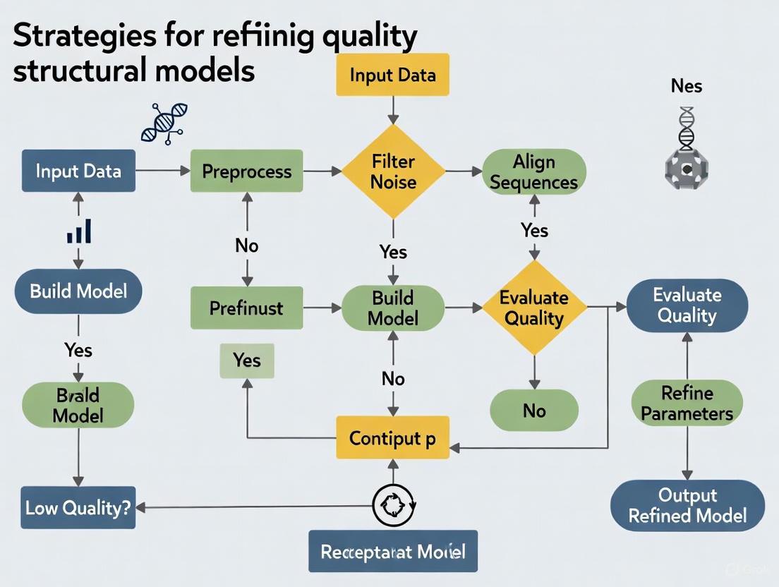
Experimental Workflows for Model Refinement
The following diagrams illustrate standard and modern AI-integrated workflows for structural refinement.
Generic Workflow for Experimental Model Refinement
Workflow for Experimental Model Refinement
AI-Integrated Refinement Workflow
AI-Integrated Refinement Workflow
Research Reagent Solutions
Table 2: Essential Reagents and Tools for Structural Biology Refinement
| Reagent / Tool | Function / Application | Specific Example / Note |
|---|---|---|
| Stable Isotope-labeled Nutrients | Enables NMR spectroscopy of proteins by incorporating detectable nuclei (( ^{15}N ), ( ^{13}C )). | ( ^{15}NH_4Cl ) as a nitrogen source in M9 minimal media [4]. |
| Cross-linking Reagents | Provides distance restraints for structural modeling and validation of complexes via XL-MS. | BS3 (bis(sulfosuccinimidyl)suberate) is a common amine-reactive cross-linker [3]. |
| Cryo-EM Grids | Supports the vitrified sample for imaging in the cryo-electron microscope. | Quantifoil or C-flat grids with ultra-thin carbon film. |
| Detergents & Lipids | Solubilizes and stabilizes membrane proteins for crystallization or cryo-EM. | DDM (n-Dodecyl-β-D-maltoside), LMNG (lauryl maltose neopentyl glycol), Nanodiscs. |
| Protease Inhibitor Cocktails | Prevents proteolytic degradation of sensitive proteins (e.g., IDPs) during purification [4]. | Commercial tablets or solutions containing inhibitors for serine, cysteine, aspartic, and metalloproteases. |
| Rigid Fabs | Stabilizes small or flexible proteins for high-resolution structure determination by cryo-EM [1]. | Disulfide-constrained antibody fragments that limit conformational flexibility of the target protein. |
| AI/ML Software Suites | Predicts protein structures, assists in model refinement, and improves experimental data processing. | AlphaFold2/3, RoseTTAFold, ProteinMPNN, CryoPPP, and various ML-enhanced refinement tools [2] [1]. |
Frequently Asked Questions
Q1: What are the most common types of flaws found in low-quality protein structural models? Low-quality protein models typically exhibit two primary categories of flaws. The first involves backbone inaccuracies, where the main chain trace of the protein is incorrect, leading to a high Root Mean Square Deviation (RMSD) from the native structure. The second common flaw involves side-chain collisions, where the atoms of amino acid side chains are positioned too close together, resulting in steric clashes and unrealistic atomic overlaps that violate physical constraints [5] [6].
Q2: Why is structure refinement particularly challenging for protein complexes compared to single-chain proteins? Refining protein complexes is more difficult because it requires correcting conformational changes at the interface between subunits without adversely affecting the already acceptable quality of the individual subunit structures. Methods that allow backbone movement risk increasing the interface RMSD, while conservative, backbone-fixed methods focusing only on side-chains may be insufficient for correcting larger interfacial errors [5].
Q3: How can I assess the quality of a refined protein model? Quality assessment uses multiple metrics. The fraction of native contacts (fnat) is a straightforward metric for interface quality in complexes. For backbone accuracy, the Root Mean Square Deviation (RMSD) is used, though it is difficult to improve via refinement. Steric clashes are evaluated using tools like the MolProbity clashscore, and overall model quality can be checked with Ramachandran plot analysis and statistical potentials [5] [7] [8].
Q4: My refinement protocol made the side-chains worse. What could have gone wrong? This can occur if the refinement method's energy function or sampling protocol is inadequate. Over-aggressive optimization without proper restraints can lead to side-chain atoms becoming trapped in unrealistic, high-energy conformations or creating new collisions. Using more conservative protocols, applying restraints, or trying a method specifically designed for side-chain repacking like SCWRL or OSCAR-star may yield better results [5].
Q5: Are machine learning methods useful for protein structure refinement? Yes, machine learning is an emerging and powerful tool for refinement. Deep learning frameworks can predict per-residue accuracy and distance errors to guide refinement protocols [6]. Other methods use graph neural networks to directly predict refined structures or estimate inter-atom distances to guide conformational sampling, showing promise in improving both backbone and side-chain accuracy [6].
Troubleshooting Guides
Problem: High Backbone RMSD After Refinement
Description The overall fold or the interface backbone of your model has deviated further from the correct native structure after a refinement procedure.
Diagnosis Steps
- Quantify the Problem: Calculate the global and interface RMSD of your refined model against a known native structure (if available) or a trusted reference model.
- Check Method Type: Determine if you used a backbone-mobile method (e.g., Galaxy-Refine-Complex, PREFMD) or a backbone-fixed method (e.g., Rosetta FastRelax, SCWRL). High RMSD increases are more common with backbone-mobile methods [5].
- Verify Restraints: Check if your refinement protocol allowed for excessive backbone movement without applying sufficient restraints to preserve the overall fold.
Solution
- For critical applications where the initial backbone placement is already good, consider switching to a backbone-fixed refinement method that only repositions side-chains. This prevents the backbone from moving in a wrong direction [5].
- If backbone adjustment is necessary, use methods that incorporate restrained molecular dynamics or evolutionary algorithms for better conformational sampling. Memetic algorithms that combine global search with local optimization can better sample the energy landscape without drastic deviations [6].
- Implement multi-objective optimization strategies that simultaneously optimize different energy functions (e.g., RWplus, Rosetta, CHARMM) to maintain a balance between various structural quality metrics [6].
Problem: Steric Clashes and Side-Chain Collisions
Description The refined model shows atomic overlaps where non-bonded atoms are positioned closer than their van der Waals radii allow, leading to high energy and unstable structures.
Diagnosis Steps
- Identify Clashes: Use validation software like MolProbity to generate a clashscore and visualize specific atomic collisions in a molecular viewer [7].
- Analyze Location: Determine if clashes are localized at the protein-protein interface or scattered throughout the core. Interface clashes are common in unrefined docking models [5].
Solution
- Employ refinement methods with explicit repulsion energy terms (e.g., the
fa_repterm in Rosetta's Ref2015 energy function) that actively penalize atomic overlaps [6]. - Use dedicated side-chain repacking tools like SCWRL or OSCAR-star, which are designed to place side-chains in rotameric conformations that avoid steric clashes [5].
- For persistent clashes, run short cycles of combined side-chain perturbation and restrained relaxation, as implemented in protocols like Galaxy-Refine-Complex [5].
Problem: Refinement Worsens Model Quality Metrics
Description After refinement, key quality metrics like the fraction of native contacts (fnat) decrease, or the model fails a greater number of validation checks.
Diagnosis Steps
- Compare Pre- and Post-Refinement: Systematically calculate a set of quality metrics (fnat, RMSD, clashscore, Ramachandran outliers) for both the initial and refined model.
- Benchmark Method Performance: Consult literature to understand the strengths and weaknesses of your chosen refinement method. Some methods are more adept at improving fnat but may struggle with backbone-dependent metrics like RMSD [5].
Solution
- If the initial model is of high quality, a conservative refinement that primarily optimizes side-chains is often the safest choice to retain the model's merits [5].
- For lower-quality starting models, consider ensemble refinement, where multiple refinement methods are applied, and the best output is selected based on a combination of energy scores and quality metrics [8].
- Utilize quality assessment programs (MQAPs) like GOBA or ProQ that can evaluate the compatibility between the model and the expected protein function or sequence to select the most plausible refined structure [8].
Problem: Refinement of Large Protein Complexes Fails
Description The refinement protocol crashes, produces errors, or yields unrealistic models when applied to multi-chain protein complexes.
Diagnosis Steps
- Check System Size: Large complexes can be computationally prohibitive for some methods. Check the limitations of the software.
- Inspect Subunit Interfaces: Ensure that the initial positioning of the subunits is physically plausible before refinement.
Solution
- For very large complexes, extract a smaller subcomplex containing the key interfaces of interest for refinement, as was done for a homo decamer in a CAPRI benchmark study [5].
- Use refinement methods specifically designed for complexes, such as those incorporating Equivariant Graph Refiner (EGR) models, which can handle the interdependent movements of multiple chains [6].
- Apply interface-specific restraints during refinement to maintain the correct relative orientation of subunits while allowing for flexibility at the interaction surface.
Experimental Protocols & Data
Table 1: Performance of Refinement Method Categories on Common Flaws
| Method Category | Example Protocols | Strengths | Weaknesses | Ideal Use Case |
|---|---|---|---|---|
| Backbone-Mobile | Galaxy-Refine-Complex [5], PREFMD [5], CHARMM Relax [5], Memetic Algorithms (Relax-DE) [6] | Can correct backbone inaccuracies; improves structural flexibility and fnat [5] [6] | High risk of increasing backbone RMSD; computationally intensive [5] | Low-quality models with significant backbone deviations; initial sampling stages |
| Backbone-Fixed | Rosetta FastRelax [5], SCWRL [5], OSCAR-star [5] | Efficiently resolves side-chain collisions; low risk of disrupting correct backbone [5] | Cannot fix backbone errors; limited to side-chain and rotamer optimization [5] | High-quality backbone models requiring side-chain optimization |
| Machine Learning / Deep Learning | ATOMRefine [6], EGR for Complexes [6], RefineD [5] | Rapid prediction of refined structures; can improve both backbone and side-chains [6] | Dependent on training data; "black box" nature can make debugging difficult [6] | Integrating predictive power with sampling-based refinement |
Table 2: Key Quality Metrics for Diagnosing Model Flaws
| Metric | Formula / Calculation | What It Diagnoses | Target Value (Ideal) |
|---|---|---|---|
| RMSD (Backbone) | √[ Σ(atomi - nativei)² / N ] | Overall global or local backbone accuracy. Lower is better [5]. | < 2.0 Å (High Accuracy) |
| Fraction of Native Contacts (fnat) | (Native Contacts in Model) / (Total Native Contacts) | Correctness of inter-subunit interfaces in complexes. Higher is better [5]. | > 0.80 (High Quality) |
| Clashscore | Number of steric clashes per 1000 atoms | Steric hindrance and unrealistic atomic overlaps. Lower is better [7]. | < 5 (High Quality) |
| Ramachandran Outliers | % of residues in disallowed regions of Ramachandran plot | Backbone torsion angle plausibility. Lower is better [7]. | < 1% (High Quality) |
Protocol: Structure Refinement Using a Memetic Algorithm (Relax-DE) [6]
- Initialization: Generate an initial population of structural decoys by applying small perturbations to the atomic coordinates of the low-quality input model.
- Evolutionary Loop:
- Mutation & Crossover: Use Differential Evolution (DE) operators to create new candidate structures by combining and modifying existing ones in the population.
- Local Refinement (Memetic Step): For each new candidate, apply the Rosetta Relax protocol. This performs local energy minimization, focusing on side-chain repacking and backbone adjustments using the full-atom Ref2015 energy function, which includes terms for steric repulsion (
fa_rep), hydrogen bonding, and solvation. - Selection: Evaluate the energy of the refined candidates using the Ref2015 scoring function and select the best-performing structures for the next generation.
- Termination: Repeat the evolutionary loop for a fixed number of generations or until convergence. The lowest-energy structure is selected as the refined model.
Protocol: Gene Ontology-Based Assessment (GOBA) for Model Validation [8]
- Functional Similarity Calculation: For the target protein, obtain a set of functionally similar proteins from databases using its Gene Ontology (GO) terms. Calculate semantic similarity between GO annotations of the target and other proteins using Wang's algorithm.
- Structural Similarity Calculation: Use the Dali structural comparison tool to measure the structural similarity (Z-score) between the model being assessed and each protein in the functionally similar set.
- Quality Score Calculation: The final GOBA score is the weighted sum of the Dali Z-scores, where the weights are the functional similarity scores. A high GOBA score indicates that the model is structurally similar to proteins of similar function, suggesting high quality.
The Scientist's Toolkit: Research Reagent Solutions
| Tool / Resource | Type | Primary Function | Reference |
|---|---|---|---|
| Rosetta Relax | Software Suite | Full-atom, energy-based refinement of side-chains and backbone using Monte Carlo and minimization techniques. | [5] [6] |
| Galaxy-Refine-Complex | Web Server / Software | Refinement of protein complexes via iterative side-chain perturbation and restrained molecular dynamics. | [5] |
| SCWRL4 | Software Algorithm | Fast, accurate side-chain conformation prediction and placement based on a graph theory approach. | [5] |
| MolProbity | Validation Service | Structure validation tool that identifies steric clashes, Ramachandran outliers, and other geometry issues. | [7] |
| GOBA | Quality Assessment | Single-model quality assessment program that scores models based on structural similarity to functionally related proteins. | [8] |
| AutoDock Vina | Docking Software | Used for high-throughput virtual screening to generate initial poses for ligands in structure-based drug design. | [9] |
| Modeller | Software | Homology modeling to generate initial 3D structural models from a target sequence and a related template structure. | [9] |
| PDB | Database | Repository for experimentally determined 3D structures of proteins and nucleic acids, used as templates and benchmarks. | [7] [6] |
Workflow and Pathway Visualizations
Diagram 1: Protein model refinement and troubleshooting workflow.
The Sampling and Scoring Paradigm in Conformational Optimization
Frequently Asked Questions (FAQs)
FAQ 1: Why does my docking or structure prediction algorithm fail to identify near-native structures even after extensive sampling?
This common failure often stems from the decoupling of sampling and scoring [10]. Your sampling step may use a simplified, computationally efficient scoring function to explore the conformational space, while your final scoring uses a more sophisticated function. If these two functions are not well-aligned, the low-energy regions identified during sampling may not correspond to the true low-energy, near-native conformations [10] [11]. Essentially, the sampling function may guide the search away from the correct region of the conformational landscape.
- Solution: Aim for better integration between sampling and scoring. Consider using a more accurate energy function during the later stages of sampling or employing a search algorithm like Model-Based Search (MBS), which builds a model of the energy landscape during search to guide exploration more effectively [11].
FAQ 2: What is the difference between "perturbation-based" and "docking-based" decoys, and why does it matter?
Decoys are non-native structures used to test and develop scoring functions. The method used to generate them is critical:
- Perturbation-based decoys are created by slightly misplacing components of a known native structure [10].
- Docking-based decoys are generated by performing actual docking simulations, often starting from the unbound (separately crystallized) structures of the components [10].
- Solution: For developing methods aimed at realistic docking problems, docking-based decoys are superior. Perturbation-based decoys can be artificially easy for scoring functions to discriminate and do not represent the true challenges of a docking search, potentially leading to over-optimistic results and poorly performing scoring functions in practice [10].
FAQ 3: How can I improve the coverage of conformational space for a highly flexible ligand?
A key challenge is the combinatorial explosion of possible conformers as the number of rotatable bonds increases [12]. Traditional systematic methods become computationally infeasible, while purely stochastic methods may yield non-deterministic results.
- Solution: Consider algorithms that treat rotatable bonds unequally based on their contribution to conformational change. The ABCR (Algorithm based on Bond Contribution Ranking) algorithm, for example, ranks and processes rotatable bonds in batches, focusing computational resources on bonds that have the largest impact on the overall conformation, which can lead to more efficient global sampling [12].
FAQ 4: My sampling algorithm finds a low-energy conformation, but it is far from the native structure. What is the likely cause?
This discrepancy often points to an inaccuracy in the energy function itself [11]. If the scoring function does not correctly describe the physical interactions that stabilize the native complex, the global minimum of the in silico energy landscape will not align with the biologically relevant structure.
- Solution: This failure can be used to identify weaknesses in your energy function. Furthermore, to increase confidence in your results, employ a strategy like the "Wisdom of the Crowds"—using multiple docking programs and combining their results can sometimes compensate for the weaknesses of any single program or scoring function [13].
Troubleshooting Guides
Issue: Poor Performance in Identifying Correct Poses (Low Success Rate)
| Potential Cause | Diagnostic Steps | Resolution |
|---|---|---|
| Weak Scoring Function | Check if the correct pose is generated during sampling but poorly ranked [13]. | Use a consensus scoring approach (e.g., United Subset Consensus) or re-train your scoring function on more realistic, docking-based decoy sets [10] [13]. |
| Inadequate Sampling | Analyze if the conformational search is restricted. | Increase sampling diversity; use algorithms like Model-Based Search or check for a high number of ligand rotatable bonds, which can hinder sampling [11] [13]. |
| Use of Bound Decoys | Review the origin of your training/validation decoy set. | Replace decoys generated from bound (co-crystallized) structures with those from unbound docking, as they present a more realistic challenge [10]. |
Issue: Inefficient Sampling (High Computational Cost, Low Yield)
| Potential Cause | Diagnostic Steps | Resolution |
|---|---|---|
| Combinatorial Explosion | Monitor the number of generated conformers versus rotatable bonds [12]. | Implement a focused sampling algorithm like ABCR that ranks rotatable bonds by contribution and processes them in batches to optimize the search [12]. |
| Rugged Energy Landscape | Observe if the search gets trapped in local minima frequently. | Utilize search methods like replica exchange Monte Carlo or basin hopping that are designed to escape local minima [11]. |
| Over-reliance on Smoothing | Check if early search stages use an oversimplified energy function. | Integrate more accurate, all-atom energy information earlier in the search process, as demonstrated in Model-Based Search [11]. |
Table 1: Performance Comparison of Docking Programs in Pose Identification Data based on a benchmark of 100 protein-ligand complexes from the DUD-E dataset [13].
| Docking Program | Correct Poses Found (Sampling) | Correct Poses Ranked Top-1 (Scoring) | Correct Poses Ranked Top-4 (Scoring) |
|---|---|---|---|
| Surflex | 84 | 59 | 73 |
| Glide | 83 | 68 | 75 |
| Gold | 80 | 61 | 71 |
| FlexX | 77 | 54 | 66 |
| USC Consensus | Information Missing | Information Missing | 87 |
Table 2: Conformer Generation Efficiency of the ABCR Algorithm The ABCR algorithm was evaluated on a dataset of 100 ligands with high flexibility [12].
| Metric | ABCR Performance | Comparative Notes |
|---|---|---|
| RMSD to Crystal Structure | ~1.5 Å (Average, after optimization) | Achieved lower RMSD compared to other methods like Balloon and ETKDG on the same dataset [12]. |
| Number of Conformers Generated | Relationship with rotatable bonds controlled (See Eq. 1 [12]) | Designed to find optimal conformers with fewer generated structures, avoiding combinatorial explosion. |
Experimental Protocols
Protocol 1: Model-Based Search for Conformation Space Search
This protocol outlines the use of Model-Based Search (MBS) for protein structure prediction, which integrates accurate energy functions with intelligent search [11].
- Initialization: Begin with a set of random or heuristic-based initial protein conformations.
- Iterative Model Building and Sampling:
- Execute Sampling Steps: Perform a limited number of conformational search steps (e.g., using Monte Carlo moves).
- Update the Model: Aggregate information from all sampled conformations to build a model that approximates the energy landscape. This model predicts which regions of the conformation space are most promising.
- Guide Exploration: Use the model to select the next regions for exploration, focusing computational resources on areas with a high probability of containing low-energy, near-native structures.
- Refinement: The final set of promising conformations is refined using a high-fidelity, all-atom energy function.
Protocol 2: United Subset Consensus (USC) for Improved Docking
This protocol uses a consensus strategy to improve the chances of finding a correct pose [13].
- Individual Docking: Run docking simulations for the same ligand-protein system using multiple independent programs (e.g., Gold, Glide, Surflex, FlexX).
- Pose Collection: Collect all generated poses from all programs into a single, unified set.
- Consensus Identification: Identify poses that are geometrically similar across the different programs. These consensus poses are considered more reliable.
- Re-ranking: Create a shortlist of top poses based on their consensus across programs. This method can identify correct poses that individual programs might rank poorly.
Workflow and Relationship Diagrams
Diagram 2: The Integrated MBS Workflow
The Scientist's Toolkit: Research Reagent Solutions
Table 3: Essential Resources for Conformational Optimization Research
| Resource / Tool | Type | Primary Function | Key Consideration |
|---|---|---|---|
| ZDOCK/ZRANK | Docking Program & Scoring | Generates decoy sets and provides scoring functions for protein-protein docking [10]. | Decoy sets available online are often generated from unbound structures, making them realistic for method development [10]. |
| RosettaDock | Docking Suite | Provides a flexible framework for protein docking and scoring, including various sampling and scoring protocols [10]. | Includes decoy sets based on both perturbation and unbound docking [10]. |
| DOCKGROUND | Database | Provides a repository of benchmark docking decoy sets for the community [10]. | Useful for obtaining standardized decoy sets for fair comparison of different scoring functions [10]. |
| ABCR | Conformer Generation Algorithm | Optimizes conformer generation for small molecules by focusing on rotatable bonds with the highest impact [12]. | Helps avoid combinatorial explosion and can be used with any user-specified scoring function [12]. |
| Model-Based Search (MBS) | Search Algorithm | A conformation space search method that uses a model of the energy landscape to guide exploration [11]. | Designed to work effectively with accurate, all-atom energy functions, improving prediction accuracy [11]. |
Energy Landscapes and the Thermodynamic Hypothesis of Protein Folding
Theoretical Foundations: FAQs
FAQ 1: What is the thermodynamic hypothesis of protein folding?
The thermodynamic hypothesis, also known as Anfinsen's dogma, states that for a small globular protein under physiological conditions, the native three-dimensional structure is uniquely determined by its amino acid sequence [14]. This native state corresponds to the conformation with the lowest Gibbs free energy, making it the most thermodynamically stable arrangement. The hypothesis requires that the native state is both unique (no other configurations have comparable energy) and kinetically accessible (the protein can reliably find this state without getting trapped) [14].
FAQ 2: How does the energy landscape theory explain the speed of protein folding?
The energy landscape theory visualizes protein folding not as a single pathway, but as a funnel-shaped energy landscape [15] [16]. At the top of the funnel, the unfolded protein has high conformational entropy and high free energy. As it folds, it samples a narrowing ensemble of partially folded structures, progressively losing entropy but gaining stability through native contacts, until it reaches the low-energy native state at the funnel's bottom [16]. This "funnel" concept resolves Levinthal's paradox by showing that proteins do not need to randomly sample all possible conformations; instead, the biased nature of the landscape guides them efficiently toward the native state through a multitude of parallel routes [15] [16].
FAQ 3: What causes protein misfolding and aggregation?
A perfectly "funneled" landscape would lead directly to the native state. However, real landscapes are often rugged, containing non-native local energy minima where folding can become transiently trapped [16] [14]. These kinetic traps arise from conflicting structural interactions, known as frustration [15] [16]. When partially folded structures with exposed hydrophobic surfaces become trapped in these minima, they can interact incorrectly with other molecules, leading to aggregation. In diseases like Alzheimer's and Parkinson's, proteins misfold into stable, alternative conformations (e.g., amyloids) that are thermodynamically stable but pathological, representing exceptions to the classic Anfinsen's dogma [14].
Troubleshooting Guides for Structural Refinement
Problem: My experimental structural model has poor stereochemistry and Ramachandran statistics after low-resolution refinement.
Solution: Apply external restraints to stabilize refinement.
- Diagnosis: Low-resolution experimental data (e.g., from cryo-EM or X-ray crystallography) results in a small ratio of observations to adjustable atomic parameters, making refinement unstable [17].
- Action Plan: Utilize automated pipelines like LORESTR (Low-Resolution Structure Refinement), which is designed for such cases [17].
- Generate Restraints: Use a tool like ProSMART to generate external restraints. These can be based on:
- Homologous structures with known high-resolution models.
- Generic geometric restraints for stabilizing secondary structure elements [17].
- Execute Refinement: Feed these restraints into refinement programs such as REFMAC5 [17].
- Protocol Selection: If the optimal protocol is unclear, LORESTR can execute multiple refinement instances in parallel to identify the best-performing one automatically [17].
- Generate Restraints: Use a tool like ProSMART to generate external restraints. These can be based on:
Table 1: Key Software Tools for Low-Resolution Refinement
| Tool Name | Primary Function | Role in Refinement Workflow |
|---|---|---|
| LORESTR | Automated Pipeline | Executes multiple refinement protocols, auto-detects twinning, and selects optimal solvent parameters [17]. |
| ProSMART | Restraint Generation | Generates external restraints using homologous structures or generic geometry to stabilize the model [17]. |
| REFMAC5 | Refinement Program | Performs the atomic model refinement against experimental data, stabilized by the provided restraints [17]. |
| Rosetta | Refinement & Rebuilding | Uses a Monte Carlo method to refine models guided by cryo-EM density maps, capable of extensive rebuilding [18]. |
Problem: I have a low-resolution Cryo-EM map and an initial Cα trace or comparative model that is inaccurate.
Solution: Use a rebuild-and-refine protocol guided by the density map.
- Diagnosis: Initial models, whether from hand-tracing density or comparative modeling, often contain errors in backbone tracing and side-chain placement that cannot be fixed by minor adjustments [18].
- Action Plan: Implement a protocol based on the Rosetta structure refinement methodology [18].
- Guided Sampling: Augment the Rosetta energy function with a term that quantifies the fit between the atomic model and the experimental density map.
- Extensive Rebuilding: The protocol should not just refine but also rebuild regions identified as incompatible with the experimental density.
- Validation: Test this on a benchmark case. For example, refining the equatorial domain of GroEL from a 4.2Å cryo-EM map and a Cα trace improved the Cα RMSD of helical regions from 3.4Å to 2.2Å [18].
Table 2: Quantitative Benchmarking of Rosetta Refinement into Cryo-EM Maps
| Protein (PDB Code) | Number of Residues | Lowest-RMSD Starting Model (Å) | Lowest-Energy Refined Structure (5Å Map) (Å) |
|---|---|---|---|
| 1c2r | 115 | 3.45 / 4.15 | 0.54 / 1.12 |
| 1dxt | 143 | 2.02 / 2.78 | 0.50 / 1.14 |
| 1onc | 101 | 2.23 / 2.97 | 0.81 / 1.92 |
| 2cmd | 310 | 2.50 / 3.42 | 1.80 / 2.63 |
Table note: RMSD values are presented as Cα RMSD / all-atom RMSD relative to the native crystal structure. Data adapted from Rosetta refinement tests using synthesized 5Å density maps [18].
Experimental Protocols
Protocol 1: Refining a Comparative Model into a Low-Resolution Density Map
Objective: To improve the accuracy of a protein model built by homology (comparative modeling) using a low-resolution (e.g., 5-10Å) cryo-EM density map.
Materials:
- Software: Rosetta software suite [18].
- Inputs:
- The initial comparative model (e.g., generated by a threading algorithm like Moulder or GenThreader).
- The experimental cryo-EM density map in a standard format (e.g., .mrc).
Method:
- Preparation: Convert the density map to the required format for Rosetta, if necessary.
- Input Configuration: Prepare a Rosetta configuration script that specifies:
- The path to the starting model (PDB format).
- The path to the density map file.
- The resolution of the map.
- The weight of the fit-to-density term relative to the standard Rosetta energy function.
- Refinement Execution: Run the Rosetta refinement protocol. This typically involves:
- Monte Carlo Sampling: The algorithm will make random changes to the protein's conformation (e.g., side-chain rotations, small backbone moves).
- Density-Guided Optimization: Each proposed conformational change is evaluated based on the combined score of the physical energy and the fit-to-density. Moves that improve the score are accepted.
- Focused Rebuilding: Regions with poor fit-to-density are targeted for more extensive conformational sampling and rebuilding.
- Model Selection: Upon completion, Rosetta generates thousands of models. Select the final model based on:
- The lowest combined Rosetta energy and fit-to-density score.
- The best correlation coefficient with the experimental density.
- Good stereochemical quality [18].
Protocol 2: Generating and Using External Restraints for Low-Resolution Refinement
Objective: Stabilize the refinement of an atomic model against low-resolution data using prior information from homologous structures.
Materials:
- Software: LORESTR pipeline, ProSMART, REFMAC5 [17].
- Inputs:
- Your atomic model in PDB format.
- The experimental data (e.g., structure factors for crystallography).
- (Optional) One or more homologous high-resolution structures. If not provided, LORESTR can run an automated BLAST search to fetch them from the PDB [17].
Method:
- Pipeline Setup: Input your model and data into the LORESTR pipeline.
- Automated Analysis: LORESTR will perform:
- Auto-detection of crystal twinning.
- Selection of the optimal data scaling method and solvent model parameters.
- If no homologues are provided, it will automatically search for and download suitable structures.
- Restraint Generation: ProSMART will analyze the provided homologous structures to generate positional restraints for your model, tethering it to geometrically plausible conformations.
- Parallel Refinement: LORESTR will launch multiple instances of REFMAC5, each using a slightly different refinement protocol (e.g., varying restraint weights).
- Output Analysis: The pipeline evaluates all refined models based on R-factors, geometry, and Ramachandran plot statistics, and selects the best-performing one for the user [17].
Conceptual Diagrams
Protein Folding Funnel
The Scientist's Toolkit: Research Reagent Solutions
Table 3: Essential Resources for Structural Refinement Research
| Resource Category | Specific Tool / Database | Function in Research |
|---|---|---|
| Structural Databases | Protein Data Bank (PDB) | Primary repository for experimentally determined macromolecular structures, used for obtaining homologues and prior information for refinement [19]. |
| AlphaFold Protein Structure Database | Provides over 200 million highly accurate predicted protein structures, useful as starting models or as references for restraint generation [20]. | |
| Refinement Software | Rosetta | A versatile software suite for structural modeling and refinement, particularly powerful for rebuilding and refining models into cryo-EM density maps [18]. |
| REFMAC5 / ProSMART / LORESTR | A combination of refinement program, restraint generator, and automated pipeline specifically optimized for low-resolution data [17]. | |
| Validation & Analysis | PDB Validation Reports | Provides standardized metrics on model quality, including Ramachandran plot statistics, side-chain rotamer outliers, and clashscores, crucial for assessing refinement outcomes [19]. |
| MolProbity | A widely used structure-validation web service that provides comprehensive analysis of stereochemical quality [19]. |
Limitations of Library-Based Stereochemical Restraints in Conventional Refinement
FAQs: Troubleshooting Common Refinement Problems
FAQ 1: Why does my refined model of a novel ligand have poor geometry, even though the electron density fit seems acceptable?
This is a classic symptom of inadequate stereochemical restraints. Conventional refinement relies on a pre-generated CIF (Crystallographic Information File) restraint library for ligands. This library is based on the ligand's ideal, unbound geometry and does not account for protein-induced strain or specific chemical environments in the active site [21] [22]. The refinement forces the ligand to fit the density while adhering to these idealized restraints, often resulting in strained bond lengths and angles.
- Solution: Utilize refinement methods that incorporate more robust energy functionals. Quantum-mechanical (QM) refinement, for example, calculates stereochemical restraints on-the-fly based on the ligand's specific atomic environment, eliminating the need for an a priori CIF file and producing more chemically accurate models [21].
FAQ 2: My low-resolution structure refinement resulted in distorted protein geometry. What went wrong?
At low resolution, the experimental data is insufficient to determine all atomic parameters accurately. The refinement relies more heavily on the prior knowledge encoded in the stereochemical restraints [23]. Standard library restraints are limited to covalent geometry (bonds, angles, etc.) and lack meaningful terms for non-covalent interactions that stabilize secondary and tertiary structures, such as hydrogen bonds and π-stacking [24]. This can lead to distorted backbone torsion angles and implausible side-chain rotamers.
- Solution: Incorporate additional restraints on the protein backbone and side chains. Tools within refinement suites like PHENIX or REFMAC5 allow you to apply restraints for hydrogen bonding, Ramachandran preferences, and rotamer states [24]. For a more fundamental solution, consider AI-enabled quantum refinement (AQuaRef), which uses a machine-learned interatomic potential to maintain superior geometric quality during low-resolution refinement [24].
FAQ 3: How can stereochemical errors in a refined model impact downstream drug discovery efforts?
Inaccurate structural models directly mislead structure-based drug design (SBDD). Errors can create:
- False Positives: The model shows a strong interaction (e.g., a hydrogen bond) that does not exist in reality, causing chemists to waste effort optimizing the wrong part of a molecule [22].
- False Negatives: A genuine productive interaction is missed because the ligand or protein side chain is incorrectly modeled [22].
- Inaccurate Binding Affinity Predictions: Computational predictions of binding affinity (scoring) are critically dependent on precise atomic coordinates. Models from conventional refinement have been shown to yield poorer correlations with experimental affinity compared to QM-refined models [22].
FAQ 4: What are the most common sources of stereochemical errors in biomolecular structures?
The most common sources include:
- Ligand Restraint Files (CIFs): Manual creation is error-prone, and even automated tools use ideal gas-phase geometry [21].
- Model Building at Low Resolution: It is difficult to correctly fit atoms into poor or ambiguous electron density.
- Incomplete Models: Missing atoms or residues can cause local strain as the refinement attempts to compensate.
- Incorrect Chirality or Peptide Bond Isomerization: These errors can severely disrupt secondary structure, as demonstrated in molecular dynamics simulations [25].
Troubleshooting Guides
Guide 1: Correcting and Validating Ligand Geometry
Problem: A ligand in the refined model has unusual bond lengths or angles, high B-factors, or poor fit in the density.
Protocol:
- Validate: Run a validation tool like
molprobityor the PDB validation server to identify specific geometric outliers [25]. - Inspect the CIF: Check the ligand restraint file (CIF) for errors. Use a program like
eLBOW(in PHENIX) to generate a new CIF from the ligand's molecular structure [21]. - Consider the Chemistry: Does the strained geometry make chemical sense? Could the ligand be in a different protonation or tautomeric state?
- Re-refine with Advanced Methods:
- Using PHENIX/DivCon: Replace the CIF restraints with a QM/MM functional. This can be done by integrating the DivCon plugin with the standard PHENIX refinement workflow. The QM method will calculate appropriate restraints in real-time [21] [22].
- Using AQuaRef: For a more comprehensive solution, refine the entire structure using the AQuaRef package, which uses a machine-learned quantum potential to guide the refinement without relying on libraries [24].
Guide 2: Improving Protein Geometry in Low-Resolution Refinement
Problem: The refined protein model has poor Ramachandran statistics, many rotamer outliers, or distorted secondary structures.
Protocol:
- Apply Secondary Structure Restraints: In refinement software like REFMAC5 or PHENIX, apply hydrogen-bond restraints and restraints on main-chain φ/ψ angles (Ramachandran restraints) and side-chain χ angles (rotamer restraints) [24] [23].
- Use External Homologous Models: If a high-resolution structure of a homologous protein is available, you can use it to generate external restraints for the low-resolution model, informing the refinement about likely geometries [23].
- Switch to Quantum Refinement: For the most robust results, use a quantum refinement method like AQuaRef. This approach is specifically designed to maintain excellent protein geometry at low resolution, achieving better MolProbity scores and Ramachandran Z-scores than standard methods, with a comparable fit to the experimental data [24].
The table below summarizes quantitative data comparing conventional and advanced refinement methods, demonstrating the impact of moving beyond simple library-based restraints.
Table 1: Comparative Performance of Refinement Methods on Protein-Ligand Structures
| Metric | Conventional Refinement | QM/MM Refinement (e.g., PHENIX/DivCon) | AI-Quantum Refinement (AQuaRef) |
|---|---|---|---|
| Average Ligand Strain | Higher | ~3-fold improvement vs. conventional [22] | Not Specified |
| MolProbity Score | Baseline | On average 2x lower (better) [22] | Superior geometry quality [24] |
| Ramachandran Z-score | Baseline | Not Specified | Systematically superior [24] |
| Handling of Novel Chemistry | Requires error-prone manual CIF creation | No CIF required; handles novel motifs [21] | No library required; handles any chemical entity [24] |
| Key Limitation Addressed | N/A | Fixed, idealized ligand restraints | Limited non-covalent interactions in restraints |
Table 2: Impact of Refinement Method on Drug Discovery Applications
| Application | Outcome with Conventional Refinement | Outcome with QM/MM Refinement |
|---|---|---|
| Binding Affinity Prediction | Poorer correlation with experimental data | Significantly improved correlation [22] |
| Detection of Key Interactions | Prone to false positives and false negatives [22] | More accurate identification of H-bonds and other interactions [22] |
| Proton/Protomer State Determination | Not directly supported | Enabled with tools like XModeScore [22] |
The Scientist's Toolkit: Essential Research Reagents & Software
Table 3: Key Software Tools for Advanced Structural Refinement
| Tool Name | Function | Key Feature |
|---|---|---|
| PHENIX/DivCon [21] [22] | QM/MM X-ray & Cryo-EM Refinement | Replaces CIF restraints with a QM/MM functional during refinement. |
| AQuaRef [24] | AI-Enabled Quantum Refinement | Uses machine-learned interatomic potential for entire-protein refinement. |
| REFMAC5 [23] | Macromolecular Refinement | Bayesian framework allowing use of external restraints from homologous models. |
| MolProbity [24] [25] | Structure Validation | Provides comprehensive validation of stereochemistry, clashes, and rotamers. |
| Coot | Model Building & Fitting | Graphical tool for manual model adjustment and ligand fitting. |
Workflow Visualization: From Conventional to Quantum Refinement
The diagram below illustrates the fundamental differences between the conventional refinement workflow and the advanced quantum refinement workflow.
Diagram 1: Contrasting refinement workflows highlights the manual, iterative nature of conventional methods versus the more automated, chemically-driven quantum approach.
Key Methodologies: Experimental Protocols in Detail
Protocol 1: Quantum Refinement of a Protein-Ligand Structure using PHENIX/DivCon
Purpose: To refine a macromolecular crystal structure containing a ligand, obtaining a model with superior geometry without relying on a pre-defined ligand CIF file.
Detailed Methodology:
- Initial Model Preparation: Begin with your best initial atomic model, solved and partially refined using molecular replacement or other methods.
- Integration with PHENIX: Ensure the DivCon plugin is properly installed and integrated with your PHENIX refinement environment [21].
- Refinement Setup: In the PHENIX refinement interface, select the option to use DivCon for the QM calculations. Define the QM region—typically the ligand and its immediate protein environment (e.g., residues within 5-10 Å).
- Run Refinement: Execute the standard PHENIX refinement macro-cycle. The key difference is that in each micro-cycle, the L-BFGS minimizer will use energy gradients computed by the semiempirical QM (e.g., AM1) method for the defined region instead of gradients from the CIF-based restraints [21]. The target function becomes:
T = Ωxray * Txray + ΩQM * TQM, whereTQMis the QM energy. - Validation: Upon completion, validate the final model using MolProbity. Expect to see lower ligand strain and improved clashscores compared to conventional refinement [22].
Protocol 2: Full-Protein AI-Quantum Refinement using AQuaRef
Purpose: To refine an entire protein structure (e.g., from low-resolution X-ray or cryo-EM data) using a machine-learned quantum potential to achieve optimal geometry.
Detailed Methodology:
- Pre-refinement Checks: The AQuaRef procedure begins with a strict check of the initial model. The model must be atom-complete, correctly protonated, and free of severe steric clashes. Missing atoms must be added, and severe clashes are resolved with quick geometry regularization [24].
- Crystallographic Symmetry Handling (For X-ray): For crystallographic data, the model is expanded into a supercell using space group symmetry operators to account for crystal packing effects. It is then truncated to retain only parts within a specified distance from the main copy [24].
- Refinement Execution: The atom-completed (and potentially expanded) model is refined using the Q|R package within Phenix, which now uses the AIMNet2 machine-learned interatomic potential (MLIP) to calculate restraints. This potential mimics quantum mechanics at a fraction of the computational cost, allowing for linear scaling (O(N)) with system size [24].
- Analysis: The refined model will typically show a superior MolProbity score, better Ramachandran statistics, and a similar or better fit to the experimental data (R-free) compared to models refined with standard or additional restraints [24].
Cutting-Edge Refinement Methodologies: From AI-Driven Potentials to Hybrid Algorithms
AQuaRef Technical Support Center
Troubleshooting Guides
Issue 1: Initial Refinement Fails Due to Severe Geometric Violations
- Problem: The AQuaRef procedure terminates at the initial check, reporting severe geometric violations like steric clashes or broken covalent bonds.
- Cause: AQuaRef requires a stricter initial atomic model compared to standard refinement. The input model must be atom-complete, correctly protonated, and free of major geometric errors [24].
- Solution: Perform quick geometry regularization using standard stereochemical restraints prior to initiating AQuaRef. This step minimally adjusts atoms to resolve clashes without significantly altering the model [24].
Issue 2: Unacceptable Computational Performance or GPU Memory Exhaustion
- Problem: The refinement process is excessively slow or fails due to insufficient GPU memory.
- Cause: While AQuaRef's AIMNet2 potential scales linearly (O(N)) with system size, very large models (>180,000 atoms) may exceed the memory of a single GPU. Performance can also be suboptimal if hardware does not meet recommendations [24].
- Solution:
- Verify your system meets the recommended hardware specifications (see Section 1.3, Essential Research Reagent Solutions).
- For large systems, ensure you are using a GPU with at least 80GB of memory, such as an NVIDIA H100, to accommodate models up to ~180,000 atoms [24].
- Confirm that the AIMNet2 model is being utilized, as it provides quantum-level fidelity at a fraction of the cost of full QM calculations [24] [26] [27].
Issue 3: Poor Fit to Experimental Data After Quantum Refinement
- Problem: The refined atomic model shows excellent geometry but a worsened fit to the experimental data (e.g., higher R-free).
- Cause: The balance between the fit to the experimental data (Tdata) and the quantum-mechanical restraints (Trestraints) may be suboptimal [24].
- Solution: This is an integral part of the refinement protocol managed by the Quantum Refinement package (Q|R). Ensure you are using the latest version of the Q|R package within Phenix, as it is specifically designed to handle this balance during the minimization process [24].
Issue 4: Handling Crystallographic Symmetry and Static Disorder
- Problem: For crystallographic data, the refinement does not correctly account for symmetry-related interactions or models with alternative conformations.
- Cause: Quantum mechanics codes, including the current AQuaRef implementation, do not inherently handle crystallographic symmetry or static disorder [24].
- Solution: For symmetry, the Q|R package automatically expands the model into a supercell using space group symmetry operators and truncates it to include nearby symmetry copies, ensuring these interactions are considered [24]. Handling static disorder remains a limitation and may require reverting to standard refinement techniques for those specific regions.
Frequently Asked Questions (FAQs)
Q1: What are the key advantages of using AQuaRef over standard refinement methods? AQuaRef uses machine learning interatomic potentials (MLIPs) to derive stereochemical restraints directly from quantum mechanics, moving beyond limited library-based restraints. This yields models with superior geometric quality, better handles non-standard chemical entities, and improves the modeling of meaningful non-covalent interactions like hydrogen bonds, all while maintaining a comparable fit to experimental data [24] [26].
Q2: My model is derived from a low-resolution Cryo-EM map. Can AQuaRef improve it? Yes. AQuaRef has been tested on 41 low-resolution cryo-EM atomic models. Results demonstrate systematic improvement in geometric quality, as measured by MolProbity scores and Ramachandran Z-scores, without degrading the fit to the experimental map [24].
Q3: How does AQuaRef assist in determining proton positions? The quantum-mechanical approach of AQuaRef is particularly adept at modeling hydrogen bonds and their associated proton positions. This has been successfully illustrated in challenging cases, such as determining the protonation states of short hydrogen bonds in the protein DJ-1 and its homolog YajL [24] [26].
Q4: What is the typical computational time for a quantum refinement cycle? Performance is structure-dependent. However, for about 70% of the models tested, AQuaRef refinement was completed in under 20 minutes. The maximum time observed was around one hour, which is often shorter than standard refinement that includes additional secondary structure and rotamer restraints [24].
Q5: What are the minimum requirements for an atomic model to be suitable for AQuaRef? The model must be atom-complete (all atoms, including hydrogens, must be present), correctly protonated, and free of severe steric clashes or broken bonds. Models with missing main-chain atoms that cannot be automatically added are not suitable for the current workflow [24].
Quantitative Performance Data
The following tables summarize key quantitative data from the AQuaRef study, which refined 41 cryo-EM and 30 X-ray structures for validation [24].
Table 1: Computational Performance Scaling of AIMNet2 Model
| System Size (Atoms) | Calculation Time (seconds) | Peak GPU Memory | Hardware |
|---|---|---|---|
| ~100,000 atoms | 0.5 s (single-point energy/forces) | Fits within 80GB | NVIDIA H100 GPU |
| Scaling Complexity | Linear (O(N)) for time and memory | Linear (O(N)) for time and memory | - |
Table 2: Geometric Quality Assessment of Refined Models
| Validation Metric | Standard Refinement | Standard + Additional Restraints | AQuaRef (QM Restraints) |
|---|---|---|---|
| MolProbity Score | Baseline | Improved vs. Standard | Superior systematic improvement |
| Ramachandran Z-score | Baseline | Improved vs. Standard | Superior systematic improvement |
| CaBLAM Disfavored | Baseline | Improved vs. Standard | Superior systematic improvement |
| Hydrogen Bond Parameters | Baseline | Improved vs. Standard | Superior (better skew-kurtosis plot) |
Table 3: Model-to-Data Fit for X-ray Structures
| Fit Metric | Standard Refinement | AQuaRef (QM Restraints) |
|---|---|---|
| R-free | Baseline | Similar |
| R-work - R-free gap | Baseline | Smaller (indicates less overfitting) |
Experimental Protocol: AQuaRef Workflow
The AQuaRef workflow integrates machine learning interatomic potentials into the quantum refinement pipeline. The following diagram and detailed methodology outline the procedure as applied in the cited research [24].
Detailed Methodology
- Initial Model Preparation: The process begins with an initial atomic model derived from cryo-EM or X-ray crystallography data. This model is checked for atom completeness. Any missing atoms, including hydrogens, are added to create a fully protonated model. This step may introduce steric clashes, which are identified here [24].
- Geometry Regularization: If severe geometric violations (e.g., steric clashes, broken bonds) are detected, a quick geometry regularization is performed. This step uses standard stereochemical restraints to resolve the violations with minimal atomic displacement, preparing the model for stable quantum refinement [24].
- Crystallographic Symmetry Handling (X-ray only): For crystallographic data, the model is expanded into a supercell by applying relevant space group symmetry operators. This supercell is then truncated to retain only the symmetry copies within a specific cutoff distance from the atoms of the main copy. This ensures that intermolecular interactions from crystallographic symmetry are correctly accounted for during the quantum refinement, which the QM code does not handle natively. This step is bypassed for cryo-EM data [24].
- AQuaRef Minimization: The core refinement is performed using the Q|R (Quantum Refinement) package. The refinement target is minimized, which balances the fit to the experimental data (Tdata) with the quantum-mechanical energy of the system (Trestraints) calculated using the AIMNet2 machine-learned interatomic potential. This MLIP mimics high-level quantum mechanics at a substantially lower computational cost, enabling the refinement of entire proteins [24] [26] [27].
- Output: The result is a refined atomic model that exhibits superior geometric quality while maintaining an equal or better fit to the experimental data compared to models refined with standard methods [24].
The Scientist's Toolkit: Essential Research Reagent Solutions
Table 4: Essential Software and Computational Resources for AQuaRef
| Item Name | Function / Role in the Experiment | |
|---|---|---|
| AIMNet2 MLIP | The machine-learned interatomic potential that provides quantum-mechanical energy and forces for the system at a computational cost that scales linearly with system size, making full-protein refinement feasible [24] [26]. | |
| Quantum Refinement (Q|R) Package | The software package (integrated with Phenix) that manages the quantum refinement workflow, including handling symmetry, balancing the experimental data fit with QM restraints, and performing the minimization [24]. | |
| Phenix Software | A comprehensive Python-based software suite for the automated determination of macromolecular structures using X-ray crystallography and other methods. It provides the framework for the Q | R package [24]. |
| NVIDIA H100 GPU (80GB) | High-performance computing hardware recommended for large refinements. Its substantial memory allows single-point energy and force calculations for systems as large as ~180,000 atoms in about 0.5 seconds [24]. |
Technical Support Center
Frequently Asked Questions (FAQs)
Q1: The energy of my refined protein model is not decreasing, or the optimization appears stuck. What could be wrong? This is often a sampling issue. The memetic algorithm combines global and local search to escape local minima. Ensure your Differential Evolution (DE) parameters are correctly set. A low population size or improperly scaled mutation step can hinder global exploration. Furthermore, verify that the Rosetta Relax protocol is correctly integrated for local refinement; an incorrect energy function weight can prevent meaningful minimization. The "Relax-DE" approach is specifically designed to better sample the energy landscape compared to Rosetta Relax alone [6].
Q2: How do I balance the computational cost between the global DE search and the local Rosetta Relax step? The memetic algorithm is computationally intensive. For initial tests, use a low number of DE generations (e.g., 10-20) and a limited number of Relax cycles (e.g., 3-5). The runtime should be comparable to the reference method you are benchmarking against. Studies show that the Relax-DE memetic algorithm can obtain better energy-optimized conformations in the same runtime as the standard Rosetta Relax protocol [6].
Q3: My refined model has severe atomic clashes after a DE mutation step. How can this be resolved?
Atomic clashes are expected after global mutation operations. This is precisely why the local search component is critical. The integrated Rosetta Relax protocol should be applied to these perturbed decoys to perform local minimization and resolve steric conflicts by optimizing side-chain rotamers and backbone angles [6]. The fa_rep term in the Ref2015 full-atom energy function is specifically designed to penalize such repulsive interactions [6].
Q4: What is the recommended way to assess the success of a refinement run? Success should be evaluated using multiple metrics. The primary metric is the improvement in the full-atom energy score (e.g., Ref2015). However, since the native structure is unknown during prediction, you must also use spatial quality metrics. Calculate the Root-Mean-Square Deviation (RMSD) of your refined models against a trusted reference structure, such as one determined experimentally. A successful refinement yields models with lower energy and comparable or better RMSD [6].
Q5: How does this memetic approach compare to new deep learning-based refinement methods? Deep learning methods, such as those using SE(3)-equivariant graph transformers (e.g., ATOMRefine), can directly refine both backbone and side-chain atoms [6]. The memetic algorithm is a sampling-based optimization approach that excels at navigating complex energy landscapes. The two are not mutually exclusive; future work could explore hybrid models where deep learning provides initial refined guesses for the memetic algorithm to further optimize [6].
Troubleshooting Guides
Issue: Runtime is excessively long.
- Potential Cause 1: Protein target is too large (high number of residues).
- Solution: For large proteins, consider using a coarse-grained representation during the initial DE phases or employing fragmentation approaches [28]. The full-atom refinement with Rosetta Relax can be applied to the most promising decoys in the final stages.
- Potential Cause 2: Population size or number of generations is set too high.
- Solution: Start with smaller values (e.g., population size of 50, 10 generations) and increase gradually as needed. The goal is to find a balance between exploration and computational feasibility.
Issue: Refined models are highly similar (lack diversity).
- Potential Cause: The algorithm has converged to a single local minimum, losing population diversity.
- Solution: Integrate niching methods into the DE algorithm. Techniques such as crowding, fitness sharing, or speciation can maintain a diverse set of optimized conformations, which is crucial for exploring the multimodal energy landscape of protein folding [29].
Issue: Rosetta Relax fails to improve models generated by DE.
- Potential Cause 1: The DE mutation has created a conformation that is too distant from the native fold for local search to recover.
- Solution: Implement a filtering step before applying Relax. Discard decoys with energy scores above a certain threshold or with unrealistic stereochemistry.
- Potential Cause 2: Incorrect setup of the Rosetta Relax protocol.
- Solution: Double-check the configuration files for the refinement protocol. Ensure you are using the appropriate full-atom energy function (Ref2015) and that constraints (if used) are correctly applied [6].
Experimental Protocol: Memetic Algorithm for Protein Refinement
The following workflow details the methodology for refining protein structures using a memetic algorithm that hybridizes Differential Evolution (DE) and the Rosetta Relax protocol [6].
1. Initialization
- Input: A starting 3D structural model of the protein, typically from a low-resolution prediction method like AlphaFold2 or RoseTTAFold.
- Representation: Convert the structure into a full-atom representation, including all side-chain atoms.
- Population Generation: Initialize the DE population by applying small random perturbations (e.g., via "packing" and "minimization" moves in Rosetta) to the side-chain dihedral angles (χ angles) and backbone torsions of the input model. This creates an initial set of diverse decoys.
2. Evaluation
- Energy Calculation: Score each decoy (protein conformation) in the population using the Rosetta full-atom energy function, Ref2015. This function is a weighted sum of ~19 terms, including fa_rep (atom repulsion), electrostatic interactions, and solvation terms [6].
- Fitness Assignment: The raw energy score is typically used as the fitness value to be minimized. Lower energy indicates a more stable, and potentially more native-like, conformation.
3. Differential Evolution (Global Search) The DE algorithm generates new candidate solutions by combining existing ones. For a target vector in the population, a mutant vector is created:
- Mutation: Select three distinct random vectors from the population. The mutant vector is generated according to: ( V{i,g} = X{r1,g} + F \cdot (X{r2,g} - X{r3,g}) ), where ( F ) is the scaling factor.
- Crossover: Create a trial vector by mixing parameters (e.g., torsion angles) from the target vector and the mutant vector based on a crossover probability (CR).
- Selection: The trial vector is evaluated with the energy function. It replaces the target vector in the next generation if it has a lower (better) energy score.
4. Rosetta Relax (Local Search)
- After the DE selection step, the local search is applied. This can be done on all new population members, a selected subset (e.g., the best), or with a certain probability.
- The Rosetta Relax protocol performs a series of alternating side-chain "packing" (optimizing rotamer choices) and gradient-based energy "minimization" steps. This locally optimizes the atom positions to relieve atomic clashes and find the lowest energy conformation in the immediate neighborhood [6].
5. Termination and Output
- The algorithm iterates between steps 2-4 for a predefined number of generations or until convergence is reached (e.g., no significant fitness improvement over several generations).
- The final output is the lowest-energy conformation found and/or an ensemble of diverse, low-energy structures from the final population.
The Scientist's Toolkit: Research Reagent Solutions
Table: Essential computational tools and their functions in memetic algorithm-based protein refinement.
| Item Name | Function / Rationale |
|---|---|
| Rosetta Software Suite | Provides the core energy functions (Ref2015), the Relax protocol for local minimization, and utilities for manipulating protein structures (e.g., perturbing and packing side chains) [6]. |
| Differential Evolution Algorithm | A robust global optimization algorithm that recombines population members to explore the high-dimensional conformational space effectively, helping to avoid local minima [6] [29]. |
| Protein Data Bank (PDB) | A repository of experimentally solved protein structures. Used to obtain high-quality reference structures for validating refinement results and for training knowledge-based energy terms [6]. |
| Niching Methods (Crowding, Speciation) | Algorithms integrated into the DE to maintain population diversity. This is crucial for sampling multiple local minima in the deceptive, multimodal energy landscape of protein folding [29]. |
| Full-Atom Energy Function (Ref2015) | A physics- and knowledge-based scoring function used to evaluate protein conformations. It includes terms for van der Waals repulsion (fa_rep), hydrogen bonding, solvation, and torsional preferences [6]. |
| Trusted Research Environment (TRE) | A secure, controlled computational platform that enables collaborative research on sensitive data (e.g., proprietary protein sequences) without the need for direct data sharing, using techniques like federated learning [30]. |
Table: Key components and parameters in the memetic refinement algorithm.
| Component / Parameter | Description / Typical Value / Function |
|---|---|
| Optimization Goal | Find the 3D atomic coordinates that minimize the full-atom energy function [6]. |
| Algorithm Type | Memetic Algorithm (Hybrid of Differential Evolution and Rosetta Relax) [6]. |
| Protein Representation | Full-atom (includes backbone and all side-chain atoms) [6]. |
| Key Energy Term | fa_rep: Atom-pair repulsion energy, critical for resolving atomic clashes [6]. |
| Reported Advantage | Better samples the energy landscape and finds lower-energy structures in the same runtime compared to Rosetta Relax alone [6]. |
| Validation Metric | Root-Mean-Square Deviation (RMSD) against a native structure; Energy score [6] [29]. |
Method Workflow and Signaling
The following diagram illustrates the integrated workflow of the memetic algorithm, showing how the global and local search components interact.
Memetic Algorithm Refinement Workflow
Machine-Learned Interatomic Potentials (MLIPs) for Quantum-Level Fidelity at Reduced Cost
Frequently Asked Questions (FAQs)
FAQ 1: Why does my MLIP fail to accurately simulate atomic dynamics or rare events, even when it shows low average errors on my test set?
Low average errors, such as root-mean-square error (RMSE) on standard test sets, are insufficient for gauging the performance of MLIPs in molecular dynamics (MD) simulations. These average errors often mask significant inaccuracies for specific atomic configurations that are critical for simulating diffusion, defect migration, or other rare events [31]. Standard training and testing datasets may not adequately sample these transition states. Even when defect structures are included in training, MLIPs can still exhibit large errors in predicting properties like vacancy formation energy and migration barriers [31].
- Solution: Develop and utilize application-specific evaluation metrics. Instead of relying solely on average errors, calculate the force errors specifically on atoms identified as participating in rare events (e.g., a migrating atom during diffusion). Using these targeted "force performance scores" as optimization metrics has been shown to lead to MLIPs with improved prediction of atomic dynamics and diffusional properties [31].
FAQ 2: How can I improve my MLIP's accuracy when my ab initio training data contains inherent inaccuracies or systematic errors?
The accuracy of an MLIP is inherently limited by the accuracy of its training data. If the underlying Density Functional Theory (DFT) data has systematic errors, such as an overestimation of lattice parameters, the MLIP will inherit these inaccuracies [32].
- Solution: Refine pre-trained MLIPs using experimental data. Techniques like differential trajectory re-weighting allow you to fine-tune a DFT-trained MLIP to match experimental observables without overfitting. For example, refining an MLIP against Experimental Extended X-ray Absorption Fine Structure (EXAFS) spectra, which are sensitive to local atomic structure, has been demonstrated to significantly improve the prediction of various structural and thermodynamic properties, bringing them closer to experimental values [32].
FAQ 3: How do I choose the right MLIP architecture for my specific application?
The "best" MLIP architecture depends on a trade-off between accuracy, computational speed, and data efficiency for your specific problem [33]. Newer equivariant architectures generally offer high accuracy but can be more computationally expensive.
- Solution: Consider your application's requirements. For high accuracy in structurally and chemically complex systems, equivariant message-passing graph neural networks like NequIP and MACE are often top performers [33]. If simulation speed is a priority, especially for large systems or long timescales, simpler models like the linear Atomic Cluster Expansion (ACE) or SNAP may be more suitable, as they can achieve near-optimal accuracy with lower computational cost [34]. Benchmarking several architectures on a small subset of your data is a practical approach.
Troubleshooting Guides
Issue 1: Poor Performance on Defect Configurations and Rare Events
Problem: Your MLIP shows low overall errors but fails to accurately simulate processes like vacancy diffusion, surface adatom migration, or other rare events. The MD simulations may become unstable or produce incorrect energy barriers [31].
Diagnosis: This is a common issue indicating that the training dataset does not sufficiently cover the relevant regions of the potential energy surface (PES), particularly the transition states involved in these rare events [31].
Resolution Protocol:
- Identify Critical Configurations: Run short ab initio MD (AIMD) simulations to explicitly generate trajectories containing the rare event of interest (e.g., a vacancy or interstitial migrating through the lattice).
- Create a Specialized Test Set: Extract 100-200 snapshots from these AIMD trajectories to create a dedicated "rare-event testing set" [31].
- Analyze Targeted Errors: Evaluate your current MLIP on this set. Don't just look at average errors; pay specific attention to the force errors on the few atoms that are actively participating in the migration event [31].
- Enhance Training Data: Add these critical snapshots from the rare-event trajectories to your training dataset.
- Retrain with Specific Metrics: During retraining, use optimization metrics that incorporate the force errors on these migrating atoms to guide the model improvement [31].
Issue 2: MLIP Inherits Systematic Errors from DFT Training Data
Problem: Your MLIP's predictions for certain properties (e.g., lattice constant) show consistent, significant deviations from known experimental results, even though the MLIP closely matches the DFT data it was trained on [32].
Diagnosis: The DFT method used to generate the training data has a systematic error, which has been learned and reproduced by the MLIP.
Resolution Protocol (Experimental Refinement):
- Pre-train an MLIP: Begin by training a robust MLIP on your available DFT data using standard active learning procedures to ensure good coverage of the PES [32].
- Select Experimental Observable: Choose a high-quality experimental observable that is sensitive to the property your MLIP gets wrong. EXAFS spectra are an excellent choice for refining local structural environments [32].
- Apply Re-weighting Technique: Use a differential trajectory re-weighting method. This technique re-weights a reference MD trajectory generated with the original MLIP, allowing you to adjust the MLIP's parameters to match the experimental observable without performing a new MD simulation at each step [32].
- Avoid Overfitting: Combine this re-weighting with transfer learning and perform the re-training for only a minimal number of epochs to prevent overfitting to the single experimental data point [32]. This process results in an "EXAFS-refined" MLIP that retains the general knowledge from DFT but is corrected toward experimental accuracy.
The Scientist's Toolkit: Research Reagent Solutions
The table below summarizes key computational tools and methodologies essential for developing and applying MLIPs.
| Research Reagent | Function & Explanation |
|---|---|
| Equivariant Neural Networks (e.g., NequIP, MACE, Allegro) | MLIP architectures that explicitly embed rotational and translational symmetries into the model, leading to superior data efficiency and accuracy for predicting energies and forces [33] [35]. |
| Gaussian Approximation Potential (GAP) | A class of MLIP that uses Gaussian process regression combined with atomic environment descriptors (like SOAP) to learn the potential energy surface [36]. |
| Spectral Neighbor Analysis Potential (SNAP/qSNAP) | An MLIP formalism that expands atomic energies using bispectrum components. Its quadratic extension (qSNAP) offers a good balance of accuracy and computational efficiency [34]. |
| Smooth Overlap of Atomic Positions (SOAP) | A widely used descriptor that provides a quantitative measure of the similarity between local atomic environments, invariant to rotations, translations, and atom permutations [36] [31]. |
| Active Learning (AL) | An automated procedure for generating diverse training datasets. It selects the most informative atomic configurations for DFT calculations, ensuring robust and transferable MLIPs while minimizing computational cost [32] [34]. |
| Differential Trajectory Re-weighting | A technique that allows for the refinement of a pre-trained MLIP using experimental data (like EXAFS) or higher-level theory data, correcting for systematic errors in the original training data [32]. |
This table compares the performance of different MLIP frameworks for structurally and chemically complex systems, highlighting the trade-off between accuracy and computational cost.
| MLIP Architecture | Accuracy (Al-Cu-Zr) | Accuracy (Si-O) | Computational Speed | Key Characteristic |
|---|---|---|---|---|
| MACE | High | High | Medium | High accuracy, equivariant [33] |
| Allegro | High | Medium | Medium | High accuracy, equivariant [33] |
| NequIP | Medium | High | Medium | Equivariant, performs well for Si-O [33] |
| nonlinear ACE | High | Medium | Fast | Strong accuracy-speed trade-off [33] |
| GAP | Medium | Medium | Slow (CPU) | Gaussian process-based [36] [33] |
This table shows how using reduced-precision DFT calculations for training data generation can drastically lower computational cost with minimal impact on final MLIP accuracy for certain applications.
| DFT Precision Level | k-point Spacing (Å⁻¹) | Energy Cut-off (eV) | Avg. Run Time per Config. (sec) | Suitability for MLIP Training |
|---|---|---|---|---|
| 1 (Low) | Gamma only | 300 | 8 | May be sufficient with force weighting [34] |
| 3 (Medium) | 0.75 | 400 | 15 | Good balance of cost and accuracy [34] |
| 6 (High) | 0.10 | 900 | 996 | High cost, marginal gains for some properties [34] |
Workflow Visualization
The diagram below outlines the key decision points and methodologies for developing and refining a robust MLIP.
MLIP Development and Refinement Workflow
Integrating Geometric Cues from Enhanced Textures for 3D Model Consistency
Frequently Asked Questions (FAQs)
Q1: What is the core challenge in achieving 3D model consistency with textured models? The core challenge is the ill-posed nature of reverse projection. When mapping 2D textures onto 3D meshes, multiple 3D faces can map to the same 2D pixel, and crucial spatial information is lost when flattening 3D shapes into 2D UV space. This often results in visible seams, texture misalignment, and the Janus problem (artifacts under diverse viewpoints) [37].
Q2: My model has inconsistent textures across different views. What strategy can help? Framing texture synthesis as a video generation problem is an effective strategy. Video generation models are specifically designed to maintain temporal consistency across frames. By treating different viewpoints or time steps as video frames, these models can enforce smoother transitions and superior spatial coherence across the entire 3D model surface [37].
Q3: How can I repair a 3D model with messy geometry before texturing? A structured geometry repair workflow is essential [38]:
- Start with retriangulation to ensure uniform, high-quality mesh triangles.
- Identify and repair defects like holes, self-intersections, and near-degenerate triangles.
- Ungroup problematic geometries to separate non-manifold or disjointed sections for targeted repair.
- Form closed triangulations to ensure all volume pieces are watertight.
- If issues persist, use Divide All Geometry tool in multiple steps to resolve underlying defects [38].
Q4: Why do occluded or hidden areas of my model have poor texture quality? Occluded areas are often information-poor because they are rarely visible in training views from fixed viewpoints. A component-wise UV diffusion strategy can address this. By decomposing a model into its core components and processing them separately in UV space, this strategy better preserves semantic information and enhances texture quality in these challenging regions [37].
Troubleshooting Guides
Problem 1: Visible Seams at UV Boundaries
| Troubleshooting Step | Description & Rationale | Key Quantitative Metric / Setting |
|---|---|---|
| Employ Geometry-Aware Conditions [37] | Use 3D structure information (normal, depth, and edge maps) during texture generation to align textures precisely with the underlying complex geometry. | Input: Normal, Depth, and Edge maps. |
| Adopt a Component-Wise UV Strategy [37] | Process individual 3D model components separately in UV space. This provides finer control and avoids artifacts caused by fragmented, automated UV cuts. | Method: UV diffusion per model component. |
| Verify Watertight Geometry [38] | Ensure the 3D mesh itself has no gaps. Use the "Form Closed Triangulation" function to make all volume pieces are watertight before texturing. | Tool: Form Closed Triangulation function. |
Problem 2: Texture Inconsistencies Across Different Viewpoints
| Troubleshooting Step | Description & Rationale | Key Quantitative Metric / Setting |
|---|---|---|
| Leverage Video Generation Models [37] | Utilize a framework like VideoTex, which treats texture synthesis as a video generation task to ensure temporal and spatial stability across frames representing different views. | Framework: VideoTex. |
| Integrate Multimodal Information [39] | Fuse structural, texture, and semantic information pipelines during model generation. This holistic approach improves consistency. | Pipeline: 3D Prior Pipeline & Model Training Pipeline. |
| Optimize Triangulation Quality [38] | Poorly triangulated surfaces can cause rendering inconsistencies. Use retriangulation to create a consistent, high-quality mesh. | Tool: Retriangulation function. |
Problem 3: Low-Fidelity Textures on Complex Geometries
| Troubleshooting Step | Description & Rationale | Key Quantitative Metric / Setting |
|---|---|---|
| Use a Structure-wise UV Diffusion [37] | This strategy specifically enhances the generation of occluded areas by preserving semantic information, resulting in smoother and more coherent textures across complex shapes. | Strategy: Structure-wise UV diffusion. |
| Simplify Model Geometry [38] | Avoid unnecessary complexity. For instance, overlapping structures can be unified into a single convex volume, reducing computational cost without sacrificing accuracy. | Guideline: Simplify convex volumes. |
| Assign Materials Early [38] | Assign material properties to geometries before dividing them. This ensures logical continuity and avoids time-consuming fixes later in the process. | Workflow: Early material assignment. |
Experimental Protocols & Methodologies
Protocol 1: Evaluating Texture Seam Consistency
Objective: To quantitatively assess the visual smoothness and coherence of synthesized textures across UV map boundaries.
Methodology:
- Synthesis: Generate textures using a component-wise UV diffusion strategy that processes individual 3D model components separately in UV space [37].
- Viewpoint Rendering: Render the textured 3D model from multiple, evenly distributed viewpoints.
- Boundary Analysis: For each rendering, apply an edge-detection algorithm specifically focused on the pre-defined UV seam locations.
- Metric Calculation: Calculate the Seam Visibility Index (SVI) for each rendered view [37]:
SVI = (Total edge strength at UV seams) / (Total edge strength across entire image) - Comparison: Compare the average SVI across all views against models textured with baseline methods (e.g., fixed viewpoint inference).
Protocol 2: Testing Viewpoint Consistency Using a Hexagonal Room Paradigm
Objective: To evaluate and train the ability of a system to reorient itself using geometric cues versus simple landmark features.
Methodology:
- Environment Setup: Use a serious game environment based on a hexagonal virtual room with a tiled floor, textured walls, and landmark objects [40].
- Cue Manipulation:
- The target location is always geometrically defined.
- Landmarks are progressively removed over training levels.
- The room is rotated between trials, changing the user's viewpoint [40].
- Data Logging: System tracks all errors during the search for the target. Errors are categorized into three types [40]:
- Nearby Error: Choosing a tile adjacent to the target's segment.
- Nearby Corner Error: Choosing a tile at the corner between the target's segment and an adjacent one.
- Side Error: Choosing a tile in a completely different segment.
- Analysis: Monitor the change in error types and frequency over repeated sessions to quantify the learning of geometric cue integration over feature reliance [40].
Workflow Visualization
Geometric Consistency Workflow
Texture Synthesis as Video Generation
The Scientist's Toolkit: Research Reagent Solutions
| Essential Material / Tool | Function in Research |
|---|---|
| Video Generation Model [37] | Serves as the core engine for texture synthesis, ensuring temporal and spatial consistency across different viewpoints by treating them as video frames. |
| Geometry-Aware Conditions [37] | Inputs such as normal, depth, and edge maps that provide the diffusion model with critical 3D structural information, ensuring textures align with geometry. |
| Component-Wise UV Diffusion Strategy [37] | A methodological approach that decomposes a 3D model into its components for individual texturing in UV space, significantly enhancing quality in occluded areas and across seams. |
| 3D Diffusion Model (e.g., G3D) [39] | Used to generate a rough 3D prior, gradually recovering an object's geometric shape, texture details, and semantic information through a denoising process. |
| Structured Repair Workflow [38] | A systematic sequence of operations (Retriangulation -> Repair Defects -> Form Closed Triangulation) for preparing and cleaning messy 3D geometries before texturing. |
| Hexagonal Room Paradigm [40] | A validated serious game environment for evaluating and training spatial reorientation skills and the integration of geometric cues versus feature cues. |
Troubleshooting Guides
Protonation State Determination
Problem: My refinement shows unexplained electron density and poor geometry around active site residues. How do I determine the correct protonation state?
Solution: Unexplained density often indicates an incorrect protonation state. Follow this systematic approach to resolve it.
Step 1: Employ Protonation Prediction Tools. Use computational tools like Protonate3D or Reduce to generate an initial, physically reasonable model of protonation states for your structure [41]. Consider the local chemical environment (e.g., pH, neighboring residues, metal ions).
Step 2: Evaluate Competing States with QM Refinement. When prediction tools yield unusual or ambiguous states (e.g., a negatively charged histidine near a zinc ion), test the competing possibilities. Use quantum mechanics (QM)-based refinement methods, such as those in Phenix/DivCon, to calculate the total energy for each potential protonation state. The correct state will typically show significantly lower energy and a better fit to the experimental data, often with the elimination of strong negative and positive difference density features [41].
Step 3: Consult Complementary Techniques. For critical active sites, consider alternative experimental methods.
- Neutron Crystallography: This technique directly visualizes hydrogen and deuterium atoms, providing unambiguous experimental evidence for protonation states [42].
- Solid-State NMR (ssNMR) and XPS: These can provide independent validation of protonation states, as large chemical shift changes in ssNMR or characteristic peaks in XPS can confirm a proton transfer event [43].
Step 4: Refine and Validate. Incorporate the correct protonation state into your model and complete the refinement. Validate the final geometry using MolProbity to ensure stereochemical quality [44].
FAQ: Why can't conventional X-ray refinement determine protonation states easily? Conventional X-ray refinement relies on electron density, and hydrogen atoms possess only a single electron, making them virtually invisible to X-rays at typical resolutions. Furthermore, standard refinement force fields often lack the sensitivity to electrostatics and quantum effects needed to distinguish between different protonation states [41] [42].
Low-Resolution Refinement
Problem: My data is at low resolution (3.0-4.5 Å), and refinement converges to a model with poor geometry and a high R-free.
Solution: Low-resolution data lacks the detail to tightly restrain atomic positions. Enhanced sampling and better physical restraints are required.
Step 1: Utilize Advanced Hybrid Refinement Protocols. Move beyond conventional refinement. The phenix.rosetta_refine protocol combines the Rosetta force field and sampling methodology with Phenix's X-ray refinement.
- Rosetta's all-atom force field compensates for the lack of high-resolution data by ensuring conformations remain physically plausible.
- Its use of discrete side-chain optimization allows for large-scale conformational changes that are difficult to achieve with minimization alone [45].
Step 2: Apply Stronger Restraints and Consider DEN. In CNS, using Deformable Elastic Network (DEN) restraints can help guide the model toward the correct conformation, especially when a homologous structure is available. For a comprehensive approach, you can refine a model first with DEN and then further improve its geometry with a subsequent round of Rosetta-Phenix refinement [45].
Step 3: Validate with Metrics Beyond R-factors. A successful low-resolution refinement should improve both the R-free and the MolProbity score, indicating a better fit to the data and improved model geometry. Be wary of a large gap between R-work and R-free, which signals overfitting [45].
FAQ: What is the most common pitfall when refining low-resolution structures? The most common pitfall is over-reliance on the weak experimental data, leading to "over-fitting" where the model fits the noise in the data rather than the true signal. This results in poor geometry and a high R-free. Using stronger stereochemical restraints and knowledge-based force fields is essential to prevent this [45].
Supercell Construction and Refinement
Problem: I need to model a modulated crystal structure or study crystal packing effects, but I'm unsure how to construct and refine a proper supercell.
Solution: A supercell is a larger cell built from multiples of the basic unit cell. Its construction requires care to minimize computational cost and finite-size errors.
Step 1: Design a Compact Supercell. Avoid simple replications of the conventional unit cell (e.g., 2x2x2). Instead, use an algorithm that finds a compact supercell by using linear combinations of the primitive cell vectors with small integers. The goal is to create a supercell that is as close to cubic as possible, which minimizes the number of atoms for a given volume and reduces finite-size effects in subsequent simulations [46].
Step 2: Be Aware of Superspace Pitfalls. If your crystal has an incommensurate modulation (satellite reflections that cannot be indexed with integer multiples), refining a commensurate supercell approximation can be risky. The refinement might converge to an incorrect minimum that belongs to a different "daughter" space group of the true superspace group, yielding excellent statistics but an incorrect model [47]. If you suspect incommensurate modulation, superspace refinement is the more appropriate method.
Step 3: Equilibrate Thoroughly for MD Simulations. If using a supercell for molecular dynamics (MD) simulations (e.g., to study crystal dynamics), a long equilibration time is critical. Starting from a crystal structure placed in a lattice can lead to µs-long relaxation before the system reaches equilibrium. Monitor the root-mean-square deviation (RMSD) and atomic covariance to ensure convergence before beginning production simulations [48].
FAQ: When would I need to use a supercell in crystallographic refinement? Supercells are necessary in two main scenarios: 1) When dealing with modulated crystals, where the atomic positions are periodically displaced, and a supercell is used as an approximation of the true, incommensurate structure [47]. 2) When performing MD simulations in a crystal environment to accurately capture protein-protein interactions and crystal packing effects, a supercell (e.g., 3x3x3 unit cells) is required to prevent artificial periodicity [48].
Workflow and Methodology
Detailed Experimental Protocols
Protocol 1: QM-Driven Protonation State Refinement in Phenix/DivCon This protocol is adapted from a case study on Human Carbonic Anhydrase I (HCAI) [41].
- Initial Model Preparation: Obtain your starting PDB model and reflection data (MTZ file).
- Generate Protonation Hypotheses: Run a tool like Protonate3D or Reduce to propose an initial protonation state. Manually inspect the output, particularly around active sites and metal centers, and note any unusual predictions (e.g., a deprotonated histidine).
- Set Up Alternative Configurations: Create multiple PDB files representing the different plausible protonation states and/or conformations (e.g., with a specific residue protonated or not, or with a glutamine sidechain flipped).
- Run QM Refinements: For each configuration, run a QM-based refinement in Phenix/DivCon. This involves:
- Loading the model and data into Phenix.
- Configuring the refinement to use the DivCon QM engine for the active site region.
- Executing the refinement. The QM method will calculate energies and gradients in real-time, pushing atoms toward a lower energy structure that agrees with the diffraction data.
- Analyze Results: Examine the refined models and electron density maps (2mFo-DFc and mFo-DFc). The correct configuration will typically show:
- No significant positive (green) or negative (red) difference density around the residues in question.
- A lower overall R-work and R-free.
- A more favorable energetic state.
Protocol 2: Low-Resolution Refinement Using phenix.rosetta_refine This protocol is based on the method described in DiMaio et al. (2013) [45].
- Prerequisites: Install Phenix (v1.8.3 or newer) and Rosetta (v3.6 or newer). Ensure both are configured to work together.
- Input Preparation: Prepare your low-resolution starting model (e.g., from molecular replacement) and reflection data.
- Run the Hybrid Refinement: Execute the
phenix.rosetta_refineprogram with your input files. The protocol automatically alternates between real-space and reciprocal-space refinement:- Rosetta's Role: Uses its all-atom force field for conformational sampling, including discrete side-chain optimization and backbone minimization to traverse large energy barriers.
- Phenix's Role: Handles bulk solvent correction, B-factor refinement, and calculates the maximum-likelihood X-ray target function.
- Validation: After refinement, critically assess the model. The success of the protocol is indicated by a simultaneous decrease in R-free and improvement in the MolProbity score (indicating better geometry).
Workflow Visualization
The following diagram illustrates the logical decision process for selecting the appropriate refinement strategy based on the problem at hand.
The process for determining a protonation state, a key sub-problem in the workflow above, involves a cycle of prediction and experimental validation.
Performance Data and Tools
Quantitative Comparison of Refinement Methods
The table below summarizes the performance of different refinement methods on challenging low-resolution test cases, as reported in DiMaio et al. (2013) [45].
Table 1: Performance of Refinement Methods at Low Resolution (3.0-4.5 Å)
| Refinement Method | Key Feature | Average R-free | Average MolProbity Score | Key Advantage |
|---|---|---|---|---|
| Conventional (phenix.refine) | Standard restraints and targets | Baseline | Baseline | Standard, widely used |
| CNS-DEN | Deformable Elastic Network restraints | Lower than Conventional | Worse than Rosetta-Phenix | Good radius of convergence |
| REFMAC5 (Jelly Body) | Strong geometric restraints | Lower than Conventional | Worse than Rosetta-Phenix | Fast computation |
| Rosetta-Phenix (phenix.rosetta_refine) | All-atom Rosetta force field + X-ray target | Lowest | Best | Excellent geometry and model fit |
The Scientist's Toolkit: Essential Research Reagents and Software
Table 2: Key Software Tools for Advanced Crystallographic Refinement
| Tool Name | Type | Primary Function | Application Context |
|---|---|---|---|
| Phenix | Software Suite | Integrated platform for macromolecular structure determination. | General refinement, model building, and validation [44] [49]. |
| Phenix/DivCon | Software Plugin | QM-based refinement and energy calculation. | Determining protonation states and refining metal-active sites [41]. |
| Rosetta | Software Suite | Biomolecular structure prediction and design using a knowledge-based force field. | Low-resolution refinement when combined with Phenix (phenix.rosetta_refine) [45]. |
| Protonate3D / Reduce | Algorithm | Predicts protonation states and adds H atoms to macromolecular structures. | Preparing a model for refinement, especially before QM studies [41]. |
| CCP4 | Software Suite | Suite of programs for macromolecular structure determination. | Alternative refinement with REFMAC5, and other crystallographic computations [47]. |
| Amber | Software Suite | Molecular dynamics simulation with the Amber force fields. | MD-based refinement in crystals and simulating crystal dynamics [44] [48]. |
| Coot | Software | Model building, validation, and manipulation of macromolecular models. | Visual inspection of electron density and manual model adjustment during/after refinement [49]. |
| MolProbity | Web Service / Plugin | Structure validation tool, particularly for steric clashes and rotamer outliers. | Validating the geometric quality of the final refined model [44] [45]. |
Overcoming Refinement Hurdles: Optimization and Problem-Solving Strategies
Addressing Severe Geometric Violations and Steric Clashes in Initial Models
Frequently Asked Questions
1. What are geometric violations and steric clashes, and why are they a problem in structural models?
Geometric violations occur when the bonds, angles, or dihedral angles in a molecular model deviate from experimentally established norms for stable molecular geometry. Steric clashes, also known as van der Waals clashes, happen when two atoms are positioned closer together than their van der Waals radii allow. These issues can indicate local errors in the model, making it physically improbable and potentially leading to incorrect scientific interpretations, especially in downstream applications like drug design [50].
2. What tools can I use to quickly check my model for these issues?
Several automated validation servers are available. It is considered best practice to run your models through one or more of these tools before publication or further use [51].
- MolProbity: Provides all-atom contact analysis, updated geometrical criteria for phi/psi angles, sidechain rotamers, and C-beta deviations [51].
- Procheck: Checks the stereochemical quality of a protein structure, including Ramachandran plot analysis [51].
- WHAT_CHECK: A comprehensive system for protein structure validation derived from the WHAT IF program [51].
3. My model has severe clashes. Can it be fixed, or do I need to start over?
In many cases, models with severe errors can be significantly improved without starting from scratch. Advanced refinement tools and even citizen science approaches have proven successful. For example, players of the Foldit video game were able to substantially improve the quality of deposited PDB structures by fixing Ramachandran outliers and reducing steric clashes while maintaining a good fit to the experimental data [50].
4. How can I enforce known distance constraints to improve my model's geometry?
For computationally predicted models, methods like Distance-AF have been developed specifically for this purpose. Distance-AF builds on AlphaFold2 and incorporates user-provided distance constraints between specific residues into its loss function. It iteratively updates the model to satisfy these constraints while maintaining proper protein geometry, which is particularly useful for correcting large-scale errors like incorrect domain orientations [52].
5. Are there newer modeling approaches that are less prone to these errors?
Yes, next-generation protein structure generators are being designed with both accuracy and efficiency in mind. For instance, the SALAD (sparse all-atom denoising) model uses a sparse transformer architecture that reduces computational complexity and has demonstrated an ability to generate designable protein backbones with low errors for large proteins (up to 1,000 residues) [53]. Combining such generators with "structure editing" sampling strategies can further enforce specific structural constraints during the generation process itself [53].
Key Validation Metrics and Tools
The following table summarizes some of the primary metrics used to assess geometric violations and the tools that calculate them.
Table 1: Key Validation Metrics and Tools for Structure Quality
| Metric/Tool | Description | What It Measures |
|---|---|---|
| Clashscore | Number of serious steric overlaps per 1,000 atoms [54]. | Steric clashes; lower scores are better. |
| Ramachandran Outliers | Percentage of residues in disallowed regions of the Ramachandran plot [54]. | Backbone torsion angle plausibility. |
| Rotamer Outliers | Percentage of sidechains in unlikely conformations [54]. | Sidechain geometry quality. |
| Bond Lengths/Angles RMSZ | Root-mean-square Z-score for deviations from ideal bond lengths and angles [54]. | Covalent geometry; a value >1.0 indicates worse-than-average geometry [50]. |
| MolProbity Score | A single score that combines clashes, rotamers, and Ramachandran into an overall quality metric [51]. | Overall model quality; lower scores are better. |
| RSRZ | Real-Space R-value Z-score; measures local fit of the model to the experimental density map [54]. | Local model-to-data fit. |
Experimental Protocols for Model Refinement
Protocol 1: Using Foldit and PDB-REDO for Collaborative Model Improvement
This protocol leverages human problem-solving skills to refine structures that are difficult for fully automated methods [50].
- Problem Identification: Select a model with poor validation metrics (e.g., poor Ramachandran plots, many steric clashes) [50].
- Puzzle Creation in Foldit: The protein structure and its experimental density map are loaded as a "Reconstruction Puzzle" in the Foldit citizen science game [50].
- Player Refinement: Foldit players use a combination of interactive hand-fitting and automated scripts within the game to improve the structure. Their goal is to optimize a score based on the Rosetta force field (which penalizes steric clashes and geometric outliers) and the fit to the experimental density map [50].
- Solution Clustering: After the puzzle is complete, the thousands of player-submitted solutions are clustered based on structural similarity (Cα-RMSD) to identify a diverse set of top-performing models [50].
- Automated Re-refinement with PDB-REDO: The top clustered solutions are automatically submitted to the PDB-REDO server. PDB-REDO performs reciprocal-space refinement, optimizing the fit to the experimental data while maintaining good geometry, but using the player-improved model as a starting point [50].
- Final Model Selection: The best model is selected from the PDB-REDO outputs based on a combination of validation metrics, including R~free~, and bond/angle geometry [50].
The workflow for this protocol is summarized in the following diagram:
Protocol 2: Refining Models with Distance Constraints using Distance-AF
This protocol is useful when you have prior knowledge about distances between specific residues (e.g., from experiments or biological hypotheses) that are not satisfied in your initial model [52].
- Constraint Definition: Identify pairs of residues (via their Cα atoms) whose distances need to be adjusted. Obtain the target distances for these pairs from experimental data (e.g., crosslinking, cryo-EM maps, NMR) or biological insight [52].
- Model and MSA Preparation: Have an initial structure model (e.g., from AlphaFold2) and the corresponding Multiple Sequence Alignment (MSA) for the protein ready [52].
- Distance-AF Execution: Input the sequence, MSA, and distance constraints into the Distance-AF framework. The system uses an overfitting mechanism:
- The Evoformer module from AF2 processes the MSA and pair representations [52].
- The structure module predicts 3D coordinates.
- A distance-constraint loss (L~dis~) is calculated based on the difference between predicted and target distances (see formula below).
- This loss is combined with other AF2 losses (FAPE, angle, violation) and the network weights are iteratively updated to minimize the total loss, pulling the model toward satisfying the constraints [52].
- Output Analysis: The final output is a refined model where the domain orientations or local structures have been modified to satisfy the provided distance constraints while maintaining overall protein-like geometry [52].
Key Formula: Distance-Constraint Loss
The loss function that guides the refinement in Distance-AF is:
( L{dis} = \frac{1}{N} \sum{i=1}^{N} (di - di')^2 )
Where:
- ( N ) is the number of distance constraints.
- ( d_i ) is the target distance for the ( i )-th residue pair.
- ( d_i' ) is the distance measured in the current predicted structure [52].
The Scientist's Toolkit: Research Reagent Solutions
Table 2: Essential Computational Tools for Structure Refinement
| Tool Name | Type | Primary Function |
|---|---|---|
| PDB-REDO | Automated Refinement Server | Re-refines X-ray crystallographic structures using modern methods to improve fit to data and geometric quality [50]. |
| Foldit | Citizen Science Game / Platform | Leverages human intuition and problem-solving for interactive model building and refinement, especially effective for fixing Ramachandran outliers and steric clashes [50]. |
| Distance-AF | Deep Learning Software | Integrates user-defined distance constraints into AlphaFold2 to guide and correct model generation, particularly for domain orientations and conformations [52]. |
| SALAD | Generative AI Model | A sparse denoising model for generating protein structures with low errors, useful as a starting point for large proteins to avoid common pitfalls [53]. |
| MolProbity | Validation Server | Provides comprehensive all-atom structure validation, identifying steric clashes, rotamer outliers, and Ramachandran outliers [51]. |
Frequently Asked Questions (FAQs)
1. What are the primary factors that determine the accuracy of a structural model refinement? Accuracy in simulation and refinement is not determined by a single factor but by the combination of models, meshes, and solvers working in harmony [55]. A representative model that reflects the real-world system, a well-constructed mesh that captures critical geometries, and an appropriate solver with correct convergence criteria are all essential for reliable results.
2. How do I know if my mesh is fine enough? Mesh refinement improves results but comes with diminishing returns [55]. A coarse mesh may miss important details, while an excessively fine mesh drastically increases computation time without meaningful improvement. A strategic approach is to use adaptive meshing, where density is increased only in critical regions like areas of high stress, maintaining a coarser mesh elsewhere to preserve computational efficiency.
3. Why are simplifications used in models, and what are the risks? Simplifications, such as reducing a 3D problem to 2D or using symmetry, are often necessary to make problems solvable in a reasonable time [55]. However, over-simplification carries risks. If critical physics like thermal expansion or fluid-structure interaction are ignored, the model may overlook important behaviors, potentially leading to design failures or costly revisions later.
4. What strategies exist for refining models at low resolution? At low resolution, the ratio of observations to adjustable parameters is small, making refinement challenging. Using prior information is a key strategy. The LORESTR pipeline, for instance, automates refinement by generating restraints from homologous structures or by stabilizing secondary structures, which are then used by refinement programs like REFMAC5 to improve model geometry and statistics [17].
5. How can I balance the need for accuracy with limited computational resources? Balancing accuracy and speed is a classic trade-off. Engineers must consciously decide how much accuracy is "enough" for a given project stage [55]. Scalable cloud resources can ease this compromise by enabling higher-fidelity studies without the runtime bottlenecks of traditional desktop systems. Furthermore, methods incorporating neural networks can help establish accuracy control, allowing you to find a balance between computational costs and the required precision [56].
Troubleshooting Guides
Issue 1: Unacceptably Long Simulation Runtime
Problem: A structural model simulation is taking days or weeks to complete, jeopardizing project deadlines.
Solution:
- Action 1: Analyze Mesh Density. Perform a mesh convergence study. Start with a coarse mesh and gradually refine it, monitoring the change in results. Stop refining when the improvement in results becomes marginal compared to the increase in computational cost [55].
- Action 2: Apply Strategic Simplifications. Identify if simplifications can be applied without sacrificing critical physics. Can symmetry be used to model only a portion of the structure? Can secondary effects be ignored for this specific analysis? [55]
- Action 3: Leverage Scalable Resources. If using local hardware, consider migrating the simulation to a scalable cloud environment. This allows workloads to be distributed across many processors, potentially reducing runtime from weeks to hours [55].
- Action 4: Review Solver Settings. Check the solver's convergence criteria and algorithm selection. Sometimes, a different solver or slightly adjusted tolerance can significantly reduce solve time with minimal impact on accuracy.
Issue 2: Poor Refinement Results at Low Resolution
Problem: Refining a low-resolution structural model leads to high R-factors and poor geometry.
Solution:
- Action 1: Incorporate Prior Information. Since low-resolution data has a small observation-to-parameter ratio, use complementary information. Employ tools like ProSMART to generate external restraints based on homologous structures or to provide generic restraints for stabilizing secondary structures [17].
- Action 2: Use an Automated Refinement Pipeline. Implement a pipeline like LORESTR, which automates key steps. It can auto-detect twinning, select optimal scaling methods, and execute multiple refinement instances with different parameters to find the best protocol for your specific case [17].
- Action 3: Validate with Multiple Metrics. Don't rely on a single statistic. Assess improvement through a combination of R-factors, geometry (bond lengths, angles), and Ramachandran plot statistics to ensure the model is not only fitting the data but is also physically plausible [17].
Issue 3: Managing Accuracy in Predictive Models
Problem: A neural network model for predicting the durability of a corroding structure has unpredictable accuracy and high computational costs.
Solution:
- Action 1: Optimize Input Data. Refine the method by testing alternative sets of input data for the neural network. Train multiple models and select the set where the minimum value of the mathematical expectation of the target metric is achieved [56].
- Action 2: Implement Accuracy Control. Establish a rule for accuracy control by defining the relationship between the mathematical expectation of the target metric and the parameters of the numerical solution. This allows you to achieve a desired error value without performing extra computations, balancing cost and accuracy [56].
Experimental Protocols
Protocol 1: LORESTR Pipeline for Low-Resolution Structure Refinement
Objective: To improve the R-factors, geometry, and Ramachandran statistics of a macromolecular structure at low resolution.
Methodology:
- Input Preparation: Prepare your low-resolution atomic model and experimental data.
- Homologue Identification: The pipeline can use user-supplied homologous structures or perform an automated BLAST search to download homologues from the PDB.
- Restraint Generation: The ProSMART tool analyzes the homologous structures to generate external structural restraints.
- Parallel Refinement: REFMAC5 performs multiple model-refinement instances in parallel, using different scaling methods and solvent parameters, and is stabilized by the generated restraints.
- Protocol Selection: The pipeline automatically evaluates the outcomes of all refinement instances and selects the protocol that yields the best combination of R factors and model geometry.
Table 1: Key Steps in the LORESTR Refinement Protocol
| Step | Description | Tool/Function |
|---|---|---|
| 1. Input & Analysis | Auto-detection of twinning and scaling. | LORESTR |
| 2. Restraint Generation | Creates restraints from homologues or for secondary structure stabilization. | ProSMART |
| 3. Stabilized Refinement | Performs crystallographic refinement using the generated restraints. | REFMAC5 |
| 4. Validation | Selects the best protocol based on R factors and geometry. | LORESTR |
Protocol 2: Neural Network-Based Refinement for Corroding Structures
Objective: To refine the method for solving the durability problem of a corroding hinge-rod structure, improving prediction accuracy of time until failure.
Methodology:
- Data Set Variation: Train multiple artificial neural network models with alternative sets of input data that provide enhanced information on the change of axial forces over time.
- Model Selection: For each input data set, train a set of models. Calculate the target metric (e.g., prediction error) for each model.
- Statistical Analysis: Analyze the distribution of the target metric across the different sets. Select the input data set where the minimum value of the mathematical expectation of the target metric is achieved.
- Accuracy Control: For the selected best set of models, establish the relationship between the mathematical expectation of the target metric and the parameters of the numerical solution. This relationship serves as the control rule to obtain a desired average error without extra computations.
Table 2: Quantitative Improvement from Neural Network Refinement
| Method | Average Improvement in Target Metric | Key Feature |
|---|---|---|
| Original Method | Baseline | -- |
| Refined Method | 43.54% and 9.67% (depending on the case) | Omits certain computational steps of the original method [56] |
Research Reagent Solutions
Table 3: Essential Software and Computational Tools
| Item | Function in Research |
|---|---|
| REFMAC5 | A program for the refinement of macromolecular models against experimental data, capable of utilizing external restraints [17]. |
| ProSMART | A tool that generates external structural restraints for refinement based on homologous structures or for generic stabilization of secondary structures [17]. |
| LORESTR Pipeline | An automated pipeline that coordinates the refinement process for low-resolution structures, from restraint generation to protocol selection [17]. |
| Artificial Neural Network | Used in specialized applications (e.g., corroding structures) to refine solution methods, improve prediction accuracy, and establish control over computational costs [56]. |
| Adaptive Meshing Software | Tools that automatically refine the simulation mesh in regions of interest (e.g., high stress), optimizing the balance between accuracy and computational cost [55]. |
Workflow and Pathway Visualizations
Model Refinement Workflow with Feedback
Low-Resolution Refinement with Prior Information
3D Optimization Balancing Accuracy, Cost, and Latency
Mitigating Over-fitting to Experimental Data During the Refinement Process
Welcome to the Structural Refinement Support Center
This resource provides troubleshooting guides and FAQs for researchers addressing the critical challenge of over-fitting during the refinement of low-quality structural models, particularly in cryo-EM and X-ray crystallography. Over-fitting occurs when a model learns the noise in experimental data rather than the underlying true structure, compromising its predictive power and biological relevance.
Frequently Asked Questions (FAQs)
FAQ 1: What are the primary indicators that my structural model is over-fitted?
- Answer: Over-fitting is typically indicated by a significant discrepancy between R-work and R-free values [24]. A large gap suggests the model has learned experimental noise specific to the data used for refinement (R-work) and fails to generalize to the validation data (R-free). Other indicators include poor geometry quality scores (e.g., MolProbity score, Ramachandran Z-scores) despite a good fit to the experimental data, and the presence of unexplained or excessive positive or negative density in the
mFo-DFcdifference map after refinement [24].
FAQ 2: How can I mitigate over-fitting when refining low-resolution structures?
- Answer: Several strategies are effective:
- Use Strong Geometric Restraints: Employ well-parametrized stereochemical restraints (e.g., from the CCP4 or Phenix libraries) to maintain chemically reasonable geometries [24].
- Incorporate Additional Restraints: For low-resolution data, add restraints on hydrogen bond parameters, main-chain φ/ψ angles (Ramachandran plot restraints), and side-chain χ angles (rotamer restraints) to stabilize secondary structures [24].
- Adopt Advanced Refinement Methods: Consider quantum refinement approaches like AQuaRef, which uses machine-learned interatomic potentials. This method provides chemically accurate restraints derived from the specific macromolecule, reducing reliance on generic libraries and improving geometric quality without over-fitting the experimental data [24].
- Apply Model Agnostic Meta-Learning (MAML): In computational drug discovery contexts, MAML can be used to find optimal weight initializations for models, allowing them to adapt to new, data-sparse tasks with minimal gradient steps, thereby reducing the risk of over-fitting [57].
FAQ 3: My model has a good R-free but poor geometry. What should I do?
- Answer: This is a classic sign of under-restraining. Your model fits the experimental data but is not chemically plausible. You should:
- Increase the weight of the stereochemical restraint term in your refinement software.
- Run a geometry regularization procedure to resolve steric clashes and severe geometric violations before further refinement [24].
- Validate your model using tools like MolProbity and carefully inspect regions with poor geometry to manually apply additional restraints if necessary.
FAQ 4: What is negative transfer in the context of transfer learning for drug-target interaction (DTI) prediction, and how can it be mitigated?
- Answer: Negative transfer occurs when knowledge from a source domain (e.g., bioactivity data for one protein target) harms the performance of a model in a target domain (e.g., a different protein with sparse data) [57]. This is a form of over-fitting to the wrong features. To mitigate it, a combined meta- and transfer learning framework can be used. A meta-model identifies an optimal subset of source samples and determines weight initializations for pre-training, algorithmically balancing and reducing negative transfer between the source and target domains [57].
Troubleshooting Guides
Problem: Large R-work-R-free Gap in Crystallographic Refinement
This indicates the model is over-fitted to the primary refinement data.
- Step 1: Verify your refinement parameters. Ensure you are using appropriate stereochemical restraints and that their weights are sufficiently high.
- Step 2: Check for over-parameterization. Reduce the number of alternative conformations or remove poorly defined parts of the model (e.g., flexible loops) if they are not well-supported by the electron density.
- Step 3: Consider using more sophisticated refinement protocols. Quantum refinement with AQuaRef has been shown to produce models with a slightly smaller R-work-Rfree gap, indicating less over-fitting for X-ray models [24].
Problem: Poor Model Geometry After Refinement Against Low-Resolution Cryo-EM Data
The model fits the map but is not chemically reasonable.
- Step 1: Add Secondary Structure Restraints. Explicitly restrain hydrogen bonds, bond lengths, and angles within alpha-helices and beta-sheets.
- Step 2: Use External Validation. Continuously check geometry with MolProbity during the refinement process to identify and correct outliers [24].
- Step 3: Explore AI-Accelerated Quantum Refinement. Tools like AQuaRef systematically yield atomic models with superior geometric quality (better MolProbity scores, Ramachandran Z-scores) while maintaining a good fit to the experimental data, making them particularly valuable for low-resolution data [24].
Protocol: AI-Enabled Quantum Refinement (AQuaRef) Workflow
The following protocol is adapted from the AQuaRef procedure for refining protein structures [24].
- Model Completeness Check: The procedure begins by checking for the completeness of the atomic model. All missing atoms, including hydrogens, must be added. Models with missing main chain atoms cannot be used.
- Clash and Violation Resolution: If steric clashes or severe geometric violations are detected, a quick geometry regularization is performed using standard restraints to resolve them with minimal atom movement.
- Supercell Expansion (Crystallography only): For crystallographic refinement, the model is expanded into a supercell using space group symmetry operators to account for crystal packing interactions. It is then truncated to retain only symmetry copies within a specified distance from the main copy.
- Quantum Refinement: The atom-completed model undergoes refinement in the Quantum Refinement package (Q|R). This minimizes a residual,
T = T-data + w * T-QM, whereT-datais the fit to the experimental data, andT-QMis the quantum mechanical energy of the system calculated by the AIMNet2 machine-learned potential, which acts as the restraint.
Table 1: Performance Comparison of Refinement Methods on Low-Resolution Models
This table summarizes key findings from the refinement of 41 cryo-EM and 20 low-resolution X-ray structures, comparing standard refinement with additional restraints against the AQuaRef quantum refinement method [24].
| Metric | Standard Refinement + Additional Restraints | AQuaRef Quantum Refinement | Implication |
|---|---|---|---|
| Geometric Quality | Good | Systematically Superior | More chemically accurate and reliable models. |
| MolProbity Score | Higher (worse) | Lower (better) | Fewer steric clashes and geometric outliers. |
| R-work-R-free Gap | Larger | Slightly Smaller (X-ray) | Suggests reduced over-fitting to the experimental noise. |
| Fit to Experimental Data | Maintained | Equal or Better | High model quality does not compromise data fit. |
| Computational Cost | Baseline | ~2x Baseline | Often shorter than standard refinement with a full set of additional restraints. |
Table 2: Essential Research Reagent Solutions for Structural Refinement
A list of key software tools and resources critical for modern structural refinement workflows.
| Item Name | Function / Application |
|---|---|
| Phenix Software Suite | A comprehensive software package for the automated determination and refinement of macromolecular structures using X-ray crystallography and other data types [24]. |
| CCP4 Software Suite | A collection of programs for macromolecular structure determination by X-ray crystallography, providing key tools for refinement and analysis [24]. |
| Quantum Refinement (Q|R) | A software package that enables quantum mechanical refinement of entire protein structures by balancing the fit to experimental data with a term for the quantum mechanical energy of the system [24]. |
| AIMNet2 Machine-Learned Potential | A machine-learned interatomic potential that mimics quantum mechanical calculations at a fraction of the cost. It is the core engine of the AQuaRef method, providing highly accurate, system-specific restraints [24]. |
| MolProbity | A powerful validation system that provides robust all-atom contact analysis, geometry validation, and specific tools like CaBLAM to assess the quality of macromolecular structures [24]. |
Workflow and Pathway Visualizations
AI-Enabled Quantum Refinement (AQuaRef) Workflow
Strategies to Mitigate Over-fitting
Handling Non-Standard Residues and Novel Ligands Beyond Library Definitions
Frequently Asked Questions (FAQs)
Q1: What are the initial steps when my structural model contains a ligand not found in standard libraries? Your first step should be to gather all available experimental and computational data about the ligand. This includes its chemical structure, known bond lengths and angles, and any potential charge states. Consult the "Research Reagent Solutions" table below for specialized tools. Subsequently, use the parameterization workflow diagram to guide the creation of new topology and parameter files for your molecular dynamics simulation or refinement software [58].
Q2: How can I improve the electron density map fit for a novel residue that my refinement software doesn't recognize? Begin by ensuring the highest possible contrast in your experimental data. A recent 2024 cryo-EM benchmark study found that for limited datasets, higher-contrast micrographs can yield superior resolution, which is critical for fitting non-standard components [59]. Manually adjust the ligand's geometry in Coot or a similar model-building program, using prior knowledge of chemical constraints to guide placement into the electron density. Iterative rounds of real-space refinement and validation are essential [60].
Q3: What color-coding strategies are recommended for visualizing complex multi-scale models that include non-standard elements? For multi-scale models, a static color scheme can be ineffective. Employ dynamic color mapping, as in the Chameleon technique, which adapts the color scheme based on the zoom level. This ensures that structural details are distinguishable at any scale, using hue to distinguish structures, chroma to highlight focus, and luminance to indicate hierarchy [58]. Always use a perceptually uniform color space like CIELab or HCL to ensure color differences are perceived as intended [60].
Q4: How do I validate the final structure of a protein bound to a novel inhibitor? Use a multi-faceted validation approach. Comprehensive validation should include geometric checks (e.g., with MolProbity) to ensure bond lengths and angles are reasonable for the novel ligand, analysis of the interaction interface (e.g., hydrogen bonding, van der Waals contacts), and careful inspection of the fit into the (2Fo - Fc) and (Fo - Fc) electron density maps. The accompanying workflow diagram outlines this process [60].
Troubleshooting Guides
Problem: Poor Electron Density for a Novel Ligand
Description After building a model, the electron density for a newly designed ligand is weak, broken, or non-existent, making accurate placement impossible.
Solution Follow this systematic protocol to resolve the issue:
- Re-evaluate Experimental Data Quality: The quality of your initial map is paramount. For cryo-EM data, contrast is a key factor. A 2024 study demonstrated that in limited datasets, higher-contrast micrographs (often from higher defocus) can yield better resolution than low-contrast ones, challenging conventional approaches [59].
- Manual Real-Space Refinement: In Coot, use real-space refinement and regularization tools while manually adjusting the ligand. Use
Rotate/Translate Zoneand flexible ligand fitting tools to better fit the density. - Adjust Refinement Weighting: If using Phenix or BUSTER, the ligand may be over-fitted. Try increasing the stereochemical weight or using NCS restraints if applicable. Running
phenix.refinewith optimized weights can improve fit without distorting geometry. - Consider Omitting the Ligand: As a diagnostic step, omit the ligand from the model, run several cycles of refinement, and then examine the (Fo - Fc) difference map. A positive blobs of density indicates where the ligand should be.
Problem: Parameterization Errors for a Unique Residue in Molecular Dynamics
Description Your molecular dynamics (MD) software (e.g., GROMACS, AMBER) fails because of missing or incorrect parameters for a non-standard amino acid or ligand.
Solution This protocol guides you through generating reliable parameters.
- Generate Ligand Structure File: Create an accurate 3D structure file (e.g., in MOL2 format) using a quantum chemistry program like Gaussian or a force field server. Ensure the protonation state and stereochemistry are correct.
- Assign Partial Charges and Atom Types: Use the ANTECHAMBER module from the AMBER tools suite to assign initial atom types and AM1-BCC partial charges. The
parmchk2utility will identify missing parameters and suggest analogues from existing force fields. - Create Topology and Parameter Files: Use
tleap(AMBER) or thepdb2gmxsuite with a custom force field (GROMACS) to generate the final topology file. Manually review and incorporate any missing parameters flagged byparmchk2. - Validate in a Simple System: Before running a full production simulation, solvate the single ligand in a water box and run a short minimization and MD simulation. Monitor the energy and geometry for stability to confirm the parameters are physically reasonable.
Experimental Protocols
Protocol 1: Optimizing Cryo-EM Contrast for Limited Datasets
Purpose To obtain the best possible 3D reconstruction from a limited cryo-EM dataset, which is crucial for building accurate initial models containing non-standard residues.
Methodology
- Data Collection: Collect micrographs using standard procedures.
- AI-Based Categorization: Use a trained artificial intelligence (AI) model to objectively categorize micrographs based on image contrast into three classes: good-contrast (GCM), moderate-contrast (MCM), and bad-contrast (BCM) micrographs. This process excludes defocus level as a bias [59].
- Image Processing: Perform motion correction and CTF estimation on the categorized datasets.
- Particle Picking and 2D Classification: Use reference-free particle picking (e.g., Blob picking in cryoSPARC) on each category independently. Perform 2D classification to select well-defined particles.
- 3D Reconstruction: Reconstruct the selected particles from each category into a 3D electron density map using homogeneous refinement.
- Resolution Assessment: Compare the resolution of the final maps from the GCM, MCM, and BCM categories. The 2024 benchmark study consistently showed that GCM and MCM categories achieved higher resolution than BCM in limited datasets [59].
Protocol 2: Creating a Custom Color Map for Multi-Scale Visualization
Purpose To develop a dynamic color scheme that effectively visualizes structural details across different zoom levels, from atomic detail to full compartments.
Methodology
- Identify Data Nature and Hierarchy: Classify your data according to its hierarchy (e.g., compartment, protein type, protein domain, secondary structure, atom type) [60].
- Select a Perceptually Uniform Color Space: Use the HCL (Hue, Chroma, Luminance) or CIELab color space, as they are designed to be perceptually uniform, meaning a numerical change corresponds to a uniform perceptual change [58] [60].
- Define a Hierarchical Hue Palette: Allocate hues based on the current view and data hierarchy. Start with a broad hue assignment at the top level (e.g., compartment) and progressively subdivide the hue space for child levels (e.g., protein types within a compartment) as the user zooms in [58].
- Use Chroma and Luminance for Focus and Context: Use high chroma to bring elements in focus to the forefront. Use luminance (brightness) to depict hierarchical relationships and to smooth transitions between scales, mimicking techniques used by scientific illustrators [58].
- Implement Seamless Interpolation: As the user navigates between scales, interpolate the color scheme seamlessly to avoid disorienting abrupt color changes [58].
- Check for Color Deficiencies and Accessibility: Use online tools to simulate how your color map appears to users with color vision deficiencies (e.g., deuteranopia, protanopia). Ensure sufficient color contrast for all elements [61].
Data Presentation
Table 1: Cryo-EM Micrograph Benchmarking Data
This table summarizes findings from a 2024 benchmark experiment analyzing the relationship between micrograph contrast and resolution in limited datasets [59].
| Micrograph Category | Average Underfocus Range (µm) | Relative Number of Selected Particles | Achieved Resolution (Relative Quality) |
|---|---|---|---|
| Good Contrast (GCM) | 1.52 - 2.71 | High | Highest |
| Moderate Contrast (MCM) | 0.84 - 2.07 | Medium | Higher |
| Bad Contrast (BCM) | 0.31 - 1.20 | Low | Lowest |
Table 2: Research Reagent Solutions
A toolkit of essential resources for handling non-standard residues and creating effective visualizations.
| Item Name | Function/Benefit |
|---|---|
| Chameleon Dynamic Coloring | A technique for multi-scale visualization that dynamically adjusts color schemes based on zoom level, ensuring optimal discriminability at all scales [58]. |
| CIELab / HCL Color Space | A perceptually uniform color space that should be used for creating color palettes to ensure numerical distance reflects perceived color difference [60]. |
| ANTECHAMBER (AMBER) | A tool suite for automatically generating force field parameters for novel molecules or residues for molecular dynamics simulations. |
| Coot | A molecular graphics program designed for model-building and validation, particularly powerful for manual real-space refinement of ligands and residues. |
| Colorblindness Simulator | Online tools that allow you to preview color schemes as they would appear to users with various forms of color vision deficiency, ensuring accessibility [61]. |
Mandatory Visualization
Workflow for Handling Non-Standard Components
Cryo-EM Contrast Optimization Logic
Ensuring Protonation State Accuracy and Managing Short Hydrogen Bonds
Troubleshooting Guides
Guide 1: Addressing Incorrect Protonation States in Structure Refinement
Problem: Your refined protein-ligand structure shows unexplained difference density peaks or poor fit around titratable residues and ligands, potentially indicating an incorrect protonation or tautomeric state.
Why This Happens:
- X-ray crystallography cannot directly detect hydrogen atoms due to their weak scattering power, making protonation states difficult to determine experimentally [62] [63]
- Conventional refinement methods use rudimentary stereochemical restraints that don't properly account for hydrogen bonding, electrostatics, polarization, and charge transfer effects [63]
- Ionizable residues like histidine can exist in multiple protonation states, and the correct state depends on the local microenvironment and pH [64] [65]
Solution Steps:
Identify Potential Problem Areas
- Examine titratable residues (Asp, Glu, His, Lys, Arg, Cys) in the active site or binding interface
- Check ligands with tautomeric capabilities (e.g., aminothiazole groups, conjugated heterocycles)
- Look for unexpected difference density (positive or negative) around nitrogen and oxygen atoms
Systematic State Enumeration
- Generate all chemically plausible protonation and tautomeric states for problematic residues/ligands
- For histidine, consider three possibilities: protonated at δ-nitrogen (HID), protonated at ε-nitrogen (HIE), or doubly protonated (HIP) [65]
- For catalytic aspartic acids (common in aspartic proteases), evaluate single vs. double protonation states [65] [63]
Quantum-Mechanically Driven Refinement
- Refine each possible state against X-ray data using quantum-mechanics-based methods
- Use semiempirical quantum mechanics (e.g., PM6 Hamiltonian) instead of conventional stereochemical restraints [62] [63]
- This approach captures the electronic effects of different protonation states on surrounding heavy atoms
Statistical Evaluation with XModeScore
- Apply the XModeScore method to rank different protonation states [62] [63]
- Score each state using a combination of:
- Energetic strain (or ligand strain)
- Statistical analysis of difference electron-density distribution
- Real-space correlation coefficients
- Select the state with the best statistical fit to experimental data
Verification:
- Compare results with neutron diffraction data when available (the "gold standard") [63]
- Validate hydrogen bonding patterns against known structural biology principles
- Check for reasonable geometry and absence of steric clashes
Guide 2: Resolving Ambiguities in Short Hydrogen Bonds
Problem: Short interatomic distances (2.5-2.8 Å) between potential hydrogen bond donors and acceptors create uncertainty in assigning the correct hydrogen bonding network.
Why This Happens:
- Short hydrogen bonds often indicate strong interactions with partial covalent character [66]
- At ~2.5 Å distances, hydrogen bonds may become symmetric with the hydrogen centered between donors [66]
- Standard geometric criteria may not distinguish between very strong hydrogen bonds and actual proton transfer events
Solution Steps:
Multi-Technique Validation Approach
- Combine electron diffraction (ED) with solid-state NMR (SSNMR) and quantum computations [67]
- Use ED to determine positions of non-hydrogen atoms in nanocrystals
- Apply SSNMR to ascertain hydrogen positions and assign carbon, nitrogen, and oxygen atoms
- Utilize very fast magic-angle spinning (MAS) SSNMR to directly measure hydrogen atoms [67]
Hydrogen Bond Strength Assessment
Temperature-Dependent Analysis
Quantum Computational Validation
Frequently Asked Questions
Q: Why can't I determine protonation states directly from my high-resolution X-ray data? A: Hydrogen atoms have negligible scattering power for X-rays, making them essentially invisible even at atomic resolutions. X-ray crystallography detects electron density, and hydrogen atoms have only one electron that is shifted toward the heavy atoms they're bound to [62] [63]. While neutron diffraction can directly visualize hydrogens, it requires large crystals and specialized facilities [63].
Q: Which amino acids most commonly have problematic protonation states? A: The five amino acids with multiple protonation states are: aspartate (Asp), cysteine (Cys), glutamate (Glu), histidine (His), and lysine (Lys) [64]. Histidine is particularly challenging with three possible protonation states: protonated at δ-nitrogen (HID), protonated at ε-nitrogen (HIE), or doubly protonated (HIP) [65].
Q: How does pH affect protonation state determination? A: Protonation states are pH-dependent according to the Henderson-Hasselbalch relationship. When pH = pKa, protonated and deprotonated forms exist in equal concentrations. When pH < pKa, the protonated form dominates; when pH > pKa, the deprotonated form dominates [68]. Use the crystallization pH when determining states.
Q: What are the limitations of computational pKa prediction methods? A: While tools like PROPKA and H++ provide good starting points, they have limitations in accounting for unique microenvironments within binding pockets, effects from ligand binding, and cooperative protonation effects between adjacent residues [64] [65]. Experimental validation is recommended.
Q: How short is "too short" for a hydrogen bond? A: Typical hydrogen bonds range from 1.6-2.0 Å for H···Y distances. Bonds shorter than ~2.5 Å may indicate strong interactions with partial covalent character or symmetric hydrogen bonds where the hydrogen is centered between donors [66]. These require special attention in structural refinement.
Protonation State Determination Methods Comparison
Table 1: Characteristics of different protonation state determination approaches
| Method | Resolution Requirements | Hydrogen Detection | Sample Requirements | Key Applications |
|---|---|---|---|---|
| XModeScore with QM Refinement | ≥3.0 Å | Indirect via heavy atom effects | Standard X-ray crystals | Routine drug discovery, tautomer determination [62] [63] |
| Neutron Diffraction | ≥2.5 Å | Direct visualization | Large crystals (>0.5 mm³), deuteration preferred | Gold standard validation [63] |
| ED + SSNMR + Quantum Computation | Nanocrystals (any size) | Direct via SSNMR | Nanocrystals, microcrystals | Pharmaceutical compounds, peptides [67] |
| PROPKA/H++ Prediction | N/A (computational) | Prediction only | PDB file | Initial model preparation [64] |
Experimental Protocol: XModeScore for Protonation State Determination
Purpose: To determine the correct protonation/tautomeric state of ligands and residues using quantum-mechanically driven X-ray crystallographic refinement.
Materials:
- X-ray diffraction data and initial structural model
- PHENIX crystallographic package with DivCon QM/MM plugin [63]
- Computer cluster with multi-core processors (recommended: 16+ cores)
Procedure:
Structure Preparation
Protonation State Enumeration
- For each titratable residue/ligand in region of interest, generate all chemically plausible protonation states
- Consider pH conditions during crystallization
- Use PDB2PQR/PROPKA for initial state prediction if needed [64]
QM-Driven Refinement
XModeScore Calculation For each refined state, calculate:
- Ligand strain energy (or residue strain energy)
- Difference density Z-scores around key atoms
- Real-space correlation coefficients
- Electron density fit statistics
Statistical Analysis
- Rank states by composite XModeScore
- Select state with best statistical fit to experimental data
- Validate choice against hydrogen bonding patterns and steric considerations
Validation:
- Compare with neutron diffraction structures when available [63]
- Check hydrogen bonding geometry and coordination
- Verify absence of steric clashes [65]
The Scientist's Toolkit
Table 2: Essential research reagents and computational tools for protonation state analysis
| Tool/Reagent | Function | Application Context |
|---|---|---|
| PHENIX/DivCon | QM/MM refinement with PM6 Hamiltonian | Protonation state determination via XModeScore [62] [63] |
| PROPKA/PDB2PQR | pKa prediction and protonation state assignment | Initial model preparation [64] |
| H++ Server | Web-based protonation state prediction | Alternative to PROPKA with additional optimization features [64] |
| Deuterated Crystals | Enhanced neutron scattering | Neutron diffraction studies [63] |
| Fast MAS SSNMR Probes | High-resolution hydrogen detection | Hydrogen position determination in nanocrystals [67] |
| SHELXL | Crystal structure refinement | Manual hydrogen addition and geometry optimization [67] |
Workflow Visualization
Workflow for Protonation State Determination
Multi-Technique Approach for Short Hydrogen Bonds
Benchmarking Refinement Success: Validation Metrics and Comparative Analysis
Frequently Asked Questions (FAQs)
Q1: What are the key differences between these three validation metrics? The three metrics serve distinct but complementary purposes in assessing model quality. MolProbity Score is a composite metric that combines several validation checks into a single value, providing an overall assessment of structural quality [69]. Ramachandran Z-score quantifies how unusual a protein's backbone dihedral angles are compared to high-resolution reference structures, with higher values indicating more unusual conformations [24]. CaBLAM (Cα Geometry and Local Area Motifs) specifically evaluates protein backbone conformation using Cα and carbonyl virtual angles and is particularly effective for diagnosing local errors at lower resolutions (2.5-4Å) where traditional validation may be misleading [70] [69].
Q2: Why does my structure have a good MolProbity Score but shows many CaBLAM outliers? This discrepancy often occurs in cryoEM structures determined at 3-4Å resolution. Refinement software increasingly restrains traditional validation criteria (geometry, clashes, rotamers, Ramachandran) to compensate for sparser experimental data [70]. The broad density allows model optimization without fixing underlying problems, so structures may score better on traditional validation than they truly are. CaBLAM remains effective at diagnosing local backbone errors even when other validation outliers have been artificially removed through refinement restraints [70].
Q3: How do I interpret Ramachandran Z-scores for validation? Ramachandran Z-score represents the number of standard deviations that a structure's Ramachandran distribution differs from expected high-quality distributions [24]. Lower absolute values indicate more typical backbone conformations. The score is calculated against quality-filtered reference data from the Top8000 dataset, which excludes residues with B-factors >30 or alternate conformations to ensure clean reference distributions [69].
Q4: What is an acceptable MolProbity Score for deposition? While specific thresholds depend on resolution and methodology, generally lower scores indicate better models. The MolProbity Score combines clashscore, rotamer, and Ramachandran evaluations into a single value that approximates the percentage of residues with problems [69]. Scores below the 50th percentile for similar resolution structures are generally acceptable, with scores below the 25th percentile considered good. Since 2002, average clashscores for newly deposited structures have improved from about 11 to 4 clashes per 1000 atoms [71].
Troubleshooting Guides
Problem: High Clashscore in MolProbity Analysis
Symptoms:
- Non-H steric overlaps ≥0.4Å per thousand atoms exceed acceptable thresholds
- Hot pink clash spikes visible in all-atom contact analysis [71]
Resolution Steps:
- Run all-atom contact analysis using Reduce to add H atoms and Probe to identify specific atomic clashes [71]
- Prioritize clashes indicating wrong local minima rather than small border-line violations
- Use directional information from clash spikes to guide specific atomic adjustments
- Correct underlying fitting errors - clashes often resolve automatically when groups are moved to correct local minima
- Aim for reasonable values - target clashscore <10 for good structures, recognizing that even high-quality structures have some clashes [70]
Prevention:
- Use all-atom contacts throughout refinement, not just final validation
- Address large clashes early as they can improve electron density maps in other regions [71]
Problem: Ramachandran Z-score Outliers
Symptoms:
- Unusual backbone φ/ψ angles falling in disallowed regions
- High Z-score indicating statistically unusual Ramachandran distribution [24]
Resolution Steps:
- Verify density support for each outlier - check if good density exists and unambiguously supports the unusual conformation
- Identify functional constraints - valid outliers often have specific functional roles and are stabilized by strong interactions
- Use resolution-appropriate tools - at low resolutions, supplement with CaBLAM analysis for backbone validation [70]
- Interactive correction - use tools like SAMSON's Ramachandran plot to manually drag outliers to favorable regions while observing 3D structural updates [72]
Expected Outcomes:
- Most outliers in poor density should be corrected to favored conformations
- Rare genuine outliers require both unambiguous density and identifiable stabilizing interactions [71]
Problem: CaBLAM Outliers at Low Resolution
Symptoms:
- Disfavored protein backbone conformations in cryoEM structures at 2.5-4Å resolution
- Inconsistency between good traditional validation scores and problematic backbone geometry [70]
Resolution Steps:
- Recognize limitation of traditional validation at low resolution due to refinement restraints
- Use CaBLAM as primary backbone validator for cryoEM and low-resolution X-ray structures
- Focus on local secondary structure evaluation using Cα-CO virtual angles [70] [69]
- Check for overfitting when traditional validation scores appear unusually good for the resolution
Special Considerations:
- CaBLAM is specifically designed to address the challenge that broad density at 2.5-4Å resolution enables optimization without fixing underlying backbone problems [70]
- It provides more reliable diagnosis of local errors when other validation has been artificially improved through refinement restraints
Problem: Interpreting Validation Results for Low-Resolution Structures
Symptoms:
- Contradictory validation signals between different metrics
- Uncertainty about which validation tools to trust at resolutions worse than 3Å
Resolution Framework:
- Prioritize resolution-appropriate validators:
Understand refinement impacts:
- Recognize that refinement software increasingly restrains traditional validation criteria
- This creates a "validation gap" where scores improve without genuine quality improvement [70]
Implement complementary validation:
- Combine multiple metrics for a complete picture
- Use MolProbity's comprehensive suite rather than individual metrics in isolation [69]
Validation Metrics Reference Tables
Table 1: Interpretation Guidelines for Key Metrics
| Metric | Excellent | Good | Acceptable | Concerning | Reference |
|---|---|---|---|---|---|
| MolProbity Score | ≤1.0 (0-25th %ile) | ≤1.5 (25-50th %ile) | ≤2.0 (50-75th %ile) | >2.0 (>75th %ile) | [69] |
| Clashscore | 0-2 | 3-5 | 6-10 | >10 | [71] |
| Ramachandran Z-score | Close to 0 | High absolute value | [24] | ||
| CaBLAM Disfavored | <0.5% | <1% | <2% | >2% | [24] |
Table 2: Resolution-Specific Validation Strategies
| Resolution Range | Primary Backbone Validator | Key Considerations | Supplemental Tools |
|---|---|---|---|
| <2.0Å | Ramachandran | High precision expected; rare conformations require strong density support | All-atom contact analysis |
| 2.0-2.5Å | Ramachandran + CaBLAM | Transition zone; use both traditional and newer methods | Rotamer analysis, Cβ deviations |
| 2.5-4.0Å | CaBLAM | Traditional validation may be misleading due to refinement restraints | EMRinger, Q-score [70] |
| >4.0Å | CaBLAM + Manual inspection | Limited atomic detail; focus on secondary structure elements | Density fit, biological plausibility |
Experimental Protocols
Protocol 1: Comprehensive Structure Validation Using MolProbity
Purpose: Perform complete validation of a protein structural model using MolProbity's integrated suite [69].
Materials:
- Atomic coordinates in PDB or mmCIF format
- Structure factors (for X-ray) or map file (for cryoEM) - optional but recommended
- Access to MolProbity web server (http://molprobity.biochem.duke.edu) or Phenix software suite
Procedure:
- Input Preparation
All-Atom Contact Analysis
Geometry Validation
Conformation Validation
Interpretation and Correction
- Address outliers showing multiple types of validation problems
- Prioritize corrections that move groups between local minima over borderline adjustments
- Use integrated visualization in Coot or Phenix for guided correction [69]
Troubleshooting Tip: If traditional validation improves but CaBLAM shows persistent outliers at low resolution, suspect over-restraining during refinement and consider adjusting refinement protocols [70].
Workflow Visualization
Structural Validation and Refinement Workflow
Research Reagent Solutions
Table 3: Essential Software Tools for Structural Validation
| Tool Name | Primary Function | Access Method | Key Features |
|---|---|---|---|
| MolProbity | Comprehensive structure validation | Web server (Duke or Manchester), Phenix integration | All-atom contacts, Ramachandran, rotamer, CaBLAM analysis [70] [69] |
| PHENIX | Integrated refinement and validation | Desktop software, command line | MolProbity validation integrated with refinement workflows [69] |
| Coot | Model building and correction | Desktop software | Interactive validation outlier visualization and correction [69] |
| Reduce | Hydrogen addition and optimization | Command line, integrated tools | Adds H atoms, flips Asn/Gln/His, optimizes H-bonds [71] |
| Probe | All-atom contact analysis | Command line, integrated tools | Generates clash scores and visual clash representations [71] |
| SAMSON | Interactive structure analysis | Desktop software | Interactive Ramachandran plot with real-time model manipulation [72] |
Assessing Hydrogen Bond Quality and Side-Chain Rotamer Reliability
Troubleshooting Guide: Common Issues and Solutions
| Problem | Possible Causes | Diagnostic Steps | Recommended Solutions |
|---|---|---|---|
| Poor Hydrogen Bond Geometry | Incorrect protonation states, structural clashes, or insufficient sampling. | Check bond distance (donor-acceptor < 3.5 Å) and angle (donor-H-acceptor ≈ 180°). Analyze the electron density map (2mFo-DFc) for evidence. | Correct protonation states at relevant pH; use molecular dynamics (MD) with explicit solvent for sampling [73]. |
| Unreliable Side-Chain Rotamers | High torsional energy barriers, steric hindrance in protein interior [73]. | Check rotamer against a rotamer library; analyze side-chain electron density; identify high torsional barriers (≥ 10 kcal/mol) [73]. | Employ enhanced sampling methods like NCMC/MD or umbrella sampling [73]. |
| Low Electron Density for Side-Chains | High flexibility or dynamic disorder. | Calculate real-space correlation coefficient (RSCC) for the side-chain. | If flexible, consider modeling multiple conformations; if poor density, refine with restraints or omit the problematic region. |
| Inaccurate Binding Affinity Predictions | Inadequate sampling of side-chain rotamer flips in the binding site [73]. | Monitor rotamer transitions in the binding pocket during simulation. | Use enhanced sampling (e.g., NCMC/MD) to ensure adequate sampling of all relevant rotamer states [73]. |
Frequently Asked Questions (FAQs)
Q1: Why is side-chain rotamer sampling so critical for accurate drug design? Side-chain rotamers define the spatial arrangement of functional groups in a protein's binding pocket. Inadequate sampling can lead to incorrect predictions of how a drug candidate will interact with its target. Nearly 90% of proteins undergo at least one side-chain rotamer flip in their binding site upon ligand binding, making reliable sampling essential for accurate binding free energy calculations and avoiding errors of several kcal/mol [73].
Q2: What are the main computational challenges in sampling side-chain rotamers? The primary challenge is overcoming high energy barriers. Torsional barriers can be intrinsic or caused by steric hindrance from the crowded protein environment. These barriers can range from a few ps to hundreds of nanoseconds, making them difficult to sample with standard molecular dynamics (MD). Classical Monte Carlo (MC) methods also suffer from low acceptance rates in these crowded systems [73].
Q3: How does the NCMC/MD method improve upon standard sampling techniques? Non-equilibrium Candidate Monte Carlo (NCMC) enhances sampling by combining small perturbation and propagation steps. For a side-chain move, interactions with the environment are gradually turned off, the side-chain is rotated, and then interactions are turned back on. This allows the surroundings to relax, significantly increasing the acceptance rate of rotamer moves compared to instantaneously proposed MC moves. When mixed with MD, it provides a powerful tool for exploring rotamer states while maintaining the correct equilibrium distribution [73].
Q4: When should I consider using quantum algorithms for side-chain optimisation? Quantum algorithms, such as the Quantum Approximate Optimisation Algorithm (QAOA), are being explored for side-chain optimisation by formulating the problem as a Quadratic Unconstrained Binary Optimisation (QUBO). This approach may offer a computational advantage for the NP-hard problem of finding the global minimum energy configuration of side-chains, especially as quantum hardware continues to develop [74].
Q5: My refined model has good geometry but poor hydrogen bonds. What should I check? First, verify the protonation states of residues like Histidine, Aspartic Acid, and Glutamic Acid, as these are pH-dependent. Second, ensure that the refinement process, whether quantum or classically inspired, includes an accurate energy function that properly accounts for electrostatic and van der Waals interactions. Finally, check for structural clashes that might be forcing atoms into suboptimal positions for hydrogen bonding.
Experimental Protocols for Key Methodologies
Protocol 1: Enhanced Side-Chain Sampling with NCMC/MD
This protocol uses Non-equilibrium Candidate Monte Carlo (NCMC) integrated with Molecular Dynamics (MD) to enhance the sampling of side-chain rotamer transitions [73].
System Preparation:
- Start with a solvated and equilibrated protein system.
- Identify the target side-chain(s) for enhanced sampling.
NCMC Move Proposal:
- Alchemical Switching: Over a series of small steps, gradually turn off (annihilate) the steric and electrostatic interactions between the atoms of the target side-chain and the rest of the system.
- Rotation: Apply a small random rotation to the side-chain's dihedral angle(s).
- Alchemical Restoration: Gradually turn the interactions between the side-chain and the environment back on.
- Work Calculation: During this switching protocol, the non-equilibrium work is accumulated.
Move Acceptance/Rejection:
- The proposed move is accepted or rejected based on the total work done during the NCMC process, ensuring sampling from the correct Boltzmann distribution.
Molecular Dynamics Propagation:
- Following the NCMC step (whether accepted or rejected), run a short segment of traditional MD simulation to allow further relaxation of the system.
Iteration: Repeat steps 2-4 throughout the simulation to achieve comprehensive sampling of the side-chain conformational space.
Protocol 2: Assessing Hydrogen Bond Quality in a Refined Model
A systematic workflow to validate the hydrogen bonding network in a protein structural model.
Geometry Calculation:
- For every potential donor-hydrogen-acceptor triplet in the structure, calculate:
- Distance (d): The distance between the donor (D) and acceptor (A) atoms.
- Angle (θ): The angle between the donor, hydrogen, and acceptor atoms (D-H-A).
- For every potential donor-hydrogen-acceptor triplet in the structure, calculate:
Application of Criteria:
- Apply standard hydrogen bond criteria (e.g., D-A distance < 3.5 Å and D-H-A angle > 120°) to identify significant bonds.
Validation Against Experimental Data:
- If an experimental electron density map (e.g., from X-ray crystallography) is available, examine the density (e.g., the 2mFo-DFc map) around the donor and acceptor atoms to confirm the physical plausibility of the interaction.
Energetic Validation (if using a force field):
- Calculate the hydrogen bonding energy contribution from the molecular mechanics force field to ensure it is favorable.
Analysis of the Network:
- Identify unsatisfied hydrogen bond donors and acceptors, which may indicate areas of the model that require further refinement.
The Scientist's Toolkit: Research Reagent Solutions
| Item | Function | Application Note |
|---|---|---|
| Molecular Dynamics (MD) Software | Simulates the physical movements of atoms over time, allowing observation of rotamer flips and H-bond dynamics. | Can be prohibitively slow for sampling high-energy barrier rotations [73]. |
| Non-equilibrium Candidate Monte Carlo (NCMC) | An enhanced sampling method that improves acceptance of side-chain moves via a non-equilibrium switching protocol [73]. | Effective for accelerating rotamer transitions in crowded environments; integrated with MD. |
| Umbrella Sampling | A biased sampling technique to calculate the free energy landscape (PMF) along a reaction coordinate. | Powerful for individual rotamers but becomes complex for multiple simultaneous degrees of freedom [73]. |
| Quantum Algorithm (QAOA) | Formulates the side-chain optimisation problem as a QUBO/Ising model for solution on quantum processors [74]. | An emerging method showing potential for computational cost reduction compared to classical heuristics [74]. |
| Rotamer Library | A collection of statistically preferred side-chain conformations derived from high-resolution structures. | Serves as a prior for model building and validation during refinement. |
Workflow for Structural Refinement
The following diagram illustrates a high-level, iterative workflow for refining a low-quality structural model, integrating both classical and quantum-inspired approaches to address side-chain rotamers and hydrogen bonding.
Structural Refinement Workflow
NCMC/MD Sampling Protocol
This diagram details the core cycle of the Non-equilibrium Candidate Monte Carlo (NCMC) method integrated with Molecular Dynamics (MD) for enhanced side-chain sampling.
NCMC/MD Sampling Cycle
Frequently Asked Questions (FAQs)
1. What are R-work and R-free, and what do they measure? R-work (R~cryst~) and R-free are crystallographic residual factors that quantify the agreement between a structural model and the experimental X-ray diffraction data [75] [76] [77].
- R-work measures the disagreement between the observed structure factor amplitudes (|F~obs~|) and those calculated from the atomic model (|F~calc~|) for the majority (~90-95%) of the data used in refinement [75] [76]. It is calculated as R = ∑‖F~obs~| - |F~calc~‖ / ∑|F~obs~| [75].
- R-free is calculated in an identical manner but uses a small subset of reflections (typically 5-10%) that were excluded from the refinement process [76] [77]. It serves as an unbiased cross-validation metric to detect overfitting [76] [77].
2. Why is there a significant gap between my R-work and R-free values? A large gap between R-work and R-free (e.g., more than 0.05) is a classic indicator of overfitting or model bias [76] [77]. This occurs when the model has been adjusted to fit the noise or minor fluctuations in the working set of data rather than the true underlying structure, reducing its predictive power for new data [77]. Other potential causes include undetected errors in the model or issues with the refinement strategy.
3. My R-free value is not improving during refinement. What could be wrong? If the R-free value remains stalled, especially above approximately 35%, it strongly suggests the model contains serious errors [76]. This could be due to:
- Incorrect tracing of the polypeptide chain.
- Poorly fitted side chains into the electron density.
- Incorrectly placed or missing ligands or water molecules.
- An underlying inadequacy in the model to fully represent the macromolecule, including its flexibility and the protein-solvent interface [78].
4. What are the typical acceptable ranges for R-work and R-free? For a well-refined, correct structure, the values are typically as follows [76]:
Table 1: Typical R-factor Ranges for Well-Refined Structures
| Metric | Typical Acceptable Range | Notes |
|---|---|---|
| R-work | 18% - 25% | Lower values indicate better fit. |
| R-free | 22% - 30% | Should be within 2-5 percentage points of R-work. |
These values are highly dependent on the resolution of the data. Lower (better) R-factors are expected at higher resolutions.
5. Besides R-factors, what other metrics should I check for geometric quality? A comprehensive quality assessment must include geometric and real-space measures [76]:
- Deviations from ideality: Root-mean-square (r.m.s.) deviations for bond lengths should be near 0.02 Å and for bond angles near 3° [76].
- Ramachandran (φ,ψ) plot: Less than a few percent of residues should be in disallowed regions [76].
- Real-Space R-value Z-score (RSRZ): The percentage of RSRZ outliers should be low. Residues with an RSRZ > 2 indicate a poor fit to the local electron density [77].
- For ligands: Check the Real-Space Correlation Coefficient (RSCC), where a value >0.9 is generally acceptable, and the Real-Space R-value (RSR), where values approaching 0.4 suggest a poor fit [77].
Troubleshooting Guides
Problem 1: High R-free and a Large R-work/R-free Gap
Potential Causes and Solutions:
- Cause: Overfitting during refinement.
- Solution: Avoid over-parameterizing the model. Ensure the data-to-parameter ratio is healthy. Do not introduce excessive detail (e.g., individual atomic B-factors, multiple conformations, or many water molecules) if not justified by the resolution of the data [76].
- Solution: Use tighter restraints on geometric parameters and B-factors, especially at lower resolutions.
- Cause: The test set for R-free calculation was not properly excluded.
- Solution: Verify that the reflections in the test set were completely excluded from all refinement and model-building steps. Do not reuse the same test set for multiple rounds of refinement against the same data, as this can lead to bias [79].
- Cause: Underlying model errors.
- Solution: Carefully re-inspect the electron density maps (e.g., 2mF~o~ - DF~c~) for regions with poor fit. Refit or rebuild incorrectly traced regions, side chains, and ligands. Consider using automated rebuilding tools.
Problem 2: Poor Fit of a Ligand to the Electron Density
Validation and Refinement Protocol: This protocol uses real-space metrics to assess and improve ligand fitting [77].
- Calculate Fit Metrics: After placing the ligand, calculate the Real-Space Correlation Coefficient (RSCC) and Real-Space R-value (RSR) for the ligand.
- Assess the Values:
- RSCC > 0.90: Good fit.
- RSCC ~0.80: Questionable fit; inspect and consider refining.
- RSCC < 0.80: Poor fit; the model is likely incorrect or the ligand is partially disordered.
- RSR > 0.40: Indicates poor fit and/or low resolution.
- Refine and Regularize: Refit the ligand into the density, ensuring its geometry is chemically reasonable. Use restraint files for the ligand during refinement.
- Re-calculate Metrics: After refinement, re-check the RSCC and RSR to confirm improvement.
Table 2: Troubleshooting Ligand Fit
| Symptom | Potential Cause | Corrective Action |
|---|---|---|
| Low RSCC, High RSR | Ligand placed in wrong location/orientation | Manually refit ligand into electron density map. |
| Low RSCC, High RSR | Incorrect ligand identity | Verify chemical identity and composition of the ligand. |
| Poor density for part of ligand | Partial disorder or flexibility | Model alternate conformations or reduce occupancy. |
Problem 3: Truncated Data and Artificially Improved R-factors
Issue: It is possible to artificially improve R-work and R-free by systematically excluding weak, high-resolution reflections, effectively trading true resolution for better apparent statistics [79].
Identification and Solution:
- Check the Data: Examine the completeness and the mean in the highest resolution shell. A very high in the outer shell (e.g., >4.0) may indicate data has been truncated, cutting off where falls to 1.0 or below [79].
- Use a Better Metric: To discourage this practice, consider using a global goodness-of-fit metric like R~O2A~/R~work~, where R~O2A~ is the ratio of reflections used for refinement to the number of non-hydrogen atoms. This encourages using all available data [79].
- Refine with All Data: For a more accurate model, refine using all available data, including the weak high-resolution reflections, as this can help correct errors and escape local minima in refinement [79].
Experimental Protocols
Protocol: Monitoring Refinement with R-free
Objective: To use R-free as an unbiased guide during crystallographic refinement to prevent overfitting.
Materials:
- Refined atomic model (in PDB format)
- Experimental structure factor file (in MTZ or similar format)
- Crystallographic refinement software (e.g., PHENIX, Refmac, BUSTER)
- Model-building software (e.g., Coot)
Methodology:
- Initial Setup: At the beginning of refinement, randomly set aside 5-10% of the unique reflections as a test set. This set must remain completely untouched during all subsequent refinement and model-building steps [76] [77].
- Cyclical Refinement:
- Refine: Perform a cycle of refinement (e.g., positional and B-factor refinement) using only the working set (the remaining 90-95% of data).
- Calculate R-factors: After the refinement cycle, calculate both R-work (on the working set) and R-free (on the test set).
- Build/Adjust: In your model-building software, inspect the model and electron density maps calculated with the working set. Make manual adjustments to correct errors.
- Repeat: Iterate steps a-c.
- Termination: Refinement is typically considered complete when R-work and R-free have converged to stable, sensible values (see Table 1) and can no longer be improved by manual or automated rebuilding, and the model geometry is optimal.
Expected Outcome: A final model where R-work and R-free are both low and within a few percentage points of each other, indicating a model that is both accurate and not overfitted.
The Scientist's Toolkit: Research Reagent Solutions
Table 3: Essential Materials for Crystallography Experiments
| Item | Function / Application |
|---|---|
| Lysozyme (e.g., Hen Egg-White) | A standard, well-characterized model protein for optimizing crystallization and data collection protocols [80]. |
| Lipidic Cubic Phases | A matrix used for crystallizing membrane proteins, which are typically difficult to crystallize by traditional methods [81]. |
| JINXED/TapeDrive System | A setup for "just in time" crystallization and immediate data collection, minimizing crystal handling and damage [80]. |
| Crystallization Agents (Salts, PEGs, Buffers) | Precipitants and chemicals used in screening and optimization to induce protein crystallization. |
| Cryo-protectants (e.g., Glycerol, Ethylene Glycol) | Agents used to protect crystals from ice formation during flash-cooling for cryogenic data collection [80]. |
Troubleshooting Guides and FAQs
Frequently Asked Questions
Q1: What is the fundamental difference between AI/Quantum refinement and traditional restraint-based methods? AI/Quantum refinement leverages machine learning models or quantum-enhanced algorithms to predict structural corrections, often learning from large datasets of known structures. In contrast, traditional restraint-based methods rely on experimentally-derived constraints (e.g., from NMR or X-ray crystallography) and force fields to guide the refinement process by minimizing violations of these physical restraints [82].
Q2: Our quantum-enhanced refinement shows high logical error rates. What steps can we take? High error rates are a common challenge in near-term quantum devices. Implement the following:
- Error Suppression: Utilize techniques like the color code for quantum error correction, which has demonstrated a 1.56-fold reduction in logical error rates when scaling the code distance [83] [84].
- Hybrid Approach: Use a quantum-classical hybrid architecture. Let classical systems handle initial data processing and feature extraction, while the quantum layer enhances expressivity in classification. Noisy simulations show that performance gains can persist even with realistic error rates [85].
- Check Qubit Connectivity: Ensure your parameterized quantum circuit design supports the necessary qubit connectivity. Trapped ion systems, for example, offer all-to-all connectivity which can be advantageous over superconducting systems with limited connectivity [85].
Q3: When should a researcher choose a traditional restraint-based method over a newer AI-driven approach? Traditional methods are often more interpretable and reliable for well-understood systems where high-quality experimental restraint data is available. They are a preferred choice when computational resources are limited, or when working on systems that are underrepresented in the training datasets of AI models, where AI performance may be less accurate [82].
Q4: Our AI model for protein structure refinement is overfitting on limited data. How can we improve generalization?
- Data Augmentation: Incorporate quantum-enhanced fine-tuning. Research has shown that hybrid quantum-classical models can outperform classical baselines in sentiment analysis tasks under low-data regimes, suggesting potential for improved generalization with sparse datasets [85].
- Leverage Pre-trained Models: Use a classical sentence transformer as a backbone for feature extraction, and then enhance it with a specialized, smaller model for the refinement task. This transfers knowledge from large datasets to your specific problem [85].
- Architecture Search: Experiment with the "sweet spot" in your model's complexity. Increasing model parameters (e.g., qubit count in quantum circuits) can improve accuracy, but overly deep circuits can become difficult to train and may lead to overfitting [85].
Q5: What are the key hardware considerations for deploying quantum-enhanced refinement? The field is in the Noisy Intermediate-Scale Quantum (NISQ) era. Key considerations include:
- Qubit Technology: Choose between superconducting qubits (high gate speeds but require extreme cooling) and trapped ions (high coherence times and all-to-all connectivity but slower gate speeds) [85] [86].
- Error Correction Overhead: Be aware that advanced error correction methods like the surface code or color code require substantial qubit overhead to encode a single logical qubit, which impacts scalability [83].
- Cloud Access: Many quantum hardware providers offer cloud-based access, which is a practical way to run experiments without maintaining the infrastructure yourself [85].
Troubleshooting Common Experimental Issues
Issue: Unacceptable Refinement Time with Classical AI Models
- Potential Cause: The computational complexity of the model or the size of the structural dataset is too large for classical hardware.
- Solution:
- Profile your workflow to identify the most computationally expensive step.
- Investigate hybrid quantum-classical algorithms for specific sub-tasks. For instance, use a quantum layer as a classification head to enhance a classical model's representational power, which can lead to more efficient processing [85].
- Utilize quantum cloud platforms and supercomputing partnerships to scale up qubit count and circuit complexity for more demanding simulations [85].
Issue: Inaccurate Refinement Results with Traditional Restraint-Based Methods
- Potential Cause: The experimental restraints are sparse, low-quality, or contain errors. The force field may not adequately represent the system's physics.
- Solution:
- Cross-validate restraints with multiple experimental sources if possible.
- Consider integrating AI-predicted restraints. Methods that use deep learning for predictive modeling of biomolecular structures and interactions can generate additional data points to guide the refinement [82].
- Apply a quantum-inspired optimizer for the restraint minimization process, which may better handle complex, high-dimensional energy landscapes [87].
Issue: Quantum Simulation Fails to Converge or Produces Inconsistent Results
- Potential Cause: High noise and decoherence in the quantum processor, or insufficient error correction.
- Solution:
- Verify error correction implementation. Ensure you are using a code like the color code, which provides efficient logical operations and has demonstrated scalable error suppression [84].
- Optimize circuit depth. Find the "sweet spot" where the circuit is deep enough to be expressive but shallow enough to be executable on noisy hardware [85].
- Use advanced decoding algorithms. For color codes, decoding is computationally demanding; ensure you are using the most efficient decoders available to interpret results correctly [83].
Comparative Performance Data
The table below summarizes key performance metrics from recent research, highlighting the differences between the approaches.
| Metric | Traditional Restraint-Based | AI-Enhanced / Machine Learning | Quantum-Enhanced |
|---|---|---|---|
| Reported Accuracy/Quality | Relies on fidelity to experimental restraints and stereochemical quality [82]. | High accuracy in benchmarks like protein structure prediction (e.g., AlphaFold2/3) [82]. | 92.7% test accuracy in SST-2 sentiment classification; Outperformed classical baselines [85]. |
| Error Rate / Suppression | Errors are minimized as restraint violations. | N/A | 1.56x logical error suppression with color code scaling [84]. Logical gate error of 0.0027 [84]. |
| Key Innovation | Experimentally-derived physical constraints [82]. | Deep learning on known structural databases (e.g., PDB) [82]. | Hybrid quantum-classical architectures; Advanced quantum error correction (Color code) [85] [83]. |
| Data Efficiency | Requires high-quality experimental data for restraints. | Requires large datasets for training; performance can degrade with low data. | Shows promise in low-data regimes; can uncover subtle correlations [85]. |
| Computational Throughput | Dependent on system size and number of restraints; can be slow for large complexes. | High throughput for prediction after model is trained; training is computationally intensive. | Evolving; current hardware is in the NISQ era. Hybrid models aim for efficiency [85]. |
| Typical Applications | Refining models from X-ray crystallography, Cryo-EM, NMR [82]. | Prediction of biomolecular structures, complexes, and interactions; Protein design [82]. | Natural language processing (NLP) for bio-data; Financial modeling; Drug discovery [85]. |
Detailed Experimental Protocols
Protocol 1: Implementing a Hybrid Quantum-Classical Refinement Model This protocol outlines the methodology for enhancing a classical AI model with a quantum layer for a task like structural property classification [85].
Classical Backbone Setup:
- Use a pre-trained classical sentence transformer model to convert input data (e.g., text descriptions of structural features or encoded structural motifs) into numerical vector embeddings. These vectors act as a "semantic fingerprint."
Quantum-Enhanced Encoding:
- Compress the high-dimensional classical vectors into a lower-dimensional space using a quantum-enhanced encoder. This step simulates quantum processing for more efficient feature retention.
- Note: This step may be performed using a simulated parameterized quantum circuit (PQC) for initial testing.
Quantum Classification Head:
- Feed the compressed vectors into a parameterized quantum circuit (PQC) that functions as the classification head.
- Encode the input data into quantum states using angle encoding, where the vector values control the rotation of qubits.
- Implement data re-uploading by repeating the encoding process multiple times within the circuit to enhance its expressivity and ability to model complex patterns.
Training and Evaluation:
- Train the hybrid model on a specialized dataset (e.g., a benchmark for stability or function prediction).
- Evaluate performance against classical baselines (e.g., Support Vector Classifiers, Logistic Regression, Multi-Layer Perceptrons) to quantify the quantum advantage.
- Conduct noisy simulations modeled after physical quantum systems (e.g., with gate error rates of ~0.001) to assess real-world feasibility.
Protocol 2: Executing Refinement with Quantum Error Correction (Color Code) This protocol is based on demonstrations of the color code on superconducting processors and is essential for achieving reliable quantum computation [83] [84].
Qubit Layout and Stabilizer Measurement:
- Organize physical qubits on a trivalent (three-way) lattice structure, where each vertex connects three differently colored regions.
- Configure the processor to perform complex stabilizer measurements across this lattice to detect errors. This is more challenging than in the surface code but enables more efficient logic.
Error Decoding and Correction:
- Run advanced decoding algorithms to interpret the results of the stabilizer measurements and identify the most probable errors.
- Apply corrections based on the decoder's output. Note that these decoders are computationally demanding and require further optimization for larger systems.
Logical Operation Execution:
- Transversal Gates: Perform logical Clifford gates by applying operations to each physical qubit separately. This method is highly fault-tolerant.
- Magic State Injection: Prepare a high-fidelity "magic state" on a single qubit for enabling universal quantum computation. Use post-selection to retain only the highest-fidelity results (e.g., ~75% data retention).
- Lattice Surgery: Perform fault-tolerant operations between logical qubits using lattice surgery techniques, which can be used for teleporting logical states between code patches.
Research Reagent Solutions
The table below lists key computational "reagents" and platforms essential for experiments in this field.
| Research Reagent / Platform | Function / Description | Example Use Case |
|---|---|---|
| CUDA-Q [88] | An open-source software platform for integrating quantum computing with classical GPU-based systems. | Creating hybrid quantum-classical algorithms for refining molecular dynamics simulations. |
| Qiskit [88] | An open-source SDK for working with quantum computers at the level of circuits, pulses, and algorithms. | Designing and running custom quantum circuits for evaluating new refinement cost functions. |
| DentalMonitoring AI [89] | An AI-driven remote tracking and "Smart STL" generation system. (Analogous to structural biology data acquisition) | Generating 3D structural data files from remote scans, skipping in-person data collection steps. |
| Sentence Transformer [85] | A classical AI model that converts text into numerical vector embeddings that capture semantic meaning. | Creating a semantic fingerprint of a protein's described properties for input into a quantum model. |
| Parameterized Quantum Circuit (PQC) [85] | A tunable quantum circuit with adjustable parameters, acting like the weights in a neural network. | Serving as a quantum classification head to enhance a classical model's decision-making capabilities. |
| Color Code Decoder [83] [84] | Software that interprets stabilizer measurements in a color code lattice to identify and correct errors. | Essential for maintaining the integrity of a quantum computation during a prolonged refinement calculation. |
| Trapped Ion Quantum Computer [85] | Quantum hardware (e.g., IonQ Forte) with all-to-all qubit connectivity, advantageous for complex algorithms. | Running quantum circuits that require arbitrary connections between qubits without the need for routing. |
Workflow and System Diagrams
Diagram 1: Hybrid Quantum-Classical Refinement workflow
Diagram 2: Color Code Error Correction System
Table of Contents
- FAQs: Cryo-EM Map and Model Refinement
- FAQs: X-ray Crystallography Phasing and Refinement
- Troubleshooting Guide: Common Structural Refinement Issues
- Research Reagent and Software Toolkit
- Experimental Workflows for Structure Refinement
FAQs: Cryo-EM Map and Model Refinement
Q: My cryo-EM map is reported at 3.0 Å resolution, but the main chain appears disconnected and side-chain density is poor. What could be wrong? This is a common issue often stemming from preferred particle orientation or over-refinement. If your 2D class averages are dominated by a single view, the reconstructed 3D map will have distorted and stretched density, making the main chain appear disconnected [90]. To diagnose this, always inspect the angular distribution plot from your 3D refinement. A well-balanced reconstruction should have particles distributed across all orientations.
Q: How can I improve the quality and interpretability of a noisy cryo-EM map before model building? Deep learning-based post-processing tools can significantly enhance map quality. For example, EMReady is a method that uses a deep learning framework to reduce noise and improve the contrast of cryo-EM maps. It has been shown to improve map-model correlation (FSC-0.5) from 4.83 Å to 3.57 Å on average and increase the average Q-score (a measure of atom resolvability) from 0.494 to 0.542, leading to more successful de novo model building [91].
Q: How do I identify and correct errors in a protein model built into a cryo-EM map? Use specialized validation tools like MEDIC (Model Error Detection in Cryo-EM). This tool combines local fit-to-density metrics with deep-learning-derived structural information to automatically identify local backbone errors in models built into 3–5 Å resolution maps. In validation tests, MEDIC identified differences between lower and subsequently solved higher-resolution structures with 68% precision and 60% recall [92].
Q: My protein complex is small (<150 kDa) and exhibits preferred orientation. What are my options? Small, elongated proteins are particularly susceptible to this issue. Strategies include:
- Sample Optimization: Test different grid types and detergents to encourage a more uniform particle distribution [90].
- Data Collection with Tilt: Collect data with a single, modest stage tilt (e.g., 20-40 degrees) to fill in missing views [90].
- Computational Tools: Use tools like cryoEF to analyze your data and recommend optimal tilt angles to compensate for orientation bias [90].
FAQs: X-ray Crystallography Phasing and Refinement
Q: What can I do if I cannot obtain a homologous model for Molecular Replacement (MR)? A cryo-EM map can be used to solve the crystallographic phase problem. A hybrid method involves three key steps [93]:
- Cryo-EM Map Replacement: Use a tool like FSEARCH to find the correct position and orientation of the cryo-EM map within the crystallographic unit cell.
- Phase Extension: Extend the initial phases from the cryo-EM map to the higher resolution of your X-ray data using non-crystallographic symmetry (NCS) averaging with phenix.resolve.
- Model Building: Use an iterative pipeline like IPCAS to automatically build and complete an atomic model using the extended phases.
Q: How can I model the multiple conformations I see in my high-resolution electron density? For high-resolution data (typically better than 2.0 Å), use automated multi-conformer modeling software like qFit. This tool samples alternative backbone and side-chain conformations and uses a Bayesian information criterion to build a parsimonious ensemble model. This approach routinely improves Rfree and model geometry over single-conformer models, capturing conformational heterogeneity critical for understanding function [94].
Q: My protein crystals only diffract to low resolution. How can I improve diffraction quality? Post-crystallization treatments can often improve crystal order. A highly effective method is controlled dehydration. By gradually reducing the humidity around the crystal, the solvent content decreases and the crystal lattice can contract, often leading to a significant improvement in diffraction resolution and quality [95].
Troubleshooting Guide: Common Structural Refinement Issues
| Problem | Possible Causes | Diagnostic Checks | Recommended Solutions |
|---|---|---|---|
| Poor Cryo-EM Map Quality | Preferred orientation, particle heterogeneity, low particle number, over-sharpening [90] [91]. | Check angular distribution in 3D refinement; inspect raw 2D classes for view diversity; assess FSC curve for sharp drop-offs. | Collect tilted data; perform 3D classification to isolate homogeneous subsets; use deep learning map enhancement (e.g., EMReady) [91] [90]. |
| Errors in Cryo-EM Model | Over-fitting to noise, incorrect manual tracing in low-clarity regions, poor initial model [92]. | Run MEDIC to identify local backbone errors; check Q-scores and map-model FSC [91] [92]. | Use MEDIC output to guide manual correction in Coot; rebuild problematic regions using a better starting map. |
| Weak/Uninterpretable Electron Density | Low resolution, high flexibility of the region, partial disorder [94]. | Check B-factors; look for positive difference density (mFo-DFc) indicating unmodeled atoms. | Employ multi-conformer modeling with qFit; consider if the region is dynamic and may not be well-ordered [94]. |
| High R-factors in X-ray Refinement | Incorrectly built or missing atoms, poor geometry, inaccurate phase estimates [95]. | Check MolProbity reports for clashes and Ramachandran outliers; inspect omit maps for model bias. | Iterative rebuilding and refinement; use composite omit maps; consider experimental phasing or MR with a cryo-EM map [93] [95]. |
| Inability to Solve X-ray Phases | No suitable MR model, failure of experimental phasing (e.g., poor heavy-atom incorporation) [93] [95]. | Check for homologous structures; analyze anomalous signal. | Use a cryo-EM map of the target or a sub-component for molecular replacement with FSEARCH [93]. |
Research Reagent and Software Toolkit
| Tool Name | Type | Primary Function | Application Context |
|---|---|---|---|
| EMReady [91] | Software Tool | Deep learning-based post-processing of cryo-EM maps to enhance quality and interpretability. | Improving noisy or low-contrast cryo-EM maps before model building. |
| MEDIC [92] | Software Tool | Statistical validation tool for identifying local backbone errors in cryo-EM-derived models. | Detecting and correcting model errors in structures built into 3–5 Å resolution maps. |
| qFit [94] | Software Tool | Automated building of multi-conformer models into high-resolution X-ray crystallography and cryo-EM density. | Modeling conformational heterogeneity from high-resolution (≤2.0 Å) data. |
| FSEARCH [93] | Software Tool | Molecular replacement tool that utilizes low-resolution molecular shapes from cryo-EM or SAXS. | Solving the crystallographic phase problem using a cryo-EM map as a search model. |
| IPCAS [93] | Software Pipeline | Iterative phasing and model-building pipeline for X-ray crystallography. | Automated model building and completion after initial phasing. |
| cryoEF [90] | Software Tool | Analyzes cryo-EM data to assess orientation bias and recommends optimal tilt angles for data collection. | Diagnosing and mitigating preferred particle orientation issues. |
| Surface Entropy Reduction (SER) Mutagenesis [95] | Biochemical Method | Replacing flexible surface residues to create new crystal contacts and improve crystallization odds. | Aiding in the crystallization of difficult proteins that fail to form ordered crystals. |
| Lipidic Cubic Phase (LCP) [95] | Crystallization Method | A membrane-mimetic matrix for crystallizing membrane proteins in a more native lipid environment. | Growing well-ordered crystals of integral membrane proteins. |
Experimental Workflows for Structure Refinement
Workflow 1: Hybrid Cryo-EM and X-ray Crystallography Structure Determination
This workflow is ideal when a cryo-EM map is available, but high-resolution crystallographic data is needed for atomic-level detail [93].
Protocol Details:
- Map Preparation: If the cryo-EM map contains multiple components, use a segmentation tool like Segger in UCSF Chimera to isolate the density for the specific target molecule [93].
- Cryo-EM Map Replacement: Use FSEARCH to perform a six-dimensional search (rotation and translation) to find the optimal placement of the cryo-EM map within the crystallographic unit cell. A successful solution will have a low R-factor and high correlation coefficient [93].
- Phase Extension: The initial phases from the correctly placed cryo-EM map are typically low-resolution. Use phenix.resolve for non-crystallographic symmetry (NCS) averaging and density modification to extend these phases to the full resolution of the X-ray data [93].
- Automated Model Building: Input the phase-extended map into the IPCAS pipeline. This system uses direct-methods-aided iterative phasing and model building to generate an initial, nearly complete atomic model [93].
- Model Completion and Refinement: The model from IPCAS is finalized through standard iterative cycles of manual rebuilding in Coot and refinement in Phenix or Refmac [93] [94].
Workflow 2: Automated Multi-Conformer Model Building for High-Resolution Data
This workflow is used to model the ensemble of conformations present in a crystal or cryo-EM sample, which is critical for understanding protein dynamics and function [94].
Protocol Details:
- Input Preparation: For X-ray crystallography, use a composite omit map as input to qFit to minimize model bias. The input should be a well-refined single-conformer structure with an Rfree typically below 20% [94].
- Run qFit Protein: Execute qFit on the entire structure. The process can be parallelized for efficiency [94].
- Per-Residue Sampling: For each residue, qFit performs extensive sampling:
- Backbone: Collectively translates backbone atoms in 0.1 Å steps up to 0.3 Å along coordinate axes.
- Side-chains: Samples rotameric states and, for aromatic residues, alters the Cα-Cβ-Cγ angle.
- B-factors: Samples atomic displacement parameters [94].
- Conformation Selection: The sampled conformations are scored against the electron density. A mixed integer quadratic programming (MIQP) approach, guided by the Bayesian Information Criterion (BIC), is used to select a minimal set of conformations that best explain the density without overfitting [94].
- Output and Refinement: qFit outputs a model with alternative conformations labeled with 'altloc' indicators. This model can be further refined and validated using standard pipelines like Phenix or Refmac and manually adjusted in Coot [94].
Conclusion
The field of structural model refinement is being transformed by AI and advanced computational algorithms, enabling the production of atomic models with superior geometric quality. Methodologies like AQuaRef and memetic algorithms demonstrate that integrating quantum-mechanical fidelity and global search strategies leads to more reliable and chemically accurate structures. Success hinges on a rigorous, multi-stage process—from proper initial model preparation and careful application of these new methods to thorough validation against both geometric and experimental data. As these technologies mature, they promise to significantly accelerate drug discovery by providing more trustworthy structural insights for docking and design, bridging the critical gap between sequence prediction and functional understanding.
References
- 1. What are the recent trends in Structural Biology and Drug ... [https://3decision.discngine.com/blog/2025/1/10/recent-trends-in-structural-biology-insights-from-the-psdi-conference]
- 2. Artificial intelligence in structural biology: Preface - PMC [https://pmc.ncbi.nlm.nih.gov/articles/PMC12640247/]
- 3. Key Techniques in Structural , Their... | Technology Networks Biology [https://www.technologynetworks.com/analysis/articles/key-techniques-in-structural-biology-their-strengths-and-limitations-370666]
- 4. Frontiers | Troubleshooting to Expressing Intrinsically... Guide [https://www.frontiersin.org/journals/molecular-biosciences/articles/10.3389/fmolb.2018.00118/full]
- 5. Benchmarking of Structure Refinement Methods for Protein ... [https://pmc.ncbi.nlm.nih.gov/articles/PMC8671191/]
- 6. Protein structure refinement with a memetic algorithm [https://link.springer.com/article/10.1007/s11047-025-10027-8]
- 7. The Quality and Validation of Structures from ... [https://pmc.ncbi.nlm.nih.gov/articles/PMC4081469/]
- 8. Quality assessment of protein model-structures based on ... [https://bmcbioinformatics.biomedcentral.com/articles/10.1186/1471-2105-13-242]
- 9. Structure based drug design and machine learning ... [https://www.nature.com/articles/s41598-025-17708-5]
- 10. Sampling and scoring: A marriage made in heaven - PMC [https://pmc.ncbi.nlm.nih.gov/articles/PMC3942495/]
- 11. Guiding Conformation Space Search with an All-Atom Energy ... [https://pmc.ncbi.nlm.nih.gov/articles/PMC2752431/]
- 12. An optimization algorithm for conformer generation based ... [https://www.sciencedirect.com/science/article/abs/pii/S1476927122001311]
- 13. Efficient conformational sampling and weak scoring in docking ... [https://jcheminf.biomedcentral.com/articles/10.1186/s13321-017-0227-x]
- 14. Anfinsen's dogma [https://en.wikipedia.org/wiki/Anfinsen%27s_dogma]
- 15. Theory of protein folding: the energy landscape perspective [https://pubmed.ncbi.nlm.nih.gov/9348663/]
- 16. Folding funnel [https://en.wikipedia.org/wiki/Folding_funnel]
- 17. Automated refinement of macromolecular structures at low ... [https://pubmed.ncbi.nlm.nih.gov/27710936/]
- 18. Refinement of Protein Structures into Low-Resolution ... [https://pmc.ncbi.nlm.nih.gov/articles/PMC3899897/]
- 19. Ten rules for a structural bioinformatic analysis - PMC [https://pmc.ncbi.nlm.nih.gov/articles/PMC12578330/]
- 20. AlphaFold Protein Structure Database [https://alphafold.ebi.ac.uk/]
- 21. Accurate macromolecular crystallographic refinement [https://pmc.ncbi.nlm.nih.gov/articles/PMC4014119/]
- 22. The impact of QM/MM X-ray and Cryo-EM refinement in ... [https://www.quantumbioinc.com/the-impact-of-qmmm-refinement-in-sbdd/]
- 23. (IUCr) Overview of refinement procedures within REFMAC5 [https://journals.iucr.org/d/issues/2018/03/00/ba5283/]
- 24. AQuaRef: machine learning accelerated quantum ... [https://www.nature.com/articles/s41467-025-64313-1]
- 25. Stereochemical errors and their implications for molecular ... [https://pmc.ncbi.nlm.nih.gov/articles/PMC3124434/]
- 26. AQuaRef: Machine learning accelerated quantum refinement ... [https://pubmed.ncbi.nlm.nih.gov/39071315/]
- 27. Science Cast [https://sciencecast.org/casts/syg03axw8rmb]
- 28. Benchmarking crystal structure refinement: A systematic ... [https://pmc.ncbi.nlm.nih.gov/articles/PMC12422757/]
- 29. Niching methods integrated with a differential evolution ... [https://www.sciencedirect.com/science/article/pii/S2210650222000347]
- 30. AI-powered drug development: 2025 Revolution [https://lifebit.ai/blog/ai-powered-drug-development-2025-revolution/]
- 31. Discrepancies and error evaluation metrics for machine ... [https://www.nature.com/articles/s41524-023-01123-3]
- 32. Leveraging experimental data to refine pre-trained ... [https://arxiv.org/html/2506.10211v1]
- 33. [2505.02503] Machine-learning interatomic potentials from ... [https://arxiv.org/abs/2505.02503]
- 34. Application-specific Machine-Learned Interatomic Potentials [https://arxiv.org/html/2506.05646v1]
- 35. A critical review of machine learning interatomic potentials ... [https://www.oaepublish.com/articles/jmi.2025.17]
- 36. Machine-learned interatomic potential [https://en.wikipedia.org/wiki/Machine-learned_interatomic_potential]
- 37. Consistent Zero-shot 3D Texture Synthesis Using ... [https://arxiv.org/html/2506.20946v1]
- 38. Your Guide to 3D Geometry Repair and Smoother ... [https://www.rocscience.com/learning/your-guide-to-3d-geometry-repair-and-smoother-3d-modelling-in-slide3-and-rs3]
- 39. NeuroDiff3D: a 3D generation method optimizing viewpoint ... [https://www.nature.com/articles/s41598-025-24916-6]
- 40. Do Older and Young Adults Learn to Integrate Geometry ... [https://pmc.ncbi.nlm.nih.gov/articles/PMC7841238/]
- 41. Publication: Case Study – Where's the Proton? How ... [https://www.quantumbioinc.com/cs-xray_1azm/]
- 42. What are the current limits on determination of protonation ... [https://www.sciencedirect.com/science/article/abs/pii/S0076687920300306]
- 43. Identification of protonation state by XPS, solid-state NMR ... [https://pubmed.ncbi.nlm.nih.gov/20961046/]
- 44. Modeling a unit cell: crystallographic refinement procedure ... [https://pmc.ncbi.nlm.nih.gov/articles/PMC8733891/]
- 45. Improved low-resolution crystallographic refinement with ... [https://pmc.ncbi.nlm.nih.gov/articles/PMC4116791/]
- 46. Supercell design for first-principles simulations of solids ... [https://www.sciencedirect.com/science/article/abs/pii/S1574181816300659]
- 47. Supercell refinement: a cautionary tale - PMC [https://pmc.ncbi.nlm.nih.gov/articles/PMC6719663/]
- 48. Functional protein dynamics in a crystal [https://www.nature.com/articles/s41467-024-47473-4]
- 49. Tutorial: RNase-S Refinement [https://phenix-online.org/documentation/tutorials/refine.html]
- 50. Reconstructing biological molecules with help from video ... [https://journals.iucr.org/d/issues/2025/11/00/lie5003/]
- 51. Structure Validation and Quality [https://www.rcsb.org/docs/additional-resources/structure-validation-and-quality]
- 52. Distance-AF improves predicted protein structure models by ... [https://pmc.ncbi.nlm.nih.gov/articles/PMC12484874/]
- 53. Efficient protein structure generation with sparse denoising ... [https://www.nature.com/articles/s42256-025-01100-z]
- 54. Data Exploration Services [https://cdn.rcsb.org/rcsb-pdb/general_information/news_publications/newsletters/2025q3/query.html]
- 55. Understanding simulation accuracy: models, meshes, and ... [https://quanscient.com/blog/understanding-simulation-accuracy-models-meshes-and-trade-offs]
- 56. REFINEMENT AND ACCURACY CONTROL OF THE ... [https://ric.zp.edu.ua/article/view/300975]
- 57. A meta-learning framework to mitigate negative transfer in ... [https://www.nature.com/articles/s41598-025-22058-3]
- 58. Chameleon: Dynamic Color Mapping for Multi-Scale Structural ... [https://pmc.ncbi.nlm.nih.gov/articles/PMC5370176/]
- 59. a benchmark experiment for limited dataset screening [https://jast-journal.springeropen.com/articles/10.1186/s40543-024-00445-1]
- 60. Ten simple rules to colorize biological data visualization [https://journals.plos.org/ploscompbiol/article?id=10.1371/journal.pcbi.1008259]
- 61. Simple tools for mastering color in scientific figures [https://www.molecularecologist.com/2020/04/23/simple-tools-for-mastering-color-in-scientific-figures/]
- 62. XModeScore: a novel method for accurate ... [https://pubmed.ncbi.nlm.nih.gov/27050137/]
- 63. a novel method for accurate /tautomer- protonation ... state [https://journals.iucr.org/d/issues/2016/04/00/rr5117/]
- 64. Addressing Multiple Protonation States - Emmett M. Leddin [https://emleddin.github.io/comp-chem-website/AMBERguide-protonation.html]
- 65. sciencedirect.com/topics/computer-science/ protonation - state [https://www.sciencedirect.com/topics/computer-science/protonation-state]
- 66. Hydrogen bond [https://en.wikipedia.org/wiki/Hydrogen_bond]
- 67. Understanding hydrogen-bonding structures of molecular ... [https://www.nature.com/articles/s41467-019-11469-2]
- 68. What is the protonation state? [http://ch302.cm.utexas.edu/chemEQ/polyprotics/selector.php?name=protonated-state]
- 69. MolProbity: More and better reference data for improved all ... [https://pmc.ncbi.nlm.nih.gov/articles/PMC5734394/]
- 70. New tools in MolProbity validation: CaBLAM for CryoEM ... [https://pmc.ncbi.nlm.nih.gov/articles/PMC6933861/]
- 71. Model validation: local diagnosis, correction and when to quit [https://journals.iucr.org/paper?ba5270]
- 72. Spotting and Fixing Strained Residues Using ... - SAMSON Blog [https://blog.samson-connect.net/spotting-and-fixing-strained-residues-using-the-ramachandran-plot]
- 73. Enhancing Sidechain Rotamer Sampling Using Non ... [https://pmc.ncbi.nlm.nih.gov/articles/PMC6537864/]
- 74. Quantum Algorithm for Protein Side-Chain Optimisation [https://arxiv.org/html/2507.19383v1]
- 75. R-factor (crystallography) [https://en.wikipedia.org/wiki/R-factor_(crystallography)]
- 76. R Factor - an overview [https://www.sciencedirect.com/topics/nursing-and-health-professions/r-factor]
- 77. For X-ray crystallography structures | Analysing and ... [https://www.ebi.ac.uk/training/online/courses/analysing-evaluating-macromolecular-models/global-quality-assessment/key-global-validation-metrics/metrics-based-on-experimental-data-fit/key-metrics-x-ray/]
- 78. The R-factor gap in macromolecular crystallography [https://pmc.ncbi.nlm.nih.gov/articles/PMC4282448/]
- 79. Estimation of the quality of refined protein crystal structures [https://pmc.ncbi.nlm.nih.gov/articles/PMC4420517/]
- 80. JINXED: just in time crystallization for easy structure ... [https://pmc.ncbi.nlm.nih.gov/articles/PMC10161778/]
- 81. It's not just a phase: crystallization and X-ray structure ... [https://www.sciencedirect.com/science/article/pii/S0969212698000021]
- 82. Machine Learning in Structural Biology [https://neurips.cc/virtual/2024/workshop/84702]
- 83. Researchers Take a 'Colorful' Approach to Error Correction ... [https://thequantuminsider.com/2024/12/22/researchers-take-a-colorful-approach-to-error-correction-to-bring-fault-tolerant-quantum-computing-a-step-closer/]
- 84. Scaling and logic in the color code on a superconducting ... [https://arxiv.org/html/2412.14256v1]
- 85. Supercharging AI with Quantum Computing [https://ionq.com/blog/supercharging-ai-with-quantum-computing-quantum-enhanced-large-language]
- 86. A primer for understanding quantum computing in 2025 [https://medium.com/data-science-at-microsoft/a-primer-for-understanding-quantum-computing-in-2025-242f872ce171]
- 87. The Year of Quantum: From concept to reality in 2025 [https://www.mckinsey.com/capabilities/tech-and-ai/our-insights/the-year-of-quantum-from-concept-to-reality-in-2025]
- 88. Quantum Computing Could Achieve Singularity In 2025—A ... [https://www.forbes.com/sites/luisromero/2025/01/18/quantum-computing-could-achieve-singularity-in-2025-a-chatgpt-moment/]
- 89. Aligner Refinement Techniques for Efficient Treatment [https://orthodonticproductsonline.com/clinical-tips/aligner-treatment/how-one-orthodontist-is-streamlining-the-aligner-refinement-process-and-whats-next/]
- 90. NU refinement report 3.0 A resolution but the quality is bad [https://discuss.cryosparc.com/t/nu-refinement-report-3-0-a-resolution-but-the-quality-is-bad/8702]
- 91. Improvement of cryo-EM maps by simultaneous local and ... [https://www.nature.com/articles/s41467-023-39031-1]
- 92. Residue-level error detection in cryoelectron microscopy ... [https://www.sciencedirect.com/science/article/pii/S0969212623001582]
- 93. Using cryo-electron microscopy maps for X-ray structure ... [https://pmc.ncbi.nlm.nih.gov/articles/PMC6038958/]
- 94. Automated multiconformer model building for X-ray ... [https://elifesciences.org/articles/90606]
- 95. Common Problems in Protein X-ray Crystallography and ... [https://www.creative-biostructure.com/resource-common-problems-protein-xray-crystallography.htm?srsltid=AfmBOoogpdOByl3EqyqfDH6yMEnaFK-RsUdMYSmbM7KojDdhnvHEIEob]