Assessing Enzyme Active Site Models: From AI-Driven Prediction to Experimental Validation
Accurately assessing the quality of enzyme active site models is critical for advancing drug discovery, enzyme engineering, and synthetic biology.
Assessing Enzyme Active Site Models: From AI-Driven Prediction to Experimental Validation
Abstract
Accurately assessing the quality of enzyme active site models is critical for advancing drug discovery, enzyme engineering, and synthetic biology. This article provides a comprehensive framework for researchers and drug development professionals, covering foundational concepts, cutting-edge multi-modal deep learning methods like EasIFA, common troubleshooting pitfalls, and rigorous experimental validation strategies. By synthesizing the latest advancements in computational scoring and experimental benchmarking, this guide aims to bridge the gap between in silico predictions and real-world functionality, enabling more reliable and efficient model selection for biomedical applications.
The Critical Role of Active Site Annotation in Modern Biology
The enzyme active site is a specific region on an enzyme where substrate molecules bind and undergo a chemical reaction [1]. This region, often described as a ‘binding pocket,’ may partially or completely envelop the substrate to facilitate catalysis [1]. While the active site itself is typically small—often comprising only about a dozen amino acid residues—it represents the functional core of enzymatic activity, with as few as three residues directly involved in substrate binding and catalysis [1]. Understanding the structural and functional characteristics of active sites is crucial for applications ranging from fundamental biochemistry to drug discovery and the development of industrial biocatalysts.
In neuroscience, for example, understanding enzyme active sites is essential because many neural enzymes regulate neurotransmitter metabolism and signal transduction [1]. The precise architecture of these active sites determines substrate specificity, catalytic efficiency, and regulatory mechanisms that maintain neurological function. This protocol outlines comprehensive approaches for defining enzyme active site characteristics, with a particular emphasis on assessing model quality in structural and computational research.
Key Structural Features of Enzyme Active Sites
Architectural Motifs and Chemical Microenvironments
Active sites possess distinct structural features that enable their catalytic functions. They often exist as internal cavities or clefts within the enzyme structure, providing a specialized chemical environment that differs from the surrounding aqueous solution. The amino acid residues that constitute the active site, while potentially distant in the primary sequence, are brought into close proximity through protein folding to form a three-dimensional catalytic unit.
Catalytic triads represent a classic architectural motif found in many enzyme families. In acetylcholinesterase (AChE), for instance, the catalytic triad consists of serine 200, histidine 440, and glutamate 327, which differs from the serine-histidine-aspartate triad commonly found in serine proteases [1]. This triad exhibits opposite handedness compared to serine proteases, highlighting how similar functional modules can evolve distinct structural variations [1]. The active site of AChE is located at the bottom of a narrow gorge extending approximately 20 Å into the protein, with aromatic residues such as tryptophan and phenylalanine contributing to substrate binding and transition state stabilization within this deep cavity [1].
Metal ion coordination is another critical structural component for many enzymes. Catechol O-methyltransferase (COMT) requires a magnesium ion (Mg²⁺) for catalysis, where the binding of the two catechol hydroxyl groups to Mg²⁺ facilitates the direct transfer of a methyl group from S-adenosylmethionine (AdoMet) to the catechol substrate in an SN2 reaction [1]. The binding pocket for AdoMet is deep within the protein, behind the Mg²⁺-binding site, with limited solvent accessibility—less than 1% of the AdoMet surface is exposed [1].
Structural Conservation and Variation Across Enzyme Families
Table 1: Comparative Structural Features of Neural Enzyme Active Sites
| Enzyme | Key Active Site Components | Structural Features | Catalytic Efficiency |
|---|---|---|---|
| Acetylcholinesterase (AChE) | Ser200, His440, Glu327 (catalytic triad); choline-binding pocket (Trp84, Phe330, Glu199) | Located at bottom of 20Å deep gorge; opposite handedness vs. serine proteases | kcat/Km of 10⁸ M⁻¹s⁻¹ (approaches diffusion-controlled limit) |
| Aromatic Amino Acid Hydroxylases (AAAHs) | 2-histidine-1-carboxylate facial triad coordinating iron | Structurally conserved iron-binding motif | Diverse catalytic reactions essential for neurotransmitter biosynthesis |
| Monoamine Oxidase B (MAO-B) | Flavin cofactor (binds at N-5 position) | Bipartite structure: outer entry chamber and inner combining cavity | Degrades monoamines (dopamine, serotonin) via unstable adduct formation |
| Catechol O-Methyltransferase (COMT) | Mg²⁺ ion; S-adenosylmethionine (AdoMet) binding pocket | Deeply embedded AdoMet binding site (<1% solvent exposure) | Methyl group transfer to catecholamines (meta-hydroxyl preferred) |
| Glycogen Synthase Kinase-3 (GSK-3) | Bilobar structure with ATP binding site; positively charged catalytic site | Activation loop major role in kinase activation | Phosphorylates diverse protein substrates in signal transduction |
The active sites of related enzymes often show remarkable structural conservation despite sequence variations. For example, the glutamate decarboxylase (GAD) isoforms GAD65 and GAD67 possess a catalytic domain that is highly conserved, containing six motifs and several residues that interact directly with the cofactor pyridoxal phosphate (PLP) [1]. Meanwhile, the N-terminal domains of these isoforms are involved in targeting and membrane association, demonstrating how conserved active sites can be coupled with variable regulatory regions [1].
Functional Characteristics and Mechanistic Insights
Substrate Recognition and Binding
Substrate specificity originates from the three-dimensional structure of the enzyme active site and the complicated transition state of the reaction [2]. The binding affinity between enzyme and substrate is a primary determinant of substrate specificity, though many enzymes exhibit promiscuity—the ability to catalyze reactions or act on substrates beyond those for which they were originally evolved [2].
In AChE, substrate specificity and catalytic efficiency are enhanced by the choline-binding pocket formed by tryptophan 84, phenylalanine 330, and glutamate 199, and the acyl-binding pocket formed by phenylalanine 288 and phenylalanine 290, which stabilize and orient the acetyl portion of acetylcholine [1]. The tetrahedral transition state is stabilized via interaction with alanine 201, demonstrating how multiple residues coordinate to achieve efficient catalysis [1].
Catalytic Efficiency and Kinetic Parameters
Enzymes are characterized by their remarkable catalytic efficiency, often accelerating reactions by many orders of magnitude compared to uncatalyzed reactions. The catalytic efficiency (kcat/Km) of AChE reaches 10⁸ M⁻¹s⁻¹, a value approaching the diffusion-controlled limit for substrate entry into the active site [1]. This exceptional efficiency results from the precise arrangement of catalytic residues and the optimization of the active site environment for transition state stabilization.
Kinetic parameters such as the Michaelis constant (Km) and turnover number (kcat) provide crucial insights into enzyme function. Km reflects the substrate concentration at which the reaction rate is half of Vmax and indicates the binding affinity between enzyme and substrate. The turnover number k_cat quantifies the maximum number of catalytic cycles per active site per second [3]. These parameters are essential for understanding enzymatic behavior under physiological conditions and for designing enzyme applications in biotechnology and medicine.
Computational Protocols for Active Site Analysis
Sequence-Based Annotation with CASA Workflow
The Computer-Assisted Sequence Annotation (CASA) workflow is a freely available Python-based tool designed to automate portions of novel protein characterization while producing human-interpretable output [4]. This approach is particularly valuable for enzyme discovery, where determining which sequences are suitable for further study requires annotation that goes beyond basic sequence similarity.
Protocol: Active Site Analysis Using CASA
- Input Preparation: Compile FASTA-formatted protein sequences of interest
- BLAST Search: Run
search_proteins.pyagainst the manually curated Swiss-Prot database - Annotation Retrieval: Execute
retrieve_annotations.pyto obtain feature annotations for valid UniProt entries - Multiple Sequence Alignment: Generate alignment using
alignment.pywith Clustal Omega - Visualization: Create publication-quality scalable vector graphics (SVG) files using
clustal_to_svg.py
The resulting alignments provide comparisons to known reference sequences, displaying user-specified features such as active site residues, disulfide bonds, and substrate-binding residues [4]. This facilitates the integration of biological knowledge into sequence interpretation and supports targeted selection of enzymes for experimental characterization.
Structure-Based Evaluation of Enzyme Active Sites
Protocol: Molecular Docking for Active Site Characterization
- Receptor Preparation:
- Obtain protein structure from PDB or generate via AlphaFold
- Prepare receptor file using appropriate scripts (e.g.,
prepare_receptor.pyfor pdbqt format) - Define binding site coordinates based on known active site residues
Ligand Preparation:
- Obtain small molecule structures in appropriate formats (e.g., SMILES, InChI)
- Convert to docking-compatible formats (pdbqt, mol2) using tools like Open Babel
- Ensure proper protonation states and tautomers
Docking Execution:
- Select docking program based on target (GNINA recommended for CNN scoring)
- Set appropriate search parameters and grid size
- Run docking simulations with multiple poses
Result Evaluation:
- Assess pose quality using multiple metrics (affinity scores, RMSD, CNN score)
- Apply CNN score cutoff of 0.9 (GNINA) to improve specificity [5]
- Validate against known crystal structures when available
Molecular docking performance should be evaluated using Receiver Operating Characteristic (ROC) analysis, which characterizes the ability of docking methods to distinguish between true and false binders [5]. The area under the curve (AUC) identifies good classifiers (AUC ≥0.70) versus those closer to random guess (AUC ≤0.5). For structure-based evaluation of novel enzymes, tools like DeepMolecules provide predictions of enzyme-substrate interactions and kinetic parameters (Km and kcat) using deep learning-generated numerical representations of proteins and small molecules [3].
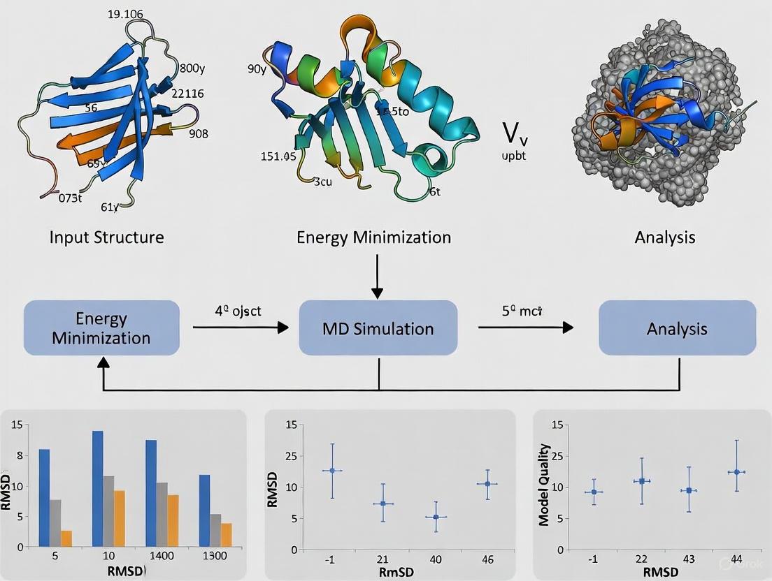
Figure 1: Computational workflow for defining enzyme active site characteristics, integrating both sequence-based and structure-based approaches with quality assessment metrics.
Advanced AI-Driven Approaches for Active Site Analysis
Substrate Specificity Prediction with EZSpecificity
EZSpecificity is a cross-attention-empowered SE(3)-equivariant graph neural network architecture for predicting enzyme substrate specificity, trained on a comprehensive database of enzyme-substrate interactions at sequence and structural levels [2]. This model outperforms existing machine learning approaches for enzyme substrate specificity prediction, achieving 91.7% accuracy in identifying single potential reactive substrates compared to 58.3% for state-of-the-art models in experimental validation with halogenases [2].
Protocol: Substrate Scope Prediction
- Input Preparation: Provide enzyme structure and potential substrates
- Feature Extraction: EZSpecificity generates numerical representations of enzyme active sites and substrates
- Interaction Modeling: The cross-attention mechanism identifies complementary features between enzymes and substrates
- Specificity Scoring: Outputs likelihood scores for enzyme-substrate pairs
- Experimental Validation: Prioritize predicted substrates for testing
AI-Enabled Enzyme Design
Recent breakthroughs in AI-driven protein design now enable the generation of efficient protein catalysts with complex active sites tailored for specific chemical reactions [6]. These approaches integrate deep learning-based protein design with novel assessment tools to evaluate catalytic preorganization across multiple reaction states.
Protocol: De Novo Enzyme Design
- Reaction Definition: Specify target chemical transformation and mechanism
- Active Site Scaffolding: Generate protein folds that position catalytic residues optimally
- Sequence Optimization: Design sequences that stabilize the intended fold and active site geometry
- In Silico Screening: Evaluate designs for structural integrity and catalytic preorganization
- Experimental Characterization: Test designed enzymes for activity and specificity
In one demonstration of this approach, over 300 computer-generated proteins were tested in the lab, with a subset showing reactivity with chemical probes, indicating successful installation of an activated catalytic serine [6]. Structural analysis revealed that the designed enzymes closely matched their intended architectures, with crystal structures deviating by less than 1 Å from computational models [6].
Table 2: Key Research Reagent Solutions for Enzyme Active Site Studies
| Tool/Resource | Type | Primary Function | Application Context |
|---|---|---|---|
| CASA Workflow | Software Package | Automated sequence annotation with custom feature mapping | Identifying conserved active site residues in novel enzymes [4] |
| DeepMolecules | Web Server | Predicting enzyme-substrate pairs and kinetic parameters | Virtual screening of potential substrates; metabolic engineering [3] |
| EZSpecificity | Deep Learning Model | Substrate specificity prediction from enzyme structure | Determining enzyme function and promiscuity [2] |
| GNINA | Docking Software | Molecular docking with CNN-based scoring | Structure-based analysis of ligand binding in active sites [5] |
| EnzyMS | Python Pipeline | LC-MS data analysis for biocatalysis experiments | Detecting enzymatic reaction products and unexpected outcomes [7] |
| RoseTTAFold | AI Protein Design | De novo enzyme design with complex active sites | Creating custom enzymes for specific chemical transformations [6] |
| ZRANK2 | Scoring Function | Ranking protein-protein complex conformations | Assessing macromolecular interactions involving enzymes [8] |
| PyDock | Scoring Function | Electrostatic and desolvation energy-based scoring | Evaluating protein-protein docking in enzyme complexes [8] |
Defining enzyme active sites requires a multi-faceted approach that integrates sequence analysis, structural characterization, and computational modeling. The key structural features—including catalytic triads, metal coordination sites, and specific binding pockets—create unique microenvironments optimized for substrate recognition and transition state stabilization. Functional characterization through kinetic parameters and substrate specificity profiling provides insights into catalytic mechanisms and efficiency.
The protocols outlined here, from sequence annotation with CASA to structure-based analysis with molecular docking and AI-driven design, provide researchers with comprehensive methodologies for active site investigation. Critical to these approaches is the rigorous assessment of model quality through ROC analysis, CNN scoring, and experimental validation. As AI methods continue to advance, the precision with which we can define, predict, and even design enzyme active sites will further accelerate applications in drug discovery, metabolic engineering, and sustainable biotechnology.
Accurate data annotation is a foundational step in developing reliable computational models for biomedical research. It involves the precise labeling of key biological elements—such as enzyme active sites or disease subtypes—to create high-quality datasets that train machine learning (ML) and artificial intelligence (AI) algorithms. The performance of these models is critically dependent on the quality of their underlying annotations; even advanced algorithms can fail or produce misleading results if trained on inconsistent or error-filled data [9] [10]. This application note explores the critical importance of accurate annotation, focusing on its applications in two key areas: the identification of enzyme active sites for drug discovery and the classification of disease subtypes for personalized medicine. We provide detailed protocols and data summaries to guide researchers in implementing these annotation strategies effectively.
The Critical Role of Annotation in Model Performance
In supervised machine learning, models learn patterns from the data they are provided. When this data contains annotation inaccuracies, the model's ability to learn the true underlying patterns is compromised. The principle of "garbage in, garbage out" is particularly relevant here.
Impact on Clinical Decision-Making: A 2023 study highlighted the profound implications of annotation inconsistencies in healthcare. When 11 intensive care unit (ICU) consultants independently annotated the same patient dataset, the resulting inter-annotator agreement was only fair (Fleiss’ κ = 0.383). Classifiers built from these individually annotated datasets subsequently showed low pairwise agreement (average Cohen’s κ = 0.255) when applied to an external validation dataset. This demonstrates that annotation inconsistencies directly propagate into inconsistent model predictions, which in critical care settings can impact patient discharge and mortality decisions [10].
Sources of Annotation Error: Major sources of inconsistency include human subjectivity, data complexity, insufficient domain expertise, and ambiguity in the data itself. For instance, annotating complex medical images or genomic sequences requires specialized knowledge, and a lack of clear guidelines can lead to significant inter-annotator variability [9] [10].
Table 1: Common Challenges in Biological Data Annotation and Their Impacts
| Challenge | Description | Potential Impact on Model |
|---|---|---|
| Human Subjectivity | Variation in interpretation among annotators, especially with nuanced data. | Introduces inconsistent labels, reducing model reliability and accuracy [9]. |
| Data Complexity | Requires specialized expertise (e.g., for medical images or enzyme structures). | Errors from lack of expertise compromise the model's ability to learn true patterns [9]. |
| Ambiguity & Context | Data that can be interpreted in multiple ways depending on context. | Leads to mislabeled data, causing the model to learn incorrect associations [9]. |
| Insufficient Information | Poor quality data or unclear annotation guidelines. | Prevents reliable labeling, resulting in a "shifting ground truth" and unstable models [10]. |
Application Note 1: Accurate Annotation of Enzyme Active Sites in Drug Discovery
Background and Rationale
Enzymes are fundamental catalysts in biochemical processes, and their active sites are primary targets for drug design. Accurately annotating these active sites is crucial for understanding disease mechanisms and developing therapeutic inhibitors. However, high-quality annotation is challenging; of over forty million enzyme sequences identified in the UniProt database, less than 0.7% have high-quality annotations of their active sites [11]. This scarcity of reliable data has historically hindered computational approaches.
Recent advances in AI are overcoming these limitations. The EasIFA (Enzyme active site Identification by Feature Alignment) algorithm exemplifies how multi-modal deep learning can leverage accurate annotations to achieve breakthroughs in speed and precision [11].
Quantitative Performance of Advanced Annotation Tools
The integration of protein language models and 3D structural encoders has led to significant performance improvements.
Table 2: Performance Comparison of Enzyme Active Site Annotation Tools
| Annotation Method | Key Principle | Recall Improvement | Speed Increase | Key Advantage |
|---|---|---|---|---|
| EasIFA (Proposed) | Multi-modal deep learning fusing sequence, structure, and reaction data [11]. | +7.57% vs. BLASTp [11] | 10x faster than BLASTp; 650-1400x faster than PSSM-based DL [11] | High accuracy and speed, suitable for large-scale annotation. |
| BLASTp | Homology-based sequence alignment [11]. | Baseline | Baseline | Well-established, but performance drops if similar sequences are absent from the database. |
| AEGAN | Structure-based graph network using PSSM features [11]. | High accuracy | Baseline (Slow) | Good performance but computationally expensive, limiting large-scale use. |
| 3D Catalytic Modules | Identifies recurring 3D structural motifs in active sites [12]. | Functional insights | Not Specified | Provides mechanistic understanding, useful for enzyme design. |
Experimental Protocol: Annotation of Enzyme Active Sites Using EasIFA
Objective: To accurately annotate catalytic residues in an enzyme's amino acid sequence using its 3D structure and reaction information.
Materials and Reagents:
- Input Data: Enzyme structure file (PDB format) and the chemical reaction it catalyzes (Reaction SMILES format) [11].
- Software: EasIFA algorithm (Freely accessible via web server at http://easifa.iddd.group) [11].
- Computing Environment: Standard computer with internet access for the web server; for local installation, a Python environment with necessary deep learning libraries (e.g., PyTorch) is required.
Procedure:
- Data Preparation:
- Obtain the 3D atomic coordinates of the target enzyme in PDB format. This can be from an experimental source (e.g., RCSB PDB) or a computational prediction (e.g., AlphaFold2).
- Define the enzymatic reaction catalyzed by the target enzyme in SMILES (Simplified Molecular Input Line Entry System) format [11].
Feature Extraction:
- The enzyme's amino acid sequence is processed by a protein language model (e.g., ESM) to extract evolutionary and contextual features.
- The 3D enzyme structure is encoded using a structural encoder to capture spatial relationships and physicochemical properties of residues [11].
- The reaction SMILES is processed by a lightweight graph neural network, pre-trained on a broad dataset of organic reactions, to generate a representation of the chemical transformation [11].
Multi-Modal Information Fusion:
- The latent representations from the protein language model and the 3D structural encoder are fused.
- A multi-modal cross-attention framework aligns the combined enzyme representation with the reaction representation. This step allows the model to focus on enzyme residues that are relevant to the specific chemical reaction being catalyzed [11].
Active Site Prediction:
- The fused and aligned features are fed into a classifier (e.g., a multi-layer perceptron) to generate per-residue predictions.
- The output is a probability score for each amino acid residue in the sequence, indicating its likelihood of being part of the active site. Residues with scores above a defined threshold (e.g., 0.5) are annotated as active site residues [11].
Validation:
- Where possible, compare the predictions with experimentally validated catalytic residues from databases such as the Mechanism and Catalytic Site Atlas (M-CSA) [12].
The following workflow diagram illustrates the streamlined EasIFA annotation process:
The Scientist's Toolkit: Research Reagent Solutions for Enzyme Annotation
Table 3: Essential Resources for Enzyme Active Site Research
| Item/Tool Name | Function/Application | Specifications/Notes |
|---|---|---|
| EasIFA Web Server | Automated annotation of enzyme active sites from structure and reaction data. | Freely available at http://easifa.iddd.group; no local installation required [11]. |
| Mechanism and Catalytic Site Atlas (M-CSA) | Database of enzyme catalytic mechanisms and annotated active sites. | Used for model training and validation; provides expert-curated gold-standard data [12]. |
| 3D Catalytic Template Library | A compiled library of recurring 3D modules in enzyme active sites. | Useful for understanding catalytic function and for enzyme design [12]. |
| AlphaFold2 | Protein structure prediction tool. | Generates reliable 3D structural models when experimental structures are unavailable [11]. |
Application Note 2: Annotation of Disease Subtypes for Personalized Medicine
Background and Rationale
Distinguishing diseases into distinct subtypes is crucial for developing effective, personalized treatment strategies. The Open Targets Platform integrates vast biomedical datasets to support disease classification, yet many disease annotations remain incomplete, requiring laborious expert input [13]. This is especially problematic for rare diseases. Machine learning models trained on accurately annotated datasets can predict disease subtypes from genomic, phenotypic, and clinical data, enabling a more robust and scalable approach to ontology completion [13].
Quantitative Performance in Disease Subtype Identification
A machine learning model designed to identify diseases with potential subtypes achieved a high ROC AUC (Area Under the Receiver Operating Characteristic Curve) of 89.4% [13]. This performance demonstrates the model's strong capability to distinguish between diseases with and without known subtypes. Furthermore, the model identified 515 disease candidates predicted to possess previously unannotated subtypes, offering novel targets for personalized medicine and drug repurposing [13].
Experimental Protocol: Predicting Novel Disease Subtypes
Objective: To build a machine learning model that identifies diseases likely to have unannotated subtypes using features from integrated biomedical datasets.
Materials and Reagents:
- Data Source: The Open Targets Platform (OT), which integrates approximately 23,000 diseases with genetic, genomic, and biochemical data [13].
- Features: Novel features derived from direct evidence, such as genetic associations (from GWAS), phenotypic data (from HPO), and pathway information [13].
- Software: Machine learning libraries (e.g., Scikit-learn for Random Forest/LR) and deep learning frameworks (for integrating pre-trained language models) [13].
Procedure:
- Dataset Curation:
- Extract known disease-subtype relationships from established ontologies like the Experimental Factor Ontology (EFO) and Orphanet to create a labeled training set [13].
- For each disease, compute feature vectors representing genetic, phenotypic, and environmental associations.
Feature Engineering and Model Training:
- Split the data into training and validation sets using cross-validation (CV) to ensure robust performance estimation [13].
- Train multiple classifier models, such as Logistic Regression (LR) and Random Forest (RF). Integrate embeddings from pre-trained deep-learning language models to capture semantic information from biomedical literature [13].
- Use feature importance analysis (e.g., SHAP values) to interpret which data types (genetic, phenotypic, etc.) most strongly contribute to predictions [13].
Prediction and Candidate Prioritization:
- Apply the trained model to all diseases in the Open Targets Platform.
- Diseases with high prediction scores but no current subtype annotations in the database are considered high-confidence candidates for novel subtypes.
- Generate a ranked list of candidate diseases (e.g., the 515 candidates identified) for further experimental validation [13].
The following workflow summarizes the disease subtype prediction process:
Best Practices for High-Quality Data Annotation
To ensure the development of robust AI models, adhering to established annotation best practices is essential.
- Develop Detailed Annotation Guidelines: Create comprehensive documentation with clear label definitions, practical examples of common and edge cases, and instructions for handling ambiguities. This minimizes subjectivity and aligns all annotators [14] [9].
- Implement Rigorous Quality Control: Employ a multi-tiered validation system. This includes peer review, redundant annotations (multiple annotators per data point), and the use of agreement metrics like the Kappa coefficient to measure consistency [9] [10].
- Leverage AI-Assisted Annotation and Active Learning: Use pre-trained models to suggest initial annotations, which human experts can then validate or correct. An active learning approach, where the model prioritizes the most uncertain data for annotation, maximizes efficiency and impact [9].
- Involve Domain Experts: For complex fields like enzymology and medicine, the involvement of biochemists, pathologists, and clinicians is non-negotiable. Their expertise ensures contextual accuracy and handles nuances that non-specialists might miss [9] [10].
Accurate data annotation is not a mere preliminary step but a critical determinant of success in computational biology and drug discovery. As demonstrated, advanced annotation tools like EasIFA for enzyme active sites and ML models for disease subtypes are achieving high performance, enabling large-scale, reliable applications that were previously infeasible. By adhering to the detailed protocols and best practices outlined in this document—such as using multi-modal data, implementing robust quality control, and leveraging domain expertise—researchers can build more accurate and trustworthy models. Ultimately, precise annotation directly accelerates the pace of scientific discovery, from identifying novel drug targets to enabling personalized medicine through refined disease classification.
A profound data challenge lies at the heart of modern enzymology: the critical gap between the linear protein sequences being generated at an unprecedented rate and their detailed functional annotation. While advances in sequencing technology have made enzyme sequences readily available, the experimental characterization of their active sites—the specific regions responsible for catalytic activity—has failed to keep pace. The UniProt database reveals that despite the identification of over forty million enzyme sequences, less than 0.7% have high-quality annotations of their active sites [11]. This massive annotation deficit impedes progress across multiple fields, including drug discovery, disease research, and enzyme engineering, where understanding catalytic mechanisms is paramount.
This application note addresses this challenge by presenting structured protocols and computational solutions for accurate enzyme active site annotation. We frame these methodologies within the broader context of assessing model quality for enzyme active site research, providing researchers with practical tools to bridge the sequence-function divide through integrated computational approaches that leverage both evolutionary and structural information.
Quantitative Landscape of the Annotation Gap
Table 1: Scale of the Enzyme Sequence-Function Annotation Gap
| Metric | Value | Source | Implication |
|---|---|---|---|
| Annotated enzyme sequences in UniProtKB/Swiss-Prot | 216,785 records (38.6% of total) | [15] | Vast majority of sequences lack expert curation |
| Rhea reactions mapped in UniProtKB/Swiss-Prot | 6,654 unique reactions | [15] | Coverage of biochemical transformations remains incomplete |
| Rhea reactions linked to EC numbers | ~75% (4,938 reactions) | [15] | Significant portion of reactions lack standard classification |
| Sequences with high-quality active site annotations | <0.7% | [11] | Critical catalytic information is missing for most enzymes |
Integrated Tools for Active Site Annotation
Table 2: Computational Tools for Enzyme Active Site Annotation
| Tool | Methodology | Input | Output | Strengths |
|---|---|---|---|---|
| EasIFA [11] | Multi-modal deep learning (PLM + 3D structure) | Protein structure, reaction SMILES | Active site residues with types | 10x faster than BLASTp, high accuracy |
| CAPIM [16] | Integrates P2Rank, GASS, and AutoDock Vina | Protein structure | Binding pockets, catalytic residues, EC numbers, docking validation | Residue-level function annotation; multimer support |
| GASS [16] | Genetic algorithm with structural templates | Protein structure | Catalytic residues, EC numbers | Identifies residues across different protein chains |
| P2Rank [16] | Machine learning (Random Forest) | Protein structure | Ligand-binding pockets | Template-free approach; suitable for automation |
Protocol 1: Multi-Modal Active Site Annotation with EasIFA
Application Note: EasIFA (Enzyme active site annotation) represents a significant advancement in annotation technology by fusing protein language models with 3D structural encoders, enabling both rapid and accurate identification of catalytic residues.
Experimental Protocol:
Input Preparation:
- Obtain the protein structure file in PDB format for the enzyme of interest.
- Prepare the corresponding enzymatic reaction information in Reaction SMILES format.
Feature Extraction:
- Process the amino acid sequence through a protein language model (ESM) to generate evolutionary context embeddings.
- Encode the 3D structural information using a graph neural network to capture spatial relationships.
- Utilize a pre-trained molecular transformer to encode the reaction SMILES into a latent representation.
Multi-Modal Fusion:
- Employ a cross-attention mechanism to align the protein-level representations with the reaction knowledge.
- This fusion enables the model to understand the relationship between the enzyme's structure and the specific chemistry it catalyzes.
Active Site Prediction:
- The fused representations are processed through a classification layer to predict whether each amino acid residue belongs to an active site.
- The model further classifies the type of active site (e.g., catalytic vs. binding).
Validation:
- Compare predictions against known annotated structures in databases such as the Catalytic Site Atlas (CSA).
- Performance metrics including recall, precision, F1 score, and Matthews correlation coefficient (MCC) should be calculated to assess model quality.
Figure 1: EasIFA Multi-Modal Annotation Workflow
Protocol 2: Residue-Level Functional Annotation with CAPIM
Application Note: CAPIM addresses the critical gap between catalytic site identification and functional characterization by integrating pocket detection, EC number assignment, and docking validation in a unified pipeline, with particular utility for multimeric enzymes.
Experimental Protocol:
Binding Pocket Prediction:
- Input the protein structure (in PDB format) into P2Rank.
- P2Rank generates solvent-accessible points and uses a Random Forest classifier to evaluate ligandability based on physicochemical and geometric features.
- Output is a ranked list of predicted binding pockets with their spatial coordinates.
Catalytic Residue Identification and EC Number Assignment:
- Process the same protein structure using GASS (Genetic Active Site Search).
- GASS employs genetic algorithms to compare the query structure against a database of active site templates.
- The output includes identification of catalytically active residues and assignment of potential Enzyme Commission (EC) numbers based on template matches.
Data Integration and Analysis:
- Merge P2Rank and GASS outputs to generate residue-level activity profiles within predicted pockets.
- Correlate spatial pocket information with functional EC number annotations.
Functional Validation via Docking:
- Prepare ligand structures of known substrates for the predicted EC classes.
- Use AutoDock Vina to perform docking simulations into the predicted binding pockets.
- Analyze binding poses and affinities to validate the functional predictions.
Quality Assessment:
- For homomeric enzymes, special attention must be paid to symmetric interface accuracy, as inaccurate interface modeling can prevent atomic-level accuracy in active site prediction [17].
- Cross-validate predictions against experimental data where available.
Figure 2: CAPIM Integrated Annotation Pipeline
The Scientist's Toolkit: Research Reagent Solutions
Table 3: Essential Databases and Resources for Enzyme Annotation
| Resource | Type | Function | Application in Annotation |
|---|---|---|---|
| RCSB PDB Annotations [18] | Database | Aggregates structural domain and gene ontology information | Provides evolutionary context (CATH, SCOP) and functional clues (GO terms) |
| Rhea [15] | Biochemical reaction knowledgebase | Expert-curated biochemical reactions with ChEBI ontology | Standardized enzyme annotation in UniProtKB; connects sequences to chemistry |
| Catalytic Site Atlas (CSA) | Database | Manually curated catalytic residues in enzyme structures | Gold-standard validation set for predictive tools |
| UniProtKB [15] | Protein sequence database | Central repository of protein sequence and functional information | Primary source of sequence data with Rhea-integrated enzyme annotation |
| EC Number Classification | Nomenclature system | Hierarchical classification of enzymes by catalyzed reaction | Standardized functional classification across tools and databases |
The integration of multi-modal computational approaches represents a paradigm shift in addressing the enzyme annotation challenge. By simultaneously leveraging sequence embeddings, structural information, and chemical reaction data, tools like EasIFA and CAPIM demonstrate that it is possible to achieve both high accuracy and efficiency in active site prediction. The protocols outlined in this application note provide researchers with standardized methodologies for implementing these advanced annotation strategies, creating a foundation for more reliable assessment of model quality in enzyme active site research. As these computational methods continue to evolve, they will dramatically accelerate our ability to translate the vast landscape of enzyme sequences into functional understanding, ultimately driving innovation across biotechnology, drug discovery, and fundamental biochemical research.
The accurate prediction of protein structure, particularly for enzyme active sites, is a cornerstone of modern drug discovery and biotechnology. The evolution of computational methods from traditional homology modeling to contemporary artificial intelligence (AI) has fundamentally transformed this field, enabling unprecedented accuracy in modeling functional sites. This progression represents a paradigm shift from reliance on evolutionary templates to the de novo generation of structures through deep learning. Within enzyme research, where function is dictated by the precise three-dimensional geometry of active sites, this evolution is critically important for assessing the quality and reliability of structural models. The journey began with homology modeling, which depended on structural similarities with known proteins, and has now reached a new era with AI systems like AlphaFold achieving atomic accuracy, thereby offering profound implications for understanding enzyme mechanism and function [19] [20].
The Foundation: Homology Modeling
Homology modeling, also known as comparative modeling, established the foundational framework for computational protein structure prediction. This methodology is predicated on two core principles: that a protein's amino acid sequence determines its three-dimensional structure, and that this structure is more conserved than its sequence over evolutionary time. When a protein of unknown structure (the target) shares a detectable level of sequence similarity with one or more proteins of known structure (the templates), the structural coordinates of the templates can be used to model the target [20].
The classical homology modeling process is a sequential pipeline involving multiple, refined steps:
- Template Identification and Selection: The target sequence is searched against protein structure databases like the Protein Data Bank (PDB) using tools such as BLASTp, HHblits, or JackHMMER to identify suitable templates.
- Alignment Correction and Optimization: The sequence alignment between the target and template(s) is carefully optimized to minimize errors from gaps and mutations, often using multiple sequence alignments from tools like CLUSTALW or MUSCLE.
- Backbone Model Building: The backbone of the target protein is constructed based on the coordinates of the aligned regions in the template. This can be achieved through rigid-body assembly, segment matching, or spatial restraint methods.
- Loop Modeling and Side-Chain Addition: Regions not aligned with any template, typically loops, are modeled separately. Side-chain conformations (rotamers) are then built onto the backbone.
- Model Optimization and Validation: The initial model is subjected to energy minimization and molecular dynamics to relieve steric clashes and improve stereochemistry. The final model is validated using geometric checks and statistical potentials [20].
A significant challenge for homology modeling, particularly in the context of enzyme active sites, has been the accurate prediction of binding site residues from sequence alone. To address this, evolutionary approaches were developed that leverage the principle that spatial patterns of functional residues are conserved. One such method constructed a database of pocket-containing segments and used a residue-matching profiling technique to predict binding site residues with a reported precision of 70% at 60% sensitivity, even when sequence identity with the template was below 30% [21].
Table 1: Key Steps in the Homology Modeling Pipeline
| Step | Key Methods/Tools | Primary Objective | Challenge for Active Sites |
|---|---|---|---|
| 1. Template Identification | BLASTp, psi-BLAST, HHblits, JackHMMER | Find structurally characterized homologs | Low sequence identity can lead to misalignment of functional residues. |
| 2. Alignment Optimization | CLUSTALW, MUSCLE, profile-profile alignment | Maximize alignment accuracy for core regions | Gaps and shifts can distort the geometry of the binding pocket. |
| 3. Backbone Construction | MODELLER, SWISS-MODEL | Build a initial 3D coordinate set | Conserved backbone geometry may not reflect catalytic state. |
| 4. Loop & Side-Chain Modeling | Ab initio loop modeling, rotamer libraries | Model variable regions and atomic details | High flexibility of catalytic loops is difficult to sample accurately. |
| 5. Validation | MolProbity, PROCHECK, Verify3D | Assess structural reasonableness | Physics-based force fields may not correctly rank models for function. |
For enzyme active site research, the primary limitation of homology modeling is its inherent dependence on the existence and quality of available templates. If the template's active site is not representative of the target's true catalytic state, or if the target possesses a novel fold, the model will be unreliable. Furthermore, the method often fails to capture the dynamic reality of proteins in their native biological environments, a critical aspect for understanding enzyme mechanism [22].
The AI Revolution in Structure Prediction
The advent of artificial intelligence has catalyzed a revolutionary shift in protein structure prediction, moving beyond the template constraints of homology modeling to achieve unprecedented atomic-level accuracy. This revolution is exemplified by DeepMind's AlphaFold2, which demonstrated in the 14th Critical Assessment of protein Structure Prediction (CASP14) that computational methods could regularly predict protein structures to near-experimental accuracy [19]. The core innovation of modern AI systems lies in their ability to learn the complex relationships between protein sequence, evolutionary history, and 3D structure directly from vast datasets of known sequences and structures.
AlphaFold2 introduced several groundbreaking architectural components. Its neural network employs an Evoformer block, a novel architecture that processes input data as a graph inference problem. The Evoformer jointly embeds and refines two key representations: a multiple sequence alignment (MSA) representation and a pair representation that encapsulates relationships between residues. This is followed by a structure module that introduces an explicit 3D structure, iteratively refining it using a novel equivariant transformer to produce accurate coordinates for all heavy atoms [19]. The system incorporates physical and biological knowledge about protein structure and leverages intermediate losses and iterative refinement (recycling) to progressively enhance the predicted model.
The quantitative leap in accuracy has been profound. In CASP14, AlphaFold2 achieved a median backbone accuracy (Cα root-mean-square deviation) of 0.96 Å, a value comparable to the width of a carbon atom and significantly superior to the next best method at 2.8 Å [19]. This level of precision extends to side-chain placement and the packing of domains in large, multi-domain proteins, making these predictions highly useful for inferring enzyme function.
However, AI-based structure prediction faces its own set of challenges. A fundamental epistemological challenge is that the machine learning methods are trained on experimentally determined structures from databases, which may not fully represent the thermodynamic environment controlling protein conformation at functional sites [22]. Furthermore, these methods typically produce single, static models, which are inadequate for representing the millions of possible conformations that proteins—especially those with flexible regions or intrinsic disorders—can adopt in solution. For enzyme active sites, which often rely on precise dynamics for catalysis, this static representation is a significant limitation [22].
Table 2: Evolution of Key Prediction Methods and Their Performance
| Method Era | Representative Tool | Core Methodology | Reported Accuracy (Backbone) | Key Limitation for Active Sites |
|---|---|---|---|---|
| Homology Modeling | MODELLER, SWISS-MODEL | Template-based coordinate assembly | Highly variable; degrades sharply with <30% sequence identity to template. | Template dependence; poor performance on novel folds or binding sites. |
| Deep Learning (c. 2020) | AlphaFold2 [19] | Evoformer & SE(3)-equivariant transformer | 0.96 Å median RMSD (CASP14) | Static structure output; limited representation of dynamics and flexibility. |
| Specificity Prediction | EZSpecificity [2] | SE(3)-equivariant graph neural network | 91.7% accuracy in identifying reactive substrate (vs. 58.3% for previous model) | Focused on substrate specificity, not full atomic structure. |
Application Notes for Enzyme Active Site Research
The transition to AI-driven models has necessitated new protocols for assessing the quality of predicted enzyme active sites. The following application notes provide a structured framework for researchers to validate and utilize these models effectively.
Protocol for Benchmarking Compound Activity Predictions
For drug discovery applications, benchmarking the predictive power of models against real-world experimental data is crucial. The CARA (Compound Activity benchmark for Real-world Applications) benchmark provides a robust framework for this task, distinguishing between two primary application scenarios: Virtual Screening (VS) and Lead Optimization (LO) [23].
Procedure:
- Data Curation and Assay Classification: Collect compound activity data from public resources like ChEMBL, grouped by Assay ID. Classify each assay as either VS-type (characterized by a diverse set of compound scaffolds) or LO-type (characterized by series of congeneric compounds with high similarity).
- Data Splitting: Implement different data splitting schemes tailored to the task.
- For VS tasks, apply a protein-level split, where all data for a specific target protein is held out in the test set. This evaluates the model's ability to generalize to novel targets.
- For LO tasks, apply a scaffold-level split, where compounds sharing a core molecular scaffold are held out. This tests the model's ability to predict activity for novel chemotypes within the same target project.
- Model Training and Evaluation:
- Train selected machine learning or deep learning models (e.g., graph neural networks, random forests) on the training split.
- Evaluate model performance on the test set using metrics appropriate for each task. For VS, prioritize metrics like AUC-ROC and enrichment factors. For LO, use metrics sensitive to ranking quality, such as Spearman's correlation or Kendall's Tau, to assess structure-activity relationships.
Interpretation and Analysis: This protocol helps identify whether a model is fit for a specific purpose in the drug discovery pipeline. It has been observed that popular training strategies like meta-learning can improve performance for VS tasks, while training separate QSAR models per assay can be effective for LO tasks due to their distinct data distributions [23]. This benchmark is essential for avoiding over-optimism and ensuring model utility in practical enzyme inhibitor discovery.
Protocol for Predicting Enzyme Substrate Specificity
Accurately defining an enzyme's function requires predicting its substrate specificity, which originates from the 3D structure of its active site and the complicated reaction transition state. AI models like EZSpecificity have been developed specifically for this task [2].
Procedure:
- Input Data Preparation:
- Sequence & Structure: Obtain the enzyme's amino acid sequence and its 3D structure (either experimentally determined or computationally predicted, e.g., by AlphaFold2).
- Substrate Library: Prepare a library of candidate substrate molecules in a standardized molecular format (e.g., SMILES strings).
- Model Application:
- Input the enzyme and substrate data into the EZSpecificity model. This model uses a cross-attention-empowered SE(3)-equivariant graph neural network architecture, which is inherently aware of 3D rotational and translational symmetries, making it ideal for structural data.
- The model will output a score or probability representing the likelihood of a catalytic reaction between the enzyme and each substrate.
- Validation:
- For high-priority predictions, experimental validation is essential. For example, in the case of halogenases, the top predicted reactive substrate can be tested in vitro, where EZSpecificity achieved an accuracy of 91.7% in identifying the single potential reactive substrate [2].
Key Considerations: This protocol moves beyond static structure prediction to infer dynamic function. The high accuracy of specialized models like EZSpecificity demonstrates how AI can leverage structural information to provide deep functional insights, bridging a critical gap in enzyme characterization.
Protocol for Assessing Model Quality and Dynamics
Given the limitations of static AI models, a critical protocol involves assessing the quality of a predicted active site and inferring its dynamic properties.
Procedure:
- Confidence Metric Analysis: Always examine the per-residue confidence score provided with the prediction (e.g., AlphaFold's pLDDT). Low confidence (typically pLDDT < 70) in active site regions is a major red flag and suggests the model may be unreliable for that locale. The pLDDT score has been shown to reliably predict the local accuracy of the model [19].
- Ensemble Generation: To probe flexibility, use the predicted aligned error (PAE) matrix from models like AlphaFold. A high PAE between the active site and other structural elements suggests potential flexibility or domain movements. Alternatively, use molecular dynamics simulations starting from the AI-predicted structure to sample conformational space.
- Functional Consistency Check: Map known catalytic residues from sequence annotations onto the predicted structure. Verify that the geometric arrangement (distances, angles) between these residues is chemically plausible for the proposed enzymatic mechanism. For proteins with no annotation, tools for functional site prediction can be used.
Interpretation and Analysis: This quality assessment is vital for determining whether a model is sufficient for downstream tasks like drug docking or rational design. A high-confidence, geometrically plausible active site model can be used with high confidence. A low-confidence model necessitates experimental structure determination or the use of more advanced sampling methods to explore conformational ensembles, as single static models cannot represent the dynamic reality of functional proteins [22].
Table 3: Key Software and Database Resources for Enzyme Structure Prediction
| Resource Name | Type | Primary Function in Enzyme Research | Access |
|---|---|---|---|
| AlphaFold [19] | AI Structure Prediction | Predicts 3D protein structure from sequence with high accuracy; provides confidence metrics (pLDDT/PAE). | AlphaFold Protein Structure Database (pre-computed); source code (local deployment). |
| Rosetta [24] | Software Suite | Enables de novo protein design, enzyme engineering, ligand docking, and loop modeling using physics-based and knowledge-based methods. | Rosetta Commons (academic license). |
| EZSpecificity [2] | Specificity Prediction | Predicts enzyme substrate specificity using 3D structural information via a graph neural network. | Code available on Zenodo. |
| ChEMBL [23] | Database | A manually curated database of bioactive molecules with drug-like properties. Used for benchmarking compound activity. | Publicly available online. |
| SplitPocket/PSD [21] | Database (Template Library) | Database of functional pockets and pocket-containing sequence segments; used for template-based binding site prediction. | Publicly available. |
| CARA Benchmark [23] | Benchmarking Dataset | A curated benchmark for evaluating compound activity prediction methods in real-world virtual screening and lead optimization tasks. | Derived from public data. |
Workflow and Relationship Visualizations
Homology to AI Modeling Evolution
Modeling Evolution Workflow
Active Site Quality Assessment
Active Site Quality Check
Cutting-Edge Computational Methods for Active Site Prediction
Application Notes
The integration of protein language models (PLMs) with 3D structural data is revolutionizing computational biology, particularly in the high-precision task of enzyme active site research. This multi-modal approach overcomes the inherent limitations of sequence-only or structure-only models by creating a unified representation that captures evolutionary, structural, and functional constraints. The assessment of model quality in this domain hinges on the ability to accurately annotate catalytic residues and predict functional dynamics, which are critical for drug discovery and enzyme engineering.
Advanced Multi-Modal Architectures for Active Site Analysis
1.1.1. EasIFA: Fusing Sequence, Structure, and Reaction Information The EasIFA (Enzyme active site annotation) framework demonstrates the power of integrating latent enzyme representations from a PLM with 3D structural encoders. Its core innovation lies in a multi-modal cross-attention framework that aligns protein-level information with knowledge of enzymatic reactions. This architecture allows the model to precisely understand the relationship between an enzyme and its specific substrates and reaction types. Evaluated against standard tools, EasIFA outperforms BLASTp with a 10-fold speed increase and improvements in recall (7.57%), precision (13.08%), F1 score (9.68%), and Matthews Correlation Coefficient (0.1012). It also surpasses other deep learning methods based on Position-Specific Scoring Matrices (PSSM), achieving a 650 to 1400-fold speed increase while enhancing annotation quality. This makes it suitable for large-scale industrial and academic applications [11].
1.1.2. OneProt: A Multi-Modal Foundation Model OneProt represents a significant step towards general-purpose multi-modal protein foundation models. It integrates five distinct modalities: protein sequence, 3D structure (in two representations), text annotations, and crucially, binding site data. Using the ImageBind framework, OneProt aligns the latent spaces of these modalities through lightweight fine-tuning that focuses on pairwise alignment with sequence data. This approach enables emergent alignment, where modalities not directly paired during training (e.g., text and binding sites) become aligned through their common connection to the sequence anchor. The model employs a mix of Graph Neural Networks and transformer architectures, with exhaustive ablation studies highlighting the critical contribution of the binding site encoder to its performance on enzyme function prediction and binding site analysis tasks [25].
1.1.3. MICA: Combining Experimental and Predicted Structures For protein structure determination, MICA (Multimodal Integration of Cryo-EM and AlphaFold) exemplifies deep learning integration at both input and output levels. It combines experimental cryo-electron microscopy (cryo-EM) density maps with AlphaFold3-predicted structures using an encoder-decoder architecture with a Feature Pyramid Network (FPN). This allows the model to compensate for limitations in either modality—such as low-resolution regions in cryo-EM maps or incorrectly predicted regions in AF3 structures. Tested on density maps with resolutions between 1.5 Å and 4 Å, MICA significantly outperformed state-of-the-art methods, constructing high-accuracy structural models with an average TM-score of 0.93. This demonstrates the robustness of multi-modal integration for real-world, automated protein structure determination [26].
Quantitative Performance of Multi-Modal Models
Table 1: Performance Metrics of Multi-Modal Models in Key Tasks
| Model Name | Primary Task | Key Metric | Performance | Baseline Comparison |
|---|---|---|---|---|
| EasIFA [11] | Enzyme active site annotation | F1 Score / MCC | Improved by 9.68% / 0.1012 | Outperforms BLASTp & PSSM-based DL |
| EasIFA [11] | Inference Speed | Speed Increase | 10x faster than BLASTp; 650-1400x faster than PSSM-DL | Enables large-scale application |
| MICA [26] | Protein structure modeling | TM-score (Avg.) | 0.93 on high-res cryo-EM maps | Outperforms ModelAngelo & EModelX(+AF) |
| OneProt [25] | Multi-modal retrieval | Downstream Task Accuracy | Enhanced by binding site modality | Ablation shows pocket encoder is crucial |
Table 2: Key Research Reagents and Computational Tools for Multi-Modal Protein Research
| Item Name | Type | Function in Research | Relevant Model/Study |
|---|---|---|---|
| ESM Protein Language Model [11] | Software / Encoder | Provides evolutionary and semantic information from protein sequences. | EasIFA, OneProt |
| AlphaFold3 (AF3) [26] | Software / Encoder | Generates highly accurate 3D structural predictions from amino acid sequences. | MICA |
| Cryo-EM Density Maps [26] | Experimental Data | Provides experimental 3D structural information from cryo-electron microscopy. | MICA |
| Mechanism and Catalytic Site Atlas (M-CSA) [12] | Database | A curated repository of enzyme catalytic mechanisms and active site annotations for training and validation. | 3D Module Library Study |
| Catalytic Site Atlas (CSA) [27] | Database | The largest catalogue of catalytic residues, used for compiling datasets of active site groups. | Active Site Flexibility Study |
| CLoSA Algorithm [27] | Software | A Constraint-based Local Structure Alignment tool for comparing active site geometries and measuring flexibility. | Active Site Flexibility Study |
| Graph Neural Network (GNN) [25] [28] | Software / Architecture | Models protein structures as graphs to capture spatial relationships and residue interactions. | OneProt, STAG-LLM |
| Reaction SMILES [11] | Data Format | Represents the chemical reaction an enzyme catalyzes as a string, providing critical functional context. | EasIFA |
Experimental Protocols
Protocol 1: Multi-Modal Training for Enzyme Active Site Annotation with EasIFA
This protocol outlines the procedure for training a model to annotate enzyme active sites by integrating protein sequence, structure, and reaction information, as exemplified by EasIFA [11].
2.1.1. Input Data Preparation
- Protein Structural Information: Obtain or predict the 3D structure of the target enzyme. If an experimental structure is unavailable from the PDB, use a predictive tool like AlphaFold2. Structure files should be in PDB format.
- Chemical Reaction Information: For the enzyme of interest, retrieve the Reaction SMILES string representing the specific biochemical transformation it catalyzes from a database like Rhea or BRENDA.
- Active Site Annotations: Source high-quality, curated catalytic residue labels from databases like the Mechanism and Catalytic Site Atlas (M-CSA) or Catalytic Site Atlas (CSA) for supervised training.
2.1.2. Feature Extraction and Fusion
- Sequence-Structure Representation:
- Process the amino acid sequence using a pre-trained Protein Language Model (e.g., ESM) to generate a latent representation that captures evolutionary constraints.
- Simultaneously, process the 3D atomic coordinates of the enzyme structure using a 3D structural encoder (e.g., a Graph Neural Network that represents residues as nodes and spatial relationships as edges).
- Fuse the latent representations from the PLM and the structural encoder into a unified enzyme representation.
- Reaction Representation:
- Process the Reaction SMILES string using a lightweight, self-supervised graph neural network pre-trained on a broad dataset of organic chemical reactions. This network should employ an atom-wise, distance-aware attention mechanism.
- Multi-Modal Cross-Attention:
- Design an interpretable, attention-based information interaction network. This network uses cross-attention layers to allow the unified enzyme representation and the reaction representation to interact, enabling the model to focus on protein regions most relevant to the catalytic chemistry.
2.1.3. Model Training and Output
- Task Formulation: Frame the problem as a token classification task, where the model predicts whether each amino acid residue in the sequence is part of the active site.
- Loss Function: Use a standard cross-entropy loss for the classification task between the predicted and true catalytic residue labels.
- Output: The model produces a probability for each residue, indicating its likelihood of being a catalytic residue. A threshold can then be applied to generate the final binary annotation.
The following workflow diagram illustrates the complete EasIFA process:
Protocol 2: Multi-Modal Protein Representation Alignment with OneProt
This protocol describes the method for aligning multiple protein modalities into a shared latent space using a framework like OneProt, which is foundational for many downstream tasks such as retrieval and function prediction [25].
2.2.1. Data Curation and Pairing
- Modalities: Collect data for a set of proteins across the following modalities: Sequence (
ℱ), Structure (𝒮), Text (𝒯), and Binding Site/Pocket (𝒫). - Pairing: Form paired samples
(ai, bi)whereaiis always a protein sequence, andbiis data from one of the other modalities for the same protein. For example:(Sequence_A, Structure_A),(Sequence_A, Text_A),(Sequence_A, Pocket_A). - Pre-processing: To reduce redundancy, cluster the protein sequences at a threshold (e.g., ≤50% identity).
2.2.2. Encoder and Projection Setup
- Modality-Specific Encoders: Utilize pre-trained or train-from-scratch encoders for each modality:
ϕ_ℱ: A transformer-based encoder for protein sequences.ϕ_𝒮: A Graph Neural Network for 3D structures.ϕ_𝒯: A text encoder (e.g., based on BERT) for textual descriptions.ϕ_𝒫: A specialized encoder for binding site pockets.
- Projection Heads: For each encoder, attach a lightweight Multi-Layer Perceptron (MLP) projection head (
proj_ℱ,proj_𝒮, etc.). The purpose of these heads is to map the encoder-specific output vectors into a shared latent space of the same dimensionl.
2.2.3. Contrastive Alignment Training
- Batch Construction: For a batch of size
n, construct batches of paired modalities, always using the sequence as the anchor. For instance, a batch could consist ofn(Sequence, Structure)pairs. - Embedding Calculation:
- For a batch of pairs
{(a1, b1), ..., (an, bn)}, passaiandbithrough their respective encoders and projection heads to get normalized unit embeddings𝐚_iand𝐛_i.
- For a batch of pairs
- Loss Calculation:
- Compute the symmetric InfoNCE (NT-Xent) loss. The loss for a single direction is:
L_ℱ,ℰ = -1/n ∑_i log( exp(𝐚_i^⊤ 𝐛_i / τ) / [ exp(𝐚_i^⊤ 𝐛_i / τ) + ∑_{j≠i} exp(𝐚_i^⊤ 𝐛_j / τ) ] )whereτis a temperature parameter. - The total loss for the batch is the sum of the loss in both directions:
L_total = L_ℱ,ℰ + L_ℰ,ℱ.
- Compute the symmetric InfoNCE (NT-Xent) loss. The loss for a single direction is:
- Sequential Update: Perform a gradient update for the encoders and projection heads of the two modalities in the current pair before moving to the next modality pair in the training step. This sequential optimization aligns all modalities to the sequence anchor.
The following diagram visualizes the representation alignment process:
Protocol 3: Integrating Cryo-EM and AlphaFold3 with MICA for Structure Modeling
This protocol details the multi-modal integration of experimental density maps and AI-predicted structures for building high-accuracy atomic models, as implemented in MICA [26].
2.3.1. Input Data Preprocessing
- Cryo-EM Density Maps: Obtain the cryo-EM density map file for the target protein complex. Preprocess the map to normalize voxel intensities and adjust the grid orientation as needed.
- AlphaFold3 Prediction: Run AlphaFold3 using the amino acid sequences of all protein chains in the complex. This will generate predicted structures and confidence metrics (pLDDT) for each residue.
2.3.2. Multi-Task Deep Learning with Feature Pyramid Network (FPN)
- 3D Grid Feature Extraction: Convert both the cryo-EM density map and the AlphaFold3-predicted structure into 3D voxel grids. Extract feature representations from both grids.
- Encoder-Stack and FPN:
- Pass the fused feature input through a progressive encoder stack comprising three encoder blocks with increasing feature depth to generate hierarchical feature representations.
- Process the encoder output with a Feature Pyramid Network (FPN) to generate multi-scale feature maps. These maps capture hierarchical structural information at different resolutions, from local atomic details to global protein fold patterns.
- Task-Specific Decoding: The FPN feature maps are fed into three separate, hierarchically organized decoder blocks:
- Backbone Atom Decoder: Uses the FPN features to predict the positions of backbone atoms (N, Cα, C, O).
- Cα Atom Decoder: Uses both the FPN features and the predictions from the backbone atom decoder to specifically refine Cα atom positions.
- Amino Acid Decoder: Uses the FPN features and the predictions from both the backbone and Cα decoders to predict the amino acid type at each Cα position.
2.3.3. Backbone Tracing and Refinement
- Initial Backbone Tracing: Use the predicted Cα atoms and their assigned amino acid types to build an initial backbone model. This involves linking Cα positions into chains and registering the sequence.
- Gap Filling and Hybrid Refinement:
- Identify any unmodeled gaps in the initial backbone model.
- Fill these gaps using a sequence-guided Cα extension procedure that leverages the structural information from the corresponding regions of the AlphaFold3-predicted structure.
- Full-Atom Model Building and Refinement:
- Convert the Cα backbone model into a full-atom model using a tool like PULCHRA.
- Finally, refine the full model against the experimental cryo-EM density map using a tool like
phenix.real_space_refineto improve the fit and stereochemical quality.
The workflow for this multi-modal structure determination is as follows:
The accurate annotation of enzyme active sites is a cornerstone for advancing drug discovery, disease research, and enzyme engineering. However, a significant trade-off between speed and accuracy has long hindered the large-scale application of automated annotation tools. The EasIFA (enzyme active site annotation algorithm) framework addresses this challenge by introducing a multi-modal deep learning approach that fuses latent enzyme representations from a Protein Language Model (PLM) and a 3D structural encoder. A key innovation is its use of a multi-modal cross-attention framework to align protein-level information with the knowledge of enzymatic reactions. This architecture enables EasIFA to outperform traditional homology-based methods like BLASTp by a substantial margin, achieving not only superior accuracy but also a 10-fold increase in inference speed. Furthermore, it surpasses other state-of-the-art deep learning methods, providing a speed increase of 650 to 1400 times while simultaneously enhancing annotation quality, making it a suitable replacement for conventional tools in both industrial and academic settings [11] [29].
Performance Benchmarking and Quantitative Assessment
To assess the quality of a model for enzyme active site research, it is crucial to evaluate its performance against established benchmarks. The following tables summarize the key quantitative metrics demonstrating EasIFA's capabilities compared to other methods.
Table 1: Performance Comparison of EasIFA Against BLASTp and AEGAN on Key Metrics [11]
| Model | Recall (%) | Precision (%) | F1 Score | MCC | Relative Speed |
|---|---|---|---|---|---|
| EasIFA | +7.57 | +13.08 | +9.68 | +0.1012 | 10x faster |
| BLASTp (Baseline) | Baseline | Baseline | Baseline | Baseline | 1x |
| EasIFA | - | - | - | - | ~1400x faster |
| AEGAN (PSSM-based) | - | - | - | - | 1x |
MCC: Matthews Correlation Coefficient
Table 2: Overview of Modern Enzyme Active Site Prediction Tools
| Tool Name | Modality | Key Innovation | Primary Application |
|---|---|---|---|
| EasIFA [11] | Sequence, Structure, Reaction | Multi-modal cross-attention between enzyme and reaction data | High-speed, accurate active site annotation |
| Squidly [30] | Sequence-only | Biology-informed contrastive learning on PLM embeddings | Fast, large-scale screening from sequence alone |
| OmniESI [31] | Enzyme-Substrate Interaction | Two-stage progressive conditional deep learning | Multi-task prediction (kinetics, pairing, mutation, annotation) |
| EZSpecificity [2] | Structure, Sequence | Cross-attention SE(3)-equivariant GNN | Predicting enzyme substrate specificity |
Experimental Protocols for Model Evaluation
For researchers to independently verify the performance claims of EasIFA and similar models, the following detailed methodologies are provided for key benchmarking experiments.
Protocol for Benchmarking Against BLASTp and Structure-Based Tools
Objective: To compare the annotation accuracy and inference speed of EasIFA against BLASTp and empirical-rule-based algorithms (e.g., SiteMap) [11].
Materials:
- Test Dataset: A standardized benchmark dataset such as CataloDB [30] or others derived from UniProt and M-CSA (Mechanism and Catalytic Site Atlas) with experimentally validated active sites.
- Hardware: A computing node with a modern GPU (e.g., NVIDIA V100 or A100) for deep learning models and standard CPU resources for BLASTp.
- Software: EasIFA (available via its web server http://easifa.iddd.group), BLASTp suite, and Schrödinger's SiteMap.
Procedure:
- Data Preparation: Curate a test set of enzyme sequences and their corresponding 3D structures (from PDB or predicted via AlphaFold2). Ensure the dataset includes the associated reaction SMILES strings for EasIFA.
- Run BLASTp:
- Use the query enzyme sequence as input against a comprehensive protein database (e.g., Swiss-Prot).
- Execute BLASTp with standard parameters, recording the runtime.
- Extract active site annotations from the top homologous hits.
- Run Empirical-Rule-Based Tool (e.g., SiteMap):
- Input the 3D structure of the enzyme.
- Execute the software's binding site detection function.
- Record the predicted catalytic pockets and the computation time.
- Run EasIFA:
- Input the enzyme's 3D structure (PDB format) and its chemical reaction sequence (SMILES format).
- Execute the EasIFA model.
- Record the predicted active site residues and the inference time.
- Evaluation:
- Calculate recall, precision, F1 score, and MCC using the experimentally validated active sites as the ground truth.
- Compare the computational time of each method, normalizing to the slowest method for relative speed calculation.
Protocol for Low-Sequence-Identity Generalization Test
Objective: To evaluate the model's performance on enzymes with low homology to those in the training set, assessing its generalizability [30].
Materials:
- Test Dataset: A specialized benchmark like CataloDB, which is explicitly designed to contain test sequences with less than 30% sequence and structural identity to the training set [30].
- Software: EasIFA and other models for comparison (e.g., Squidly, AEGAN).
Procedure:
- Dataset Splitting: Use the predefined training and test splits of the benchmark dataset to ensure no data leakage.
- Model Inference: Run the trained models on the low-identity test set.
- Performance Analysis: Calculate the F1 score and other metrics specifically on this challenging subset. A model that maintains a high F1 score (e.g., Squidly reports 0.64 on <30% identity sequences [30]) demonstrates robust generalization.
Workflow and Architecture Visualization
Diagram 1: EasIFA Multi-modal Annotation Workflow. The framework integrates representations from three distinct modalities (sequence, structure, and reaction) via a cross-attention mechanism to produce final active site annotations [11].
Successful application and development of enzyme annotation models require a suite of computational tools and data resources.
Table 3: Key Research Reagent Solutions for Enzyme Active Site Research
| Resource | Type | Function & Application | Access |
|---|---|---|---|
| ESM-2 [11] [30] | Protein Language Model | Generates high-quality, biologically meaningful representations from amino acid sequences alone. | Publicly Available |
| AlphaFold2 [11] [32] | Structure Prediction | Provides reliable 3D structural models for enzymes where experimental structures are unavailable. | Publicly Available |
| UniProt [11] [30] | Protein Database | Source of enzyme sequences and high-quality, manually curated active site annotations for training and testing. | Publicly Available |
| M-CSA [30] | Mechanism Database | A manually curated database of enzyme catalytic mechanisms and active sites; essential for creating high-quality benchmark sets. | Publicly Available |
| CataloDB [30] | Benchmark Dataset | A modern benchmark designed to evaluate model performance on low-sequence-identity enzymes, reducing evaluation bias. | Research Paper |
| EasIFA Web Server [11] | Annotation Tool | A user-friendly web interface for running the EasIFA algorithm without local installation. | http://easifa.iddd.group |
Homology modeling, a cornerstone of structural bioinformatics, predicts a protein's three-dimensional structure based on its sequence similarity to templates with experimentally determined structures. While traditional methods have relied heavily on sequence alignment accuracy, the integration of geometric constraints has emerged as a transformative approach for enhancing atomic-level accuracy, particularly in functionally critical regions like enzyme active sites. These constraints, derived from physical laws, evolutionary conservation, and machine learning predictions, restrict the conformational search space to biologically plausible configurations, leading to more reliable models. This application note details protocols for incorporating geometric constraints into homology modeling workflows, with a specific focus on improving the model quality for enzyme active site research, which is essential for accurate function annotation and drug discovery.
The Performance of Geometric Constraint-Based Refinement
Integrating geometric constraints into protein structure prediction and refinement significantly improves model accuracy across diverse protein classes. The following table summarizes the performance gains reported by various constraint-based methodologies.
Table 1: Performance Metrics of Geometric Constraint-Based Modeling Approaches
| Method / Tool | Core Approach | Key Performance Metric | Reported Improvement | Application Focus |
|---|---|---|---|---|
| GraphEC [33] | Geometric graph learning on ESMFold structures | AUC for active site prediction | 0.9583 on independent test set TS124 [33] | Enzyme active site & EC number prediction |
| Constraint-Guided Beta-Sheet Refinement [34] | Local search with residue-distance scores & geometric restrictions | Average RMSD, TM-score, GDT | >12% improvement in average RMSD vs. state-of-the-art methods [34] | Beta-sheet structure refinement |
| ZAM with FRODA & r-REMD [35] | Geometric simulation (FRODA) with physics-based refinement (r-REMD) | RMSD from native structure | Reduced from 3.7 Å to 2.7 Å after refinement [35] | De novo structure prediction for α-, β-, α/β-proteins |
| AlphaFold2 [19] | End-to-end deep learning with physical/geometric constraints | Median backbone accuracy (Cα r.m.s.d.95) | 0.96 Å, vastly outperforming other methods [19] | General protein structure prediction |
The quantitative data demonstrates that methods leveraging geometric information consistently yield higher accuracy. For instance, GraphEC's high AUC score underscores the power of combining predicted structures with geometric learning for identifying functionally critical residues [33]. Furthermore, the refinement of initially assembled structures using physics-based molecular dynamics, as in the ZAMF method, leads to a substantial reduction in RMSD, highlighting the importance of a multi-stage approach that combines coarse geometric sampling with detailed atomic-level refinement [35].
Protocols for Integrating Geometric Constraints
This section provides detailed methodologies for implementing geometric constraint-guided modeling, from initial template selection to final model validation.
Protocol 1: Template Selection and Structure Preparation
Objective: To identify suitable homology modeling templates and prepare initial structures with a focus on active site geometry.
Identify Catalytic Modules:
- Action: Prior to template search, query the Mechanism and Catalytic Site Atlas (M-CSA) to identify known 3D catalytic modules associated with your enzyme's function [12].
- Rationale: These modules are recurring, compact arrangements of catalytic residues that perform defined functions and can be used as geometric templates [12].
Template Search and Selection:
- Action: Perform a BLAST search against the PDB using the target sequence. Apply stringent filters (e.g., sequence identity ≥35%, E-value ≤1e-58, query coverage ≥50%) [36].
- Rationale: High-quality templates with conserved active site regions are crucial. Prefer templates where the catalytic triad or other key functional motifs are intact and match the identified 3D modules.
Active Site-Centric Alignment:
- Action: Perform multiple sequence alignment (MSA) using MAFFT (L-INS-i mode). Manually inspect and adjust the alignment to ensure strict conservation of catalytic residues (e.g., Ser-His-Asp triad) and the Gly-x-Ser-x-Gly motif for hydrolases [36].
- Rationale: Correct alignment in the active site is non-negotiable for functional model accuracy.
Initial Model Building:
- Action: Use standard homology modeling software (e.g., MODELLER) to generate an initial 3D model.
- Data Output: The output is a coarse initial model that will serve as the starting point for geometric refinement.
Protocol 2: Active Site Refinement Using Graph Neural Networks
Objective: To refine the predicted enzyme structure, with special attention to the geometry of the active site, using a state-of-the-art geometric graph learning network.
Structure Prediction and Graph Construction:
- Action: Process the target amino acid sequence with ESMFold to obtain a predicted protein structure. Use this structure to construct a protein graph where nodes represent residues and edges represent spatial relationships [33].
- Rationale: ESMFold provides rapid and accurate structures, enabling genome-wide application. The graph representation is ideal for geometric learning.
Feature Enhancement:
- Action: Augment node features in the graph with informative sequence embeddings from a pre-trained language model like ProtTrans [33]. This combines evolutionary information with structural data.
Geometric Graph Learning:
- Action: Process the graph through a GraphEC-AS network. This network is specifically designed to predict enzyme active sites by learning from the local geometric environment of each residue [33].
- Data Output: The model outputs a weight score for each residue, indicating its probability of being part of the active site.
Informed EC Number Prediction:
- Action: Use the attention weights from the active site prediction to guide the pooling of residue-level embeddings for the final Enzyme Commission (EC) number classification in the full GraphEC pipeline [33].
- Rationale: Focusing the model's attention on geometrically defined active sites significantly improves functional annotation accuracy.
Diagram: GraphEC Workflow for Active Site Refinement
Protocol 3: Beta-Sheet Refinement via Constraint-Guided Local Search
Objective: To improve the accuracy of beta-sheet regions, which are challenging due to long-range non-local interactions, using a constraint-guided approach.
Initial Conformation Generation:
- Action: Use a deep learning model (e.g., AlphaFold2, RaptorX) to predict an initial 3D structure and a corresponding residue-residue distance map [34].
Scoring and Trouble-Spot Identification:
- Action: Analyze the current conformation using a distance-based scoring function. Identify regions (specifically in beta-sheets) where the predicted and modeled distances show significant discrepancies [34].
- Rationale: This pinpoints the specific structural elements causing poor scores.
Constraint-Guided Neighbor Generation:
- Action: Apply a local search that targets the identified troublesome beta-sheet regions. Generate neighboring conformations by making alterations that better satisfy the geometric constraints derived from the predicted distance maps [34].
- Data Output: A set of refined candidate structures with improved beta-sheet geometry.
Full-Structure Refinement:
- Action: In a subsequent stage, apply a second local search to refine the entire protein structure, focusing on flexible coil regions while maintaining the improved beta-sheet geometry [34].
The Scientist's Toolkit: Research Reagent Solutions
Table 2: Essential Computational Tools for Geometric Modeling
| Tool / Resource | Type | Function in Workflow |
|---|---|---|
| ESMFold [33] | Protein Language Model | Predicts protein structures quickly and accurately from sequence, serving as input for geometric graph learning. |
| AlphaFold2 [19] | Deep Learning Network | Provides high-accuracy structural templates and predicted distance maps for constraint-based refinement. |
| M-CSA (Catalytic Site Atlas) [12] | Curated Database | Provides 3D templates of catalytic modules for validating and refining active site geometry. |
| FRODA (Framework Rigidity Optimized Dynamics Algorithm) [35] | Geometric Simulation | Explores protein motion and assembly by enforcing distance constraints, speeding up conformational search. |
| GraphEC [33] | Geometric Graph Learning Network | Predicts enzyme active sites and EC numbers by learning from the geometric features of protein structures. |
| r-REMD (reservoir Replica Exchange MD) [35] | Physics-Based Refinement | Identifies low free-energy structures from geometrically generated decoys for atomic-level refinement. |
Integrating geometric constraints is a powerful paradigm for elevating homology models to atomic-level accuracy, which is critical for reliable research on enzyme active sites. The protocols outlined—ranging from graph-based active site prediction to constraint-guided beta-sheet refinement—provide a practical roadmap for researchers. The consistent theme across all methods is the use of data-derived and physics-based geometric rules to guide the modeling process, moving beyond the limitations of sequence similarity alone. A robust quality assessment workflow is essential for validating the output of these protocols.
Diagram: Quality Assessment Workflow for Geometric Models
The pursuit of accurately predicting enzyme function represents a central challenge in computational biology, with profound implications for synthetic biology, drug discovery, and metabolic engineering. Traditional approaches have predominantly relied on protein sequence homology, yet increasingly fail to capture the complex structure-function relationships that govern enzymatic activity. This application note advocates for a paradigm shift toward methodologies that incorporate three-dimensional structural information and precise chemical reaction descriptors—specifically Reaction SMILES (Simplified Molecular-Input Line-Entry System)—to achieve more accurate predictions of enzyme active sites and their biochemical functions. We outline standardized protocols and analytical frameworks designed to assist researchers in evaluating model quality within enzyme active site research, providing a critical bridge between sequence-based predictions and functionally relevant structural insights.
The Case for Structural and Chemical Context in Enzyme Informatics
Limitations of Sequence-Only Approaches
Sequence-based enzyme function prediction methods operate on the principle that similar sequences confer similar functions. While useful for initial annotations, these methods suffer from significant limitations. They rely heavily on sequence similarity, which restricts coverage when similar sequences are unavailable and fails to adequately capture functional information embedded in protein structures [33]. Perhaps most critically, sequence-based approaches typically overlook the crucial spatial organization of active site residues, which directly determines substrate specificity and catalytic mechanism. As enzyme function is fundamentally governed by the precise three-dimensional arrangement of atoms in the active site, methods that ignore this structural context inevitably encounter ceilings in predictive accuracy.
The Critical Role of Reaction SMILES
The Simplified Molecular-Input Line-Entry System (SMILES) provides a powerful, line-based notation for representing molecular structures and chemical reactions using short ASCII strings [37]. For enzyme research, SMILES offers several distinct advantages:
- Computational Efficiency: SMILES strings are compact and require minimal memory, facilitating storage, retrieval, and modeling of chemical structures in computational analyses [38].
- Structural Unambiguity: Despite multiple valid SMILES strings for a single molecule, canonicalization algorithms generate unique identifiers (canonical SMILES) that provide universal identifiers for specific chemical structures [38].
- Reaction Representation: SMILES can represent complete chemical transformations by specifying reactants and products, enabling precise description of enzyme-catalyzed reactions [39].
When combined with structural information, Reaction SMILES enables researchers to map catalytic activity directly onto three-dimensional active site geometries, creating a more comprehensive functional annotation framework.
Quantitative Assessment of Current Methodologies
Table 1: Performance Comparison of Enzyme Active Site Prediction Methods
| Method | AUC | MCC | Recall | Precision | Structural Data Utilized |
|---|---|---|---|---|---|
| GraphEC-AS | 0.9583 | 0.4143 | 0.7126 | 0.2337 | ESMFold-predicted structures |
| PREvaIL_RF | - | 0.2939 | 0.6223 | 0.1487 | Evolutionary profiles |
| BiLSTM | - | - | - | - | Sequence-only |
| CRpred | - | - | - | - | Structural templates |
Table 2: EC Number Prediction Accuracy Across Methodologies
| Method | Input Features | NEW-392 Accuracy | Price-149 Accuracy | Active Site Guidance |
|---|---|---|---|---|
| GraphEC | ESMFold structures + Active sites | Highest | Highest | Yes |
| CLEAN | Sequence embeddings | Lower | Lower | No |
| ProteInfer | Sequence | Lower | Lower | No |
| DeepEC | Sequence | Lower | Lower | No |
Recent benchmarking studies reveal the superior performance of geometric graph learning approaches that incorporate predicted protein structures. As shown in Table 1, GraphEC-AS demonstrates remarkable capability in identifying enzyme active sites, achieving an Area Under the Curve (AUC) of 0.9583 on the independent test set TS124, significantly outperforming template-based and sequence-based methods [33]. Similarly, for Enzyme Commission (EC) number prediction (Table 2), structure-aware methods like GraphEC consistently outperform sequence-based approaches across multiple test datasets, highlighting the value of incorporating structural information for accurate function annotation [33].
Experimental Protocols
Protocol 1: Active Site Prediction Using Geometric Graph Learning
Purpose: To accurately identify catalytic residues in enzyme structures using geometric graph learning.
Materials:
- Protein sequences of interest
- ESMFold structural prediction pipeline
- GraphEC-AS model (available publicly)
- Standard computing environment (Python, PyTorch)
Procedure:
- Structure Prediction:
- Input protein sequences into ESMFold to generate three-dimensional structural models.
- Validate model quality using TM-score metrics (target: >0.8 for high-confidence predictions).
Graph Construction:
- Represent predicted structures as geometric graphs where nodes correspond to amino acid residues and edges represent spatial relationships.
- Annotate nodes with sequence embeddings from pre-trained language models (ProtTrans).
Active Site Prediction:
- Process geometric graphs through the GraphEC-AS neural network architecture.
- Generate residue-level weight scores indicating probability of active site participation.
- Apply attention mechanisms to prioritize functionally critical residues.
Validation:
- Compare predictions against experimentally determined active sites from databases such as Catalytic Site Atlas.
- Calculate performance metrics (AUC, MCC, precision, recall) to assess model quality.
Technical Notes: The exceptional performance of GraphEC-AS stems from its ability to capture local structural patterns that are inaccessible to sequence-based methods. For example, in cis-muconate cyclase, GraphEC-AS successfully identified all four active site residues, while sequence-based BiLSTM only detected one, despite three residues being distant in sequence but proximal in the three-dimensional structure [33].
Protocol 2: EC Number Prediction with Integrated Active Site Information
Purpose: To annotate enzymes with EC numbers using structure-aware machine learning.
Materials:
- Enzyme sequences or structures
- GraphEC model
- ECREACT dataset or similar biochemical reaction database
- Computing environment with suitable GPU resources
Procedure:
- Active Site Identification:
- Perform active site prediction as described in Protocol 1.
- Extract weight scores for all residues.
Feature Integration:
- Combine geometric embeddings from protein structures with active site weight scores.
- Enhance features with sequence embeddings from protein language models.
EC Number Prediction:
- Process integrated features through hierarchical neural network architecture.
- Generate probability distributions over possible EC numbers at each hierarchical level.
- Apply label diffusion algorithm to incorporate homology information.
Validation:
- Evaluate predictions against gold-standard datasets (NEW-392, Price-149).
- Compare performance against state-of-the-art baselines (CLEAN, ProteInfer, DeepEC).
Technical Notes: The GraphEC framework demonstrates that active site guidance significantly enhances EC number prediction accuracy, particularly for enzymes with low sequence similarity to characterized proteins [33]. The incorporation of a label diffusion algorithm further improves performance by transferring functional information from homologous enzymes.
Protocol 3: Reaction SMILES Integration for Retrosynthetic Planning
Purpose: To incorporate enzyme-catalyzed reactions into retrosynthetic planning using Reaction SMILES and EC numbers.
Materials:
- Target product molecule (as SMILES)
- ECREACT dataset or similar biocatalytic reaction database
- Molecular Transformer architecture with biocatalytic capabilities
- Computing environment with appropriate chemical informatics libraries
Procedure:
- Reaction Representation:
- Represent biochemical reactions using Reaction SMILES format.
- Annotate reactions with EC numbers using a token scheme (EC3 recommended).
Model Training:
- Preprocess enzymatic reaction data from sources (Rhea, BRENDA, MetaNetX).
- Remove common cofactors and byproducts to focus on core transformations.
- Train Molecular Transformer model with EC number tokens.
Retrosynthetic Prediction:
- Input target product SMILES into backward prediction model.
- Generate potential substrate-enzyme pairs for each retrosynthetic step.
- Rank pathways based on feasibility and enzyme availability.
Validation:
- Assess pathway feasibility through round-trip accuracy (substrate → product → substrate).
- Compare predicted pathways to known biosynthetic routes.
Technical Notes: This protocol enables data-driven biocatalytic retrosynthetic planning, achieving a top-1 single-step round-trip accuracy of 39.6% [39]. The EC3 token scheme provides optimal balance between enzyme specificity and data coverage, capturing catalytic patterns across related enzymes while maintaining sufficient training examples.
Visualization Frameworks
Workflow for Structure-Based Enzyme Function Prediction
Biocatalytic Retrosynthetic Planning with Molecular Transformer
Table 3: Key Computational Tools for Enzyme Active Site Research
| Tool/Resource | Type | Primary Function | Application in Research |
|---|---|---|---|
| ESMFold | Structure Prediction | Rapid protein structure prediction from sequence | Generates 3D structural models for geometric learning; 60x faster than AlphaFold2 [33] |
| GraphEC | Geometric Graph Learning | Enzyme active site and EC number prediction | Integrates structural and sequence information for function annotation [33] |
| Molecular Transformer | Deep Learning Model | Biochemical reaction prediction | Forward and retrosynthetic prediction of enzyme-catalyzed reactions [39] |
| ECREACT Dataset | Biochemical Database | Curated enzyme-catalyzed reactions | Training data for biocatalytic prediction models [39] |
| SMILES | Chemical Notation | Molecular structure representation | Standardized representation of substrates and products in reactions [37] [38] |
| ProtTrans | Protein Language Model | Sequence embedding generation | Enhances residue features with evolutionary information [33] |
The integration of structural biology, chemical informatics, and machine learning represents a transformative approach to enzyme function prediction. By moving beyond sequence-based paradigms to incorporate three-dimensional active site geometry and precise reaction descriptors (SMILES), researchers can achieve unprecedented accuracy in predicting enzyme function and designing biocatalytic pathways. The protocols and frameworks presented herein provide a standardized methodology for assessing model quality in enzyme active site research, enabling more reliable predictions that bridge the gap between computational models and biochemical reality. As these approaches continue to mature, they promise to accelerate discovery in synthetic biology, drug development, and green chemistry initiatives.
Overcoming Common Challenges in Model Generation and Assessment
In the field of enzyme engineering, the accurate prediction of functional properties like substrate specificity is often hampered by a fundamental challenge: the scarcity of high-quality, experimentally validated data. This data sparsity problem presents a significant bottleneck for developing reliable machine learning models, particularly for novel enzymes or those with poorly characterized active sites. Transfer learning has emerged as a powerful paradigm to address this limitation by leveraging knowledge from readily available, coarse-grained annotations to boost performance on tasks with limited high-quality data. This application note outlines a structured methodology for implementing transfer learning from coarse to high-quality annotations, contextualized within enzyme active site research, and provides a detailed protocol for experimental validation.
Background & Theoretical Framework
The Data Sparsity Challenge in Enzyme Informatics
Enzyme informatics faces a significant data sparsity problem, where the number of known enzyme sequences vastly exceeds the quantity with reliably annotated functional data. For millions of known enzymes, substrate specificity information remains incomplete or unreliable, severely impeding practical applications and understanding of biocatalytic diversity [2]. This sparsity originates from the high cost and complexity of experimental characterization, particularly for enzymes requiring specialized assay conditions or apparatus [32].
High-throughput sequencing data, commonly used in microbiome and enzyme studies, exhibits inherent compositional sparsity where the number of variables (e.g., microbial features, enzyme families) far exceeds sample counts [40]. This "curse of dimensionality" leads to data sparsity, multicollinearity, and overfitting when building predictive models [41]. While biological pathway-informed neural networks attempt to introduce meaningful sparsity through structured connectivity, recent evidence suggests that the benefits may stem primarily from the sparsity itself rather than the biological accuracy of the pathways [42].
Transfer Learning as a Solution Framework
Transfer learning addresses data sparsity by leveraging knowledge from source domains with abundant data to improve performance on target tasks with limited data. The fundamental premise involves pre-training models on large, often noisier datasets, then fine-tuning on smaller, high-quality datasets [43] [44]. In enzyme engineering, this enables models to learn generalizable features from coarse annotations (e.g., sequence homology, structural simulations) before specializing on high-quality experimental data.
For CRISPR-Cas9 off-target prediction, similarity-based transfer learning has demonstrated that pre-selecting source datasets using cosine distance metrics significantly improves prediction accuracy on limited target datasets [44]. This principle extends directly to enzyme specificity prediction, where models can transfer knowledge from extensively characterized enzyme families to those with sparse annotation.
Table 1: Comparative Performance of Transfer Learning vs. Standard Approaches in Biological Data Sparsity Scenarios
| Application Domain | Standard Approach Performance | Transfer Learning Approach | Performance Improvement | Key Enabling Factors |
|---|---|---|---|---|
| Enzyme Specificity Prediction (Halogenases) | 58.3% accuracy (ESP model) | 91.7% accuracy (EZSpecificity with transfer learning) [2] | +33.4% accuracy | Cross-attention architecture; multi-level enzyme-substrate interaction data |
| CRISPR-Cas9 Off-target Prediction | Prone to overfitting on small datasets [43] | Similarity-based transfer learning with RNN-GRU [44] | Significant accuracy improvement (metrics not specified) | Cosine distance for source-target pairing; pre-training on large sgRNA datasets |
| Biological Pathway-Informed Prediction | Varies by model | Randomized sparse models [42] | Equivalent or better performance in 3/15 models | Sparsity preservation rather than biological accuracy |
Methodological Framework & Protocol
Similarity-Based Source Task Selection
The foundation of effective transfer learning lies in selecting appropriate source tasks with meaningful similarity to the target domain. For enzyme active site research, implement the following protocol:
Protocol 1: Source Task Identification Using Multi-Metric Similarity Analysis
Data Collection: Compile available coarse annotations for candidate source tasks, including:
Similarity Metric Calculation: Compute multiple similarity measures between source and target datasets:
- Cosine Similarity: For feature vectors representing enzyme families or active site characteristics
- Euclidean Distance: For structural and physicochemical property spaces
- Manhattan Distance: For categorical or count-based enzyme features
Source Task Ranking: Prioritize source tasks demonstrating consistent high similarity across multiple metrics, with cosine distance typically providing the most reliable indicator for biological sequence data [44].
Validation: Perform cross-validation using small subsets of target task data to verify transfer potential before full model development.
Table 2: Experimental Reagents and Computational Tools for Enzyme Specificity Transfer Learning
| Reagent/Tool | Type | Function in Protocol | Example Sources/Platforms |
|---|---|---|---|
| EZSpecificity | AI Model | Base architecture for enzyme-substrate specificity prediction [2] | Zenodo repository |
| Docking Simulation Data | Dataset | Provides coarse-grained enzyme-substrate interaction data for pre-training [45] | Molecular dynamics simulations (e.g., AutoDock4 with GPUs) [2] |
| UniProt Database | Knowledge Base | Source of enzyme sequences and functional annotations [2] | UniProt Consortium |
| MAFFT v7 | Algorithm | Multiple sequence alignment for phylogenetic analysis [36] | L-INS-i mode with BLOSUM62 matrix |
| Reactome/KEGG | Pathway Database | Source of biological pathway annotations for structured sparsity [42] | Reactome, KEGG PATHWAY |
| DeepSoluE & Protein-sol | Prediction Tools | Solubility assessment for candidate enzyme prioritization [36] | Standalone algorithms |
Implementation Protocol for Transfer Learning
Protocol 2: Tiered Transfer Learning for Enzyme Specificity Prediction
This protocol implements a structured approach to transfer learning, progressing from coarse to fine annotations for predicting enzyme substrate specificity.
Phase 1: Base Model Pre-training (Coarse Annotations)
- Data Preparation:
Model Architecture Selection:
Pre-training Objectives:
- Train on coarse specificity annotations (e.g., binary interaction labels)
- Employ self-supervised learning where labeled data is limited [46]
Phase 2: Targeted Fine-tuning (High-Quality Annotations)
- Data Curation:
- Compile high-quality experimental measurements for target enzyme family
- Include kinetic parameters (kcat, KM), binding affinities, and reaction outcomes
- Apply solubility filters (e.g., DeepSoluE > 0.48 and Protein-sol > 55.00) to prioritize experimentally viable enzymes [36]
Progressive Fine-tuning:
- Initialize with pre-trained weights from Phase 1
- Gradually introduce high-quality annotations using discriminative learning rates
- Employ gradual-learning approaches: fine-tune final layers first, then progressively earlier layers with smaller learning rates [44]
Regularization Strategies:
- Implement sparsity-preserving techniques inspired by biological networks [42]
- Apply pathway-informed dropout to prevent overfitting on limited samples
Phase 3: Validation and Interpretation
- Performance Assessment:
- Evaluate on held-out test sets with high-quality annotations
- Compare against non-transfer learning baselines
- Employ multiple metrics: accuracy, precision, recall, and domain-specific measures
- Biological Interpretation:
- Analyze attention weights to identify key active site residues
- Visualize feature importance for substrate specificity determinants
- Validate predictions experimentally for critical applications
Diagram 1: Transfer learning workflow for enzyme specificity prediction, showing progression from coarse to high-quality data.
Case Study: Enzyme Substrate Specificity Prediction
Implementation of EZSpecificity with Transfer Learning
The EZSpecificity model demonstrates the successful application of transfer learning principles for predicting enzyme-substrate interactions. The implementation employs a structured approach:
Architecture Design:
- Cross-attention-empowered SE(3)-equivariant graph neural network
- Integration of sequence and structural-level enzyme-substrate interactions
- Sparsity-enforced connectivity mirroring biological constraints [2]
Training Strategy:
- Pre-training Phase: Model exposed to comprehensive database of enzyme-substrate interactions combining experimental data and docking simulations [45]
- Specialization Phase: Fine-tuning on specific enzyme families with high-quality annotations
- Validation Phase: Experimental testing with halogenases and 78 substrates demonstrating 91.7% top-pairing accuracy [2]
Diagram 2: EZSpecificity model architecture showing two-phase training with transfer learning.
Performance Benchmarking
The effectiveness of the transfer learning approach is demonstrated through rigorous benchmarking against state-of-the-art alternatives. In experimental validation with eight halogenases and 78 substrates, EZSpecificity achieved 91.7% accuracy in identifying the single potential reactive substrate, significantly outperforming the previous state-of-the-art model (58.3% accuracy) [2] [45]. This performance improvement highlights the value of transfer learning from diverse, coarse-grained data sources to high-quality specific annotations.
Discussion & Future Directions
The integration of transfer learning methodologies into enzyme informatics represents a paradigm shift in addressing data sparsity challenges. By strategically leveraging coarse annotations to bootstrap models before fine-tuning on high-quality data, researchers can significantly enhance predictive accuracy while reducing experimental burdens. The case study in enzyme specificity prediction demonstrates that properly implemented transfer learning can achieve performance improvements exceeding 30% over conventional approaches.
Future developments in this field will likely focus on several key areas:
- Advanced similarity metrics for source task selection incorporating 3D structural and dynamical features
- Multi-modal transfer learning integrating sequence, structure, and physicochemical properties
- Automated transfer policy learning to dynamically determine optimal fine-tuning strategies
- Integration with physics-based modeling to enhance interpretability and biological plausibility [32]
As the field progresses, standardized benchmarks and evaluation protocols will be essential for comparing different transfer learning approaches and establishing best practices for the enzyme engineering community.
This application note provides a structured framework for assessing and validating the geometry of catalytic residues in computational enzyme models. Accurate geometric positioning is a critical determinant of catalytic efficiency, as deviations of even a few tenths of an Ångstrom can reduce catalytic rates by orders of magnitude [47]. The protocols outlined herein enable researchers to quantify structural errors in active site models and implement corrective strategies to preserve catalytic function, directly supporting reliable enzyme design and functional annotation efforts.
The catalytic proficiency of enzymes is exquisitely sensitive to the precise three-dimensional arrangement of residues within the active site. Recent advances in computational enzyme design have demonstrated that sub-Ångstrom shifts in the positioning of catalytic residues or subtle distortions in bond angles can catastrophically compromise catalytic efficiency, reducing rates by several orders of magnitude [47]. These geometric constraints present a fundamental challenge in computational enzymology, where models must achieve atomic-level accuracy to correctly represent catalytic potential.
The conservation of catalytic geometry becomes particularly crucial when transferring functional motifs between structural scaffolds or designing novel enzymes. While nature often exhibits convergent evolution of catalytic mechanisms in structurally distinct enzymes [48], reproducing this fidelity in computational designs requires rigorous validation of the geometric parameters discussed in this protocol.
Quantitative Assessment of Catalytic Geometry
Key Geometric Parameters for Catalytic Residues
Table 1: Critical geometric parameters for catalytic residue validation
| Parameter | Target Range | Measurement Technique | Functional Impact |
|---|---|---|---|
| Catalytic bond distance | ±0.5 Å from theoretical | X-ray crystallography, QM/MM | >100-fold rate reduction with 0.5 Å deviation [47] |
| Transition state stabilization | Optimal desolvation score | Rosetta atomistic calculations | Direct correlation with catalytic efficiency (kcat/KM) [47] |
| Active site centrality | Distance to protein centroid | MEDscore algorithm [49] | 70% prediction accuracy at ≤10% FPR [49] |
| Microenvironment compatibility | MEscore propensity | Residue pair likelihood scoring | Distinguishes catalytic/non-catalytic residues (AUC=0.889) [49] |
| Solvent accessibility | <15% relative accessibility | Surface area calculations | Exclusion of bulk water from active site |
Validation Metrics for Computational Models
Table 2: Benchmarking performance of geometric validation methods
| Validation Method | Detection Sensitivity | Throughput | Application Context |
|---|---|---|---|
| MEDscore feature [49] | 70% catalytic residues at 10% FPR | High | Structural validation without conservation data |
| CSmetaPred consensus [50] | 94% accuracy (residues ≤20) | Medium | High-confidence catalytic residue identification |
| EZSpecificity architecture [2] | 91.7% substrate identification | Computational | Substrate specificity prediction |
| FuncLib active-site optimization [47] | >10,000-fold efficiency improvement | Medium | Computational design validation |
Experimental Protocols
Protocol 1: Active Site Geometry Assessment Using MEDscore
Purpose: To identify catalytically competent residues based on microenvironment and geometric centrality.
Materials:
- Protein Data Bank (PDB) structure file
- MEDscore webserver (http://protein.cau.edu.cn/mepi/) [49]
- Computational tools: RDKit for structural preprocessing
Methodology:
- Structure Preparation:
- Remove heteroatoms except essential cofactors
- Add missing hydrogen atoms using molecular modeling software
- Optimize hydrogen bonding network
MEDscore Calculation:
- For each residue, calculate MEscore based on spatially neighboring residue pairs (4.0-11.0 Å cutoff)
- Compute Dscore measuring distance to protein centroid
- Integrate MEscore and Dscore using nonlinear function to generate MEDscore [49]
Interpretation:
- Rank residues by MEDscore (higher scores indicate higher catalytic probability)
- Apply threshold of ≤10% false positive rate for catalytic residue identification
- Validate against known catalytic residues from MACiE database if available
Validation:
- Compare predictions with experimental mutagenesis data
- Cross-reference with conservation scores from multiple sequence alignment
- Assess geometric compatibility with reaction mechanism
Expected Outcomes: Identification of putative catalytic residues with approximately 70% accuracy at 10% false positive rate, enabling targeted experimental validation [49].
Protocol 2: Consensus Validation of Catalytic Geometry
Purpose: To improve catalytic residue prediction through meta-approaches combining multiple methods.
Materials:
- CSmetaPred webserver (http://14.139.227.206/csmetapred/) [50]
- Constituent predictors: CRpred, CATSID, DISCERN, EXIA2
- Benchmark datasets: MACiE, Catalytic Site Atlas (CSA)
Methodology:
- Multi-method Analysis:
- Process target structure through four constituent predictors
- CRpred: Sequence-based SVM classification
- CATSID: Structure-based template matching
- DISCERN: Sequence and structure features
- EXIA2: Side-chain orientation and conservation [50]
Score Normalization:
- Convert all predictions to normalized residue scores (0-1 scale)
- Calculate meta-score as mean of normalized scores
- Integrate predicted pocket information in CSmetaPred_poc
Consensus Generation:
- Rank residues by meta-score across all methods
- Apply threshold of top 20 ranks for high-confidence predictions
- Generate structural alignment with known catalytic templates
Geometric Validation:
- Assess bond distances and angles for predicted residues
- Verify compatibility with reaction mechanism
- Evaluate spatial relationship to substrate analog
Expected Outcomes: Significant improvement in catalytic residue ranking, with approximately 73% of enzymes having all catalytic residues identified within top 20 ranks [50].
Protocol 3: Substrate-Aware Active Site Validation
Purpose: To validate catalytic geometry in the context of substrate binding interactions.
Materials:
- EZSpecificity framework [2]
- EnzyBind dataset (11,100 enzyme-substrate pairs) [51]
- Cross-attention neural network architecture
Methodology:
- Structure-Substrate Integration:
- Annotate functional motifs through multiple sequence alignment
- Extract substrate conformation from enzyme-substrate complexes
- Employ cross-modal projection to align substrate and enzyme features [51]
Geometric Compatibility Assessment:
- Utilize SE(3)-equivariant graph neural networks [2]
- Evaluate catalytic residue positioning relative to substrate
- Assess transition state stabilization geometry
Functional Validation:
- Predict substrate specificity across enzyme families
- Compare with experimental kinetic parameters
- Quantify catalytic efficiency (kcat/KM) expectations
Expected Outcomes: Accurate prediction of substrate specificity (91.7% accuracy demonstrated for halogenases) and identification of geometric incompatibilities that limit catalytic efficiency [2].
The Scientist's Toolkit: Research Reagent Solutions
Table 3: Essential resources for catalytic geometry analysis
| Resource | Type | Function | Access |
|---|---|---|---|
| MACiE Database [48] [50] | Curated database | Enzyme mechanism and catalytic residue reference | https://www.ebi.ac.uk/thornton-srv/databases/MACiE/ |
| Catalytic Site Atlas (CSA) [50] | Literature-derived database | Experimentally validated catalytic residues | http://www.ebi.ac.uk/thornton-srv/databases/CSA/ |
| MEDscore Webserver [49] | Computational tool | Catalytic residue identification from structure | http://protein.cau.edu.cn/mepi/ |
| CSmetaPred Webserver [50] | Meta-predictor | Consensus catalytic residue prediction | http://14.139.227.206/csmetapred/ |
| EZSpecificity Code [2] | Deep learning model | Substrate specificity prediction | Zenodo repository |
| EnzyBind Dataset [51] | Benchmark dataset | Experimentally validated enzyme-substrate pairs | https://github.com/Vecteur-libre/EnzyControl |
Workflow Integration and Data Interpretation
Interpretation Guidelines
- MEDscore Values: Scores >0.7 indicate high probability of catalytic function, with approximately 70% true positive rate at this threshold [49]
- Geometric Deviations: Catalytic base positioning errors >0.5 Å typically reduce efficiency by 10-100 fold [47]
- Consensus Predictions: Residues identified by multiple independent methods have >90% validation rate [50]
- Specificity Correlation: Substrate prediction accuracy >90% indicates correct active site geometry [2]
Troubleshooting and Technical Notes
Common Structural Errors and Solutions:
- Error: Low catalytic efficiency despite favorable substrate binding
- Solution: Verify catalytic base desolvation and proton transfer distances using MEDscore and geometric checks [49]
- Error: Disagreement between computational models and experimental validation
- Solution: Apply CSmetaPred consensus approach to resolve conflicting predictions [50]
- Error: Poor transfer of catalytic function between structural scaffolds
- Solution: Implement substrate-aware validation using EZSpecificity to ensure functional geometry [2] [51]
Limitations and Alternatives:
- MEDscore performance depends on structure quality - use homology models with caution [49]
- Consensus methods require multiple predictors - consider resource limitations [50]
- Substrate-specific validation requires known enzyme-substrate pairs - reference EnzyBind dataset for unavailable complexes [51]
Within enzyme engineering, the research and characterization of active sites is foundational for developing novel biocatalysts and therapeutics. The workflow chosen for this research—be it traditional or AI-powered—directly impacts the speed, accuracy, and ultimate success of the project. This application note provides a structured comparison of these two paradigms, offering detailed protocols and resources to guide researchers in assessing model quality for enzyme active site studies. The integration of artificial intelligence (AI) is revolutionizing the field by enabling the analysis of vast sequence-structure-function landscapes that are intractable for manual methods [52]. These AI-powered systems are demonstrating the capability to execute iterative design-build-test-learn (DBTL) cycles with minimal human intervention, compressing project timelines from years to weeks while exploring enzyme variants with unprecedented efficiency [53].
Workflow Comparison: Traditional vs. AI-Powered Approaches
The following table quantitatively contrasts the key performance metrics of traditional and AI-powered workflows for enzyme active site research.
Table 1: Comparative Performance Metrics of Traditional and AI-Powered Workflows
| Performance Metric | Traditional Workflow | AI-Powered Workflow |
|---|---|---|
| Project Timeline | Several months to years [54] | ~4 weeks for multiple engineering cycles [53] |
| Experimental Throughput | Low to medium (manual or semi-automated) | High (fully automated, 500+ variants characterized per round) [53] |
| Active Site Prediction Accuracy (AUC) | Not explicitly quantified in search results | 0.9583 (GraphEC-AS model) [33] |
| Functional Improvement (Fold-Change) | Limited by screening capacity | 26-fold to 90-fold improvement in enzymatic activity [53] |
| Key Technological Features | Reliance on site-directed mutagenesis, manual analysis | Integration of protein LLMs (e.g., ESM-2), geometric graph learning, automated biofoundries [53] [33] |
| Dependence on Pre-existing Structural Data | High | Reduced, can leverage predicted structures (e.g., from ESMFold) [33] |
Experimental Protocols
Protocol for a Traditional Rational Design Workflow
This protocol outlines a standard structure-based site-saturation mutagenesis study for probing enzyme active site residues.
Step 1: Target Identification and Primer Design
- Identify residues of interest within the enzyme active site based on a published 3D structure (e.g., from the Protein Data Bank) or a homology model.
- Design forward and reverse primers for site-directed mutagenesis that contain the degenerate codon NNK (N = A/T/G/C; K = G/T) to allow for all 20 amino acid substitutions at the target position.
- Critical Note: The NNK codon encodes for all 20 amino acids while reducing the number of stop codons to only one.
Step 2: Mutagenesis PCR and Cloning
- Set up a PCR reaction using a high-fidelity DNA polymerase, the wild-type plasmid as a template, and the designed NNK primers.
- Digest the PCR product with DpnI endonuclease (37°C for 1 hour) to selectively cleave the methylated parental DNA template.
- Transform the DpnI-treated DNA into competent E. coli cells via heat shock or electroporation and plate onto LB-agar containing the appropriate antibiotic for selection.
Step 3: Library Screening and Sequence Verification
- Randomly pick individual bacterial colonies for small-scale culture and plasmid DNA extraction.
- Sanger sequence the plasmid DNA from these clones to confirm the presence and identity of the mutations. This step determines the diversity and quality of the mutant library.
Step 4: Protein Expression and Purification
- Induce protein expression in the sequenced variant strains.
- Lyse the cells and purify the recombinant enzyme variants using a standardized method, such as immobilized metal affinity chromatography (IMAC) for His-tagged proteins.
Step 5: Functional Characterization
- Measure the kinetic parameters (kcat, KM) for each purified variant using a spectrophotometric or fluorometric assay that monitors substrate consumption or product formation.
- Determine the optimal pH profile by repeating the activity assay across a range of pH buffers.
Step 6: Data Analysis and Iteration
- Correlate the changes in kinetic parameters and pH optimum with the specific amino acid substitutions.
- Use this structure-function analysis to inform the design of the next round of mutagenesis, typically focusing on combining beneficial single-point mutations.
Protocol for an AI-Powered Autonomous Engineering Workflow
This protocol describes a closed-loop, autonomous workflow as demonstrated by generalized platforms like the one implemented on the Illinois Biological Foundry (iBioFAB) [53].
Step 1: In Silico Variant Design with Protein Language Models
- Input: The wild-type protein sequence and a quantifiable fitness objective (e.g., improve activity at pH 7.0).
- Process: A protein language model (e.g., ESM-2) and an epistasis model (e.g., EVmutation) are used to generate an initial library of ~180 diverse and high-quality mutant sequences predicted to have enhanced fitness [53]. The AI models predict amino acid likelihoods and variant fitness based on evolutionary patterns and co-variance.
Step 2: Automated DNA Construction and Validation
- An automated biofoundry executes a high-fidelity assembly-based mutagenesis method to construct the variant plasmids.
- The workflow eliminates mid-campaign sequence verification through an optimized high-fidelity assembly process, achieving ~95% accuracy as confirmed by random spot-checking [53].
Step 3: Robotic Microbial Transformation and Culturing
- The constructed plasmids are automatically transformed into microbial hosts (e.g., E. coli) in a 96-well format.
- A central robotic arm picks resulting colonies and inoculates expression cultures in deep-well plates.
Step 4: High-Throughput Protein Expression and Assay
- The system induces protein expression and subsequently prepares crude cell lysates.
- A functional enzyme assay (e.g., a colorimetric or fluorometric readout) is performed robotically in plates, generating fitness data for every variant.
Step 5: Machine Learning Model Retraining and Next-Cycle Design
- The assay data from the characterized variants is used to retrain a low-data machine learning model (e.g., Bayesian optimization) to refine its predictions of sequence-fitness relationships [53].
- The updated AI model proposes a new set of variants for the next DBTL cycle, focusing the search on the most promising regions of the sequence space.
Workflow Visualization
Diagram 1: A comparative overview of the sequential, human-dependent Traditional Workflow versus the integrated, autonomous AI-Powered Workflow for enzyme engineering.
The Scientist's Toolkit: Essential Research Reagents and Platforms
Table 2: Key Reagents and Platforms for Enzyme Active Site Research
| Tool Name | Type/Category | Primary Function in Research |
|---|---|---|
| ESM-2 [53] [33] | Protein Language Model (pLM) | Predicts amino acid likelihoods and variant fitness from sequence data alone, used for initial in-silico library design. |
| GraphEC [33] | Geometric Graph Learning Model | Predicts Enzyme Commission (EC) numbers and enzyme active sites using ESMFold-predicted protein structures. |
| iBioFAB [53] | Automated Biofoundry | An integrated robotic platform that automates the entire DBTL cycle, from DNA construction to functional assay. |
| RFdiffusion / ProteinMPNN [6] [55] | Generative AI & Inverse Folding | Used for de novo enzyme design, generating novel protein backbones and sequences tailored for specific catalytic functions. |
| High-Fidelity Assembly Mix [53] | Molecular Biology Reagent | Enables accurate and seamless DNA assembly for mutant library construction, crucial for automated workflows. |
| EVmutation [53] | Epistasis Model | Identifies co-evolving residues from multiple sequence alignments to inform the design of functionally relevant mutations. |
| Theozyme [55] | Computational Catalyst Model | A quantum mechanics-based model of an idealized active site that provides a blueprint for stabilizing a reaction's transition state. |
The paradigm for enzyme active site research is decisively shifting from manual, sequential processes to integrated, AI-driven workflows. While traditional methods remain valuable for focused, mechanistic studies, AI-powered platforms offer a transformative advance in both speed and accuracy for broader engineering goals. The critical factor for success in this new era is the quality of the computational models—such as ESM-2 for fitness prediction and GraphEC for active site identification—and their seamless integration with automated experimental systems. As these AI models continue to evolve from single-modal to multimodal architectures [52], their capacity to accurately predict and design complex enzyme functions from first principles will only intensify, further accelerating the development of novel biocatalysts for therapeutics and sustainable biomanufacturing.
The exponential growth in protein sequence data has far outpaced the experimental determination of protein structures, leaving a significant knowledge gap, particularly for enzyme families with low-sequence homology to well-characterized templates. This challenge is acutely felt in the study of enzyme active sites, where precise structural knowledge is paramount for understanding catalytic mechanisms and for rational drug and enzyme design. Traditional homology modeling, which relies on high sequence identity (often >40%) between the target and template, often fails for many therapeutically relevant targets, including a large fraction of G-protein coupled receptors (GPCRs) and novel enzymes discovered in metagenomic studies [56] [57]. Consequently, robust computational strategies are required to build reliable models from templates with sequence identity as low as 20%, a frontier where standard techniques become unreliable [56]. This application note details advanced protocols and strategies, framed within the context of enzyme active site research, to achieve robust performance when working with low-sequence-homology targets. The focus is on generating models with atomically accurate active sites, which are critical for predicting substrate binding, catalytic activity, and for guiding engineering efforts.
Advanced Methodologies and Protocols
Protocol 1: Multi-Template Homology Modeling with Rosetta
The use of multiple templates during comparative modeling allows for the sampling of a broader conformational space and enables the selection of the best-performing template for different regions of the target protein, such as transmembrane helices and loop regions [56].
- Objective: To generate an accurate structural model of a target enzyme using multiple low-identity templates (<40% sequence identity).
- Experimental Workflow:
- Template Identification and Selection: Perform a sequence-based search (e.g., using BLAST) against the PDB. Select multiple templates based on coverage and sequence identity, prioritizing those below 40% identity but with conserved active site residues. The optimal number of templates should be determined empirically, as too many can degrade performance [56].
- Curated Multiple Sequence Alignment (MSA) Generation: Use an initial MSA from a specialized database (e.g., GPCRdb). Manually refine this alignment by integrating structural information:
- Align transmembrane helices starting from the most conserved residue and extend outwards, using structural superpositions to guide indels.
- Align loop regions based on the vectors of Cα to Cβ atoms and the presence of any conserved secondary structural elements (e.g., disulfides, small α-helices) [56].
- Model Building with Hybridization: Utilize the Rosetta comparative modeling protocol, which simultaneously holds all templates in a defined global geometry. The algorithm randomly swaps segments from different templates using Monte Carlo sampling, allowing the energy function to select the segments that best satisfy local sequence requirements. This process occurs in parallel with traditional peptide fragment insertion from a PDB-derived library [56].
- Model Refinement and Selection: The output is an ensemble of models. Select the final model based on the lowest Rosetta energy score and visual inspection of active-site geometry.
The following workflow diagram illustrates this multi-template homology modeling process:
Protocol 2: Integration of Catalytic Geometric Constraints
For enzyme targets, prior knowledge of the catalytic mechanism can be formalized into spatial constraints to guide modeling and significantly improve active site accuracy, even with low-identity templates [58].
- Objective: To enhance the accuracy of a modeled enzyme's active site by incorporating distance restraints between catalytic residues.
- Experimental Workflow:
- Identify Catalytic Residues: Based on sequence alignment with well-characterized homologs and literature on the enzyme family, identify the residues forming the catalytic triad or other key mechanistic motifs (e.g., Ser-His-Asp for hydrolases).
- Define Distance Constraints: Measure the distances between key atoms (e.g., Cα-Cα, Cβ-Cβ, Cα-Cβ) of these catalytic residues in high-resolution experimental structures of related enzymes. The standard deviations for these atom pairs are typically around 0.6–0.7 Å, which can be used to define the bounds of the constraints [58].
- Apply Constraints During Modeling: Incorporate these distance constraints as harmonic restraints into the modeling energy function. In Rosetta, this can be done using constraint files. The weight of these constraints should be optimized; a starting weight of 1 is often effective [58].
- Validation: Assess the quality of the final model by measuring the root-mean-square deviation (RMSD) of the catalytic residue atoms compared to a reference crystal structure (if available). Successful application of constraints should yield a catalytic residue RMSD of less than 1 Å [58].
Protocol 3: Remote Homology Detection with Deep Learning
For targets with extremely remote or undetectable homology through sequence alone, deep learning methods that predict structural similarity directly from sequence information offer a powerful solution [59].
- Objective: To identify structurally similar proteins and generate structural alignments for a target sequence with no significant sequence homology to proteins of known structure.
- Experimental Workflow:
- Structural Similarity Search with TM-Vec:
- Encode the target protein sequence using the TM-Vec model, a twin neural network trained to produce a vector embedding for a protein sequence.
- Query this vector against a precomputed database of TM-Vec embeddings from the PDB or other sequence databases using a nearest-neighbor search. The cosine distance between vectors approximates the TM-score, a metric of structural similarity [59].
- Identify the top structural neighbors regardless of sequence identity.
- Structural Alignment with DeepBLAST:
- For the target sequence and a structurally similar template identified by TM-Vec, use DeepBLAST to generate a structural alignment.
- DeepBLAST uses a protein language model and a differentiable Needleman-Wunsch algorithm to predict alignments that mimic those generated by structure-based alignment tools like TM-align, using only sequence information [59].
- Model Building: Use the resulting structural alignment from DeepBLAST as an input to a homology modeling suite like Rosetta or Modeller to build the 3D model.
- Structural Similarity Search with TM-Vec:
Table 1: Benchmarking Performance of Low-Homology Modeling Strategies
| Method | Typical Sequence Identity Range | Key Performance Metric | Reported Performance | Primary Application Context |
|---|---|---|---|---|
| Multi-Template Rosetta [56] | 20% - 40% | Global model accuracy (RMSD) | Accurate modeling down to 20% identity for GPCRs. | Membrane proteins, GPCRs. |
| Catalytic Constraints [58] | Any (improves low-id models) | Active site residue RMSD | RMSD <1.0 Å for catalytic residues in 12/17 homomeric enzymes. | Enzyme active site refinement. |
| TM-Vec/DeepBLAST [59] | <10% (Remote Homology) | TM-score prediction correlation | r=0.97 vs. TM-align; detects folds at <0.1% sequence identity. | Novel fold assignment, functional annotation. |
| AlphaFold2 [57] | All ranges (de novo) | Local Distance Difference Test (lDDT) | High accuracy even without clear templates. | General protein structure prediction. |
The Scientist's Toolkit: Research Reagent Solutions
Table 2: Essential Computational Tools for Low-Homology Modeling
| Tool / Resource | Function | Relevance to Low-Homology Targets |
|---|---|---|
| Rosetta [56] | Protein structure prediction & design | Implements multi-template hybridization and can integrate geometric constraints. |
| Modeller [56] | Homology modeling | Standard tool for single/multiple template comparative modeling. |
| AlphaFold2 [57] | Protein structure prediction | Provides high-accuracy de novo models even in the absence of close templates. |
| TM-Vec & DeepBLAST [59] | Remote homology detection & alignment | Identifies structural homologs and aligns them based on sequence alone. |
| GPCRdb [56] | Specialized database | Provides curated multiple sequence alignments and structural data for GPCRs. |
| Cavbase [60] | Binding site comparison | Detects functional relationships independent of sequence or fold homology by comparing pocket physicochemical properties. |
| EnzyControl [51] | Enzyme backbone generation | Generates novel enzyme structures conditioned on substrate and functional motifs. |
Navigating the vast sequence space of proteins with low-sequence homology to characterized templates requires a move beyond traditional single-template homology modeling. The strategies outlined herein—leveraging multi-template hybridization, incorporating biochemical prior knowledge via catalytic constraints, and employing cutting-edge deep learning for remote homology detection—provide a robust framework for generating high-quality structural models. The reliability of these models, especially in the critical active site region, can be quantitatively assessed using the benchmarks provided. As the fields of structural bioinformatics and machine learning continue to converge, these protocols will prove indispensable for illuminating the "dark" regions of the protein universe, thereby accelerating enzyme engineering and structure-based drug discovery.
Benchmarking Model Performance: From Computational Metrics to Experimental Confirmation
The exponential growth in the availability of protein sequences and structures has necessitated the development of robust computational metrics to evaluate enzyme models, particularly for active site research. In the context of assessing model quality for enzyme active sites, these metrics provide essential tools for predicting whether computationally generated enzymes will fold correctly and maintain catalytic function [61]. The selection of appropriate scoring metrics directly impacts the success rate of experimental workflows, with studies demonstrating that well-designed computational filters can improve the rate of experimental success by 50-150% [61]. This application note categorizes and evaluates computational scoring metrics across three fundamental paradigms—alignment-based, alignment-free, and structure-based approaches—providing researchers with structured protocols for their implementation in enzyme engineering and drug development pipelines.
Classification of Computational Scoring Metrics
Computational scoring metrics for enzyme active site evaluation can be classified into three distinct categories based on their underlying methodologies and data requirements. Each approach offers unique advantages and limitations for specific research applications.
Alignment-Based Metrics
Alignment-based metrics rely on comparative analysis between a candidate sequence and reference sequences in curated databases. These methods leverage evolutionary information captured in multiple sequence alignments (MSAs) to identify functionally important regions.
Key Metrics and Applications:
- Sequence Identity: Percentage of identical amino acids between compared sequences; typically used with thresholds (e.g., 35-40% identity) to ensure structural and functional relevance [36]
- BLOSUM62 Scores: Substitution matrix that scores conservation based on observed frequencies in evolutionarily related proteins [61] [36]
- Query Coverage: Percentage of the reference sequence covered by the alignment; used with thresholds (e.g., ≥50%) to eliminate incomplete fragments [36]
- E-value: Statistical significance of sequence similarity; stringent thresholds (e.g., ≤1.0E-58) eliminate spurious matches [36]
Strengths and Limitations: Alignment-based methods excel at identifying conserved catalytic motifs (e.g., Ser-His-Asp catalytic triad) and are particularly effective for establishing functional relevance across homologous enzymes [36]. However, they give equal weight to all positions, cannot account for epistatic interactions, and performance degrades with diminishing sequence similarity [61].
Alignment-Free Metrics
Alignment-free metrics utilize machine learning models trained on large sequence databases to evaluate sequences without explicit alignment to references. These approaches capture complex patterns and dependencies within protein sequences.
Key Metrics and Applications:
- Protein Language Model Likelihoods: Models like ESM-MSA evaluate sequence "naturalness" by learning evolutionary constraints from millions of sequences [61]
- Evolutionary Velocity Prediction: Captures directional evolutionary trends from sequence variation [61]
- Pathogenic Mutation Sensitivity: Ability to detect mutations that disrupt function, adapted for identifying deleterious variants in engineered enzymes [61]
Strengths and Limitations: Alignment-free methods rapidly analyze thousands of sequences without homology searches and can identify non-local dependencies and epistatic effects [61]. They demonstrate high sensitivity to pathogenic missense mutations and viral immune-escape mutations [61]. However, they require substantial computational resources for training and may lack interpretability for specific engineering decisions.
Structure-Based Metrics
Structure-based metrics evaluate enzymes through three-dimensional structural information, focusing on active site geometry, binding interactions, and molecular dynamics.
Key Metrics and Applications:
- Rosetta-Based Scores: Energy functions that assess substrate binding affinity and protein stability [61] [62]
- AlphaFold2 Confidence Scores: Predicted Local Distance Difference Test (pLDDT) scores evaluate residue-level reliability [61]
- Catalytic Atom Maps (CAMs): 3D arrangement of key catalytic residues used by tools like SABER to identify functional sites [62]
- Electrostatic Potential and Electric Field (EF): Measures transition state stabilization through electric field calculations [32]
Strengths and Limitations: Structure-based approaches directly assess active site preorganization and geometric complementarity to substrates [62] [32]. Physics-based methods like molecular mechanics and quantum mechanics can theoretically be applied to arbitrary systems with atomistic resolution [32]. However, these methods are computationally expensive and depend on accurate structural models, which may be challenging for enzymes with conformational flexibility.
Table 1: Comparative Analysis of Computational Scoring Metric Categories
| Metric Category | Key Methods | Data Requirements | Best Use Cases | Experimental Validation |
|---|---|---|---|---|
| Alignment-Based | Sequence identity, BLOSUM62, E-value, Query coverage | Reference sequences, MSAs | Establishing functional relevance, Identifying conserved motifs | 70-80% identity to natural sequences maintains function [61] |
| Alignment-Free | Protein language models (ESM), Evolutionary velocity | Large sequence databases, Pre-trained models | High-throughput screening, Detecting non-local dependencies | Predicts 91.7% accuracy in substrate specificity [2] |
| Structure-Based | Rosetta, AlphaFold2, SABER, Electric field calculations | 3D structures, Force fields, Quantum chemistry | Active site redesign, Substrate specificity prediction | Correctly predicts 76% of active-site residues [63] |
Integrated Experimental Protocols
Protocol 1: Computational Evaluation of Generated Enzyme Sequences
This protocol outlines a standardized workflow for evaluating computationally generated enzyme sequences, adapted from experimental validation studies that expressed and purified over 500 natural and generated sequences [61].
Materials and Reagents:
- Sequence Generation Models: Ancestral sequence reconstruction (ASR), generative adversarial networks (GANs), or protein language models (ESM-MSA) [61]
- Computational Resources: High-performance computing cluster with GPU acceleration
- Reference Databases: UniProt for sequence retrieval, Pfam for domain architecture verification [61]
- Evaluation Tools: COMPSS (Composite Metrics for Protein Sequence Selection) framework [61]
Procedure:
- Sequence Generation and Selection
- Generate enzyme sequences using contrasting generative models (ASR, GANs, ESM-MSA)
- Select sequences with 70-90% identity to closest natural sequences to balance novelty and functionality [61]
Sequence Truncation and Domain Verification
- Identify and truncate around annotated Pfam domains (e.g., SodCu for CuSOD, Ldh1N and Ldh1_C for MDH)
- Remove signal peptides and transmembrane domains using prediction tools like Phobius [61]
- Critical Step: Verify truncations do not remove essential structural elements (e.g., dimer interfaces)
Multi-Metric Computational Scoring
- Apply alignment-based filters: sequence identity (≥35%), query coverage (≥50%), E-value (≤1.0E-58) [36]
- Calculate alignment-free scores using protein language models (e.g., ESM-MSA likelihoods) [61]
- Compute structure-based metrics using AlphaFold2 for structure prediction and Rosetta for binding affinity [61]
Experimental Correlation
- Express and purify selected sequences in heterologous systems (e.g., E. coli)
- Assess in vitro enzyme activity using spectrophotometric assays
- Correlate computational scores with experimental success (expression, folding, activity above background)
Diagram 1: Enzyme Sequence Evaluation Workflow (76 characters)
Protocol 2: Active Site Analysis for Functional Classification
This protocol details computational methods for active site analysis to improve functional classification of enzymes, based on established methodologies for assessing enzyme function through binding interaction energy [64] [62].
Materials and Reagents:
- Structures: Experimentally determined X-ray structures or high-confidence predicted models
- Small Molecules: Substrates, transition state analogs, reaction products
- Software Tools: SABER for active site identification, RosettaDesign for enzyme redesign, molecular docking tools [62]
- Force Fields: OPLS all-atom force field, implicit solvent models [63]
Procedure:
- Active Site Identification
- Use geometric hashing algorithms (SABER) to identify proteins with specific 3D arrangements of catalytic groups [62]
- Define Catalytic Atom Maps (CAMs) representing ideal geometry of key catalytic residues
- Search Protein Data Bank for structures with CAM-like geometric arrangements
Binding Interaction Analysis
Sequence Optimization with Catalytic Constraints
- Implement iterative three-step algorithm: side-chain conformational optimization, substrate binding affinity calculation, residue type/conformation selection [63]
- Apply geometric constraints on catalytic residues (e.g., distances to interaction partners)
- Incorporate hydrogen-bonding networks essential for catalysis as constraints [63]
Validation and Redesign
- Compare predicted sequences with naturally conserved residues
- Use RosettaDesign to create designs based on identified active sites [62]
- Experimental validation of redesigned enzymes for target reactions
Table 2: Research Reagent Solutions for Computational Active Site Analysis
| Reagent/Tool | Type | Function in Research | Example Applications |
|---|---|---|---|
| SABER | Software suite | Identifies active sites with specific 3D arrangements of catalytic groups | Locating proteins with CAM-like geometries for enzyme redesign [62] |
| RosettaDesign | Protein design software | Optimizes active site sequences for new functions | Designing Kemp eliminases based on natural active sites [62] |
| glidescore | Semiempirical potential function | Computes enzyme-substrate binding affinities | Active site sequence optimization with catalytic constraints [63] |
| OPLS Force Field | Molecular mechanics force field | Models conformational energy and interactions | Side-chain optimization in active site design [63] |
| Catalytic Atom Maps (CAMs) | Geometric templates | Defines ideal 3D arrangement of catalytic residues | Searching PDB for enzymes with preorganized catalytic groups [62] |
Application Case Studies
Case Study 1: Evaluation of Generative Model Outputs
A comprehensive study evaluated 20 computational metrics for assessing enzyme sequences produced by three generative models (ASR, GAN, ESM-MSA) focusing on malate dehydrogenase (MDH) and copper superoxide dismutase (CuSOD) families [61]. The study revealed that naive generation resulted in mostly inactive sequences (only 19% of tested sequences were active), highlighting the critical need for effective computational filters.
Key Findings:
- Ancestral Sequence Reconstruction (ASR) showed the highest success rate, generating 9/18 and 10/18 active enzymes for CuSOD and MDH respectively [61]
- Language Models (ESM-MSA) and GANs performed poorly, with no active MDH sequences generated [61]
- Structural Integrity from proper truncation was crucial; overtruncation removing dimer interface residues abolished activity [61]
- The COMPSS framework successfully integrated multiple metrics, improving experimental success rates by 50-150% [61]
Case Study 2: Active Site Redesign for Altered Specificity
The SABER methodology successfully identified natural active sites amenable to redesign for new functions [62]. In proof-of-concept tests, SABER identified enzymes with the same catalytic group arrangement present in o-succinyl benzoate synthase (OSBS), including l-Ala d/l-Glu epimerase (AEE) and muconate lactonizing enzyme II (MLE), both of which were subsequently experimentally redesigned to become effective OSBS catalysts [62].
Implementation Details:
- SABER identified over 2,000 geometric matches to the KE07 designed Kemp elimination enzyme active site [62]
- 23 matches corresponded to residues from known active sites, with the best match showing 0.28 Å catalytic atom RMSD to KE07 [62]
- Redesign of identified natural scaffolds for Kemp elimination demonstrated the efficacy of structure-based geometric matching [62]
Computational scoring metrics provide indispensable tools for evaluating enzyme active sites in model quality assessment. Alignment-based methods offer interpretability and established thresholds, alignment-free approaches enable high-throughput screening of diverse sequences, and structure-based techniques provide atomic-level insights into catalytic mechanisms. The integration of these complementary approaches through frameworks like COMPSS significantly enhances the probability of experimental success. As enzyme engineering continues to transform biotechnology and drug development, these computational metrics will play an increasingly critical role in bridging the gap between in silico predictions and experimental functionality, ultimately accelerating the design of novel enzymes for therapeutic and industrial applications.
The field of protein engineering has been transformed by generative models capable of designing vast numbers of novel enzyme sequences. However, a significant bottleneck remains: predicting which of these computationally generated sequences will fold correctly and function as active enzymes in the laboratory. Conventional methods like directed evolution often require testing thousands of variants, with up to 70% of random single-amino acid substitutions resulting in decreased activity [61]. This inefficiency stems from multiple potential failure modes, including disrupted protein folding, instability, and interference from non-optimal domain architectures. To address this critical challenge, researchers have developed COMPSS (Composite Computational Metrics for Protein Sequence Selection), a framework that integrates diverse computational metrics to significantly improve the selection of functional enzyme sequences for experimental testing [61] [65]. By validating these metrics against experimental data, COMPSS provides researchers with a powerful filter that enhances the success rate of protein engineering campaigns, particularly in the context of enzyme active sites research where functional accuracy is paramount.
COMPSS Experimental Validation and Performance
The COMPSS framework was rigorously validated through extensive experimentation focusing on two enzyme families: malate dehydrogenase (MDH) and copper superoxide dismutase (CuSOD). These enzymes were selected due to their substantial sequence diversity, physiological significance, and complex multimeric active structures [61]. The validation process involved generating sequences using three contrasting generative models—ancestral sequence reconstruction (ASR), a generative adversarial network (ProteinGAN), and the protein language model ESM-MSA—followed by experimental testing of over 500 natural and generated sequences [61].
Key Experimental Findings
The initial round of experiments revealed that naive generation without filtering resulted in predominantly inactive sequences, with only 19% of all tested sequences showing activity above background levels [61]. This comprehensive benchmarking led to the development of computational filters that improved the rate of experimental success by 50-150% compared to unfiltered approaches [61] [65]. In some cases, the application of COMPSS filters enabled the selection of libraries with success rates as high as 100% for phylogenetically diverse functional sequences [65].
Table 1: Experimental Success Rates by Generative Model in Initial Testing
| Generative Model | CuSOD Active/Tested | MDH Active/Tested | Overall Success Rate |
|---|---|---|---|
| ASR | 9/18 | 10/18 | ~53% |
| ProteinGAN | 2/18 | 0/18 | ~6% |
| ESM-MSA | 0/18 | 0/18 | 0% |
| Natural Test Sequences | 8/14 (after correction) | 6/18 | ~44% |
Detailed Experimental Protocol: Expression and Assay of Generated Sequences
Day 1: Sequence Selection and Cloning
- Select generated sequences from computational models (ASR, ProteinGAN, ESM-MSA) with 70-80% identity to closest natural training sequences [61].
- Perform codon optimization for expression in E. coli and synthesize genes commercially.
- Clone genes into appropriate expression vectors (e.g., pET series) using restriction enzyme digestion and ligation or Gibson assembly.
- Transform plasmids into cloning strain (e.g., DH5α), plate on LB-agar with appropriate antibiotic, and incubate overnight at 37°C.
Day 2: Plasmid Preparation
- Pick 3-5 colonies from transformation plate and inoculate 5-10 mL LB media with antibiotic.
- Culture overnight at 37°C with shaking at 200-225 rpm.
- Isolate plasmids using miniprep kit according to manufacturer's protocol.
- Verify insert by restriction digest or Sanger sequencing.
Day 3: Protein Expression
- Transform verified plasmids into expression strain (e.g., BL21(DE3)).
- Pick single colony and inoculate 5 mL pre-culture of LB with antibiotic, grow overnight at 37°C.
- Dilute pre-culture 1:100 into fresh LB media with antibiotic (typically 50-100 mL volume).
- Incubate at 37°C with shaking until OD600 reaches 0.6-0.8.
- Induce expression by adding IPTG to final concentration of 0.1-1.0 mM.
- Continue incubation for 4-16 hours at appropriate temperature (often 18-25°C for better folding).
Day 4: Protein Purification
- Harvest cells by centrifugation at 4,000-5,000 × g for 20 minutes at 4°C.
- Resuspend pellet in lysis buffer (e.g., 20 mM Tris-HCl, pH 8.0, 150 mM NaCl, 1 mM PMSF).
- Lyse cells by sonication (3-5 cycles of 30 seconds pulse, 30 seconds rest) or French press.
- Clarify lysate by centrifugation at 15,000 × g for 30 minutes at 4°C.
- Purify protein using affinity chromatography (e.g., Ni-NTA for His-tagged proteins), followed by size-exclusion chromatography if needed.
- Concentrate protein using centrifugal concentrators and determine concentration by Bradford or UV280 measurement.
Day 5: Activity Assay For Malate Dehydrogenase (MDH):
- Prepare reaction mixture containing 50 mM Tris-HCl (pH 8.0), 0.2 mM NADH, and 0.5 mM oxaloacetate [61].
- Add purified enzyme to start reaction and monitor decrease in absorbance at 340 nm for 5-10 minutes.
- Calculate activity using extinction coefficient for NADH (ε340 = 6220 M⁻¹cm⁻¹).
For Copper Superoxide Dismutase (CuSOD):
- Use xanthine/xanthine oxidase system to generate superoxide radicals.
- Add cytochrome c as indicator and monitor reduction rate at 550 nm.
- Include negative controls without enzyme and positive controls with known active SOD.
- One unit of activity is defined as the amount that inhibits cytochrome c reduction by 50% [61].
The COMPSS Workflow: A Multi-Stage Filtering Approach
The COMPSS framework employs a multi-stage filtering approach that integrates three categories of computational metrics to evaluate generated protein sequences. This workflow systematically progresses from rapid, coarse filters to more computationally intensive, fine-grained analyses.
Diagram 1: The COMPSS multi-stage filtering workflow for evaluating generated protein sequences.
Metric Categories and Their Roles
The COMPSS framework integrates three distinct categories of computational metrics, each addressing different aspects of protein functionality:
3.1.1 Alignment-Based Metrics
- Sequence identity to closest natural sequence [61]
- BLOSUM62 scores for assessing amino acid substitutions [61]
- Function: Detect general sequence properties and evolutionary conservation
3.1.2 Alignment-Free Metrics
- Protein language model likelihoods (e.g., ESM-1v) [61] [65]
- Function: Identify sequence defects without requiring homology searches; sensitive to pathogenic missense mutations [61]
3.1.3 Structure-Based Metrics
- AlphaFold2 residue confidence scores (pLDDT) [61]
- Inverse folding model scores (e.g., ProteinMPNN) evaluating sequence-structure compatibility [61] [65]
- Rosetta-based energy scores [61]
- Function: Capture atomic-level interactions and folding stability
Table 2: Computational Metrics in the COMPSS Framework
| Metric Category | Specific Metrics | Key Function | Computational Cost |
|---|---|---|---|
| Alignment-Based | Sequence identity, BLOSUM62 | Detect general sequence properties | Low |
| Alignment-Free | ESM-1v scores, Language model likelihoods | Identify sequence defects without homology | Medium |
| Structure-Based | AlphaFold2 pLDDT, ProteinMPNN, Rosetta | Evaluate folding stability & atomic interactions | High |
Practical Implementation of COMPSS
Research Reagent Solutions
Table 3: Essential Research Reagents for COMPSS Implementation
| Reagent/Tool | Type | Function in COMPSS | Access Information |
|---|---|---|---|
| ESM-MSA | Protein Language Model | Generates novel sequences & provides likelihood scores [61] | Available through GitHub repositories |
| ProteinGAN | Generative Adversarial Network | Generates novel protein sequences [61] | Research implementation |
| AlphaFold2 | Structure Prediction | Predicts 3D structures for generated sequences [61] [65] | Open source; available through Colab notebooks |
| ProteinMPNN | Inverse Folding Model | Scores sequence-structure compatibility [65] | Open source; available through GitHub |
| Tamarind Bio | No-Code Platform | Provides accessible COMPSS workflow implementation [65] | Commercial web service (tamarind.bio) |
| MDH/CuSOD Assay Kits | Biochemical Assays | Experimental validation of enzyme activity [61] | Commercial suppliers (Sigma-Aldrich, etc.) |
Implementation Protocol for COMPASS Filtering
Step 1: Sequence Generation
- Input training data: Collect diverse natural sequences for target enzyme family (e.g., 6,003 CuSOD and 4,765 MDH sequences from UniProt) [61].
- Generate variants: Use multiple generative models (ASR, ProteinGAN, ESM-MSA) to produce novel sequences.
- Ensure diversity: Select sequences with 70-90% identity to closest natural training sequences [61].
Step 2: Initial Quality Filtering
- Remove problematic sequences: Filter out sequences with predicted transmembrane domains using Phobius [61].
- Detect signal peptides: Identify and properly truncate sequences with predicted signal peptides using Phobius or SignalP [61].
- Eliminate repeats: Remove sequences with long, non-natural amino acid repeats.
Step 3: Language Model Scoring
- Calculate ESM-1v scores: Use the ESM-1v protein language model to score all remaining sequences [65].
- Set threshold: Establish cutoff based on benchmarked values from validation studies.
- Select top candidates: Retain sequences with highest language model scores for structure prediction.
Step 4: Structure-Based Evaluation
- Predict structures: Use AlphaFold2 to generate 3D models for filtered sequences [65].
- Assess confidence: Evaluate pLDDT scores and identify poorly resolved regions.
- Calculate inverse folding scores: Use ProteinMPNN to evaluate how well sequences fit their predicted structures [65].
Step 5: Composite Metric Application
- Combine scores: Integrate metrics from all categories using weighted combination.
- Rank sequences: Sort all sequences by composite score.
- Select for testing: Choose top-ranked sequences for experimental validation.
Diagram 2: Integration of multiple computational metrics into a composite score in the COMPSS framework.
Significance for Enzyme Active Sites Research
The COMPSS framework represents a significant advancement in computational enzyme design by addressing the critical gap between sequence generation and experimental functionality. For researchers focused on enzyme active sites, COMPSS provides several key advantages:
5.1 Enhanced Functional Prediction Traditional metrics like sequence identity alone proved insufficient for predicting enzyme activity, with initial experiments showing only 19% success rates despite sequences having 70-80% identity to natural functional sequences [61]. COMPSS addresses this by integrating multiple metric types that collectively capture different aspects of protein functionality, particularly the structural integrity of active sites in multimeric enzymes like CuSOD and MDH.
5.2 Handling of Multimeric Complexes The framework specifically addresses challenges in designing enzymes that function as multimers. Initial experiments revealed that improper truncation of dimer interface residues in CuSOD led to loss of function, highlighting the importance of structural metrics in preserving quaternary structure elements essential for catalytic activity [61].
5.3 Bridging Computational and Experimental Work By providing a standardized benchmark for evaluating generative models, COMPSS enables more direct comparison between different protein engineering approaches [61]. The framework helps researchers allocate resources more efficiently by prioritizing the most promising variants for experimental testing, accelerating the design-build-test cycle in enzyme engineering.
The development of COMPSS marks a transition from isolated metric evaluation to integrated assessment of protein functionality. As the field advances, this framework provides a foundation for incorporating additional metrics, including those from emerging tools like CAPIM for catalytic site prediction and analysis [16] and CatPred for enzyme kinetic parameter prediction [66], further enhancing our ability to design functional enzymes for biomedical and industrial applications.
Within the framework of enzyme active site research, the transition from in silico prediction to experimental validation is a critical juncture. The development of robust, well-characterized activity assays is paramount for assessing the quality of computational models that predict active site functionality and kinetic parameters. Advanced deep learning tools like CataPro [67] and OmniESI [31] can predict enzyme kinetic parameters ((k{cat}), (Km), (k{cat}/Km)) and active sites with high accuracy. However, the true test of their predictive quality lies in rigorous experimental validation using carefully designed in vitro assays. This document provides detailed application notes and protocols for developing these essential validation tools, employing a systematic Quality by Design (QbD) framework [68] to ensure reliability and reproducibility.
Core Principles: QbD and DoE in Assay Development
The Quality by Design (QbD) framework, adopted from pharmaceutical manufacturing and applied to preclinical assay development, ensures that assay quality is embedded from the outset rather than merely tested at the end [68]. This systematic approach uses Design of Experiments (DoE) to efficiently identify optimal assay conditions, moving beyond the traditional, inefficient "one-factor-at-a-time" method which can take over 12 weeks [69]. The core components of QbD are:
- Critical Quality Attributes (CQAs): Measurable properties that define a successful assay. For enzyme activity assays, these are typically Dynamic Range, Signal-to-Background Ratio, and Precision (Coefficient of Variation, %CV) [68].
- Critical Process Parameters (CPPs): The assay variables (e.g., buffer pH, enzyme concentration, incubation time) that significantly impact the CQAs.
- Design Space: The multidimensional combination of CPP levels that will consistently produce CQAs within acceptable ranges. Operating within this established design space ensures assay robustness against minor, inadvertent procedural variations [68].
Table 1: Defining Critical Quality Attributes (CQAs) for Enzyme Activity Assays
| CQA Name | Definition | Calculation | Target / Acceptance Criterion |
|---|---|---|---|
| Dynamic Range | The difference between the high (enzyme-saturating) and low (background) control signals. | ( \bar{x}{H} - \bar{x}{L} ) | Maximized to ensure a wide, detectable window for activity measurement. |
| Signal-to-Background Ratio | The fold-change between high and low control signals. | ( \frac{\bar{x}{H}}{\bar{x}{L}} ) | Typically >3 to ensure a sufficiently large assay window [68]. |
| Precision (%CV) | The relative standard deviation, measuring assay reproducibility. | ( 100\% \times \frac{s}{\bar{x}} ) | <20% for controls and sample replicates is commonly targeted [68]. |
Experimental Protocol: A QbD Workflow for Enzyme Activity Assay Development
This protocol outlines a step-by-step application of the QbD and DoE principles to develop a robust enzyme activity assay, suitable for validating computational predictions.
Phase 1: Scoping and Planning
- Define the Objective: Clearly state the assay's purpose (e.g., "To validate the predicted (k{cat}/Km) of SsCSO on substrate 4-VG by CataPro model" [67]).
- Identify Critical Process Parameters (CPPs): Based on prior knowledge and literature, list potential factors that could influence the enzyme's activity. Common CPPs for enzyme assays include:
- Buffer pH and ionic strength
- Concentration of the enzyme
- Concentration of the substrate(s)
- Incubation temperature and time
- Presence of cofactors or metal ions
- Detergent concentration
- Define the CQAs and Set Acceptance Criteria: As outlined in Table 1, define the metrics for success. For model validation, a high Dynamic Range and Signal-to-Background Ratio are critical for accurately quantifying kinetic parameters.
Phase 2: Assay Optimization via Design of Experiments (DoE)
- Screening Experiment: Use a fractional factorial design (e.g., a Plackett-Burman design) to screen the list of CPPs from Phase 1. This efficiently identifies which factors have a significant effect on the CQAs.
- Analysis: Statistically analyze the results to select the 3-5 most impactful CPPs for further optimization.
- Optimization Experiment: For the key CPPs, employ a Response Surface Methodology (RSM) design, such as a Central Composite Design, to model the complex relationships between CPP levels and CQA responses.
- Define the Design Space: Using the RSM model, identify the region of CPP levels (e.g., pH 7.2-7.6, enzyme concentration 5-15 nM) that yields CQAs within all acceptance criteria. The target assay condition can be set in the middle of this space to ensure robustness [69] [68].
Phase 3: Assay Validation and Execution
- Final Protocol Definition: Set the target conditions for all CPPs based on the defined design space.
- Kinetic Assay: To determine parameters like (k{cat}) and (Km), run the assay at the optimized condition while varying the substrate concentration. Measure the initial reaction rates.
- Data Analysis: Fit the Michaelis-Menten equation to the initial rate data to extract the kinetic parameters for experimental comparison to computational predictions [67].
Diagram 1: QbD Workflow for Robust Assay Development
The Scientist's Toolkit: Research Reagent Solutions
A successful enzyme assay relies on high-quality, well-characterized reagents. The following table details essential materials and their functions.
Table 2: Essential Research Reagents for Enzyme Activity Assays
| Reagent / Material | Function / Description | Key Considerations |
|---|---|---|
| Recombinant Enzyme | The biocatalyst whose activity is being measured. | Purity, stability (half-life), and storage buffer composition are critical. For validation, use the same enzyme variant (wild-type or mutant) used for computational prediction [67] [70]. |
| Substrate | The molecule upon which the enzyme acts. | Purity is essential. For non-natural substrates, functional groups predicted to interact with the active site must be present [67]. Solubility in the assay buffer must be confirmed. |
| Assay Buffer | Provides the chemical environment (pH, ionic strength) for the reaction. | Must maintain enzyme stability and activity. Common buffers include phosphate (PBS), Tris, and HEPES. The optimal buffer is determined during DoE [69]. |
| Cofactors / Cations | Molecules or ions required for enzymatic activity (e.g., NADH, Mg²⁺). | Required concentration and stability should be determined during screening experiments. |
| Detection Reagents | Compounds that enable measurement of the reaction, e.g., chromogenic/fluorogenic probes. | Must be specific to the product formed or substrate consumed. The signal should be stable and within the dynamic range of the detector. |
| Reference Standard | A well-characterized enzyme or control sample. | Used to normalize results across different assay runs and batches, ensuring consistency and reliability [71] [68]. |
| Cell-Based System | For more complex assays, especially for therapeutic enzymes or ADCs. | The cell line must express the target antigen at physiologically relevant levels and respond consistently to the enzyme's mechanism of action [71]. |
Technical Notes and Advanced Applications
Special Considerations for Complex Enzymes and ADCs
When developing assays for enzymes with therapeutic roles, such as Antibody-Drug Conjugates (ADCs), the complexity increases. Potency assays must evaluate both targeted binding and cytotoxic impact [71].
- Cell-Based Potency Assays: These are widely used and must be meticulously controlled. Factors like cell passage number, media composition, and incubation time can significantly alter results [71].
- Handling Cytotoxic Materials: Assays involving ADCs or other toxic enzymes require strict safety protocols, including specialized containment, personal protective equipment (double gloves, respirators), and validated decontamination procedures for waste [71].
Validating Active Site Predictions
Tools like EasIFA [11] and OmniESI [31] can predict catalytic active sites from sequence and structure. To validate these predictions experimentally:
- Site-Directed Mutagenesis: Introduce point mutations at predicted critical residues.
- Activity Assay: Apply the robust activity assay developed via the QbD workflow to the mutant enzymes.
- Analysis: A significant drop (e.g., >90%) in the activity of a mutant compared to the wild-type enzyme provides strong experimental evidence for the correctness of the active site prediction, closing the loop between computation and experiment [11].
Diagram 2: From Model Prediction to Experimental Validation
The integration of powerful deep learning models for enzyme active site and kinetic parameter prediction necessitates an equally sophisticated approach to experimental validation. By adopting the systematic QbD framework and DoE methodologies outlined in this protocol, researchers can develop highly robust, reproducible, and fit-for-purpose activity assays. This rigorous experimental practice is the cornerstone of assessing and improving the quality of computational models, ultimately accelerating progress in enzyme engineering, drug discovery, and fundamental biochemical research.
Accurately identifying enzyme active sites is a critical task in fields ranging from fundamental enzymology to industrial biocatalysis and rational drug design. For decades, methods like BLASTp (homology-based) and SiteMap (empirical-rule-based) have served as foundational tools. However, the rapid emergence of Artificial Intelligence (AI)-driven approaches is transforming the landscape, offering significant potential gains in both speed and accuracy. This Application Note provides a structured comparison of these methodologies, presenting quantitative performance benchmarks, detailed experimental protocols, and essential reagent solutions to guide researchers in selecting and implementing the most appropriate tools for enzyme active site research.
The table below synthesizes key performance metrics for BLASTp, SiteMap, and state-of-the-art AI methods, highlighting their relative strengths and weaknesses in active site annotation.
Table 1: Comparative Performance Benchmarks for Active Site Annotation Tools
| Method | Methodology | Key Performance Metrics | Relative Speed | Key Advantages | Key Limitations |
|---|---|---|---|---|---|
| BLASTp [11] [72] | Homology-based sequence alignment | High accuracy on sequences with close homologs; performance drops significantly below 25% sequence identity [72]. | Baseline (1x) | Simple, well-established, high accuracy for well-conserved sequences. | Cannot annotate novel folds; accuracy depends on database completeness. |
| SiteMap [73] | Empirical rules based on physicochemical characteristics and surface topology | Not specifically optimized for enzymatic catalytic sites; limited adjustable parameters for different databases [11]. | Not Quantified | Provides valuable reference for catalytic and binding sites based on structure. | Limited application and customization for specific enzyme annotation tasks. |
| AI / Deep Learning (e.g., EasIFA) [11] | Multi-modal deep learning (Protein Language Models & 3D structural data) | Recall: +7.57% vs. BLASTpPrecision: +13.08% vs. BLASTpF1 Score: +9.68% vs. BLASTpMCC: +0.1012 vs. BLASTp [11] | ~10x faster than BLASTp; ~1400x faster than PSSM-based DL methods [11] | High accuracy and speed; capable of knowledge transfer; models sparse data well. | Requires computational resources and expertise; "black box" nature can limit interpretability. |
| AI / Protein LLMs (e.g., ESM-2) [72] | Protein Large Language Models for sequence representation | Excels in predicting difficult-to-annotate enzymes, especially when sequence identity to known proteins falls below 25% [72]. | Fast (post-training) | Effective where homology-based methods fail; captures long-range dependencies in sequences. | Overall performance may still be marginally lower than BLASTp for standard annotation tasks [72]. |
Detailed Experimental Protocols
Protocol for BLASTp-Based Active Site Annotation
This protocol details the use of NCBI's BLASTp for inferring active sites via homology.
Table 2: Key Research Reagents for BLASTp Protocol
| Item | Function/Description |
|---|---|
| Query Enzyme Sequence | The amino acid sequence of the enzyme of interest in FASTA format. |
| NCBI BLASTp Web Server / Standalone Suite | The platform to perform the protein-protein BLAST search [74]. |
| Reference Protein Database (e.g., UniProtKB/Swiss-Prot) | A curated protein sequence database containing known enzymes with annotated active sites. |
| Alignment Visualization Software (e.g., Jalview) | To visually inspect sequence alignments and conserved residues. |
Procedure:
- Sequence Submission: Access the NCBI BLASTp web interface or configure your local command-line suite. Input your query enzyme sequence in FASTA format.
- Database Selection: Choose a suitable protein database (e.g.,
swissprotfor high-quality curated sequences ornrfor a comprehensive non-redundant set). - Parameter Configuration: Adjust key search parameters as needed. The
Expected threshold (e-value)can be left at the default (e.g., 10) for a broad search or tightened for greater stringency. TheWord sizefor proteins is typically 3 or 6. Enable theOutputformat to include multiple sequence alignments. - Execution and Result Analysis: Execute the search. Analyze the resulting high-scoring sequence alignments (HSPs - High-scoring Segment Pairs). Identify sequences with experimentally validated active site annotations.
- Active Site Inference: Manually map the annotated active site residues from the subject (database) sequence onto the corresponding positions in your query sequence based on the alignment. This transfer is the core of the annotation process.
BLASTp Active Site Annotation Workflow
Protocol for AI-Based Active Site Annotation (EasIFA)
This protocol outlines the use of the advanced AI tool EasIFA, which integrates multiple data modalities for accurate prediction [11].
Table 3: Key Research Reagents for AI-Based Protocol
| Item | Function/Description |
|---|---|
| EasIFA Web Server / Local Installation | The multi-modal deep learning platform for active site annotation [11]. |
| Enzyme 3D Structure (PDB Format) | The atomic coordinates of the enzyme, from experimental data or high-quality prediction (e.g., AlphaFold2). |
| Reaction SMILES String | The Simplified Molecular-Input Line-Entry System string representing the catalyzed biochemical reaction [11]. |
| Hardware with GPU Acceleration | Recommended for rapid processing, especially for local installations and large-scale analyses. |
Procedure:
- Data Preparation: Obtain or generate the 3D structure of your target enzyme in PDB format. Define the enzymatic reaction catalyzed by the enzyme and represent it as a SMILES string [11].
- Input Submission: Access the EasIFA web server (http://easifa.iddd.group) or local instance. Submit the prepared PDB file and reaction SMILES string as input.
- Model Execution: Initiate the annotation process. The EasIFA framework will: a. Encode the enzyme sequence using a Protein Language Model (ESM). b. Encode the 3D structural features using a dedicated structural encoder. c. Fuse the latent enzyme representations and align them with the reaction information using a multi-modal cross-attention mechanism [11].
- Result Interpretation: The output will typically include a list of predicted active site residues, often with confidence scores and their types (e.g., catalytic vs. binding). The results can be visualized in molecular viewers by mapping the predictions onto the 3D structure.
EasIFA Multi-Modal AI Annotation Workflow
The Scientist's Toolkit
Table 4: Essential Research Reagent Solutions for Enzyme Active Site Research
| Category | Item | Brief Function/Explanation |
|---|---|---|
| Computational Tools | NCBI BLASTp Suite [74] | Gold standard for homology-based sequence alignment and function inference. |
| EasIFA Web Server [11] | AI-powered tool for efficient and accurate annotation of enzymatic active sites. | |
| ESM-2 Protein LLM [53] [72] | A state-of-the-art protein language model used for extracting powerful sequence representations for prediction tasks. | |
| OmniESI Framework [31] | A unified AI framework for predicting enzyme-substrate interactions, which includes active site annotation capabilities. | |
| Databases & Resources | UniProtKB/Swiss-Prot [72] | Manually annotated and reviewed protein sequence database, a high-quality resource for BLASTp searches. |
| Protein Data Bank (PDB) | Repository for 3D structural data of proteins and nucleic acids, essential for structure-based methods. | |
| Data & File Formats | FASTA Format | Standard text-based format for representing nucleotide or peptide sequences. |
| PDB Format | Standard file format for storing 3D atomic coordinate data of biological macromolecules. | |
| SMILES String [11] | A line notation for encoding the structure of chemical species, used to represent enzymatic reactions. |
This analysis demonstrates a clear paradigm shift in enzyme active site annotation. While BLASTp remains a reliable tool for sequences with strong homology, and SiteMap offers structural insights, AI-powered methods like EasIFA set a new benchmark by combining high accuracy with remarkable speed. The integration of protein language models and structural information enables these tools to tackle more challenging annotation tasks, including those involving novel folds and sparse data, accelerating research in enzyme engineering and drug discovery.
Conclusion
The field of enzyme active site modeling is undergoing a transformative shift, driven by multi-modal AI approaches that dramatically improve both accuracy and speed compared to traditional methods. The integration of protein language models with structural and reaction information, as exemplified by tools like EasIFA, provides unprecedented predictive power. However, robust experimental validation remains essential, with frameworks like COMPSS demonstrating how computational metrics can successfully predict in vitro functionality. Future directions point toward increasingly sophisticated multi-modal architectures, better handling of sparse data through transfer learning, and the development of standardized benchmarking protocols that will accelerate drug discovery and enzyme engineering. As these computational tools mature, they will play an indispensable role in translating sequence information into functional biological insights for biomedical and clinical applications.
References
- 1. Enzyme Active Site - an overview | ScienceDirect Topics [https://www.sciencedirect.com/topics/neuroscience/enzyme-active-site]
- 2. Enzyme specificity prediction using cross-attention graph ... [https://www.nature.com/articles/s41586-025-09697-2]
- 3. DeepMolecules: a web server for predicting enzyme and ... [https://pmc.ncbi.nlm.nih.gov/articles/PMC12230648/]
- 4. The Computer‐Assisted Sequence Annotation (CASA ... [https://pmc.ncbi.nlm.nih.gov/articles/PMC12319702/]
- 5. how to get the best results when using docking for ... [https://www.frontiersin.org/journals/bioinformatics/articles/10.3389/fbinf.2025.1536504/full]
- 6. Generating new enzymes with complex active sites [https://www.bakerlab.org/2025/02/13/ai-enzymes-with-complex-active-sites/]
- 7. Streamlining enzyme discovery and development through ... [https://www.sciencedirect.com/science/article/pii/S2667109325001836]
- 8. A comprehensive survey of scoring functions for protein ... [https://pmc.ncbi.nlm.nih.gov/articles/PMC11755896/]
- 9. Techniques for improving accuracy of data annotation for AI [https://www.deasylabs.com/blog/techniques-for-improving-accuracy-of-data-annotation-for-ai]
- 10. The impact of inconsistent human annotations on AI driven ... [https://pmc.ncbi.nlm.nih.gov/articles/PMC9944930/]
- 11. Multi-modal deep learning enables efficient and accurate ... [https://www.nature.com/articles/s41467-024-51511-6]
- 12. The 3D Modules of Enzyme Catalysis [https://www.sciencedirect.com/science/article/pii/S0022283623003650]
- 13. Automated annotation of disease subtypes [https://www.sciencedirect.com/science/article/pii/S1532046424000686]
- 14. Data Annotation Best Practices [https://keylabs.ai/blog/data-annotation-best-practices-for-successful-machine-learning/]
- 15. Enzyme annotation in UniProtKB using Rhea - PubMed Central [https://pmc.ncbi.nlm.nih.gov/articles/PMC7162351/]
- 16. CAPIM: Catalytic activity and site prediction and analysis tool ... [https://pmc.ncbi.nlm.nih.gov/articles/PMC12535199/]
- 17. A Benchmark for Homomeric Enzyme Active Site Structure ... [https://escholarship.org/uc/item/0q85f25z]
- 18. Annotations [https://www.rcsb.org/docs/exploring-a-3d-structure/annotations]
- 19. Highly accurate protein structure prediction with AlphaFold [https://www.nature.com/articles/s41586-021-03819-2]
- 20. Homology modeling in the time of collective and artificial ... [https://pmc.ncbi.nlm.nih.gov/articles/PMC7695898/]
- 21. Evolutionary approach to predicting the binding site residues ... [https://pmc.ncbi.nlm.nih.gov/articles/PMC3069214/]
- 22. Critical assessment of AI-based protein structure prediction [https://www.sciencedirect.com/science/article/pii/S2950363925000353]
- 23. Benchmarking compound activity prediction for real-world ... [https://www.nature.com/articles/s42004-024-01204-4]
- 24. Software – Rosetta Commons [https://rosettacommons.org/software/]
- 25. OneProt: Towards multi-modal protein foundation models ... [https://pmc.ncbi.nlm.nih.gov/articles/PMC12614600/]
- 26. Multimodal deep learning integration of cryo-EM and ... [https://www.nature.com/articles/s42004-025-01718-5]
- 27. A study on the flexibility of enzyme active sites - PMC [https://pmc.ncbi.nlm.nih.gov/articles/PMC3044288/]
- 28. Recent advances in deep learning for protein-protein interaction [https://pmc.ncbi.nlm.nih.gov/articles/PMC12168265/]
- 29. Multi-modal deep learning enables efficient and accurate ... [https://research.mpu.edu.mo/en/publications/multi-modal-deep-learning-enables-efficient-and-accurate-annotati/]
- 30. Squidly: Enzyme Catalytic Residue Prediction Harnessing ... [https://elifesciences.org/reviewed-preprints/108186]
- 31. OmniESI: A unified framework for enzyme-substrate ... [https://arxiv.org/html/2506.17963v1]
- 32. Physics-based Modeling in the New Era of Enzyme Engineering [https://pmc.ncbi.nlm.nih.gov/articles/PMC12239909/]
- 33. Accurately predicting enzyme functions through geometric ... [https://www.nature.com/articles/s41467-024-52533-w]
- 34. Constraint Guided Beta-Sheet Refinement for Protein ... [https://www.sciencedirect.com/science/article/abs/pii/S1476927122001530]
- 35. Union of Geometric Constraint-Based Simulations with ... [https://pmc.ncbi.nlm.nih.gov/articles/PMC2849074/]
- 36. BUCT - iGEM 2025 - model [https://2025.igem.wiki/buct/model]
- 37. Simplified Molecular Input Line Entry System [https://en.wikipedia.org/wiki/Simplified_Molecular_Input_Line_Entry_System]
- 38. How to write a reaction in SMILES format [https://zymvol.com/knowledge-hub/how-to-write-a-reaction-in-smiles-format/]
- 39. Biocatalysed synthesis planning using data-driven learning [https://www.nature.com/articles/s41467-022-28536-w]
- 40. Compositionality, sparsity, spurious heterogeneity, and ... [https://pmc.ncbi.nlm.nih.gov/articles/PMC9925409/]
- 41. Machine learning and complex biological data [https://genomebiology.biomedcentral.com/articles/10.1186/s13059-019-1689-0]
- 42. Sparsity is All You Need: Rethinking Biological Pathway ... [https://arxiv.org/html/2505.04300v1]
- 43. Similarity-based transfer learning with deep ... [https://pmc.ncbi.nlm.nih.gov/articles/PMC12571277/]
- 44. Similarity-based transfer learning with deep learning networks ... [https://journals.plos.org/ploscompbiol/article?id=10.1371/journal.pcbi.1013606]
- 45. New AI tool helps match enzymes to substrates [https://las.illinois.edu/news/2025-11-03/new-ai-tool-helps-match-enzymes-substrates]
- 46. A sparse and wide neural network model for DNA sequences [https://www.sciencedirect.com/science/article/pii/S0893608024009699]
- 47. Complete computational design of high-efficiency Kemp ... [https://pmc.ncbi.nlm.nih.gov/articles/PMC12310539/]
- 48. Implications for Classification of Enzyme Function - PMC [https://pmc.ncbi.nlm.nih.gov/articles/PMC2837397/]
- 49. Identification of Catalytic Residues Using a Novel Feature that ... [https://pmc.ncbi.nlm.nih.gov/articles/PMC3400608/]
- 50. CSmetaPred: a consensus method for prediction of catalytic ... [https://bmcbioinformatics.biomedcentral.com/articles/10.1186/s12859-017-1987-z]
- 51. EnzyControl: Adding Functional and Substrate-Specific ... [https://arxiv.org/html/2510.25132v1]
- 52. From Machine Learning to Multimodal Models: The AI ... [https://www.sciencedirect.com/science/article/pii/S2693125725000457]
- 53. A generalized platform for artificial intelligence-powered ... [https://www.nature.com/articles/s41467-025-61209-y]
- 54. How AI is taking over every step of drug discovery - C&EN [https://cen.acs.org/physical-chemistry/computational-chemistry/AI-taking-over-step-drug/103/web/2025/10]
- 55. Generative Artificial Intelligence for Function-Driven De ... [https://www.sciepublish.com/article/pii/701]
- 56. Improving homology modeling from low-sequence identity ... [https://pmc.ncbi.nlm.nih.gov/articles/PMC7652349/]
- 57. Navigating the landscape of enzyme design: from molecular ... [https://pubs.rsc.org/en/content/articlehtml/2024/cs/d4cs00196f]
- 58. A Benchmark for Homomeric Enzyme Active Site Structure ... [https://pmc.ncbi.nlm.nih.gov/articles/PMC6941179/]
- 59. Protein remote homology detection and structural ... [https://www.nature.com/articles/s41587-023-01917-2]
- 60. A New Method to Detect Related Function Among Proteins ... [https://www.sciencedirect.com/science/article/abs/pii/S0022283602008112]
- 61. Computational scoring and experimental evaluation of ... [https://www.nature.com/articles/s41587-024-02214-2]
- 62. SABER: A computational method for identifying active sites ... [https://pmc.ncbi.nlm.nih.gov/articles/PMC3403467/]
- 63. Sequence optimization and designability of enzyme active ... [https://pmc.ncbi.nlm.nih.gov/articles/PMC1189337/]
- 64. Computational active site analysis of molecular pathways ... [https://pubmed.ncbi.nlm.nih.gov/18214971/]
- 65. How to use COMPSS Protein Metrics online [https://www.tamarind.bio/tools/protein-metrics]
- 66. CatPred: a comprehensive framework for deep learning in ... [https://www.nature.com/articles/s41467-025-57215-9]
- 67. Robust enzyme discovery and engineering with deep ... [https://www.nature.com/articles/s41467-025-58038-4]
- 68. Quality by Design for Preclinical In Vitro Assay Development [https://pmc.ncbi.nlm.nih.gov/articles/PMC11788254/]
- 69. A General Guide for the Optimization of Enzyme Assay ... [https://www.sciencedirect.com/science/article/pii/S247255522206779X]
- 70. Current status and emerging frontiers in enzyme engineering [https://www.sciencedirect.com/science/article/pii/S2405844024087048]
- 71. Challenges in developing robust potency assays for ADCs [https://abzena.com/articles/feature-articles/robust-potency-assays-for-adcs/]
- 72. Comparative Assessment of Protein Large Language ... [https://pmc.ncbi.nlm.nih.gov/articles/PMC11866580/]
- 73. In Silico Methods for Identification of Potential Active Sites ... [https://www.mdpi.com/1420-3049/27/20/7103]
- 74. Protein BLAST (BLASTP) at NCBI [https://blast.ncbi.nlm.nih.gov/Blast.cgi?PROGRAM=blastp&PAGE_TYPE=BlastSearch&EQ_MENU=Halobacterium%20sp.%20(strain%20NRC-1%20/%20ATCC%20700922%20/%20JCM%2011081)%20(taxid:64091)&DATABASE=nr]