Beyond the Standard Code: Strategies for Predicting Genes with Non-Canonical RBS Patterns
Accurate gene prediction is fundamental to genomic annotation but remains challenged by non-canonical Ribosome Binding Site (RBS) patterns that evade detection by traditional methods.
Beyond the Standard Code: Strategies for Predicting Genes with Non-Canonical RBS Patterns
Abstract
Accurate gene prediction is fundamental to genomic annotation but remains challenged by non-canonical Ribosome Binding Site (RBS) patterns that evade detection by traditional methods. This article provides a comprehensive resource for researchers and bioinformaticians, detailing the biological basis of non-canonical translation initiation and its significance in revealing novel proteins, especially in the 'dark genome'. We explore cutting-edge computational methodologies, from ribosome profiling and proteogenomics to advanced deep learning models, for identifying these elusive genetic elements. The content further offers practical troubleshooting strategies to overcome common pitfalls and outlines rigorous validation frameworks to benchmark predictive performance. By synthesizing foundational knowledge with applied methodologies, this guide aims to equip scientists with the tools needed to expand the annotated proteome, with profound implications for discovering novel biomarkers and therapeutic targets.
Unveiling the Hidden Genome: The Biology and Significance of Non-Canonical RBS
In bacterial genetics, the Shine-Dalgarno (SD) mechanism has long been considered the canonical model for translation initiation. This process involves base pairing between an upstream SD sequence on the mRNA and the complementary anti-SD sequence at the 3' end of the 16S rRNA within the 30S ribosomal subunit [1]. This interaction positions the ribosome correctly at the start codon and has been considered the dominant initiation pathway.
However, systematic genomic analyses have revealed a surprising fact: approximately half of all bacterial genes lack a recognizable SD sequence [1]. This finding has driven the discovery and characterization of multiple non-canonical translation initiation mechanisms that deviate from this conventional route. These alternative pathways include standby binding, leaderless initiation, and protein-mediated initiation, which enable bacteria to regulate gene expression through sophisticated mechanisms beyond the traditional SD model.
Frequently Asked Questions (FAQs)
Q1: What defines a non-canonical translation initiation mechanism? A1: Non-canonical translation initiation encompasses any mechanism that does not primarily rely on the standard base-pairing interaction between the Shine-Dalgarno sequence and the anti-SD sequence of the 16S rRNA. These mechanisms include translation of leaderless mRNAs (which lack a 5' untranslated region), standby binding where ribosomes initially bind to single-stranded regions outside the structured RBS, initiation mediated by ribosomal protein S1, and recognition of non-canonical start codons such as GTG and TTG [1] [2].
Q2: My gene prediction algorithm fails to identify potential coding sequences in certain genomic regions. Could non-canonical translation be the reason? A2: Yes, conventional gene prediction tools often rely on canonical SD sequences and AUG start codons to identify coding regions. Non-canonical mechanisms utilizing non-AUG start codons (GTG, TTG) or SD-independent initiation can lead to these coding sequences being overlooked [2]. Additionally, short open reading frames (sORFs) and those located in untranslated regions (UTRs) or non-coding RNAs often escape detection by standard algorithms [3]. Incorporating ribosome profiling data and expanding search parameters to include alternative start codons can improve identification of these non-canonical coding sequences.
Q3: How does ribosomal protein S1 facilitate non-canonical initiation, and how can I experimentally verify its involvement? A3: Ribosomal protein S1 provides an alternative, SD-independent route to initiation on leadered mRNAs. This large protein has RNA binding and unwinding activities and exhibits affinity for A/U-rich leader regions [1] [4]. To experimentally verify S1's role in translating a specific mRNA:
- Conduct in vitro translation assays using S1-depleted extracts complemented with purified S1
- Perform RNA-protein binding studies (e.g., electrophoretic mobility shift assays) to test direct interaction between S1 and the 5' UTR of your target mRNA
- Use site-directed mutagenesis of potential S1 binding sites and measure effects on translation efficiency
- Employ toeprinting assays to monitor 30S ribosomal subunit formation on the mRNA with and without S1 [4]
Q4: What are the functional consequences of non-canonical start codons in bacterial systems? A4: Non-canonical start codons (GTG, TTG) typically lead to reduced translation initiation efficiency—approximately 8- to 12-fold lower than AUG [2]. However, this apparent disadvantage can provide regulatory benefits. For example, in the E. coli lactose operon, translation of the lacI repressor from a GTG start codon increases basal expression of the lactose utilization cluster, enhancing adaptation to lactose consumption and providing a competitive advantage in the gut environment [2]. This demonstrates how non-canonical start codons can serve as important regulatory elements in metabolic genes.
Q5: How prevalent are non-canonical translation mechanisms, and should I routinely check for them? A5: Non-canonical translation mechanisms are not rare exceptions but rather commonplace. Approximately 50% of bacterial genes lack a standard SD sequence [1]. Analysis of E. coli genomes revealed that more than 99% utilize a GTG start codon for the lacI gene [2], and similar preferences for non-canonical start codons exist in other metabolic regulator genes. Given this prevalence, researchers should incorporate checks for non-canonical features, especially when studying metabolic regulation, bacterial adaptation, or when canonical initiation elements are absent.
Key Mechanisms of Non-Canonical Translation
Standby Binding Mechanism
The standby binding model explains how mRNAs with ribosome binding sites sequestered in stable structures can still be translated efficiently. In this mechanism, 30S subunits initially bind to single-stranded RNA flanking the structured RBS-containing element. The bound standby 30S subunit can then compete effectively for RBS capture upon transient opening of the adjacent RNA structure [1].
Table 1: Comparison of Canonical and Major Non-Canonical Translation Initiation Mechanisms
| Mechanism | Key Features | Representative Examples | Functional Consequences |
|---|---|---|---|
| Canonical SD-dependent | Relies on base-pairing between SD and anti-SD sequences | Average E. coli SD length: 6.3 nt [1] | High translation efficiency; susceptible to mRNA structure |
| Standby Binding | 30S subunits bind upstream single-stranded regions before engaging structured RBS | Widespread in bacteria [1] | Enables translation of structured mRNAs; kinetic advantage |
| Leaderless Initiation | mRNAs lack 5' UTR; initiation with 70S ribosomes | ~30% of genes in Actinobacteria [1] | Abundant in archaea and certain bacterial groups |
| S1-Dependent | Initiation mediated by ribosomal protein S1 binding to A/U-rich leaders | rpsA mRNA [4] | Specific for proteobacteria; subject to autogenous control |
| 5'-uAUG Recognition | 5'-terminal AUG attracts 70S ribosomes to mRNA | ptrB mRNA regulation [1] | Compensates for poor SD sequences; increases ribosomal recruitment |
Protein S1-Mediated Initiation
Ribosomal protein S1 provides a distinct non-canonical initiation pathway, particularly important in Gram-negative bacteria. S1 binds to A/U-rich leader regions and facilitates translation without strong SD sequences. The rpsA mRNA, encoding protein S1 itself, represents a key example where high translational efficiency is achieved despite a vestigial SD element (GAAG, forming only 3 bp) [4]. This mechanism is subject to sophisticated autogenous regulation where excess S1 protein represses its own translation by binding to and altering the structure of its mRNA leader [4].
Non-Canonical Start Codons
While ATG is the universal initiation codon, GTG and TTG serve as start codons for approximately 20% of bacterial genes [2]. These non-canonical start codons recruit the same N-formyl methionyl-tRNA but result in significantly reduced translation efficiency (8-12 fold lower than ATG) [2]. This suboptimal efficiency can be advantageous in regulatory contexts, as demonstrated in the E. coli lacI gene, where GTG initiation fine-tunes repressor levels and enhances metabolic adaptation [2].
Diagram 1: Relationship between canonical and major non-canonical translation initiation pathways.
Experimental Approaches and Troubleshooting
Identifying Non-Canonical Translation Events
When canonical translation initiation elements are absent, researchers should employ multiple complementary approaches to detect and validate non-canonical translation:
Ribosome Profiling (Ribo-seq): This genome-wide technique provides precise mapping of ribosome positions on mRNAs, revealing translation initiation events regardless of mechanism [3] [5]. Ribo-seq has been instrumental in identifying thousands of non-canonical open reading frames (nORFs) in bacterial and eukaryotic systems [3].
Proteogenomics: Integration of mass spectrometry data with genomic and transcriptomic information enables direct detection of proteins encoded by non-canonical ORFs [3] [5]. This approach has revealed that cryptic proteins often exhibit distinct properties, including higher disorder and lower stability compared to canonical proteins [5].
LacZ Reporter Fusions: Systematic mutagenesis of putative regulatory regions coupled with β-galactosidase assays provides quantitative measurement of translation efficiency [4]. This approach was crucial for defining the structure-function relationship in the rpsA leader and identifying elements necessary for S1-mediated autogenous control.
Table 2: Experimental Approaches for Studying Non-Canonical Translation
| Method | Application | Key Insights Provided | Technical Considerations |
|---|---|---|---|
| Ribosome Profiling | Genome-wide mapping of translating ribosomes | Identifies nORFs; reveals initiation sites independent of sequence features | Requires optimized harvesting and nuclease treatment protocols |
| Proteogenomics | Direct detection of novel protein products | Validates translation of predicted nORFs; characterizes protein properties | Challenging for low-abundance proteins; requires specialized databases |
| Reporter Gene Fusions | Functional assessment of specific regulatory elements | Quantifies translation efficiency; tests structural requirements | May lack genomic context; requires careful design of fusion junctions |
| Site-Directed Mutagenesis | Testing necessity of specific sequence elements | Establishes causal relationships between sequences and function | Comprehensive scanning mutagenesis can be labor-intensive |
| RNA-Protein Binding Assays | Characterizing protein-mRNA interactions | Identifies direct recognition elements (e.g., S1 binding sites) | In vitro conditions may not fully recapitulate cellular environment |
Troubleshooting Common Experimental Challenges
Problem: Inconsistent translation efficiency measurements in reporter assays. Solution: Ensure consistent mRNA levels by incorporating transcriptional controls and measuring transcript abundance. For non-canonical mechanisms particularly sensitive to mRNA structure, conduct experiments at multiple temperatures to assess structure-dependence [4].
Problem: Failure to detect predicted non-canonical proteins via mass spectrometry. Solution: Consider that cryptic non-canonical proteins often have unique properties—they are frequently less structured, more unstable, and may be rapidly degraded [5]. Incorporate proteasome inhibitors during extraction, use specialized fractionation techniques for small proteins, and search MS data against customized databases that include predicted nORFs.
Problem: Ambiguous start codon assignment in genomic analyses. Solution: For genes with multiple potential start codons in close proximity (as seen in some lacI alleles [2]), use comparative genomics to assess conservation patterns, and experimentally validate through N-terminal protein tagging or mutagenesis of candidate codons.
Research Reagent Solutions
Table 3: Essential Research Reagents for Studying Non-Canonical Translation
| Reagent/Tool | Specific Application | Key Function | Implementation Example |
|---|---|---|---|
| S1-Depleted Translation Extracts | Studying S1-mediated initiation | Tests S1-dependence without genetic manipulation | Complementation with wild-type/mutant S1 [4] |
| Ribo-seq Library Prep Kits | Genome-wide translation mapping | Identifies actively translated nORFs | Detection of non-canonical translation events [3] [5] |
| Dual-Luciferase Reporter Systems | Quantifying translation efficiency | Normalizes for transcriptional effects | Testing UTR regulatory elements in bicistronic design |
| Site-Directed Mutagenesis Kits | Functional analysis of sequence elements | Tests necessity of specific nucleotides | Scanning mutagenesis of leader regions [4] |
| Custom nORF Databases | Proteogenomic analyses | Enables identification of non-canonical proteins | Integrated with mass spectrometry data [3] [5] |
| Antibodies Against Non-Canonical Proteins | Validation of protein expression | Detects specific non-canonical proteins | Custom antibodies against unique nORF-encoded epitopes |
Diagram 2: Systematic workflow for investigating non-canonical translation mechanisms.
The expanding repertoire of characterized non-canonical translation mechanisms demonstrates that bacterial gene expression is far more diverse than the canonical SD-centric model suggests. These alternative initiation pathways are not mere curiosities but represent important regulatory strategies that influence bacterial metabolism, adaptation, and competition.
Future research in this field will likely focus on elucidating the full spectrum of non-canonical mechanisms, understanding their integration in global gene regulatory networks, and exploiting this knowledge for biomedical applications. Notably, non-canonical proteins have been shown to generate MHC-I peptides 5-fold more efficiently per translation event than canonical proteins [5], highlighting their potential relevance in immunology and vaccine development.
For researchers working in gene prediction and bacterial genetics, incorporating awareness of these non-canonical mechanisms is essential for comprehensive genomic annotation and understanding of bacterial physiology. The experimental approaches outlined here provide a roadmap for investigating these fascinating deviations from the canonical translation paradigm.
The canonical model of eukaryotic translation initiation, which involves ribosome scanning from the 5' cap to the first AUG codon, no longer fully represents the complexity of gene expression regulation. It is now evident that non-canonical translation initiation mechanisms contribute significantly to the proteomic diversity of cells, particularly under stress conditions and in diseases such as cancer. These mechanisms—including leaky scanning, internal ribosome entry sites (IRES), and initiation from non-AUG start codons—allow for the production of multiple protein isoforms from a single mRNA transcript and facilitate continued protein synthesis when canonical initiation is compromised. For researchers investigating gene function and regulation, recognizing and experimentally verifying these non-canonical events is crucial, as they are often overlooked by standard gene prediction algorithms that primarily focus on canonical AUG-initiated open reading frames (ORFs). This guide addresses the core mechanisms, experimental challenges, and troubleshooting approaches for studying non-canonical translation initiation.
FAQ: Mechanisms and Biological Significance
What are the primary mechanisms of non-canonical translation initiation?
Non-canonical translation initiation bypasses one or more components of the standard cap-dependent scanning mechanism. The three primary mechanisms are:
- Leaky Scanning: The 43S pre-initiation complex (PIC) bypasses a suboptimal start codon—often a near-cognate non-AUG codon (e.g., CUG, GUG) or an AUG in a weak nucleotide context—and initiates at a downstream start site. This allows for the production of multiple protein isoforms from the same mRNA [6] [7].
- Internal Ribosome Entry Sites (IRES): These are structured RNA elements, often in the 5' untranslated region (5' UTR), that directly recruit the ribosome to an internal site near the start codon, independent of the 5' cap. This mechanism is vital for viral replication and cellular stress response [6] [8].
- Non-AUG Start Codons: Translation can initiate from near-cognate codons that differ from AUG by a single nucleotide (e.g., CUG, GUG, UUG, ACG). Although these events are generally less efficient than AUG initiation, they are abundant and generate functionally distinct proteins [9] [7].
Why is non-canonical initiation particularly relevant in cancer and viral infection?
- Cancer: Non-canonical initiation enhances the translation of oncogenes, growth factors, and anti-apoptotic proteins, contributing to cancer development and progression. For instance, non-AUG initiation can produce N-terminally extended proteoforms of oncogenes like
MYCandFGF2with distinct functional properties, influencing processes like proliferation and tumorigenicity [10] [7]. Furthermore, peptides encoded by non-canonical ORFs in non-coding RNAs have been shown to be essential for cancer cell proliferation [11]. - Viral Infection: Viruses exploit non-canonical mechanisms to hijack the host's translational machinery. Using IRES and other cap-independent strategies allows viral mRNAs to efficiently compete with cellular mRNAs for ribosomes, enabling robust viral protein synthesis even when the host cell shuts down cap-dependent translation as a defense mechanism [6] [8].
What are the major experimental challenges in confirming non-canonical translation?
Researchers often encounter several key challenges:
- Distinguishing Protein from RNA Effects: A biological phenotype resulting from a non-canonical ORF could be mediated by the transcribed RNA itself rather than the translated peptide.
- Identifying the True Start Codon: Standard gene prediction tools are often biased toward AUG and may miss non-canonical initiation sites [12].
- Detecting Low-Abundance Products: Proteins and micropeptides translated from non-canonical ORFs are often transient, low in abundance, and difficult to detect with standard mass spectrometry protocols [11].
Table 1: Quantitative Efficiencies of Near-Cognate Start Codons
| Start Codon | Relative Efficiency (Approximate) | Notes |
|---|---|---|
| AUG | 100% | The canonical start codon; highest efficiency. |
| CUG | ~3-50% | Typically the most efficient near-cognate codon [9] [7]. |
| GUG | ~3-25% | Less efficient than CUG [9]. |
| UUG | ~3-10% | Less efficient than CUG [9]. |
| ACG | ~3-10% | Less efficient than CUG [9]. |
Troubleshooting Guide: Validating Non-Canonical Initiation Events
Problem 1: How to determine if a biological effect is mediated by a translated peptide and not the RNA.
Solution: Use start codon mutagenesis and CRISPR tiling to demonstrate translation-dependent activity.
Experimental Protocol: Start Codon Mutagenesis [13]
- Clone the Locus: Clone the genomic locus containing the candidate non-canonical ORF into an expression vector.
- Introduce Mutations: Using site-directed mutagenesis, mutate the putative start codon (e.g., CUG to CUC). This disrupts translation initiation but leaves the RNA sequence largely unchanged.
- Assay Phenotype: Express both the wild-type and mutant constructs in an appropriate cell line and assay the resulting phenotype (e.g., gene expression changes via L1000 assay, cell viability, or protein interactions).
- Interpretation: A loss of phenotype in the mutant confirms that the effect is dependent on translation from that specific codon.
Experimental Protocol: CRISPR-based Functional Mapping [13]
- Design a Tiling Library: Design a library of sgRNAs that tile densely across the entire genomic region of interest, covering both the putative coding sequence and adjacent non-coding regions.
- Perform Screen: Conduct a CRISPR/Cas9 viability screen in a relevant cell model using this tiling library.
- Analyze Essential Regions: Map the sgRNAs that cause a viability defect. If the essential region maps exclusively to the predicted coding exon, it strongly supports the existence of a translated, functional protein.
- Interpretation: This method helps exclude the possibility that the phenotype is due to disrupting a regulatory non-coding RNA element or a DNA regulatory region.
Problem 2: How to definitively identify the start codon of a non-canonical ORF.
Solution: Employ ribosome profiling (Ribo-seq) with initiation inhibitors and validate with mass spectrometry.
- Experimental Protocol: Ribo-seq with Harringtonine or Lactimidomycin [9] [7]
- Treat Cells: Treat cells with an early elongation inhibitor like harringtonine or lactimidomycin. These drugs arrest ribosomes at the start codon, enriching for initiating ribosomes.
- Perform Ribo-seq: Harvest cells and perform standard ribosome profiling to sequence the mRNA fragments protected by the arrested ribosomes.
- Map Initiation Sites: The 5' ends of the ribosome-protected fragments will reveal the precise positions of translation initiation sites across the transcriptome, including those at non-AUG codons.
- Validation: Confirm the Ribo-seq predictions by inserting a small epitope tag (e.g., V5, FLAG) in-frame at the endogenous locus immediately downstream of the predicted start codon. Detection of the tagged protein by immunoblotting or immunofluorescence provides orthogonal validation of translation [13] [11].
Problem 3: How to detect proteins and micropeptides that are low in abundance or poorly immunogenic.
Solution: Optimize mass spectrometry (MS) approaches and use in vitro translation.
- Experimental Protocol: Optimized Peptidomics with Ultrafiltration [11]
- Database Construction: Build a custom reference database of all potential ORFs, including those with non-AUG start codons and from non-coding RNAs. This is critical for peptide identification.
- Sample Preparation: Use an ultrafiltration tandem MS assay to enrich for small peptides and separate them from larger, more abundant cellular proteins.
- Liquid Chromatography-Tandem MS (LC-MS/MS): Analyze the enriched peptide fraction with LC-MS/MS, searching the data against your custom database.
- In Vitro Transcription/Translation: As a complementary approach, express the candidate ORF in a cell-free in vitro translation system. This can provide direct evidence that the RNA can be translated into a protein of the expected size, bypassing complexities of the cellular environment [13].
The Scientist's Toolkit: Key Research Reagent Solutions
Table 2: Essential Reagents for Studying Non-Canonical Translation
| Reagent / Tool | Primary Function | Key Considerations |
|---|---|---|
| Ribosome Profiling (Ribo-seq) | Genome-wide mapping of translating ribosomes and initiation sites. | Use of initiation inhibitors (harringtonine) is crucial for pinpointing start codons. Requires specialized bioinformatics analysis [9] [7]. |
| CRISPR/Cas9 Tiling Libraries | Functional mapping of coding regions essential for cell fitness. | Helps distinguish protein-encoding ORFs from functional RNA elements. Design sgRNAs to cover the entire candidate locus [13] [11]. |
| Epitope Tagging (V5, FLAG) | Detecting protein expression from non-canonical ORFs. | Tags must be inserted at the endogenous genomic locus (via knock-in) to avoid overexpression artifacts and confirm natural regulation [13] [11]. |
| Custom Peptide Reference Databases | Identifying novel peptides via mass spectrometry. | Must include non-AUG initiated ORFs and ORFs in non-coding RNAs to avoid false negatives. Database size and quality are paramount [11]. |
| In Vitro Translation Systems | Confirming the translatability of an ORF independent of cellular context. | Provides clean evidence of protein synthesis from a specific RNA template without confounding cellular factors [13]. |
| Start Codon Mutagenesis | Establishing the functional requirement of a specific codon for translation. | The gold standard for proving that a phenotype is translation-dependent and not mediated by the RNA molecule itself [13]. |
Visualizing the Core Mechanisms
The following diagrams illustrate the key non-canonical initiation pathways and a recommended experimental workflow.
Non-Canonical Initiation Pathways
Experimental Validation Workflow
FAQ: Key Concepts and Experimental Challenges
What is the "dark proteome"? The dark proteome refers to the vast and largely unexplored collection of non-canonical proteins that do not follow traditional gene annotation rules. These proteins are derived from genomic regions previously not thought to be protein-coding and include miniproteins (50-100 amino acids) and microproteins (under 50 amino acids) [14].
What are the main sources of non-canonical proteins? Non-canonical proteins originate from several types of non-canonical open reading frames (ncORFs), including:
- Upstream ORFs (uORFs): Located in the 5' untranslated region (UTR) of mRNA transcripts [15].
- Downstream ORFs (dORFs): Located in the 3' UTR [15].
- ORFs within long non-coding RNAs (lncRNAs): Transcripts previously annotated as non-coding [16].
- Overlapping ORFs (ouORFs/odORFs): That overlap with canonical coding sequences [15].
Why have these proteins been overlooked until recently? Historical gene annotation relied on parameters that excluded ncORFs, such as a requirement for a protein size over 100 amino acids, an AUG start codon, and the "one-gene one-polypeptide" hypothesis. Additionally, reliance on biased detection methods like antibodies designed for known proteins and curated reference databases that filtered out non-canonical sequences created a blind spot [14] [17].
What is the functional significance of the dark proteome? Mounting evidence shows dark proteome proteins play critical roles in fundamental biological processes and diseases. Examples include:
- Immunity: A microprotein encoded by the lncRNA Aw112010 is essential for orchestrating mucosal immunity during bacterial infection [16].
- Cancer: Non-canonical proteins can support cancer cell survival, suggesting they may act as oncogenic drivers or therapeutic vulnerabilities [14] [18].
- Cellular Regulation: Microproteins regulate key processes, such as the microprotein MP31, which disrupts mitochondrial homeostasis in glioblastoma cells [14].
Troubleshooting Guide: Illuminating the Dark Proteome
Issue 1: Failure to Detect Non-Canonical Peptides in Mass Spectrometry
Problem: Expected non-canonical peptides are not identified in your mass spectrometry (MS) data.
Solution:
- Check Your Reference Database: Standard protein databases are built from canonical gene annotations and will filter out non-canonical hits. For your analysis, use a custom database that includes predicted ncORFs from ribosome profiling or other genomic searches [14].
- Improve Enrichment for Low-Abundance Proteins: Non-canonical peptides are often low in abundance. Use nanoparticle enrichment protocols, where engineered particles bind and concentrate specific or low-abundance proteins, to increase sensitivity prior to MS analysis [14].
- Verify Sample Preparation: Ensure sample preparation protocols are optimized for shorter, potentially more labile, microproteins to prevent their loss or degradation.
Issue 2: Distinguishing Functional Peptides from Translational Noise
Problem: You have identified a translated ncORF, but need to determine if it produces a stable, functional protein or is a quickly degraded byproduct.
Solution:
- Apply Computational Stability Prediction: Use machine learning models like PepScore to calculate the probability that an ORF-encoded peptide is stable. PepScore is based on ORF features such as expected length, encoded domains, and conservation [15].
- Assess Protein Stability Experimentally: Transfert cells to express your ncORF of interest and treat with inhibitors of proteasomal (e.g., MG132) and lysosomal (e.g., chloroquine) degradation pathways. If the peptide's abundance increases, it is likely actively degraded, providing clues about its regulation and half-life [15].
- Test for Cellular Localization: Use epitope tagging (e.g., HA, FLAG) to determine the subcellular localization of the microprotein. Stable, functional microproteins often show distinct subcellular localization, such as vesicular or cytoplasmic patterns, which can hint at function [16].
Issue 3: Validating the Protein-Coding Potential of a Putative lncRNA
Problem: A transcript is annotated as a non-coding RNA (lncRNA), but you suspect it may encode a microprotein.
Solution:
- Perform Ribosome Profiling (Ribo-seq): This is the gold-standard technique. Actively translated ORFs show a characteristic 3-nucleotide periodicity in ribosome-protected fragments, which can be detected by tools like RibORF or RiboCode [16] [15].
- Conduct Epitope Tagging at the Endogenous Locus: Use CRISPR/Cas9 to introduce an epitope tag (e.g., HA) directly into the genomic locus of the candidate ncORF. This allows for the detection of the endogenously expressed protein under native regulation, avoiding artifacts from overexpression systems [16].
- Validate with Immunoprecipitation and Mass Spectrometry (IP-MS): After epitope tagging, perform anti-HA immunoprecipitation on cell lysates and analyze the purified fractions by mass spectrometry. Identification of peptides that map uniquely to the predicted ncORF sequence provides high-confidence validation [16].
Experimental Protocols for Dark Proteome Analysis
Protocol 1: Identifying Translated ncORFs with Ribosome Profiling
Objective: To genome-widely identify open reading frames that are actively being translated, including non-canonical ones [16] [15].
Workflow:
Methodology:
- Cell Treatment and Lysis: Treat cells under the desired condition (e.g., LPS stimulation for immune activation). Harvest and lyse cells with a detergent-based buffer, followed by nuclease digestion to degrade RNA not protected by ribosomes [16].
- Ribosome-Bound RNA Isolation: Purify the ribosome-protected mRNA fragments using sucrose density gradient centrifugation or immunopurification [16].
- Library Preparation and Sequencing: Convert the purified RNA fragments into a sequencing library. Key steps include size-selection for ~30 nt fragments, reverse transcription, and circularization before sequencing on platforms like Illumina [15].
- Bioinformatic Analysis:
- Quality Control: Assess the sequencing data for strong 3-nucleotide periodicity, a hallmark of active translation.
- ORF Identification: Use specialized software (e.g., RibORF 2.0, RiboCode) to identify translated ORFs. These tools use logistic regression models based on features like the fraction of reads assigned to the first nucleotide of codons and the uniformity of reads across codons [15].
- Annotation: Cross-reference the identified ORFs with genomic annotations to classify them as upstream (uORF), downstream (dORF), or lncRNA-encoded.
Protocol 2: Validating a Novel Microprotein via Endogenous Tagging
Objective: To confirm the existence and subcellular localization of a microprotein encoded by a ncORF in its native context [16].
Workflow:
Methodology:
- CRISPR/Cas9 Design: Design a guide RNA (gRNA) to target the genomic locus just before the stop codon of the ncORF. Design a single-stranded DNA (ssDNA) donor template containing a C-terminal epitope tag (e.g., HA) flanked by homologous arms [16].
- Cell Transfection and Clonal Selection: Co-transfect cells (e.g., murine embryonic stem cells or a relevant cell line) with the gRNA, Cas9 protein, and the donor template. Allow cells to grow and then select for successfully edited clones via antibiotic selection or fluorescence-activated cell sorting (FACS) [16].
- Genomic Validation: Expand clonal cell lines and perform genomic PCR and sequencing across the targeted locus to confirm the precise integration of the epitope tag.
- Protein Detection and Localization:
- Generate primary cells (e.g., bone marrow-derived macrophages) from the genetically modified mice.
- Stimulate the cells (e.g., with LPS for 6-24 hours) to induce expression.
- Detect the tagged microprotein via western blotting of cell lysates using an anti-HA antibody.
- For localization, perform immunofluorescence microscopy on fixed cells using the anti-HA antibody [16].
Research Reagent Solutions
Table 1: Essential reagents and tools for dark proteome research.
| Reagent/Tool | Function | Example Use Case |
|---|---|---|
| Ribosome Profiling (Ribo-seq) | Captures genome-wide snapshot of actively translating ribosomes to identify ncORFs [16] [15]. | Discovering translated uORFs in response to cellular stress. |
| Mass Spectrometry | Unbiased detection and sequencing of peptides; cornerstone for validating novel proteins [14]. | Identifying non-canonical peptides in immunoprecipitated samples. |
| CRISPR/Cas9 Gene Editing | Enables precise insertion of epitope tags into endogenous genomic loci [16]. | Creating endogenously HA-tagged microprotein for native expression studies. |
| PepScore Computational Model | Machine learning model that calculates the probability an ncORF encodes a stable peptide based on genomic features [15]. | Prioritizing high-confidence candidate ncORFs from Ribo-seq data for functional studies. |
| Unique Molecular Identifiers (UMIs) | Short random nucleotide sequences used to tag molecules before PCR to accurately quantify abundance and remove PCR duplicates [19]. | Precisely quantifying the abundance of specific vector-genome junctions in integration site analysis. |
| Nanoparticle Enrichment | Engineered particles that bind and concentrate low-abundance proteins from complex mixtures [14]. | Enhancing detection of low-abundance microproteins in mass spectrometry. |
Troubleshooting Guide: Non-canonical RBS Patterns in Gene Prediction
Frequently Asked Questions
Q1: My gene prediction tool is missing genuine coding sequences in microbial genomes. What could be wrong? This is a common issue when tools are calibrated only for canonical Shine-Dalgarno (SD) motifs. Non-canonical translation initiation mechanisms are widespread; approximately half of bacterial genes lack an SD sequence entirely [1]. MetaGeneAnnotator (MGA) addresses this by using a self-training model from input sequences and adaptable RBS models that detect species-specific patterns without relying solely on SD sequences [20].
Q2: How can I improve translation start site prediction accuracy for short sequence fragments, such as those from metagenomic studies? For short sequences, conventional gene-finding tools that require long sequences for statistical training often fail [20]. MGA improves prediction accuracies for short sequences (96% sensitivity and 93% specificity for 700 bp fragments) by using adapted RBS models and di-codon frequencies correlated with GC content [20].
Q3: What are the major types of non-canonical translation initiation I should account for in my analysis? Several non-canonical mechanisms exist, as summarized in the table below [1].
| Mechanism | Description | Key Features |
|---|---|---|
| SD-Independent (Leadered) | Initiation on mRNAs with untranslated regions but no SD sequence. | Often relies on ribosomal protein bS1 binding to A/U-rich leaders [1]. |
| Leaderless | Initiation on mRNAs that completely lack a 5' untranslated region (5'-UTR). | Begins with the binding of a 70S ribosome directly to the 5' end; common in archaea and some bacterial groups [1]. |
| 5'-uAUG Mediated | A 5'-terminal AUG acts as a ribosome recognition signal, compensating for a poor downstream SD sequence. | Attracts 70S ribosomes to the transcript, increasing local ribosome concentration [1]. |
Q4: How does the presence of prophage or horizontally transferred genes affect prediction accuracy? Atypical genes, such as those from prophages or horizontally transferred elements, often have codon usages that differ significantly from the host's typical genes [20]. MGA integrates statistical models for prophage genes in addition to bacterial and archaeal models. It uses an ORF-by-ORF scoring procedure for sequences longer than 5000 bp to sensitively detect these atypical genes [20].
Experimental Protocols for Validating Non-canonical RBS Patterns
Protocol 1: In Silico Identification and Characterization of Non-canonical Initiation Sites
Application: This methodology is used for the genome-wide identification and analysis of non-canonical translation initiation sites, particularly useful for annotating new genomes or metagenomic assemblies.
Steps:
- Sequence Input: Provide the DNA sequence(s) for analysis. MGA can process a single sequence or a set of sequences of varying lengths [20].
- ORF Prediction: The tool identifies all potential open-reading frames (ORFs) within the input sequence[sentence]
- Model Application & Scoring:
- Four sets of di-codon frequency models (self-training, bacterial, archaeal, prophage) are applied to score each candidate gene [20].
- For each ORF, the tool calculates scores based on its own GC content [20].
- The RBS model searches upstream regions of start codons for potential RBS motifs based on complementarity to the 3' tail of 16S rRNA and calculates a score using position weight matrices [20].
- Result Integration: A maximal scoring combination of genes is calculated as the definitive prediction, allowing typical genes to score highest with the self-training model and atypical genes to score highest with one of the other models [20].
Protocol 2: Functional Validation of Predicted Non-canonical RBS Sites
Application: This experimental protocol validates the functionality of a predicted non-canonical RBS and its associated start codon, confirming translational activity.
Steps:
- Cloning: Clone the predicted gene with its native upstream region (putative RBS) into a reporter vector (e.g., expressing GFP or LacZ).
- Mutagenesis: Create mutant constructs:
- Introduce point mutations to disrupt the predicted start codon (e.g., ATG to GTG).
- If a potential structure is predicted, create mutants that alter the RNA stability.
- Expression Analysis: Introduce the wild-type and mutant constructs into a suitable host cell line.
- Measurement:
- Quantify reporter gene expression (e.g., fluorescence, enzyme activity).
- Use western blotting with an antibody against the native protein (or a tagged version) to confirm the protein product's size and expression level.
- Validation: A significant reduction in expression or absence of the protein in the start-codon mutant, compared to the wild-type construct, confirms the functional translation initiation site.
The Scientist's Toolkit: Research Reagent Solutions
The following table details key resources for investigating non-canonical gene regulation.
| Item | Function/Application |
|---|---|
| MetaGeneAnnotator (MGA) | A comprehensive gene prediction tool for prokaryotic sequences that detects typical and atypical genes using self-training and adaptable RBS models [20]. |
| AUGUSTUS | An open-source program for ab initio eukaryotic gene prediction, which can incorporate hints from RNA-Seq, EST alignments, and protein similarities [21]. |
| Eugene | An integrative gene finder for eukaryotic and prokaryotic genomes that can combine various sources of information like RNA-Seq and protein homologies [21]. |
| Reporter Vectors (e.g., GFP, LacZ) | Used in functional validation experiments (Protocol 2) to measure the activity of a predicted promoter and RBS when fused to a gene of interest. |
| NCBI RefSeq Database | A curated collection of genomic sequences and annotations used for constructing training models and validating predictions [20]. |
Workflow Visualization
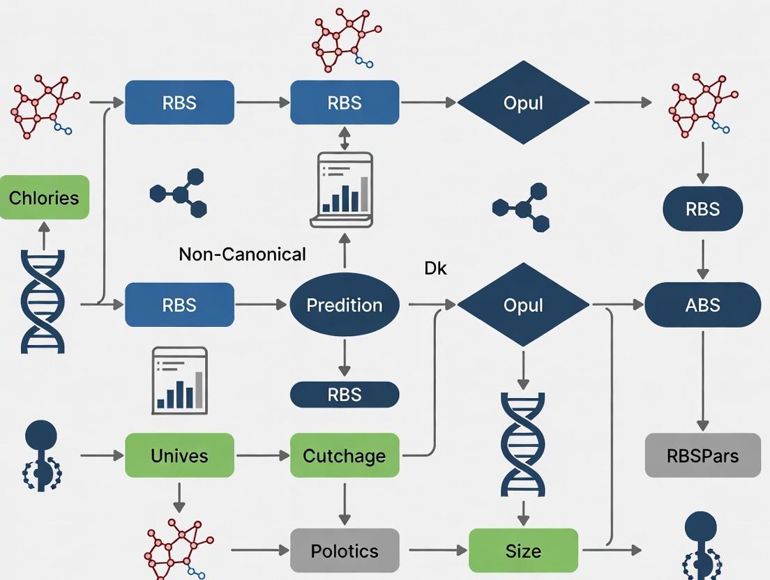
Diagram 1: Gene Prediction with Non-canonical RBS Handling
Diagram 2: Non-canonical Translation Initiation Pathways
Frequently Asked Questions (FAQs)
Q1: What are non-canonical RBS and non-canonical start codons, and how do they differ from canonical ones? A1: In canonical translation, the process begins with a defined ribosome binding site (RBS) and an AUG start codon, which is recognized by the initiator tRNA. Non-canonical mechanisms bypass these strict rules. This includes using non-canonical start codons (e.g., GTG, TTG, CTG) instead of AUG, and employing alternative RBS-independent ribosome recruitment methods like Internal Ribosome Entry Sites (IRESes) [22] [2]. These alternative start codons typically lead to a lower translation initiation efficiency, resulting in reduced protein expression levels compared to AUG [2].
Q2: What is the primary evolutionary pressure driving the use of non-canonical translation mechanisms? A2: The strongest evolutionary driver is the need to maximize coding capacity and optimize genetic information within compact genomes. RNA viruses, for instance, have very limited genome sizes (often under 30kb) and are under intense selective pressure to express multiple proteins from a single mRNA transcript. Non-canonical mechanisms enable access to overlapping open reading frames (ORFs) and allow for sophisticated gene regulation without increasing genome length [22].
Q3: During my experiment, I suspect a non-canonical ORF is functional. How can I confirm its translation is required for the observed phenotype and not just an RNA-level effect? A3: This is a critical validation step. The gold-standard experiment is start codon mutagenesis combined with a functional assay. As demonstrated in multiple studies, you should mutate the putative non-canonical start codon (e.g., from GTG to GCG) and test if the biological effect is abolished. In one case, mutating the start site in 51 ORFs resulted in a loss of the perturbational response in 48 of them (94%), confirming that the effect was mediated by translation of the ORF and not the RNA itself [13]. This should be complemented by CRISPR tiling across the locus to ensure the phenotype maps to the coding region [13] [23].
Q4: We've identified a novel microprotein from a non-canonical ORF. How can we assess its stability and potential function in cells? A4: You can employ a machine learning framework like PepScore, which was developed to calculate the probability that a non-canonical ORF-encoded peptide is stable. This model is based on ORF features such as length, presence of structured domains, and conservation [15]. For functional clues, perform ectopic expression with an epitope tag (e.g., V5) to determine the protein's subcellular localization, which can indicate potential function (e.g., nuclear, cytoplasmic, secreted) [13] [16]. Furthermore, inhibiting proteasomal and lysosomal degradation pathways can test the protein's inherent stability [15].
Q5: Are non-canonical start codons and ORFs found in prokaryotes, and do they confer an advantage? A5: Yes, they are widespread and functionally important. For example, genomic analysis of E. coli revealed that over 99% of strains use a non-canonical GTG start codon for the lacI repressor gene. This suboptimal start codon fine-tunes the basal expression level of the lactose utilization operon, providing a competitive advantage in the gut by enabling faster adaptation to available lactose [2]. This demonstrates that non-canonical start codons can serve as sophisticated metabolic tuning mechanisms.
Troubleshooting Common Experimental Challenges
| Problem | Possible Cause | Solution |
|---|---|---|
| Cannot detect microprotein via Western blot | Protein is short-lived/degraded; V5 tag may disrupt structure/function of very small proteins. | Treat cells with proteasome (e.g., MG132) and/or lysosome (e.g., chloroquine) inhibitors prior to lysis [15]. For ORFs <50 aa, consider a smaller tag or endogenous epitope tagging via CRISPR [13] [16]. |
| CRISPR knock-out shows effect, but it's unclear if it's due to the ORF or RNA | sgRNA may be disrupting a regulatory genomic element or non-coding function of the transcript. | Perform CRISPR tiling with dense sgRNAs across the entire genomic locus. A phenotype that maps exclusively to the predicted coding exon strongly suggests a protein-mediated effect [13] [23]. |
| Ribosome profiling data is noisy, confounding ORF prediction | Variable RNase digestion or lineage-specific regulation can lead to poor 3-nt periodicity. | Use computational tools like RibORF 2.0 that automate quality control, select reads with strong 3-nt periodicity, and use ribosomal A-site corrected reads for prediction. Require ORFs to be identified in multiple, independent replicates [15]. |
| Uncertain biological relevance of a predicted non-canonical ORF | The ORF may be a translational "byproduct" without function. | Conduct a focused CRISPR/Cas9 viability screen. If knock-out of the ORF impairs cell growth/survival, it indicates biological essentiality. Compare the hit rate to that of canonical genes for context (~10% for non-canonical vs. ~17% for canonical in one study) [13]. |
Key Data and Experimental Evidence
Table 1: Prevalence and Validation of Non-Canonical ORFs
The following table summarizes key quantitative findings from large-scale studies investigating non-canonical ORFs.
| Metric | Finding | Experimental Context | Source |
|---|---|---|---|
| Translated ncORFs in Human Genes | 73.5% of coding genes showed translation outside the canonical ORF (58,383 ncORFs total). | Ribosome profiling analysis of 669 human samples. | [15] |
| Functional ORFs (Viability Effect) | 57 of 553 (10%) tested non-canonical ORFs induced a viability defect upon CRISPR knock-out. | CRISPR/Cas9 loss-of-function screens in 8 cancer cell lines. | [13] |
| Protein Validation Rate | 257 of 553 (46%) produced a detectable V5-tagged protein upon ectopic expression. | Epitope-tagging and detection in human cell lines. | [13] |
| Protein vs. RNA Effect | 48 of 51 (94%) ORFs lost biological activity upon start codon mutation. | Start codon mutagenesis coupled with L1000 gene expression profiling. | [13] |
| Non-AUG Start Codon Usage | ~56.7% of human ncORFs use AUG; remainder use near-cognate codons (CTG, TTG, GTG). | Ribosome profiling and computational analysis in human, mouse, zebrafish, worm, and yeast. | [15] |
| E. coli lacI Start Codon | >99% of E. coli strains use a GTG start codon for the lacI repressor. | Genomic analysis of 10,643 E. coli genomes. | [2] |
Table 2: Essential Research Reagent Solutions
This table lists key reagents and their applications for studying non-canonical translation.
| Reagent / Tool | Function / Application | Key Consideration |
|---|---|---|
| Ribosome Profiling (Ribo-seq) | Genome-wide identification of actively translated ORFs by sequencing ribosome-protected mRNA fragments. | Data quality is paramount; ensure strong 3-nt periodicity for accurate ORF calling [15]. |
| CRISPR/Cas9 Tiling | Dense tiling of sgRNAs across a genomic locus to map the specific region essential for function. | Distinguishes between protein-coding function and regulatory DNA or functional RNA elements [13] [23]. |
| Start Codon Mutagenesis | Definitive test to confirm a phenotype is mediated by translation of an ORF and not the RNA. | Mutate the start codon to a non-functional sequence (e.g., GTG to GCG) and re-test function [13]. |
| PepScore | A logistic regression model that predicts the stability of a non-canonical ORF-encoded peptide. | Uses ORF features like expected length, encoded domain, and conservation to calculate a stability probability [15]. |
| Endogenous Epitope Tagging | Using CRISPR/Cas9 to tag an endogenous non-canonical ORF (e.g., with HA) for detection under native regulation. | Crucial for detecting low-abundance or condition-specific microproteins without overexpression artifacts [16]. |
| RibORF / RiboCode | Computational algorithms to identify translated ORFs from ribosome profiling data. | Use multiple algorithms and require consensus predictions to reduce false positives [16] [15]. |
Core Experimental Protocols
Protocol 1: Validating a Non-Canonical ORF Phenotype with Start Codon Mutagenesis
This protocol is essential for distinguishing protein-mediated effects from RNA-based mechanisms.
- Clone the Locus: Clone the genomic DNA fragment containing the putative non-canonical ORF and its endogenous regulatory context (e.g., promoter, 5' UTR) into an expression vector.
- Introduce Mutation: Using site-directed mutagenesis, mutate the predicted non-canonical start codon (e.g., GTG, TTG) to a non-functional codon (e.g., GCG, GGG). Preserve the overall RNA sequence as much as possible.
- Functional Assay: Transfect the wild-type and mutant constructs into your relevant cell line and perform the functional assay used to identify the ORF (e.g., cell viability assay, reporter gene assay, L1000 transcriptomic profiling).
- Interpretation: A significant loss of the biological activity in the start codon mutant, while the wild-type construct retains activity, strongly indicates that translation of the ORF is required for the function [13].
Protocol 2: Endogenous Tagging of a Non-Canonical ORF using CRISPR/Cas9
This protocol allows for the study of the native protein without overexpression.
- Design gRNA and Donor Template: Design a gRNA to cut near the STOP codon of the non-canonical ORF. Design a single-stranded donor DNA (ssODN) template containing the epitope tag (e.g., 3xHA) flanked by homologous arms (≥ 50 nt) matching the genomic sequence.
- Transfect and Transfert: Co-transfect cells (or generate a stable cell line) with plasmids expressing Cas9, the gRNA, and the ssODN donor template.
- Screen and Validate: Single-cell clone isolation is recommended. Screen clones by genomic PCR and sequencing to confirm precise, in-frame integration of the tag.
- Detection: Use the tagged cell line for downstream applications like Western blotting to confirm protein expression under endogenous regulation or immunoprecipitation for mass spectrometry analysis to identify interacting partners [16].
Visualization of Key Concepts
Diagram: Mechanisms of Non-Canonical Translation Initiation
From Sequence to Function: Computational and Experimental Tools for Detection
Leveraging Ribosome Profiling (Ribo-seq) to Map Actively Translated ORFs
Troubleshooting Guides: Addressing Common Ribo-seq Experimental Challenges
This section provides solutions to frequent issues encountered during Ribosome Profiling experiments, framed within the context of investigating non-canonical translation events.
Problem: Inadequate Ribosome-Protected Fragment (RPF) Yield
- Symptoms: Low library concentration, insufficient sequencing reads after rRNA depletion.
- Primary Causes & Solutions:
- Cause 1: Over-digestion by RNase. Excessive nuclease activity can degrade ribosome-protected fragments.
- Solution: Titrate RNase concentration (e.g., RNase I) and optimize digestion time and buffer conditions (e.g., 150-200 mM sodium, 5-10 mM magnesium) to achieve uniform digestion without destroying RPFs [24].
- Cause 2: Sample Loss During Library Preparation. Traditional gel-based size selection and multiple purification steps lead to significant material loss, especially with low-input samples.
- Solution: Adopt ligation-free, one-pot library preparation methods like Ribo-lite or OTTR (Ordered Two-Template Relay) that skip gel purification and reduce handling steps. These methods enable successful profiling from as few as 1,000 cells or even a single oocyte [25].
- Cause 1: Over-digestion by RNase. Excessive nuclease activity can degrade ribosome-protected fragments.
Problem: Poor Quality Data with Weak Tri-Nucleotide Periodicity
- Symptoms: Metagene analysis shows no strong 3-nucleotide (codon) periodicity at the start and stop codons; inability to confidently assign the ribosome's A and P sites.
- Primary Causes & Solutions:
- Cause 1: Ineffective Translation Arrest. Ribosome run-off during cell harvesting leads to a loss of genuine translational snapshots.
- Solution: Flash-freeze cells cryogenically or use immediate lysis with a detergent-based buffer. If using elongation inhibitors like cycloheximide, be aware of potential artifacts in ribosome distribution, particularly at the 5' end of transcripts, and validate findings with inhibitor-free protocols where possible [24].
- Cause 2: Contamination from Non-Translating RNAs. Ribosomal RNA (rRNA) can constitute over 80% of sequenced reads if not effectively removed.
- Solution: Use rigorous rRNA depletion kits (e.g., Ribo-zero Plus). Alternatively, employ computational subtraction of rRNA-derived reads post-sequencing. Newer protocols like Ribo-ITP use microfluidic isotachophoresis to physically enrich for ribosome footprints, reducing rRNA background [25].
- Cause 1: Ineffective Translation Arrest. Ribosome run-off during cell harvesting leads to a loss of genuine translational snapshots.
Problem: Data Interpretation Challenges for Non-Canonical ORFs
- Symptoms: Detecting ribosome occupancy in non-annotated regions (lncRNAs, UTRs) but lacking evidence for stable protein production.
- Primary Causes & Solutions:
- Cause 1: Distinguishing Translation from Mere Ribosome Binding. Ribosome occupancy does not always equate to productive, full-length protein synthesis [26].
- Solution: Perform CRISPR-based tiling or start codon mutagenesis. If mutating the start codon abolishes the observed phenotypic effect, it strongly indicates the effect is mediated by translation of the ORF and not the RNA itself [13].
- Cause 2: Detecting the Protein Product. Small proteins from non-canonical ORFs are often missed by standard tryptic mass spectrometry [13] [26].
- Solution: Utilize complementary methods:
- Immunopeptidomics: Identifies HLA-I presented peptides, which has proven effective for detecting peptides from non-canonical ORFs without tryptic digestion [26].
- V5/Epitope Tagging: Express the ORF with a C-terminal tag (e.g., V5) to enable detection via immunoassays. Note that tags can be disruptive for very small proteins (<50 amino acids) [13].
- Targeted Mass Spectrometry: Use methods like Selective Reaction Monitoring (SRM) to hunt for specific peptides predicted from the ORF [26].
- Solution: Utilize complementary methods:
- Cause 1: Distinguishing Translation from Mere Ribosome Binding. Ribosome occupancy does not always equate to productive, full-length protein synthesis [26].
Table 1: Critical Steps for Validating Non-Canonical ORFs
| Validation Method | Key Function | Considerations for Non-Canonical ORFs |
|---|---|---|
| CRISPR Start Codon Mutagenesis [13] | Confirms translation dependence by disrupting initiation. | Essential for distinguishing protein effects from RNA-mediated effects. |
| Ribo-seq with Periodicity [27] | Provides evidence of active, in-frame translation. | Strong 3-nt periodicity is a hallmark of productive elongation. |
| Epitope Tagging & Western Blot [13] | Confirms stable protein expression. | Tag size may interfere with function or stability of very small proteins. |
| Immunopeptidomics [26] | Detects endogenously processed and presented peptides. | Excellent for detecting stable, HLA-binding peptides; cell-type dependent. |
| Mass Spectrometry (Whole Proteome) [13] [26] | Direct detection of tryptic peptides from cellular lysates. | Low detection rate for non-canonical ORFs due to small size and low abundance. |
Problem: Difficulty in Low-Input and Single-Cell Applications
- Symptoms: Failure to generate libraries from rare cell populations or small tissue samples.
- Primary Causes & Solutions:
- Cause: Massive Sample Loss. Standard protocols require millions of cells, making small samples intractable.
- Solution: Implement specialized low-input protocols.
- Ribo-lite: A ligation-free method that skips rRNA depletion and gel purification, enabling translatome analysis from 50-1,000 cells [25].
- LiRibo-seq: Combines biotinylated-puromycin-based ribosome capture (RiboLace) with a one-pot ligation-free library prep, suitable for ~5,000 cells [25] [28].
- scRibo-seq & Ribo-ITP: True single-cell Ribo-seq methods that use either well-plate-based or microfluidic (ITP) processing to profile translation in individual cells [25].
- Solution: Implement specialized low-input protocols.
- Cause: Massive Sample Loss. Standard protocols require millions of cells, making small samples intractable.
Frequently Asked Questions (FAQs)
Q1: How does Ribo-seq fundamentally differ from RNA-seq, and why is it crucial for studying non-canonical ORFs?
RNA-seq measures the abundance and sequence of all cellular RNAs, providing a view of the transcriptome. In contrast, Ribo-seq identifies which mRNAs are actively being translated by ribosomes, providing a snapshot of the translatome. This is critical for non-canonical ORFs because many are located on transcripts annotated as non-coding (lncRNAs) or within untranslated regions (UTRs) of mRNA. RNA-seq alone would not distinguish a translated from a non-translated lncRNA, whereas Ribo-seq can reveal the active translation of a small ORF within it [24] [28].
Q2: My RNA-seq and proteomics data show poor correlation. Can Ribo-seq help explain the discrepancy?
Yes, this is a key application of Ribo-seq. The discrepancy often arises from post-transcriptional regulation, where mRNA levels do not directly predict translation rates. Ribo-seq measures the immediate step before protein synthesis (translation), effectively bridging the gap between transcript abundance and protein yield. It can reveal instances where an mRNA is abundant but poorly translated, or vice versa, providing a more direct correlate of proteome dynamics than RNA-seq [24] [28].
Q3: What is the gold-standard evidence for confirming a non-canonical ORF encodes a functional microprotein?
A multi-faceted approach is recommended:
- Translation Evidence: High-quality Ribo-seq data showing strong triplet periodicity across the putative ORF [27].
- Protein Evidence: Detection of the protein product, ideally through epitope tagging, immunopeptidomics, or targeted mass spectrometry [13] [26].
- Functional Evidence: A phenotype (e.g., viability defect, gene expression change) upon ORF knockout by CRISPR, which is abolished by start codon mutation, proving the phenotype is translation-dependent [13].
Q4: What are the best practices for visualizing Ribo-seq data to identify novel ORFs?
Use visualization tools that display reads color-coded by their reading frame, which makes the 3-nucleotide periodicity of translating ribosomes visually apparent. Tools like ggRibo (an R package) are specifically designed for this, allowing researchers to see periodicity in the context of full gene structure, including UTRs and introns, which is essential for spotting uORFs, dORFs, and ORFs in lncRNAs [27].
Q5: How can I accurately quantify global translational changes from Ribo-seq data, such as during cellular stress?
Relative analysis can be misleading during global translation shutdown. To enable absolute quantification, use spike-in controls. These can be:
- External Spike-ins: Defined synthetic RNA oligonucleotides added after RNase digestion [25].
- Orthogonal Lysates: Lysates from a different species (e.g., yeast) mixed with your sample before digestion, providing a constant reference [25].
- Internal References: Under certain conditions, mitochondrial ribosome footprints can serve as an internal control, assuming their translation is unaffected by the treatment [25].
Experimental Workflows and Visualization
The following diagrams outline the core workflows for Ribo-seq experimentation and data analysis, highlighting steps critical for investigating non-canonical ORFs.
Core Ribo-seq Wet-Lab Workflow
Computational Analysis & ORF Discovery Pipeline
The Scientist's Toolkit: Essential Research Reagents & Solutions
Table 2: Key Research Reagents and Kits for Ribo-seq Studies
| Reagent / Kit | Primary Function | Role in Studying Non-Canonical ORFs |
|---|---|---|
| Translation Inhibitors (e.g., Cycloheximide, Harringtonine) [24] | Arrests ribosomes at specific stages (elongation vs. initiation). | Harringtonine enriches for initiating ribosomes, crucial for pinpointing start codons of novel ORFs. |
| RNase I [24] | Digests unprotected mRNA, generating Ribosome-Protected Fragments (RPFs). | Produces clean RPFs for accurate mapping of translated regions, including non-canonical ones. |
| Ribo-zero Plus Kit [24] | Depletes ribosomal RNA (rRNA) from the RPF sample. | Increases the fraction of informative mRNA reads in the library, boosting signal for rare ORFs. |
| RiboLace / ALL-IN-ONE Gel Free Kit [25] [28] | Affinity-based capture of elongating ribosomes using a puromycin analog. | Gel-free workflow reduces sample loss, improves reproducibility, and is adaptable to low-input samples. |
| miRNeasy Kit [24] | Purifies small RNA fragments after nuclease digestion. | Efficiently recovers RPFs (~28-30 nt) while removing contaminants. |
Frequently Asked Questions (FAQs)
General Principles
Q: What is proteogenomics and why is it important for gene prediction research? A: Proteogenomics is the use of genomic or transcriptomic nucleotide sequencing data to create customized protein databases for mass spectrometry (MS) database searching [29]. It is crucial for gene prediction because it provides empirical evidence at the protein level to validate predicted genes, discover novel genes, and correct annotation errors, especially for non-canonical open reading frames (nORFs) that are often missed by conventional algorithms [30] [3].
Q: How does proteogenomics help in studying non-canonical RBS patterns and leaderless genes? A: Proteogenomics can experimentally validate gene expression that occurs through non-canonical patterns. Research on Deinococcus radiodurans, for example, has confirmed a −10 region-like motif (5′-TANNNT-3′) functioning as a promoter immediately upstream of ORFs, producing leaderless mRNA without a Shine–Dalgarno (SD) sequence [31]. This allows proteogenomics to detect and provide evidence for proteins expressed from such non-canonical genes.
Technical Challenges
Q: Why are noncanonical proteins often missed in standard proteomic analyses? A: Noncanonical proteins, often encoded by small open reading frames (sORFs), present unique challenges: their often small size, low abundance, non-AUG initiation, and rapid turnover make them difficult to detect using conventional proteomic approaches [3]. Standard gene prediction algorithms also typically prioritize ORFs exceeding 100 codons, systematically overlooking sORFs with validated coding potential [30].
Q: What are common reasons for the failure to detect peptides in a proteogenomic experiment? A: Failure can occur due to sample loss during processing, protein degradation, or unsuitable peptide sizes post-digestion [32]. Low-abundant proteins can be lost during preparation or be undetectable next to high-abundance proteins. Peptides may also "escape detection" if they are too long or too short due to suboptimal digestion [32].
Q: How can I improve the detection of low-abundance or non-canonical proteins? A: Scale up the experiment, increase relative protein concentration using cell fractionation, or enrich low-abundance proteins by Immunoprecipitation (IP) [32]. Using a combination of two different proteases (double digestion) can also help generate a more suitable range of peptide sizes for detection [32].
Troubleshooting Guides
Problem: High False Discovery Rate or Poor Spectral Matching
| Potential Cause | Diagnostic Check | Solution |
|---|---|---|
| Incomplete or generic protein database | Check if your custom database includes sample-specific variants and novel ORFs. | Create a comprehensive custom database using RNA-Seq data from the same sample to include novel splice junctions, SAVs, and indels [33] [29]. |
| Suboptimal mass spectrometer calibration | Check instrument performance with a standard HeLa protein digest [34]. | Clean and recalibrate the mass spectrometer using a commercial calibration solution [34]. |
| Incorrect search parameters | Verify search settings in your software (e.g., Mascot Score, P-value). | Ensure parameters like species, enzyme, fragment ions, and mass tolerance are correctly set. Use a P-value/Q-value of < 0.05 or a significant Mascot Score for validation [32]. |
Problem: Low Protein Coverage or Peptide Count
| Potential Cause | Diagnostic Check | Solution |
|---|---|---|
| Protein degradation during processing | Monitor each preparation step by Western Blot or Coomassie staining [32]. | Add broad-spectrum, EDTA-free protease inhibitor cocktails to all buffers during sample prep [32]. |
| Inefficient enzymatic digestion | Evaluate peptide size range and coverage. | Optimize digestion time or change the protease type (e.g., trypsin vs. Lys-C). Consider double digestion with two different proteases [32]. |
| High sample complexity masking low-abundance targets | Assess the number of proteins and dynamic range in your sample. | Fractionate complex samples using a high-pH reversed-phase peptide fractionation kit to reduce complexity [34]. |
Problem: Inability to Validate Predicted Novel Genes
| Potential Cause | Diagnostic Check | Solution |
|---|---|---|
| Limitations of gene prediction algorithms | Check if initial gene models were based only on ab initio prediction. | Perform a multi-stage proteogenomic analysis across different biological conditions (e.g., life cycle states) to capture condition-specific expression [30]. |
| Low expression of non-canonical ORFs | Check RNA-Seq data (e.g., FPKM) for the locus of interest. | Use ribosome profiling (Ribo-seq) to provide evidence of translation, then target the specific peptide with PRM or MRM MS assays [3] [35]. |
Key Experimental Protocols
Protocol 1: Creating a Custom Protein Database from RNA-Seq Data
This protocol is essential for detecting sample-specific variations and non-canonical proteins [33] [29].
- Data Upload and Preparation: Import the reference genome (FASTA), RNA-seq reads (FASTQ), and gene annotation file (GTF). Ensure chromosome naming conventions are consistent (e.g., change "1" to "chr1") using a text replacement tool [33].
- Read Alignment: Use a splice-aware aligner like HISAT2 to map the RNA-Seq reads (FASTQ) to the reference genome. This generates a BAM file containing the alignment information [33].
- Variant Calling: Use a variant caller like FreeBayes on the BAM file to identify single-nucleotide polymorphisms (SNPs) and insertions/deletions (indels). This outputs a VCF file [33].
- Database Generation: Translate the identified variants and de novo assembled transcripts into amino acid sequences. Merge these with the reference protein database (e.g., from UniProt) to create a comprehensive, sample-specific FASTA database [33] [36].
Protocol 2: Multi-State Proteogenomic Analysis for Gene Discovery
This protocol, adapted from a Tetrahymena thermophila study, is designed to comprehensively reassess gene discovery across different biological conditions [30].
- Experimental Design:
- Select multiple distinct biological or environmental states relevant to your organism (e.g., growth, starvation, conjugation).
- Harvest cells from each state independently.
- Sample Preparation and Fractionation:
- Prepare total protein extracts from each state.
- To increase depth, process aliquots of the lysate using both in-gel and in-solution tryptic digestion.
- Pre-fractionate the in-solution digested peptides using reversed-phase HPLC (e.g., on a TechMate C18 column) to reduce complexity.
- Mass Spectrometry Data Acquisition:
- Analyze all peptide fractions on a high-resolution mass spectrometer (e.g., Q Exactive HFX).
- Consolidate proteomic data for each state by integrating results from both digestion protocols.
- Database Search and Novel Event Identification:
- Search the consolidated MS data against your custom protein database using search engine software (e.g., pFind in open search mode).
- Use integrated software (e.g., GAPE) to identify peptides, novel genes, and post-translational modifications.
- Bioinformatic Validation:
- Functionally annotate identified proteins using KOG and GO terms.
- Determine the correlation between transcriptomic (FPKM) and proteomic (NSAF) expression levels.
- Perform cluster analysis to identify proteins and PTMs associated with specific states.
Experimental Workflow and Data Integration
The following diagram illustrates the core proteogenomic workflow for validating gene models, integrating genomics, transcriptomics, and proteomics data.
Research Reagent Solutions
The following table details key reagents and kits used in proteogenomic workflows for reliable results.
| Item | Function | Example Use Case |
|---|---|---|
| Pierce HeLa Protein Digest Standard [34] | Verifies overall MS instrument performance and sample preparation protocol. | Run as a control to determine if poor results are from sample prep or the LC-MS system. |
| Pierce Peptide Retention Time Calibration Mixture [34] | Diagnoses and troubleshoots the Liquid Chromatography (LC) system and gradient. | Ensures consistent peptide elution times, critical for reproducible LC-MS/MS runs. |
| Pierce Calibration Solutions [34] | Calibrates the mass spectrometer for accurate mass measurement. | Regular instrument calibration to maintain mass accuracy, essential for peptide identification. |
| Protease Inhibitor Cocktails (EDTA-free) [32] | Prevents protein degradation during sample preparation. | Added to lysis and extraction buffers to preserve protein integrity, especially for low-abundance targets. |
| High pH Reversed-Phase Peptide Fractionation Kit [34] | Reduces sample complexity by fractionating peptides before MS analysis. | Used with complex samples (e.g., TMT-labeled) to improve depth of coverage and detect low-abundance proteins. |
| Trypsin (or alternative proteases) [32] | Digests proteins into peptides suitable for MS analysis. | Standard enzyme for proteolysis. Changing protease type or using double digestion can improve coverage of problematic proteins. |
Frequently Asked Questions (FAQs)
Q1: Why do standard gene prediction tools often fail to correctly identify short ORFs? Standard gene prediction tools frequently miss or mis-annotate short open reading frames (sORFs, <100 codons) for several key reasons. Firstly, many gene annotation pipelines deliberately ignore sORFs, often setting an arbitrary cutoff (e.g., 100 codons) and dismissing anything shorter as non-functional [37] [38]. Secondly, the statistical models (e.g., codon usage indices) and homology search methods (like BLAST) used by conventional tools are optimized for longer, typical genes and perform poorly on sORFs due to their limited sequence length [37]. This is compounded by the fact that databases contain very few experimentally verified sORFs for training and comparison, making homology-based detection unreliable [37]. Consequently, a significant number of genuine sORFs are incorrectly annotated as 'hypothetical' or 'putative' proteins [38].
Q2: What are non-canonical RBS patterns, and why are they problematic for prediction? Non-canonical Ribosome Binding Site (RBS) patterns are translation initiation signals that deviate from the standard Shine-Dalgarno (SD) sequence (5'-AGGAGG-3').
- Leaderless mRNAs: These transcripts completely lack a 5' untranslated region (5'-UTR), meaning translation starts directly at the 5' end. This mode is abundant in archaea and certain bacterial groups [12] [1].
- Non-SD RBSs: Many mRNAs possess alternative, often weaker, sequence patterns in their 5' UTR that are not complementary to the anti-Shine-Dalgarno sequence [39] [1]. It is estimated that approximately half of bacterial genes may lack a canonical SD sequence [1].
- Other Initiation Mechanisms: Recent research has identified additional non-canonical mechanisms, such as initiation mediated by a 5'-terminal AUG codon (5'-uAUG) that attracts 70S ribosomes, compensating for a poor downstream SD sequence [1].
These patterns are problematic because most ab initio gene finders are primarily trained to recognize canonical SD sequences, leading to inaccurate prediction of translation start sites for genes with atypical RBSs [12].
Q3: How do advanced tools like StartLink+ and MetaGeneAnnotator improve gene start prediction? Next-generation predictors use innovative strategies to overcome the limitations of standard tools.
- StartLink+ combines ab initio prediction with a homology-based approach. It uses multiple sequence alignments of homologous nucleotide sequences to identify conserved start codon patterns. When its prediction matches that of an ab initio algorithm (GeneMarkS-2), the accuracy is exceptionally high (98-99%) [12].
- MetaGeneAnnotator (MGA) integrates specialized statistical models for prophage genes alongside bacterial and archaeal models. A key feature is its self-training model that adapts to the di-codon usage of the input sequence itself, making it sensitive to atypical genes. It also employs a sophisticated, species-specific RBS model that can detect non-canonical patterns, leading to more precise translation start site identification [20].
Q4: What experimental validation methods are available for predicted short ORFs and gene starts? Computational predictions should be confirmed experimentally. The primary methods for validating gene starts include:
- N-terminal protein sequencing: This is a classical method for directly determining the start of a protein. Studies in E. coli and Mycobacterium tuberculosis have used this to create benchmark datasets [12].
- Mass spectrometry: This technique is powerful for identifying proteins and, with specific protocols, can be used to characterize their N-termini [12].
- Ribosome profiling (Ribo-Seq): This method maps the positions of all ribosomes on an mRNA, providing direct evidence of translation initiation events, including those from non-canonical sites [22].
- Mutagenesis: Introducing frameshift mutations or mutating the start codon can be used to test if a predicted ORF is functional [12].
Comparative Accuracy of Gene Start Prediction Tools
Table 1: Performance of different gene prediction methodologies on prokaryotic genomes.
| Tool / Method | Primary Approach | Key Strength | Reported Accuracy on Experimentally Verified Starts |
|---|---|---|---|
| StartLink+ | Hybrid (Alignment + Ab initio) | Resolves ambiguous starts by requiring consensus. | 98 - 99% [12] |
| StartLink | Alignment-based | Infers starts from conserved homologs; works on short contigs. | High, but limited to genes with sufficient homologs [12] |
| GeneMarkS-2 | Ab initio | Uses multiple models for SD, non-SD, and leaderless initiation. | High, but starts often disagree with other tools [12] |
| MetaGeneAnnotator | Ab initio | Self-training model and species-specific RBS detection. | Precisely predicts translation starts on anonymous sequences [20] |
| Prodigal | Ab initio | Optimized for canonical Shine-Dalgarno (SD) RBSs. | Performance drops with non-canonical RBS patterns [12] |
Performance of sORF Prediction Methods inS. cerevisiae
Table 2: A comparison of computational methods for predicting small Open Reading Frames (sORFs) based on a study in Saccharomyces cerevisiae [37].
| Method | Type | True Positive Rate at 5% False Positive Rate (1-99 codons) | Overall Assessment |
|---|---|---|---|
| BLAST (Homology Search) | Similarity-based | Low performance due to limited verified sORFs in databases. | Poor for novel sORFs, depends on existing knowledge [37] |
| sORF finder | Ab initio | Similar accuracy to homology search for sORFs. | Designed specifically for sORFs; uses hexamer composition bias [37] |
| CodonW (Codon Usage) | Ab initio | Performs poorly for small genes. | Effective for standard genes but unreliable for sORFs [37] |
Troubleshooting Guides
Problem: Inconsistent Gene Start Predictions Between Tools
Potential Cause: The gene in question likely uses a non-canonical translation initiation mechanism (e.g., leaderless transcription, a non-SD RBS, or an unknown mechanism) that is modeled differently by each tool [12] [1].
Solution:
- Run a specialist tool: Use a predictor designed for non-canonical patterns, such as GeneMarkS-2 or MetaGeneAnnotator, which model multiple types of RBSs and leaderless initiation [20] [12].
- Employ a hybrid approach: Use StartLink+ if possible. Its consensus-based approach is highly reliable where it produces a result [12].
- Conduct a manual check:
- Examine the upstream region of the predicted gene for obvious canonical SD sequences.
- Look for known non-canonical signals, such as A/U-rich regions that might bind ribosomal protein S1 [1] or a 5'-uAUG [1].
- Check for phylogenetic conservation of the upstream region across homologs, which can indicate a functional but non-canonical RBS.
This workflow for resolving conflicting gene start predictions integrates multiple tools and validation strategies:
Problem: Failure to Detect Potential Short ORFs in Genomic Data
Potential Cause: The standard gene-finding pipeline is configured with a minimum ORF length cutoff that excludes sORFs, or the statistical model is not sensitive enough to distinguish real sORFs from random noise [37] [38].
Solution:
- Use sORF-specific prediction software: Employ tools explicitly designed for sORF discovery, such as sORF finder, which uses hexamer composition bias between coding and non-coding sequences [37].
- Adjust pipeline parameters: If using a standard gene finder, lower the minimum ORF length threshold, but be aware this will generate many false positives that require further filtering [37].
- Integrate multi-omics evidence: Incorporate data from ribosome profiling (Ribo-Seq) or mass spectrometry to provide experimental evidence of translation, which can help validate computational predictions [22] [12].
Research Reagent Solutions: Essential Tools for Gene Prediction Research
Table 3: Key computational tools and resources for advanced gene prediction work.
| Tool / Resource | Function | Application Context |
|---|---|---|
| StartLink+ | Hybrid gene start predictor | High-accuracy annotation of gene starts in prokaryotes; resolving tool conflicts [12]. |
| GeneMarkS-2 | Self-training ab initio gene finder | Predicting genes in standard and novel genomes, especially with mixed initiation mechanisms [12]. |
| MetaGeneAnnotator (MGA) | Ab initio gene finder | Gene prediction on short, anonymous sequences (e.g., metagenomes); precise RBS detection [20]. |
| sORF finder | sORF discovery tool | Identifying small ORFs with high coding potential [37]. |
| Recode Database | Database of recoding events | Curated resource for genes using programmed frameshifting or stop-codon readthrough [40]. |
| AUGUSTUS | Eukaryotic gene predictor | Predicting genes in eukaryotic genomic sequences [21]. |
Accurate gene prediction is a cornerstone of genomics, yet the identification of precise gene starts remains a significant challenge, especially for genes with non-canonical Ribosome Binding Site (RBS) patterns. Traditional computational tools often disagree on start codon predictions for a substantial portion of genes in a genome, with discrepancies ranging from 15% to 25% [12]. This problem is exacerbated in genomes with a high GC content and for genes that utilize non-canonical initiation mechanisms, such as leaderless transcription or non-Shine-Dalgarno RBSs [12]. These non-canonical patterns elude models trained predominantly on standard sequences, leading to incomplete or inaccurate genome annotations. This technical support article explores how deep learning architectures, specifically Convolutional Neural Networks (CNNs) and Transformers, can be leveraged to address these challenges, providing researchers with advanced methodologies for improved sequence analysis.
Deep Learning Architectures for Sequence Analysis
Convolutional Neural Networks (CNNs)
CNNs are deep learning algorithms particularly effective for identifying local, spatially-invariant patterns in data.
- Core Mechanism: Their architecture is built around convolutional layers that apply filters to scan input sequences, detecting local features regardless of their position. This is followed by pooling layers that reduce dimensionality and a fully connected layer for final output mapping [41].
- Application to Sequence Analysis: In genomic sequences, CNNs excel at identifying short, conserved motifs—such as promoter elements, splice sites, or short RBS patterns—by scanning the nucleotide sequence with these convolutional filters [41]. Their strength lies in capturing local dependencies within a defined window.
Transformer Models
Transformers are a neural network architecture based on a self-attention mechanism, allowing them to model long-range dependencies and contextual relationships across an entire sequence.
- Core Mechanism: Self-Attention: The self-attention mechanism computes query, key, and value vectors for each element (e.g., nucleotide or token) in the input sequence. It then calculates alignment scores to determine how much each element should "attend to" every other element when encoding information [42]. This allows the model to weigh the importance of different parts of the sequence globally, rather than just locally.
- Application to Sequence Analysis: For genomic sequences, Transformers can capture the context of a potential start codon by analyzing the entire upstream region and even parts of the coding sequence simultaneously. This is crucial for interpreting non-canonical RBS patterns whose signals may be diffuse or context-dependent [43] [42].
Comparative Analysis: CNNs vs. Transformers
The table below summarizes the key characteristics of CNNs and Transformers in the context of genomic sequence analysis.
Table 1: Comparison of CNN and Transformer Architectures for Sequence Analysis
| Feature | Convolutional Neural Networks (CNNs) | Transformer Models |
|---|---|---|
| Core Strength | Excellent at identifying local, position-invariant patterns and motifs [41]. | Excels at capturing long-range dependencies and global context across a sequence [42]. |
| Handling Long-Range Context | Limited; restricted by the size of the convolutional kernel and network depth. Struggles with correlations between distant elements [41] [42]. | Superior; self-attention theoretically connects every position in the sequence to every other position in a single layer. |
| Computational Resources | Generally more efficient and less computationally demanding, suitable for large-scale screening [41]. | computationally expensive due to the self-attention mechanism, which requires resources quadratic to the sequence length [43]. |
| Interpretability | Often easier to interpret which local features (motifs) contributed to a prediction. | Can be interpreted via attention weights to see which parts of the sequence the model found important, though this can be complex. |
Technical Support Center: FAQs & Troubleshooting Guides
Frequently Asked Questions (FAQs)
Q1: My model for predicting translation initiation sites (TIS) performs well on canonical AUG codons but poorly on non-AUG start codons. What can I do?
- A: This is a common issue. First, ensure your training dataset is balanced and includes confirmed examples of non-AUG initiation (e.g., CUG, GUG, UUG). Consider using ribosome profiling (Ribo-seq) data from studies that specifically investigated non-canonical translation to curate positive examples [11]. Secondly, a Transformer model may be more suitable than a CNN here, as non-AUG initiation often relies on broader sequence context and structural features that self-attention mechanisms are adept at capturing.
Q2: How can I determine if my gene prediction model is effectively learning the biology of translation initiation and not just sequence artifacts?
- A: Employ rigorous validation strategies. Perform in silico saturation mutagenesis on the upstream untranslated region (UTR) of known genes and see if the model's predictions change in a biologically plausible way (e.g., disrupting a conserved Shine-Dalgarno sequence drops the prediction score). Furthermore, correlate your model's high-confidence predictions for non-canonical ORFs with experimental evidence, such as mass spectrometry data or results from CRISPR-based functional screens, which can confirm the expression and biological activity of the predicted proteins [13] [5].
Q3: What is the significance of "leaderless transcription" and how can my model account for it?
- A: Leaderless transcription occurs when a gene starts directly with the start codon, lacking a 5' UTR and thus a canonical RBS. In some archaea and bacteria, this can be the predominant mode of transcription [12]. Models trained only on genes with leadered transcripts will fail for these cases. To account for this, incorporate promoter signal patterns as additional input features, as the transcription start site is adjacent to the translation start site. Using a Transformer model can also be beneficial, as it can directly learn the relationship between the promoter and the start codon without being constrained by a fixed-length RBS search window.
Troubleshooting Guide
Table 2: Troubleshooting Common Issues in Deep Learning-Based Gene Start Prediction
| Problem | Potential Causes | Solutions |
|---|---|---|
| High false positive rate for gene starts in AT-rich intergenic regions. | Model is mistaking random ATG codons in non-coding regions for genuine start sites. | 1. Incorporate conservation data; true sites are often more evolutionarily conserved. Tools like StartLink use this principle [12]. 2. Add chromatin accessibility or histone modification data as additional input to distinguish active regulatory regions. |
| Model performs well on training data but generalizes poorly to new, unrelated genomes. | Overfitting to taxon-specific sequence biases in the training set. | 1. Increase the diversity of species in your training data. 2. Apply data augmentation techniques, such as reverse-complementing sequences or adding mild random noise. 3. Use transfer learning: pre-train on a large, diverse dataset, then fine-tune on your specific organism of interest. |
| Computational runtimes are prohibitively long, slowing down research iteration. | Model architecture may be too complex for the task (e.g., using a large Transformer for a simple motif-finding task). | 1. For tasks focused on local motif discovery, try a simpler CNN architecture first [41]. 2. If using a Transformer, consider using a more efficient variant or reducing the sequence context window. 3. Ensure you are leveraging GPU acceleration and have optimized your data input pipeline. |
Experimental Protocol: Integrating Ribo-seq and Mass Spectrometry for Functional Validation
A critical step in studying non-canonical translation is to experimentally validate the predicted products. The following integrated protocol outlines this process.
Ribosome Profiling (Ribo-seq):
- Purpose: To map the exact positions of translating ribosomes across the transcriptome at nucleotide resolution. This identifies actively translated ORFs, including non-canonical ones like upstream ORFs (uORFs) and ORFs in long non-coding RNAs (lncRNAs) [11].
- Methodology: Treat cells with a drug like cycloheximide to arrest translating ribosomes. Nuclease-footprint the protected mRNA fragments (~30 nucleotides) bound by ribosomes. Construct a sequencing library from these footprints and sequence them. The resulting data reveals the three-nucleotide periodicity of ribosome-protected fragments, pinpointing translated regions [13] [11].
Mass Spectrometry (MS) Proteomics:
- Purpose: To obtain direct evidence of protein synthesis from predicted non-canonical ORFs.
- Methodology:
- Sample Preparation: Lyse cells and digest proteins into peptides.
- Liquid Chromatography-Tandem Mass Spectrometry (LC-MS/MS): Separate peptides by liquid chromatography and analyze them with tandem MS. Fragment the peptides and measure the mass-to-charge ratio of the resulting ions.
- Database Search: Search the acquired spectra against a custom database that includes the predicted non-canonical ORFs from your Ribo-seq analysis and in silico predictions. The identification of unique, high-confidence peptide spectra matches (PSMs) confirms the expression of the novel protein [13] [5].
Functional Validation via CRISPR Screening:
- Purpose: To assess the biological relevance of the validated non-canonical proteins.
- Methodology: Design a CRISPR/Cas9 guide RNA (sgRNA) library targeting the confirmed non-canonical ORFs. Transduce a population of cells (e.g., a cancer cell line) with this library and perform a negative selection screen. ORFs whose knockout impairs cell viability or growth indicate essential biological functions, underscoring their importance [13] [11].
The logical flow of this integrated experimental approach is summarized in the diagram below.
Integrated Experimental Workflow for Non-Canonical Gene Validation
The Scientist's Toolkit: Key Research Reagents & Solutions
Table 3: Essential Reagents and Tools for Investigating Non-Canonical Translation
| Research Reagent / Tool | Function / Application | Example Use in Experiments |
|---|---|---|
| Cycloheximide | A translation inhibitor that arrests ribosomes, stabilizing them on mRNA for Ribo-seq. | Used in Ribo-seq protocol to capture ribosome-protected mRNA fragments, allowing for the mapping of translated ORFs [13]. |
| CRISPR/Cas9 sgRNA Library | A pooled library of guide RNAs designed to knock out specific target genes. | Used in functional screens to determine if the knockout of a predicted non-canonical ORF affects cell viability or proliferation, indicating biological importance [13] [11]. |
| V5 Epitope Tag | A short peptide tag that can be fused to a protein of interest for detection. | Fused to candidate non-canonical ORFs for ectopic expression; anti-V5 antibodies are then used in western blot or immunofluorescence to confirm protein expression and subcellular localization [13]. |
| StartLink+ Algorithm | A computational tool that combines ab initio and homology-based methods to accurately predict gene starts. | Used to improve the annotation of gene starts in prokaryotic genomes, especially those with non-canonical RBS patterns or leaderless transcription, providing a benchmark for model training [12]. |
| Custom Peptide Database | A curated database of theoretical peptide sequences derived from predicted non-canonical ORFs. | Essential for MS proteomics; used to search and identify mass spectra that confirm the existence of novel peptides, moving beyond predictions to direct physical evidence [11] [5]. |
Troubleshooting Guides and FAQs
Frequently Asked Questions
Q1: What are the main types of non-canonical RBS patterns, and how do they impact gene prediction?
Non-canonical RBS patterns deviate from the typical Shine-Dalgarno consensus and can include motifs associated with leaderless transcription, where genes start immediately without a 5' untranslated region (5' UTR) or a canonical RBS [44]. Some species exhibit RBS sites that do not follow the Shine-Dalgarno consensus at all, even for leadered genes [44]. These variations impact gene prediction by causing algorithms to miss true gene starts or entire genes if they rely solely on canonical models.
Q2: My gene prediction tool is missing known nORFs in my prokaryotic data. What steps can I take?
First, verify that you are using a tool specifically designed to handle atypical genetic elements. Tools like MetaGeneAnnotator (MGA) and GeneMarkS-2 incorporate models for prophage genes, horizontally transferred genes, and non-canonical RBS patterns, which significantly improve sensitivity to nORFs [20] [44]. Ensure your tool uses a self-training model from the input sequences to adapt to species-specific signals [20]. You can also run a comparative analysis using multiple dedicated algorithms and cross-reference the results.
Q3: How can I experimentally validate predicted nORFs and their translation products?
Ribosome profiling is a key method for observing the translation of non-canonical ORFs [45]. Furthermore, functional validation can be achieved through CRISPR-Cas9 screens to identify nORFs essential for cell survival, as demonstrated in medulloblastoma research [45]. For investigating the regulatory elements controlling nORF expression, newer high-throughput methods like Variant-EFFECTS can quantify how specific DNA edits affect gene expression in an endogenous context [46].
Q4: What are common pitfalls in interpreting ribosome profiling data for nORFs?
A major pitfall is the assumption that ribosome-protected fragments unequivocally indicate functional protein synthesis. It is crucial to integrate data from multiple sources, such as proteomics experiments [44] and mass spectrometry data, to confirm the production of stable proteins. Additionally, technical artifacts from sample preparation or data analysis can lead to false positives, emphasizing the need for robust bioinformatics controls.
Q5: How can I troubleshoot low yield or quality in sequencing preparation for nORF studies?
Refer to the following table for common issues and solutions in Next-Generation Sequencing (NGS) library preparation [47].
Table: Troubleshooting Common NGS Library Preparation Issues
| Problem Category | Typical Failure Signals | Common Root Causes | Corrective Actions |
|---|---|---|---|
| Sample Input / Quality | Low starting yield; smear in electropherogram; low library complexity | Degraded DNA/RNA; sample contaminants (phenol, salts); inaccurate quantification | Re-purify input sample; use fluorometric quantification (e.g., Qubit) instead of UV absorbance only. |
| Fragmentation & Ligation | Unexpected fragment size; inefficient ligation; adapter-dimer peaks | Over- or under-shearing; improper buffer conditions; suboptimal adapter-to-insert ratio | Optimize fragmentation parameters; titrate adapter:insert molar ratios; ensure fresh ligase. |
| Amplification & PCR | Overamplification artifacts; bias; high duplicate rate | Too many PCR cycles; inefficient polymerase or inhibitors | Reduce the number of PCR cycles; use high-fidelity polymerases; ensure clean input sample. |
| Purification & Cleanup | Incomplete removal of small fragments; sample loss; carryover of salts | Wrong bead ratio; bead over-drying; inefficient washing | Precisely follow bead cleanup protocols; avoid over-drying beads; use fresh wash buffers. |
The Scientist's Toolkit: Key Research Reagent Solutions
Table: Essential Reagents and Kits for nORF and Regulatory Element Research
| Item | Function | Example Use Case |
|---|---|---|
| CRISPR Prime Editing System (PE2) | Precisely introduces designed sequence edits into the genome without double-strand breaks [46]. | Creating specific mutations in regulatory DNA to study their effect on nORF expression in Variant-EFFECTS [46]. |
| Ribosome Profiling Kits | Provide reagents for capturing and sequencing ribosome-protected mRNA fragments. | Genome-wide identification of translated nORFs, even those that are non-canonical [45]. |
| Flow-FISH Assay Kits | Enable detection and quantification of specific RNA transcripts in single cells using flow cytometry. | Measuring the effects of regulatory DNA edits on target gene expression in Variant-EFFECTS screens [46]. |
| Validated NGS Library Prep Kits | Ensure high-efficiency, low-bias library construction for sequencing. | Generating high-quality RNA-Seq and ribosome profiling libraries for accurate nORF detection [47]. |
Experimental Protocols for nORF Research
Protocol 1: Identifying Functional nORFs via CRISPR-Cas9 Screens
This protocol is adapted from a study on childhood medulloblastoma [45].
- Design and Library Cloning: Design a library of single-guide RNAs (sgRNAs) targeting predicted nORFs genome-wide, along with non-targeting control sgRNAs.
- Virus Production: Package the sgRNA library into a lentiviral vector to produce virus at a low multiplicity of infection (MOI) to ensure one integration per cell.
- Cell Transduction and Selection: Transduce the target cells (e.g., medulloblastoma cell lines) with the lentiviral library and select with antibiotics.
- Screening and Passaging: Passage the cells for several weeks, harvesting a portion of the population at each passage to track sgRNA abundance over time.
- Sequencing and Analysis: Extract genomic DNA from all time points and amplify the integrated sgRNA sequences for high-throughput sequencing. sgRNAs that drop out over time indicate that the targeted nORF is essential for cell survival.
Protocol 2: Dissecting Regulatory Elements with Variant-EFFECTS
This protocol describes how to measure the effect of regulatory DNA edits on gene expression [46].
- Edit and pegRNA Design: Design a library of hundreds of specific sequence edits (e.g., tiling mutations, TF motif insertions) for a regulatory element of interest. Encode these edits into a library of prime editing guide RNAs (pegRNAs).
- Cell Line Preparation: Establish a cell line (e.g., THP-1, Jurkat) with stable, inducible expression of the Prime Editor 2 (PE2) system.
- Library Transduction and Editing: Transduce the pegRNA library via lentivirus into the PE2-expressing cells. Induce PE2 expression with doxycycline for a prolonged period (e.g., 14+ days), then remove doxycycline to allow PE2 degradation.
- Cell Sorting by Expression: Label cells based on the expression level of the target gene using RNA FlowFISH or a fluorescent antibody. Use Fluorescence-Activated Cell Sorting (FACS) to sort cells into multiple bins based on expression level.
- Genotype Analysis and Effect Quantification: Extract genomic DNA from each sorted bin, PCR-amplify the edited genomic region, and sequence it. Use a computational analysis pipeline to estimate the quantitative effect of each designed edit on gene expression, accounting for editing efficiency and cell ploidy.
Workflow and Signaling Pathway Visualizations
Diagram: High-Level Workflow for Building a nORF Catalog
Diagram: Variant-EFFECTS Experimental Workflow
Navigating Predictive Challenges: Pitfalls and Optimization Strategies
Addressing High False-Positive Rates and Improving Specificity in Predictions
Frequently Asked Questions (FAQs)
Q1: Why do my gene predictions have high false-positive rates when working with non-canonical RBS patterns? High false-positive rates often occur because standard prediction tools are trained primarily on canonical genetic sequences and patterns. When encountering non-canonical ribosome binding site (RBS) patterns, these tools may misinterpret regulatory signals, leading to incorrect positive identifications. The algorithms' scoring matrices and threshold parameters are typically optimized for standard sequences, causing reduced specificity with atypical genetic architectures [48].
Q2: What computational approaches can improve prediction specificity for non-canonical sequences? Implementing multi-tool consensus strategies and leveraging recently benchmarked algorithms significantly enhances specificity. According to 2025 benchmarking research, Numbat and CopyKAT have demonstrated superior performance in distinguishing true signals from background noise in complex genomic data. Combining these tools with experimental validation creates a robust framework for reducing false positives [49].
Q3: How does experimental design affect false-positive rates in genetic prediction studies? Proper experimental design critically impacts false-discovery rates. Research indicates that implementing Design of Experiments (DoE) methodology with structured multivariate approaches allows for more efficient exploration of complex genetic design spaces while controlling for confounding variables. This systematic approach enables researchers to identify true positive signals amidst noisy data, particularly when working with non-canonical genetic elements like atypical RBS patterns [50].
Q4: What validation methods are most effective for confirming predictions involving non-canonical RBS? A tiered validation approach provides the most reliable confirmation:
- Primary validation through Sanger sequencing for high accuracy on limited targets
- Secondary confirmation via high-throughput sequencing (NGS) for broader coverage
- Functional validation through expression assays measuring protein output This multi-layered approach ensures predictions are accurate across sequence, structural, and functional dimensions [51].
Troubleshooting Guides
Problem: Consistently High False-Positive Rates in RBS Prediction
Symptoms:
- Predictions fail validation sequencing
- Multiple overlapping false-positive hits in intergenic regions
- Inconsistent results across different prediction tools
Solution Steps:
Tool Selection and Benchmarking
- Utilize recently benchmarked algorithms shown to perform well with non-canonical sequences
- Implement Numbat for comprehensive analysis when computational resources allow
- Use CopyKAT as a reliable alternative for large-scale screening studies [49]
Parameter Optimization
- Adjust scoring thresholds based on empirical validation data
- Implement length constraints to filter biologically implausible predictions
- Incorporate species-specific genetic content parameters when available
Multi-Tool Consensus Approach
- Run predictions through at least two independently developed algorithms
- Consider only predictions identified by multiple tools as high-confidence hits
- Use the following table to select complementary tool pairs:
Table: Benchmark Performance of Prediction Tools for Non-Canonical Sequences
| Tool Name | Best Application Context | Reported Specificity | Key Strengths | Computational Demand |
|---|---|---|---|---|
| Numbat | Comprehensive analysis | Highest in benchmark [49] | Optimal balanced performance | High |
| CopyKAT | Large-scale screening | High (recommended alternative) [49] | Good speed/accuracy balance | Medium |
| Traditional BLAST | Canonical sequences only | Low with non-canonical patterns [48] | Fast, widely available | Low |
- Experimental Validation Design
- Implement orthogonal validation methods (sequencing + functional assays)
- Include appropriate positive and negative controls in each experiment
- Utilize DoE principles to optimize validation efficiency [50]
Problem: Inconsistent Prediction Results Across Platforms
Symptoms:
- Different results from the same input data on different computational platforms
- Reproducibility challenges between research groups
- Version-dependent variation in prediction outcomes
Solution Steps:
Computational Environment Standardization
- Document and control software versions, including dependencies
- Implement containerization (Docker/Singularity) for reproducible environments
- Standardize reference databases and version control
Input Data Quality Control
- Verify sequence quality metrics before analysis
- Implement adapter and quality trimming appropriate to your sequencing platform
- Establish minimum coverage thresholds for reliable calling
Benchmarking with Reference Datasets
- Maintain a set of validated positive and negative control sequences
- Run controls with each analysis batch to monitor performance drift
- Compare against community-standard reference sets when available
Experimental Protocols
Protocol 1: Orthogonal Validation of Predicted Non-Canonical RBS Elements
Purpose: Confirm computational predictions of non-canonical RBS patterns using multiple experimental methods to minimize false positives.
Materials:
- DNA template containing predicted RBS
- Validation primers flanking predicted region
- Sanger sequencing reagents or NGS library preparation kit
- Cell-free expression system for functional validation
- Antibodies or reporter systems for detection
Procedure:
Amplification and Cloning
- PCR amplify region containing predicted RBS using high-fidelity polymerase
- Clone into validation vector with appropriate selection markers
- Transform into competent cells and pick multiple colonies for sequencing
Sequential Validation
- Perform Sanger sequencing of cloned inserts from multiple colonies
- For high-throughput studies, prepare NGS libraries for deeper coverage
- Transfer validated sequences into expression vectors for functional testing
Functional Validation
- Measure protein expression levels from putative RBS variants
- Compare to positive and negative controls in parallel assays
- Calculate expression efficiency relative to canonical RBS standards
Data Integration
- Combine sequence verification and functional data
- Classify predictions as true/false positives based on experimental thresholds
- Use these results to refine computational prediction parameters
Table: Validation Methods Comparison for RBS Prediction
| Method | Throughput | Cost | Time Required | Key Applications | Limitations |
|---|---|---|---|---|---|
| Sanger Sequencing | Low | Medium | 1-2 days | Final confirmation | Low throughput |
| NGS | High | High | 3-5 days | Large-scale screening | Data complexity |
| Cell-Free Expression | Medium | Medium | 1-2 days | Functional validation | May not reflect cellular context |
| Mass Spectrometry | Low | High | 2-4 days | Direct protein detection | Sensitivity limitations |
Protocol 2: Multi-Tool Computational Prediction Pipeline
Purpose: Implement a standardized computational workflow that maximizes specificity while maintaining sensitivity for non-canonical RBS detection.
Materials:
- High-quality genomic sequences in FASTA format
- Access to computational resources (high-performance computing recommended)
- Installation of Numbat, CopyKAT, or other benchmarked tools
- Reference datasets for calibration
Procedure:
Data Preparation
- Quality control input sequences using FastQC or similar tools
- Format conversion if necessary (e.g., to FASTA)
- Generate appropriate metadata files for sample tracking
Multi-Tool Execution
- Run sequences through at least two complementary prediction tools
- Use default parameters initially, then optimize based on validation results
- Document all software versions and parameters for reproducibility
Results Integration
- Extract predictions from each tool output
- Identify consensus predictions across tools
- Apply length, score, and context filters to reduce false positives
Priority Ranking
- Rank predictions by consensus strength and individual scores
- Apply additional filters based on genomic context
- Generate priority list for experimental validation
The following workflow diagram illustrates the integrated computational and experimental approach to address false positives:
Research Reagent Solutions
Table: Essential Research Reagents for Prediction Validation Studies
| Reagent/Category | Specific Examples | Primary Function | Considerations for Non-Canonical RBS |
|---|---|---|---|
| Sequencing Kits | Illumina Nextera, PacBio SMRTbell | Sequence verification | Long-read technologies help with complex regions |
| Polymerase Systems | High-fidelity polymerases (Q5, Phusion) | Amplification without errors | Critical for maintaining sequence integrity |
| Cell-Free Expression | PURExpress, homemade systems | Functional validation without cloning | Direct testing of RBS efficiency |
| Cloning Systems | Gibson Assembly, Golden Gate | Vector construction for testing | Modularity useful for testing variants |
| Reporter Systems | Fluorescent proteins, luciferase | Quantitative measurement of expression | Sensitive detection of weak RBS activity |
| Reference Controls | Canonical RBS standards, synthetic sequences | Experimental calibration | Essential for quantifying relative strength |
Advanced Methodology: DoE for Efficient Exploration
Implementing Design of Experiments (DoE) methodology enables more efficient investigation of non-canonical RBS patterns while controlling false-discovery rates. This approach uses structured experimental designs to explore complex biological spaces with minimal experimental effort [50].
Key Principles for DoE Implementation:
- Factor Selection: Identify key variables affecting RBS function (spacing, sequence, secondary structure)
- Fractional Factorial Design: Systematically sample the multidimensional design space
- Response Modeling: Build predictive models for RBS strength based on sequence features
- Iterative Refinement: Use initial results to guide focused follow-up experiments
The following diagram illustrates the DoE workflow for efficient exploration of RBS design space:
This systematic approach to exploring non-canonical RBS patterns significantly enhances prediction specificity while reducing experimental effort, directly addressing the challenge of high false-positive rates in gene prediction research.
Microproteins, typically defined as proteins of 100 amino acids or fewer encoded by small open reading frames (sORFs), represent a rapidly expanding frontier in biology [52]. Once overlooked due to computational and biochemical challenges, these molecules are now recognized for their crucial roles in diverse biological processes, from mitochondrial respiration and DNA repair to immune regulation [53] [52]. However, their low abundance, small size, and rapid turnover present significant technical obstacles to their identification and functional characterization. This technical support center provides targeted troubleshooting guides and FAQs to help researchers overcome these specific barriers, framed within the broader challenge of handling non-canonical genetic elements in gene prediction research.
Frequently Asked Questions (FAQs)
Q1: Why have microproteins been historically overlooked in genomic annotations, and how does this relate to non-canonical gene features?
Traditional genome annotation pipelines introduced an arbitrary cutoff of 100 amino acids to reduce false discovery rates, systematically excluding sORFs from final annotations [52]. Furthermore, microprogenes often reside in genomic regions previously annotated as non-coding, such as long non-coding RNAs (lncRNAs), 5' and 3' untranslated regions (UTRs), and out-of-frame sequences within canonical open reading frames (ORFs) [52] [54]. Their frequent use of non-AUG start codons also confounds algorithms trained on canonical translation initiation signals [52], a problem exacerbated in genomes with non-canonical ribosome binding sites (RBSs) [55].
Q2: What are the primary technical challenges in detecting microproteins with mass spectrometry?
The challenges are multi-faceted:
- Low Abundance: Microproteins are often expressed at very low levels, making them difficult to detect alongside highly abundant canonical proteins [52].
- Limited Proteolytic Sites: Their small size provides fewer trypsin cleavage sites, resulting in fewer and often longer peptides that are suboptimal for standard LC-MS/MS analysis [52].
- Similarity to Canonical Proteins: Microprotein sequences can be similar to domains of larger, annotated proteins, leading to misidentification [52].
- Biochemical Purification: Traditional protein purification methods, such as column size cutoffs, may inadvertently remove small proteins [52].
Q3: How can researchers validate that a predicted sORF is genuinely translated into a microprotein?
Relying on a single line of evidence is insufficient. A robust validation strategy involves:
- Ribosome Profiling (Ribo-seq): This technique sequences ribosome-protected mRNA fragments, providing direct evidence that a sORF is engaged by the translation machinery [52] [54].
- Peptide Detection by Mass Spectrometry: Following Ribo-seq discovery, customized MS databases derived from RNA-seq and Ribo-seq data can be used to confirm the physical presence of the microprotein [53] [52].
- Tagged Expression: Expressing the microprotein with an epitope tag (e.g., GFP, FLAG) can confirm its translation and help determine its subcellular localization [56].
Troubleshooting Guides
Problem 1: Inability to Detect Low-Abundance Microproteins in Proteomic Workflows
Issue: Microproteins are not detected in standard global proteomic analyses due to their low abundance and the dynamic range limitations of mass spectrometry.
Solutions:
- Enrichment Strategies: Employ methods to specifically enrich for newly synthesized or small proteins. For nascent proteomes, use O-Propargyl-Puromycin (OPP) to label and enrich newly synthesized proteins via click chemistry, followed by mass spectrometry (OPP-ID) [53].
- Targeted Proteomics: After initial discovery via Ribo-seq, develop targeted mass spectrometry assays (e.g., SRM/PRM) for specific microproteins to achieve high-sensitivity detection and quantification [54].
- Customized Databases: Search MS data against custom protein databases generated from Ribo-seq and RNA-seq data of your specific cell type or tissue, as standard reference databases are often incomplete for microproteins [53] [52].
Problem 2: Difficulty in Predicting and Validating Translation Initiation for Non-Canonical sORFs
Issue: Accurate prediction of gene starts is complicated by non-canonical translation initiation mechanisms, including leaderless mRNAs and non-SD-type RBSs, which are common for microproteins [55] [52].
Solutions:
- Use Integrated Prediction Tools: Leverage algorithms like StartLink and StartLink+, which combine ab initio gene prediction with homology information from multiple sequence alignments to infer translation starts, even in the absence of strong canonical RBS patterns [55].
- Experimental Verification: For critical candidates, use reporter assays (e.g., GFP fusions) with the putative upstream regulatory region to experimentally verify translation initiation [56].
- Consider Genomic Context: Be aware that in some bacterial clades (e.g., Actinobacteria) and Archaea, leaderless transcription is prevalent, meaning the gene start may lack an upstream RBS entirely [55].
Problem 3: Rapid Turnover and Instability of Microproteins
Issue: Many microproteins are short-lived, making them difficult to capture and study in steady-state conditions.
Solutions:
- Capture Nascent Proteins: Utilize nascent protein labeling techniques like OPP to "catch" microproteins immediately after synthesis, before they are degraded [53].
- Inhibit Degradation Pathways: Treat cells with proteasome or protease inhibitors (e.g., MG132) prior to harvesting to stabilize microproteins with rapid turnover. Note: Use appropriate controls as these inhibitors can perturb cellular physiology.
- Pulse-Chase Labeling: Combine short-pulse metabolic labeling (e.g., with SILAC or heavy amino acids) with a chase of unlabeled medium to directly measure microprotein degradation kinetics [54].
Experimental Protocols for Key Methodologies
Protocol 1: Identifying Nascent Microproteins Using OPP Labeling and Enrichment (OPP-ID)
This protocol is adapted from studies in human T cells and is applicable to other cell types [53].
Cell Culture and Labeling:
- Culture cells (e.g., primary human T cells) under desired conditions (unstimulated or activated).
- Add O-Propargyl-Puromycin (OPP) to the culture medium (e.g., 20 µM final concentration) and incubate for a short period (e.g., 30-60 minutes) to label newly synthesized proteins.
- Control: Include a condition pre-treated with cycloheximide (CHX) to inhibit translation and confirm labeling specificity.
Cell Lysis and Click Chemistry:
- Harvest and lyse cells.
- Perform a copper-catalyzed azide-alkyne cycloaddition (CuAAC) "click" reaction to biotinylate OPP-labeled proteins using a Biotin-Azide reagent.
Enrichment of Labeled Proteins:
- Incubate the reaction mixture with streptavidin-coated beads to capture biotinylated nascent proteins.
- Wash beads thoroughly to remove non-specifically bound proteins.
On-Bead Digestion and MS Analysis:
- Digest the captured proteins on the beads using trypsin/Lys-C.
- Desalt the resulting peptides and analyze by LC-MS/MS (e.g., on an Orbitrap instrument).
- Search the data against a custom database that includes non-canonical ORFs identified from RNA-seq of your sample.
Protocol 2: Validating Microprotein Translation and Localization
Plasmid Construction:
- Clone the predicted sORF and its endogenous upstream regulatory region (including any potential non-canonical RBS) into an expression vector in-frame with a C-terminal or N-terminal tag (e.g., FLAG, GFP, mCherry).
Cell Transduction/Transfection:
- Introduce the constructed plasmid into your target cells (e.g., Jurkat T cells) using an appropriate method such as retroviral transduction [53] or chemical transfection.
- Generate stable cell lines by antibiotic selection (e.g., puromycin).
Validation:
- Western Blot: Use an antibody against the tag to confirm the expression of the microprotein-fusion product. Its small size should be apparent on the gel.
- Microscopy: For fluorescent tags, use confocal microscopy to determine the subcellular localization of the microprotein.
- Immunoprecipitation: Use the tag to pull down the microprotein and its potential interaction partners.
Data Presentation: Quantitative Insights
Table 1: Microprotein Discovery in Recent Studies
| Study System | Number of Identified Microproteins | Key Methodologies | Notable Findings |
|---|---|---|---|
| Human T Cells [53] | 411 novel microproteins (83 nascent) | OPP-ID, TMTpro proteomics, RNA-seq | 3 microproteins (T1, T2, T3) functionally regulated T cell activation |
| Enterobacteriaceae [56] | 67,297 clusters of ismORFs | Comparative genomics, selection analysis, tagged validation | Most microproteins are lineage-specific; structures and interactions predicted |
| Mammalian Brain [52] | Thousands of putative sORFs | Ribo-seq, custom MS | Microproteins enriched in non-AUG start codons; roles in neural function |
Table 2: Troubleshooting Common Microprotein Research Challenges
| Challenge | Potential Solution | Key Research Reagents |
|---|---|---|
| Low Abundance | Nascent protein enrichment; Targeted MS | O-Propargyl-Puromycin (OPP), Biotin-Azide, Streptavidin Beads [53] |
| Small Size | Custom MS databases; Gel electrophoresis with high % gels | Trypsin/Lys-C, Tris-Tricine gels for better small protein separation |
| Rapid Turnover | Pulse-labeling; Proteasome inhibition | OPP, MG132, Cycloheximide (control) [53] |
| Non-canonical Translation | Integrated gene prediction; Reporter assays | StartLink+ software [55], GFP reporter vectors |
Visual Workflows and Pathways
Diagram: Integrated Proteogenomic Workflow for Microprotein Discovery
Integrated Proteogenomic Workflow for Microprotein Discovery
Diagram: Functional Validation Pathway for Candidate Microproteins
Functional Validation Pathway for Candidate Microproteins
The Scientist's Toolkit: Research Reagent Solutions
Table 3: Essential Reagents for Microprotein Research
| Reagent / Tool | Function | Application Example |
|---|---|---|
| O-Propargyl-Puromycin (OPP) | Labels nascent polypeptide chains for enrichment and detection. | Identifying newly synthesized microproteins in activated T cells [53]. |
| TMTpro Multiplex Kits | Enables multiplexed, quantitative proteomics. | Comparing microprotein expression changes across multiple conditions (e.g., T cell activation) [53]. |
| StartLink+ Software | Predicts gene starts by combining ab initio and homology-based methods. | Accurately identifying translation initiation sites in genomes with non-canonical RBSs [55]. |
| Synthetic Hairpin RBS (shRBS) | Provides a portable, robust RBS for fine-tuning gene expression. | Controlling the expression level of heterologous or candidate microproteins in bacterial systems [57]. |
| EasySep T Cell Enrichment Kit | Isulates primary T cells from human PBMCs. | Obtaining a pure cell population for studying cell-type specific microprotein functions [53]. |
| Anti-CD3/CD28 Activator Beads | Provides a proximal stimulus for T cell activation. | Studying microprotein dynamics in a physiologically relevant immune response [53]. |
Troubleshooting Guides
Guide 1: Diagnosing and Resolving Unexpected Genetic Circuit Performance
Problem: The same genetic circuit exhibits different output dynamics (e.g., signal strength, response time, leakage) when moved to a different host organism.
| Observation | Possible Cause | Diagnostic Experiments | Solutions |
|---|---|---|---|
| Low output signal strength across all circuit variants | Host-specific resource competition (e.g., for RNA polymerase, ribosomes) [58] [59] | Measure host growth rate and RNA/protein content; quantify resource allocator expression (e.g., ppGpp) [60]. | Select a chassis with higher burden tolerance; tune promoter strengths to match host resources [59]. |
| High inter-cellular variability and loss of bistability in a toggle switch | Growth-mediated dilution rates differing from original host [58] | Perform single-cell time-lapse microscopy to track circuit state and cell division times. | Re-tune RBS strengths to adjust repressor production rates and compensate for new dilution rate [58]. |
| Increased expression leakage and reduced inducer sensitivity | Promoter-crosstalk with host transcription factors; differences in membrane permeability to inducers [58] [59] | Measure promoter activity in the new host using a standard reporter construct without the circuit logic. | Use orthogonal promoters or insulate the circuit with specific terminators; optimize inducer concentration for the new host [58]. |
| Circuit function degrades over multiple generations | High metabolic burden leading to selection for loss-of-function mutations [59] | Isolate plasmids from evolved populations and re-transform into a fresh, original host to test circuit function. | Use a more stable origin of replication; implement toxin-antitoxin systems in the vector to maintain selection [59]. |
Workflow for Systematic Diagnosis:
The following diagram outlines a logical pathway for troubleshooting chassis-effect-related performance issues.
Guide 2: Optimizing RBS Performance Across Different Hosts
Problem: An RBS that was highly efficient in one host organism (e.g., E. coli) drives poor protein expression in another.
| Observation | Underlying Issue | Confirmation Test | Corrective Strategy |
|---|---|---|---|
| Consistently low protein yield despite strong mRNA signal | Non-optimal Shine-Dalgarno (SD) interaction with host 16S rRNA [1] | Check complementarity between your RBS SD and the 3' end of the new host's 16S rRNA. | Design a new RBS library with sequences complementary to the new host's anti-SD sequence [58]. |
| Variable expression between biological replicates | mRNA secondary structure occluding the RBS in the new host context [1] [4] | Predict mRNA folding of the 5' UTR in the new host using tools like RNAfold or the RBS Calculator. | Re-design the 5' UTR sequence upstream of the RBS to reduce structure; use standby site engineering [1]. |
| Truncated protein products or translation from wrong start codon | Engagement of non-canonical translation initiation mechanisms (e.g., leaderless mRNA, 70S scanning) [1] | Use ribosome profiling (Ribo-seq) to confirm the exact start codon being used in the new host. | Eliminate upstream AUG codons; ensure a clear AUG start codon is presented in an optimal context [1]. |
| Expression strength does not scale linearly with RBS library predictions | Host-specific RBS accessibility due to ribosomal protein S1 interactions or other initiation factors [4] | Validate RBS strength predictions from tools like the RBS Calculator with a standardized reporter assay in the new host. | Build and screen a combinatorial RBS library in the target host to find optimal sequences empirically [58]. |
Experimental Protocol: Cross-Host RBS Strength Characterization
This protocol allows for the quantitative comparison of RBS performance across different host organisms.
- Vector Construction: Clone your RBS variants of interest into a standardized, broad-host-range vector (e.g., pSEVA, pBBR1 origin) [58] [59]. The vector should contain a promoter (inducible or constitutive) driving the expression of a standardized reporter protein (e.g., sfGFP, mKate2) via the RBS being tested.
- Host Transformation: Transform the constructed plasmids into your panel of target host organisms (E. coli, Pseudomonas putida, etc.). Include at least three biological replicates for each RBS-host combination.
- Cultivation and Induction: Grow cultures under standardized conditions optimal for all hosts. If using an inducible promoter, induce at a standardized cell density (e.g., mid-log phase, OD600 ≈ 0.5).
- Data Collection:
- Fluorescence Output: Measure fluorescence (RFU) and optical density (OD600) over time to create growth and production curves.
- Flow Cytometry: For single-cell resolution and to assess population heterogeneity.
- Sample Timing: Take samples during mid-exponential phase and early stationary phase for endpoint comparisons.
- Data Normalization and Analysis: Normalize fluorescence readings by OD600 to calculate Specific Fluorescence (RFU/OD). Compare the steady-state fluorescence output (Fss) and the rate of fluorescence increase for each RBS-host pair [58].
Frequently Asked Questions (FAQs)
Q1: What exactly is the "chassis effect" in synthetic biology? The chassis effect refers to the phenomenon where an identical genetic construct—be it a single gene, RBS, or a complex circuit—exhibits different performance metrics depending on the host organism (the "chassis") in which it operates [58] [59] [60]. This occurs because the host is not a passive vessel but an active participant with its own unique physiology, including its transcription/translation machinery, metabolic burden response, and pool of shared cellular resources (e.g., nucleotides, amino acids, ribosomes). These host-specific factors interact with the introduced genetic device, leading to variations in output strength, dynamic range, response time, and stability [58] [59].
Q2: Is the chassis effect primarily driven by genomic relatedness or host physiology? Emerging evidence strongly suggests that host physiology is a more reliable predictor of genetic circuit performance than phylogenomic relatedness [60]. A 2023 study demonstrated that the performance of a genetic inverter circuit was correlated with the physiological attributes of six different Gammaproteobacteria hosts, not with how closely related their genomes were [60]. This means that two closely related bacterial species might still provide very different environments for a circuit if their physiological states (e.g., growth rate, resource allocation) differ.
Q3: How can I predict and account for the chassis effect during the design phase of my experiment? Proactive strategies are key to managing the chassis effect:
- Strategic Host Selection: Treat the chassis as a tunable module. Choose hosts based on known physiological traits that align with your circuit's requirements (e.g., high resource availability, relevant innate phenotypes) [59].
- Combinatorial Tuning: Use a "design-build-test" cycle that includes varying both genetic parts (like RBSs) and host contexts simultaneously. Research shows that host context causes large shifts in performance, while RBS modulation allows for more incremental fine-tuning [58].
- Employ Broad-Host-Range (BHR) Tools: Use standardized, BHR genetic parts (promoters, RBSs, origins of replication) from toolkits like the Standard European Vector Architecture (SEVA) to improve cross-species functionality and predictability [59].
Q4: Are there computational tools to help predict RBS strength and genetic circuit behavior in non-model hosts? While powerful tools like the RBS Calculator exist, their predictions are primarily trained on model organisms like E. coli and may not translate directly to non-model hosts [58]. The field is actively developing more generalizable models. For circuit design, newer software suites are being developed that can algorithmically design compressed genetic circuits and account for genetic context to improve quantitative predictions of circuit performance across different states [61]. However, empirical validation in the target host remains essential.
Q5: My circuit works perfectly in E. coli but fails in my target production host. What is the first step I should take? The most critical first step is to deconstruct your circuit and characterize its individual components in the new host [58].
- Test the activity of your promoters using a standard reporter.
- Measure the strength of your RBSs using a standardized protein-coding sequence.
- Check for host viability and growth burden upon transformation. This component-level data will quickly identify which specific part of your circuit is most affected by the new host context, providing a clear starting point for re-engineering [58] [59].
Research Reagent Solutions
The following table details key reagents and tools essential for experimental work involving the chassis effect and cross-host optimization.
| Reagent / Tool | Function / Description | Example Use Case |
|---|---|---|
| Broad-Host-Range (BHR) Vectors [59] | Plasmid backbones with origins of replication (e.g., pBBR1, RSF1010) that maintain and function in a wide range of bacterial species. | Deploying the same genetic circuit across diverse hosts like E. coli, Pseudomonas, and Stutzerimonas without re-cloning [58] [59]. |
| Standardized Genetic Inverter [60] | A well-characterized genetic circuit that can be used as a benchmarking device to quantify host-dependent performance variations. | Profiling a new host organism's physiological impact on genetic circuit performance (e.g., response time, output strength) [60]. |
| BASIC DNA Assembly [58] | A DNA assembly method that facilitates the modular and combinatorial swapping of genetic parts, such as RBSs. | Rapidly building a library of circuit variants with different RBS combinations to fine-tune performance in a new host [58]. |
| Ribosome Profiling (Ribo-seq) [15] | A sequencing technique that provides a genome-wide snapshot of all actively translated mRNAs and the exact positions of ribosomes. | Experimentally identifying the exact start codon used for translation and measuring translation initiation rates in non-model hosts [15]. |
| Fluorescent Protein Reporters (sfGFP, mKate2) [58] [60] | Codon-optimized, fast-folding fluorescent proteins used as quantitative reporters of gene expression. | Quantifying the performance (leakage, steady-state output, dynamics) of promoters and RBSs in different host contexts [58] [60]. |
Optimizing RBS Composition and Sequence Context for Accurate Initiation Site Prediction
Core Concepts: RBS Patterns and Prediction Challenges
Frequently Asked Questions
What defines a ribosome binding site (RBS) in prokaryotic systems? A ribosome binding site (RBS) is a nucleotide sequence upstream of the start codon that recruits ribosomes for translation initiation. In prokaryotes, this typically includes the Shine-Dalgarno (SD) sequence with consensus 5'-AGGAGG-3', which base-pairs with the anti-Shine-Dalgarno sequence at the 3' end of the 16S rRNA in the 30S ribosomal subunit [39].
Why is accurate initiation site prediction particularly challenging for non-canonical RBS patterns? Non-canonical RBS patterns lack easily identifiable SD sequences and may utilize alternative initiation mechanisms. Identification is difficult because these sequences tend to be highly degenerated, and some bacterial initiation regions completely lack identifiable SD sequences [39]. Furthermore, approximately half of bacterial genes are estimated to lack an SD sequence altogether, necessitating alternative prediction approaches [1].
What experimental approaches can validate predicted translation initiation sites? CRISPR/Cas9-based functional screening can test whether biological effects require translation rather than RNA-mediated mechanisms. Start codon mutagenesis can confirm translation dependence, as demonstrated in studies where 94% of perturbational responses were lost when translation was prevented [13]. Ribosome profiling and mass spectrometry provide additional evidence of active translation.
How do non-canonical open reading frames (ORFs) relate to RBS prediction challenges? Non-canonical ORFs in lncRNAs, upstream ORFs (uORFs), and downstream ORFs (dORFs) often contain non-canonical RBS patterns. Research has confirmed that many encode biologically active proteins, with 57 of 553 candidates inducing viability defects when knocked out in human cancer cell lines [13]. This expanding "dark proteome" suggests traditional RBS prediction methods have underestimated genomic coding potential [54].
Troubleshooting Guide: RBS Prediction and Optimization
Table: Common RBS Experimental Issues and Solutions
| Problem | Potential Causes | Recommended Solutions |
|---|---|---|
| Poor translation initiation efficiency | Suboptimal SD sequence complementarity; mRNA secondary structure occluding RBS; Incorrect spacing between SD and start codon | Optimize SD:ASD complementarity; Modify spacer region nucleotides; Incorporate standby binding sites to compete with inhibitory structures [1] [39] |
| Unintended library bias during RBS engineering | DNA mismatch repair (MMR) system preferentially repairs certain sequences; Variations in oligonucleotide folding energies | Apply GLOS (Genome Library Optimized Sequences) rule with ≥6 bp mismatches to evade MMR; Design libraries with similar folding energies [62] |
| Inconsistent RBS performance across hosts | Differences in ribosome composition (e.g., presence/absence of bS1 protein); Host-specific resource competition and regulatory cross-talk | Use broad-host-range RBS design tools (e.g., OSTIR); Consider chassis-specific optimization; Test in multiple host contexts [58] |
| Discrepancy between predicted and measured translation rates | Unaccounted-for regulatory elements in 5' UTR; Unannotated uORFs; Context-dependent codon effects | Include head domain (first 3 codons) in RBS design; Check for uORFs; Validate with ribosome profiling or reporter assays [63] |
Research Reagent Solutions
Table: Essential Tools and Reagents for RBS Research
| Research Tool/Reagent | Function/Application | Key Features |
|---|---|---|
| RBS Library Calculator | Computational design of RBS variant libraries | Predicts translation initiation rates; Designs minimal libraries covering >10,000-fold range; Multiple search modes for multi-protein optimization [64] |
| GLOS (Genome Library Optimized Sequences) | Genome editing in MMR-proficient strains | Uses ≥6 bp mismatches to evade MMR recognition; Maintains library diversity; Compatible with CRISPR/Cas9 editing [62] |
| CRMAGE (CRISPR-optimized MAGE) | Multiplex genome engineering | Combines MAGE with CRISPR/Cas9 counterselection; >95% allelic replacement efficiency; Enables stable chromosomal integration [62] |
| BASIC DNA Assembly | Modular genetic circuit construction | Standardized assembly of RBS variants; Facilitates combinatorial library generation; Compatible with automated workflows [58] |
| Ribosome Profiling (Ribo-seq) | Experimental mapping of translation initiation sites | Genome-wide identification of actively translated sequences; Reveals canonical and non-canonical initiation sites [13] |
Experimental Protocols
Protocol 1: GLOS-Based RBS Library Engineering in MMR-Proficient Strains
Purpose: To engineer diverse RBS libraries in mismatch repair-proficient bacterial strains without sequence bias.
Background: Traditional RBS library integration faces MMR-mediated bias, where repair efficiency varies with mismatch length and nature. The GLOS approach uses ≥6 bp mismatches to evade MMR recognition [62].
Procedure:
- Library Design:
- Select target RBS region for randomization (typically -15 to -1 relative to start codon)
- Apply GLOS rule: design oligonucleotides with ≥6 bp mismatches to evade MMR
- Use RedLibs algorithm to design smart library with uniform TIR distribution
Oligonucleotide Design:
- Incorporate CRISPR/Cas9 target sequence for counterselection
- Ensure uniform folding energies among library members to minimize integration bias
- Include homology arms for recombination (typically 40-60 bp)
Strain Preparation:
- Use MMR-proficient strain (e.g., E. coli EcNR1)
- Induce lambda Red recombination system
- Transform with CRISPR/Cas9 plasmid targeting wild-type sequence
Library Integration:
- Electroporate GLOS oligonucleotide library
- Select for CRISPR-resistant recombinants
- Screen for successful RBS variants
Validation:
- Sequence 96+ clones to verify library diversity
- Measure AR (allelic replacement) efficiency
- Confirm TIR using reporter assays
Troubleshooting: If library diversity remains low, check oligonucleotide folding energies and adjust design to minimize secondary structures. Verify MMR proficiency of host strain [62].
Protocol 2: Validating Non-Canonical Translation Initiation Sites
Purpose: To experimentally confirm translation from non-canonical RBS patterns and distinguish from RNA-mediated effects.
Background: Non-canonical ORFs may utilize alternative initiation mechanisms, including SD-independent initiation, internal ribosome entry sites (IRES), or 5'-uAUG-mediated ribosome recruitment [1].
Procedure:
- CRISPR/Cas9 Functional Screening:
- Design sgRNAs targeting candidate ORF coding regions
- Perform viability screens in relevant cell lines
- Compare with essential canonical genes (10% non-canonical vs. 17% canonical showed viability effects) [13]
Start Codon Mutagenesis:
- Mutate putative start codons (ATG→CTG or ATG→ATT)
- Express wild-type and mutant constructs
- Assess biological effects using transcriptional profiling (e.g., L1000 platform)
CRISPR Tiling:
- Design dense tiling of sgRNAs across genomic locus
- Map viability effects to specific regions
- Distinguish coding from regulatory functions
Translation-Specific Validation:
- Express V5-tagged ORFs; detect protein expression
- Perform in vitro transcription/translation
- Query mass spectrometry databases for tryptic peptides
Interpretation: Biological effects that disappear with start codon mutation strongly suggest translation-dependent mechanisms. In one study, 48 of 51 cases (94%) lost perturbational response when translation was prevented [13].
Non-canonical RBS Research Workflow
Key Technical Considerations
Host Context Effects: RBS performance varies significantly across host organisms. In one study of genetic toggle switches, host context caused larger performance shifts than RBS modifications alone [58]. Always validate predictions in the specific chassis of interest.
Sequence-Expression-Activity Maps (SEAMAPs): For pathway optimization, combine RBS variant characterization with system-level kinetic modeling to create predictive maps. This approach enabled optimization of a 3-enzyme carotenoid biosynthesis pathway with characterization of only 73 variants rather than exhaustive screening [64].
Non-canonical Initiation Mechanisms: Be aware of alternative initiation mechanisms that may complicate prediction:
- 5'-uAUG recognition: In E. coli, 5'-terminal AUG sequences can attract 70S ribosomes independently of SD sequences [1]
- Leaderless mRNAs: Abundant in archaea and some bacteria, these initiate directly with 70S ribosomes without 5' UTRs [1]
- Internal ribosome entry sites (IRES): Mainly in eukaryotes and viruses, these enable cap-independent initiation [39]
Advanced Technical Reference
RBS Composition Effects on Translation Initiation
Table: RBS Features Impacting Translation Efficiency
| RBS Feature | Optimal Characteristics | Impact on Translation |
|---|---|---|
| SD:ASD Complementarity | Moderate complementarity (6.3 nt average in E. coli) | Increased complementarity improves initiation efficiency, but extended (8-10 nt) sequences can trap ribosomes [1] |
| Spacer Length | 4.4 nt average spacing in E. coli between SD and start codon | Affects proper positioning of ribosome at initiation codon; optimal distance varies by specific SD sequence [39] |
| Spacer Nucleotide Composition | A/U-rich regions preferred | A/U-rich spacers enhance initiation; upstream adenine sequences increase ribosome recruitment via S1 binding [39] |
| 5' UTR Context | Minimal secondary structure at RBS | Secondary structures inhibit translation; heat shock proteins utilize temperature-sensitive unfolding for regulation [39] |
| Start Codon Context | Kozak consensus (ACCAUGG) in eukaryotes | Proper context increases initiation efficiency; first three codons significantly impact translation rate [63] |
RBS Structural Organization and Key Influencing Factors
In gene prediction research, accurately identifying functional elements, particularly those with non-canonical Ribosome Binding Site (RBS) patterns, presents a significant challenge. Traditional single-model prediction approaches often struggle with the high variability and complexity of these genomic sequences. Ensemble learning, a machine learning technique that combines predictions from multiple models, has emerged as a powerful solution to this problem [65] [66]. By leveraging consensus and majority voting strategies, researchers can achieve more robust, accurate, and reliable predictions, which is crucial for downstream applications in therapeutic development and functional genomics [65].
This guide provides technical support for implementing these methods, specifically within the context of handling non-canonical RBS patterns.
FAQs: Core Concepts for Researchers
1. How does ensemble learning specifically improve the accuracy of gene prediction models?
Ensemble learning enhances accuracy by combining the strengths of diverse algorithms, thereby reducing the individual biases and variances of single models [65] [66]. In practice, different models may make different types of errors. When their predictions are aggregated through consensus, correct predictions are reinforced while errors are often canceled out [65]. This is particularly valuable for non-canonical ORFs, where single-model predictions may be unreliable.
2. What is the practical difference between bagging, boosting, and stacking?
These are the three primary ensemble techniques, each with a distinct mechanism [65] [66]:
- Bagging (Bootstrap Aggregating): Trains multiple models in parallel on different random subsets of the training data. It is excellent for reducing model variance and preventing overfitting. A classic example is the Random Forest algorithm [65] [66].
- Boosting: Trains models sequentially, with each new model focusing on the errors made by previous ones. This technique effectively reduces bias and can build a very strong predictor from a series of weaker ones. Gradient Boosting is a prominent example and has been successfully used in healthcare predictions [65].
- Stacking: Employs a meta-model that learns to optimally combine the predictions of several base models. This is a more advanced technique that leverages the unique strengths of each base algorithm [65] [66].
3. Why is model diversity critical in building an effective ensemble?
Diversity is the cornerstone of a successful ensemble. If all base models are highly similar, they will likely make the same errors, and combining them will yield little to no improvement [65]. The goal is to use models that make different kinds of errors so that they can complement each other. Diversity can be achieved by using different algorithms, different feature sets, or different subsets of the training data [65].
4. What are the common pitfalls when using majority vote for consensus?
A key pitfall is that requiring multiple methods to agree can sometimes allow poorer-performing models to overrule better ones, potentially lowering overall accuracy [67]. Furthermore, as the number of models increases, the chance of full agreement decreases, which can reduce the coverage of variants that receive a consensus prediction [67]. It is therefore crucial to use a carefully selected set of high-performing, complementary models rather than a large number of weak or similar ones [67].
Troubleshooting Guides
Issue 1: Low Consensus Score Among Prediction Models
Problem: Your ensemble system returns a low consensus score for a large proportion of predictions, indicating low confidence and disagreement among the base models.
Solution:
- Check Model Diversity: Ensure your base models are sufficiently diverse. Using multiple instances of the same algorithm type (e.g., five nearly identical neural networks) is less effective than using different algorithms (e.g., one random forest, one support vector machine, one gradient boosting model) [65].
- Analyze Disagreements: Manually inspect cases where models disagree. This can reveal systematic weaknesses in certain models or highlight biologically ambiguous regions that may require expert curation.
- Refine the Training Data: For non-canonical RBS patterns, ensure the training data includes validated examples of such sequences to improve model performance on these specific cases.
Issue 2: Ensemble Model is Computationally Expensive
Problem: Training and running multiple models is consuming excessive time and computational resources.
Solution:
- Use Pretrained Models: When available, leverage pretrained models to avoid training from scratch. For example, the
popVframework for cell-type annotation offers an "inference" mode that uses pre-trained models, significantly speeding up prediction time [68]. - Feature Selection: Reduce the dimensionality of your input data through robust feature selection techniques to decrease the computational load for all models.
- Parallel Processing: Train individual models in parallel, as many ensemble methods like bagging are naturally suited to this approach [65].
Issue 3: Interpreting the Final Ensemble Prediction
Problem: The "black box" nature of a complex ensemble makes it difficult to understand the biological rationale behind its predictions.
Solution:
- Leverage Interpretability Tools: Use techniques like feature importance analysis to understand which input features (e.g., sequence motifs, conservation scores) most influenced the final decision [65].
- Implement a Tiered System: Categorize predictions based on their consensus score. High-score predictions can be accepted automatically, while low-score predictions are flagged for manual review and experimental validation [68]. This streamlines the workflow and focuses expert attention where it is most needed.
Experimental Protocols
Protocol 1: Implementing a Majority Vote Workflow for ORF Classification
This protocol outlines the steps to build a basic majority voting ensemble for classifying open reading frames (ORFs) as likely functional or non-functional.
1. Objective: To improve the accuracy of functional ORF prediction by combining multiple computational tools.
2. Research Reagent Solutions:
| Item | Function in the Experiment |
|---|---|
| Reference Dataset (e.g., from the Human Proteome Project) | Serves as the ground truth for training and benchmarking. |
| Non-Redundant Set of ORF Predictors (e.g., tools based on ribosome profiling, conservation, sequence features) | Acts as the base models in the ensemble. |
| Computational Framework (e.g., Python with Scikit-learn) | Provides the environment for building and evaluating the ensemble. |
3. Methodology:
- Step 1: Data Preparation. Curate a benchmark dataset of ORFs with confirmed functional status.
- Step 2: Base Model Selection. Choose 3-5 distinct prediction tools. Diversity is key.
- Step 3: Prediction Generation. Run all selected tools on the benchmark dataset.
- Step 4: Majority Voting. For each ORF, collect the predictions from all tools. The final classification is the label predicted by the majority of models.
- Step 5: Validation. Compare the accuracy, precision, and recall of the ensemble against each individual tool using the benchmark dataset.
The workflow for this protocol is summarized in the following diagram:
Protocol 2: A Stacking Framework for Novel Peptide Identification
This protocol describes a more advanced stacking ensemble, mirroring approaches used in cutting-edge research to identify novel functional peptides from non-canonical ORFs [13] [11].
1. Objective: To identify novel, biologically active peptides by integrating diverse genomic and proteomic evidence.
2. Methodology:
- Step 1: Define Base Learners. Train multiple base models. These could include:
- A Random Forest model using sequence-based features.
- A Gradient Boosting model using evolutionary conservation scores.
- A Support Vector Machine using ribosome profiling (Ribo-seq) data features.
- Step 2: Generate Level-1 Predictions. Each base model makes a prediction on the training data (e.g., probability of being a functional peptide).
- Step 3: Train the Meta-Learner. The predictions from the base models are used as input features to train a final model (the meta-learner), such as a logistic regression or a simple neural network. This model learns the optimal way to combine the base predictions.
- Step 4: Functional Validation. As demonstrated in functional screens, predictions with high confidence should be validated experimentally using techniques like CRISPR knock-out or knock-in to assess the peptide's impact on cell viability or other phenotypes [13] [11].
The logical flow of the stacking ensemble is as follows:
The following table summarizes quantitative findings from studies that have successfully applied consensus and ensemble methods, demonstrating their effectiveness in genomic and biomedical research.
| Application Domain | Ensemble Method Used | Key Performance Outcome | Source / Reference |
|---|---|---|---|
| Cell Type Annotation (scRNA-seq) | popV (Consensus of 8 methods) | Achieved high annotation accuracy and provided well-calibrated uncertainty scores for each prediction. | [68] |
| Functional Novel Peptide Discovery | CRISPR Screening (Functional consensus) | Knock-out of 57 out of 553 non-canonical ORFs (10%) induced viability defects, a rate on the same order of magnitude as canonical genes. | [13] |
| Disease Relevance Prediction | Multiple Pathogenicity Predictors | Using a single, high-performance predictor is often better than requiring agreement from multiple, as poor methods can overrule good ones. | [67] |
Benchmarking Success: Validation Frameworks and Comparative Analysis of Tools
Establishing Gold-Standard Benchmarks for Model Evaluation
The establishment of robust, gold-standard benchmarks is fundamental to advancing genomic research and ensuring the reliability of computational models. As machine learning and artificial intelligence become increasingly integrated into genomics, standardized evaluation frameworks are essential for comparing model performance, identifying limitations, and driving methodological improvements. This technical support center addresses the specific challenges researchers face when evaluating gene prediction models, with particular emphasis on handling non-canonical ribosomal binding site (RBS) patterns—a significant source of error in genomic annotation.
Understanding Benchmark Fundamentals
What Constitutes a Gold-Standard Benchmark?
Gold-standard benchmarks in genomics share several critical characteristics that distinguish them from ad-hoc evaluation sets. These features ensure that benchmarks provide meaningful, reproducible, and biologically relevant assessments of model performance.
- Biological Significance: Benchmarks should reflect realistic and biologically important problems rather than artificial tasks. The genomic elements being predicted should have demonstrated relevance to understanding genome structure and function [69].
- Task Difficulty: Effective benchmarks present significant challenges to current state-of-the-art models, pushing the boundaries of what is computationally possible and preventing ceiling effects where all models perform perfectly [69].
- Task Diversity: Comprehensive benchmarks span multiple dimensions, including different length scales (from local to long-range interactions), various task types (classification, regression), and different output dimensionalities (1D, 2D) [69].
- Standardized Evaluation Metrics: Benchmarks employ consistent, well-understood metrics that allow for direct comparison between different models and approaches [70].
Current Landscape of Genomic Benchmarks
Recent initiatives have addressed the critical need for standardized evaluation in genomics. The table below compares key features of existing benchmark platforms, highlighting the advancement represented by DNALONGBENCH.
Table 1: Comparison of Genomic Benchmark Platforms
| Benchmark Feature | BEND | LRB | DNALONGBENCH |
|---|---|---|---|
| Long-range Tasks | ✓ | ✓ | ✓ |
| Longest Input (bp) | 100,000 | 192,000 | 1,000,000 |
| Base-pair-resolution Regression | × | × | ✓ |
| Two-dimensional Tasks | × | × | ✓ |
| Expert Model Baseline | ✓ | ✓ | ✓ |
| DNA Foundation Model Baseline | ✓ | ✓ | ✓ |
Source: Adapted from DNALONGBENCH [69]
Troubleshooting Guides
Guide: Addressing Non-Canonical RBS Patterns in Gene Prediction
Problem Statement
Gene prediction models consistently fail to accurately identify translation start sites in sequences containing non-canonical ribosomal binding sites (RBS), leading to incomplete or incorrect gene annotations, particularly in prokaryotic genomes.
Background
Ribosomal binding sites are essential for translation initiation in prokaryotes. While canonical Shine-Dalgarno sequences are well-recognized, species-specific and non-canonical RBS patterns are frequently overlooked by standard gene-finding tools. The MetaGeneAnnotator (MGA) addresses this challenge through an adaptable RBS model that detects species-specific patterns without prior training [20].
Step-by-Step Resolution Protocol
Problem Identification
- Symptom: Gene predictions lack upstream RBS sequences or show inconsistent start codon assignment.
- Verification: Manually inspect upstream regions of predicted genes for potential RBS motifs using sequence alignment tools.
Data Pre-processing
- Extract upstream sequences (-3 to -19 bp relative to start codons) from your genomic data [20].
- For known genes, use annotated start codons; for novel predictions, use candidate start codons identified in previous steps.
RBS Motif Detection
- Scan upstream regions for matches to nine potential RBS hexamer motifs derived from the sequence complementary to the 3' tail of 16S rRNA: G(A/T)(A/T)AGGAGGT(G/A)ATC [20].
- Identify the best-match motif allowing for exact matches or single-base mismatches.
Species-Specific Model Construction
- Calculate the proportion of genes containing representative RBS motifs (RBS ratio, wRBS).
- Construct a position weight matrix (PWM) for each detected motif using the representative RBS sequences.
- Compute RBS scores for candidate genes using the formula:
SRBS = wRBS × [wm × Σ log(pm(xi,j)/q(xi,j))][20] where:wm= frequency of motif mpm(xi,j)= frequency of nucleotide xi,j at position i of the PWM for motif mq(xi,j)= background frequency of xi,j
Model Integration
- Integrate the RBS scoring model into the gene prediction pipeline.
- Use RBS scores as additional features in the classification of true translation start sites versus false positives.
Validation
- Compare prediction accuracy against a manually curated set of genes with confirmed start sites.
- Quantify improvement using metrics such as sensitivity and specificity for start site prediction.
The following workflow diagram illustrates the complete process for handling non-canonical RBS patterns:
Guide: Selecting Appropriate Evaluation Metrics
Problem Statement
Inconsistent metric selection for model evaluation leads to incomparable results across studies and inflated performance claims that don't reflect biological utility.
Background
Evaluation metrics quantitatively measure model performance, but each metric has strengths, weaknesses, and specific applications. Choosing inappropriate metrics can misrepresent model capabilities, particularly with imbalanced datasets common in genomics [70].
Step-by-Step Resolution Protocol
Define Task Type
- Classification: Predicting discrete categories (e.g., enhancer vs. non-enhancer)
- Regression: Predicting continuous values (e.g., gene expression levels)
- Clustering: Identifying subgroups without predefined labels
Select Task-Appropriate Metrics
- Refer to the metric selection table in Section 5.2 of this document.
Address Dataset Imbalance
- For imbalanced classification, prioritize precision-recall curves and AUPRC over ROC curves and AUROC.
- Report performance metrics separately for each class rather than relying solely on macro-averaged scores.
Implement Robust Validation
- Use nested cross-validation to prevent data leakage and overfitting.
- Ensure training/validation/test splits maintain similar class distributions.
Compare to Appropriate Baselines
- Include comparisons to expert-designed models specific to each task.
- Report performance of simple baseline models (e.g., random classifier, simple CNN) to contextualize results.
Frequently Asked Questions (FAQs)
FAQ 1: Why do existing gene prediction models struggle with non-canonical RBS patterns, and how can we address this?
Most conventional gene-finding tools require predetermined statistical models or long input sequences for self-training, making them ineffective for detecting species-specific RBS variations in short or novel genomic sequences [20]. The solution involves implementing adaptable RBS models that detect representative RBS motifs specific to the input data. MetaGeneAnnotator exemplifies this approach by using a comprehensive set of nine potential RBS motifs and constructing position weight matrices to score candidate RBS patterns without prior species knowledge [20].
FAQ 2: What are the most critical features of a gold-standard benchmark for evaluating DNA foundation models?
Gold-standard benchmarks must include: (1) Long-range dependencies spanning up to 1 million base pairs to assess modeling of genomic interactions; (2) Task diversity including classification, regression, 1D, and 2D tasks; (3) Biologically meaningful problems such as enhancer-target gene interaction, 3D genome organization, and regulatory sequence activity; and (4) Standardized baselines including expert models, supervised models, and foundation models for fair comparison [69].
FAQ 3: How should we handle evaluation when working with highly imbalanced genomic datasets?
With imbalanced datasets (e.g., rare variants versus common variants), standard accuracy metrics can be misleading. Instead, use: (1) Precision-Recall curves and Area Under the Precision-Recall Curve (AUPRC) rather than ROC-AUC; (2) Per-class metrics including per-class precision, recall, and F1-score; (3) Stratified sampling during cross-validation to maintain class distributions; and (4) Alternative clustering metrics such as Adjusted Rand Index (ARI) when ground truth is available [70].
FAQ 4: What is the difference between expert models and foundation models in genomic benchmarks?
Expert models are specialized architectures designed for specific biological tasks (e.g., contact map prediction, enhancer identification) and often represent state-of-the-art performance for those specific applications. Foundation models are large-scale models pre-trained on vast genomic datasets that can be fine-tuned for multiple downstream tasks. Current benchmarking shows that expert models still consistently outperform foundation models across most specialized tasks, highlighting the need for continued development of foundation models for genomic applications [69].
FAQ 5: How can we properly evaluate clustering results in single-cell genomics when true labels are unavailable?
Without ground truth labels, intrinsic validation metrics must be used that measure clustering quality based on the data itself. The most common approaches include: (1) Silhouette index measuring how similar cells are to their own cluster compared to other clusters; (2) Davies-Bouldin index assessing cluster separation based on the ratio of within-cluster to between-cluster distances; and (3) Stability analysis evaluating consistency of clusters across subsamples of the data [70].
Reference Materials
Research Reagent Solutions
Table 2: Essential Research Reagents and Computational Tools
| Resource Name | Type | Primary Function | Application Context |
|---|---|---|---|
| MetaGeneAnnotator (MGA) | Software Tool | Prokaryotic gene prediction | Detects genes with atypical RBS patterns; ideal for short, anonymous sequences [20] |
| DNALONGBENCH | Benchmark Dataset | Model evaluation standard | Comprehensive evaluation of long-range DNA interaction predictions [69] |
| Adjusted Rand Index (ARI) | Evaluation Metric | Clustering validation | Measures similarity between predicted and known clusters; adjusts for chance [70] |
| Position Weight Matrix (PWM) | Data Structure | Sequence motif representation | Quantifies nucleotide preferences in binding sites like RBS sequences [20] |
| scBERT | Foundation Model | Single-cell analysis | Transformer-based model for cell type annotation and analysis [71] |
Evaluation Metrics Quick Reference
Table 3: Task-Specific Evaluation Metrics for Genomic Models
| Task Type | Recommended Metrics | Strengths | Pitfalls |
|---|---|---|---|
| Binary Classification | AUROC, AUPRC, F1-Score | Comprehensive view of performance across thresholds | AUROC can be optimistic with imbalanced data [70] |
| Clustering (with ground truth) | Adjusted Rand Index (ARI), Adjusted Mutual Information (AMI) | Accounts for chance agreement; comparable across datasets | ARI biased toward larger clusters [70] |
| Clustering (no ground truth) | Silhouette Index, Davies-Bouldin Index | No need for reference labels; based on data structure | May favor spherical clusters; density-based clusters penalized [70] |
| 1D Regression | Pearson Correlation Coefficient (PCC) | Measures linear relationship strength; intuitive interpretation | Sensitive to outliers; only captures linear relationships [69] |
| 2D Regression | Stratum-Adjusted Correlation Coefficient (SCC) | Specialized for contact map prediction; accounts for genomic structure | Complex calculation; limited to spatial genomics tasks [69] |
The relationships between different evaluation metrics and their appropriate applications can be visualized as follows:
Frequently Asked Questions (FAQs)
Q1: What are the most common causes of low specificity (high false positives) in gene prediction for genomes with non-canonical RBS patterns?
Low specificity often arises from the algorithms' difficulty in correctly identifying non-coding regions and gene edges in the absence of strong canonical Shine-Dalgarno sequences [72]. In metagenomic analyses, this can result in specificities below 80% for some tools [72]. The presence of leaderless transcription, where genes lack 5' untranslated regions and RBSs entirely, or non-canonical RBS patterns, further complicates accurate start prediction and increases false positive rates [12].
Q2: How does genome GC-content affect the accuracy of gene start predictions?
Genome GC-content significantly impacts prediction accuracy, with GC-rich genomes typically showing greater discrepancies between tools. Comparative analyses of Prodigal, GeneMarkS-2, and NCBI's PGAP pipeline revealed that annotated gene starts deviated from computational predictions for approximately 5% of genes in AT-rich genomes, but this discrepancy increased to 10-15% for genes in GC-rich genomes [12].
Q3: What experimental methods can validate computationally predicted gene starts?
N-terminal protein sequencing and mass spectrometry are primary methods for experimental validation of gene starts [12]. As of late 2019, the largest collections of genes with experimentally verified starts existed for E. coli, M. tuberculosis, R. denitrificans, H. salinarum, and N. pharaonis, providing valuable benchmark sets totaling 2,841 genes [12].
Q4: Can combining multiple gene prediction methods improve annotation accuracy?
Yes, integrating multiple approaches can significantly boost accuracy. For metagenomic reads of 100 bp, combining predictions from multiple tools improved accuracy by 4% compared to individual tools [72]. For start codon annotation, the StartLink+ tool, which combines alignment-based and ab initio methods, achieved 98-99% accuracy on genes with experimentally verified starts [12].
Performance Metrics for Gene Prediction Tools
Prokaryotic Gene Prediction Performance
Table 1: Comparison of Gene Start Prediction Accuracy Across Prokaryotic Genomes
| Tool | Methodology | GC-Rich Genome Discrepancy | AT-Rich Genome Discrepancy | Key Features |
|---|---|---|---|---|
| StartLink+ | Combination of alignment-based and ab initio | 10-15% | ~5% | 98-99% accuracy on verified genes; covers ~73% of genes/genome [12] |
| GeneMarkS-2 | Self-trained; multiple RBS models | Varies by genome | Varies by genome | Handles mixed leaderless/leadered transcription [12] |
| Prodigal | Optimized for canonical SD RBSs | Varies by genome | Varies by genome | Primarily oriented toward canonical Shine-Dalgarno patterns [12] |
Eukaryotic Gene Prediction Performance
Table 2: Benchmark Performance of Eukaryotic Gene Prediction Tools (G3PO Benchmark)
| Program | Exon Level Sensitivity | Exon Level Specificity | Gene Level Sensitivity | Gene Level Specificity | Notable Strengths |
|---|---|---|---|---|---|
| AUGUSTUS | 92.5% | 80.2% | 80.1% | 51.8% | Comprehensive gene structure identification [73] [74] |
| Fgenesh++ | 90.4% | 80.9% | 78.3% | 54.2% | Accurate exon-boundary prediction [73] |
| MGENE | 91.0% | 80.6% | 70.6% | 51.1% | Balanced sensitivity/specificity [73] |
| EUGENE | 92.1% | 70.3% | 68.8% | 36.1% | High exon sensitivity [73] |
| ExonHunter | 81.2% | 76.9% | 45.6% | 40.5% | Moderate performance across metrics [73] |
Metagenomic Gene Prediction Performance
Table 3: Performance of Metagenomic Gene Prediction Programs by Read Length
| Program | 100 bp Reads Sensitivity | 100 bp Reads Specificity | 500 bp Reads Sensitivity | 500 bp Reads Specificity | Optimal Use Case |
|---|---|---|---|---|---|
| MGA | Highest among tools | Lowest among tools | High | Lower than others | Maximizing sensitivity [72] |
| GeneMark | Moderate | Highest among tools | Moderate | High | Maximizing specificity [72] |
| Orphelia | Moderate | Moderate | Moderate | Moderate | Balanced approach [72] |
| Combined Approach | Improved | ~10% improvement | Slightly improved | Maintained | Overall accuracy boost [72] |
Experimental Protocols for Validation
Protocol: CRISPR-Cas9 Functional Validation of Non-Canonical ORFs
Purpose: To experimentally validate the biological activity and protein-coding potential of predicted non-canonical open reading frames.
Materials:
- CRISPR/Cas9 system components (Cas9 protein, sgRNA library)
- V5 epitope tag vector system
- Cell lines (e.g., MCF7, A549, A375, HA1E)
- L1000 platform for RNA expression analysis
Procedure:
- Design sgRNAs targeting 553 candidate non-canonical ORFs selected from lncRNAs and regions upstream/downstream of known genes [13]
- Perform CRISPR/Cas9 knock-out in 8 cancer cell lines and monitor for viability defects
- For ORFs inducing viability defects, perform dense tiling of sgRNAs across the genomic locus to confirm the effect maps to the coding region
- Clone ORFs into V5 epitope tag expression vectors and transfert into cell lines
- Detect protein expression using anti-V5 antibodies
- Conduct L1000 RNA expression profiling after ORF expression
- Mutate translational start sites and repeat L1000 profiling to confirm translation-dependent effects
Expected Results: In a representative study, 57 of 553 ORFs (10%) induced viability defects when knocked out, 257 (46%) showed protein expression, and 401 (73%) induced gene expression changes [13]. Translation start site mutation abolished biological effects in 94% of tested cases, confirming protein-mediated effects.
Protocol: Mass Spectrometry Identification of Novel Peptides
Purpose: To identify and validate novel peptides from non-canonical ORFs using advanced mass spectrometry approaches.
Materials:
- Ultra-filtration tandem mass spectrometry system
- Reference library of novel peptide ORFs (RLNPORF)
- Normal and cancerous tissue samples (e.g., gastric tissue)
- CRISPR screening components
Procedure:
- Construct a comprehensive reference library containing 11,668,944 potential small ORFs (sORFs) from human transcriptome data [11]
- Allow non-canonical start codons (ATG/CTG/GTG/TTG) and filter for ORFs <250 amino acids
- Process tissue and cell line samples using ultrafiltration LC-MS/MS
- Identify peptides by matching against the reference library
- Perform CRISPR screening in relevant cell lines (e.g., AGS gastric cancer cells) to identify peptides affecting proliferation
- Validate physiological function through Flag-knockin and molecular biology methods
Expected Results: One study identified 8,945 previously unannotated peptides from gastric tissues, with nearly half derived from noncoding RNAs. CRISPR screening revealed 1,161 peptides involved in tumor cell proliferation [11].
Workflow Diagrams
Integrated Gene Prediction and Validation Workflow
Research Reagent Solutions
Table 4: Essential Research Reagents for Non-Canonical Gene Prediction Studies
| Reagent/Tool | Function | Application Examples | Key Features |
|---|---|---|---|
| StartLink+ | Gene start prediction | Prokaryotic gene annotation | Combines ab initio and alignment methods; 98-99% accuracy [12] |
| CRISPR/Cas9 systems | Functional validation | Knock-out screens for essentiality testing | Targeted gene disruption; sgRNA libraries [13] [75] |
| V5 epitope tag system | Protein detection | Validation of protein expression from non-canonical ORFs | Antibody detection; scalable assay format [13] |
| L1000 platform | Gene expression profiling | Transcriptional response to ORF expression | Monitors 978 mRNAs; high-throughput [13] |
| Ultrafiltration LC-MS/MS | Novel peptide identification | Detection of unannotated peptides | Handles short sequences; low abundance detection [11] |
| Ribo-seq | Translation mapping | Identification of translated sORFs | Captures ribosome-protected fragments [11] |
Analyzing Tool Performance Across Different Sequence Types and Read Lengths
Frequently Asked Questions
What are the main types of non-canonical RBS patterns that challenge gene prediction tools? Non-canonical patterns include leaderless transcription (where mRNAs lack a 5' untranslated region), non-Shine-Dalgarno RBSs (e.g., in Bacteroides species), and weak upstream signals with unknown translation initiation mechanisms. These patterns are prevalent in Archaea and certain bacterial groups like Cyanobacteria, causing prediction discrepancies in 15-25% of genes per genome [12].
Which sequencing technology is better for resolving structural variants in repetitive regions: PacBio HiFi or Oxford Nanopore? Both platforms have distinct strengths. PacBio HiFi offers exceptional accuracy (>99.9%) ideal for clinical diagnostics, while Oxford Nanopore provides ultra-long reads (up to >1 Mb) that better resolve large, complex structural variants. Benchmark studies show PacBio HiFi achieves F1 scores >95% for SV detection, while ONT scores 85-90% but with higher recall for complex rearrangements [76].
How can researchers validate gene start predictions when experimental data is limited? The StartLink+ approach combines ab initio prediction (GeneMarkS-2) with homology-based prediction (StartLink), requiring both tools to agree on the gene start. This method achieves 98-99% accuracy on genes with experimentally verified starts and provides predictions for approximately 73% of genes per genome [12].
What quality control metrics are most critical for RNA-seq in biomarker discovery? Preanalytical metrics—especially specimen collection, RNA integrity, and genomic DNA contamination—exhibit the highest failure rates. Implementing a secondary DNase treatment significantly reduces genomic DNA levels, lowering intergenic read alignment and ensuring sufficient RNA quality for downstream analysis [77].
Can long-read sequencing directly detect RNA modifications without special treatments? Yes, nanopore direct RNA sequencing (DRS) enables detection of multiple RNA modifications (m6A, m5C, m7G, Ψ, and inosine) in a single sample. Tools like TandemMod use transfer learning to identify modifications by analyzing disruptions in expected current signals as RNA molecules pass through nanopores [78].
Troubleshooting Guides
Problem: Inconsistent Gene Start Predictions in Prokaryotic Genomes
Issue: Gene prediction tools (e.g., GeneMarkS-2, Prodigal, PGAP) disagree on start sites for 15-25% of genes, particularly in GC-rich genomes and those with non-canonical RBS patterns [12].
Solution:
- Implement a combined approach: Use StartLink+ which requires agreement between ab initio (GeneMarkS-2) and homology-based (StartLink) predictions
- Verify with experimental data: When available, use N-terminal protein sequencing data for validation
- Consider genomic context: Leaderless transcription is common in Archaea (83.6% of species) and present in up to 40% of transcripts in some bacteria like Mycobacterium tuberculosis [12]
Validation Protocol:
- Input: Assembled prokaryotic genome sequence
- Step 1: Run both GeneMarkS-2 and StartLink independently
- Step 2: Compare predictions and select only genes where both tools agree (StartLink+ set)
- Step 3: For discordant predictions, manually inspect upstream regions for:
- Promoter sequences (-10 and -35 boxes)
- Presence of Shine-Dalgarno or alternative RBS patterns
- Conservation patterns in multiple sequence alignments
- Expected Outcome: 98-99% accuracy on verified gene sets [12]
Problem: Poor Diagnostic Yield in Rare Genetic Disease Sequencing
Issue: Short-read sequencing fails to detect structural variants (SVs) in repetitive regions, leaving many rare genetic diseases undiagnosed despite comprehensive testing [76].
Solution:
- Select appropriate long-read technology:
- Choose PacBio HiFi for high accuracy (>99.9%) and clinical applications
- Choose Oxford Nanopore for large, complex SVs and real-time analysis
- Implement specialized SV detection tools: Use Sniffles2, SVIM, or cuteSV optimized for long-read data
- Include methylation profiling: Combine SV detection with epigenetic analysis for comprehensive diagnosis
Comparative Performance of Long-Read Sequencing Platforms:
| Feature | PacBio HiFi | Oxford Nanopore (ONT) |
|---|---|---|
| Read Length | 10–25 kb (HiFi reads) | Up to >1 Mb (typical 20–100 kb) |
| Accuracy | >99.9% (HiFi consensus) | ~98–99.5% (Q20+ with recent improvements) |
| SV Detection F1 Score | >95% | 85–90% |
| Strength | Exceptional accuracy, clinical applications | Ultra-long reads, portability, real-time analysis |
| Cost per Gb | Higher | Lower [76] |
Experimental Workflow for SV Detection in Rare Diseases:
Problem: High Failure Rates in RNA-seq Quality Control
Issue: Preanalytical factors—especially specimen collection, RNA integrity, and genomic DNA contamination—cause the highest failure rates in RNA-seq biomarker studies [77].
Solution:
- Implement comprehensive QC framework: Apply multilayered quality metrics across preanalytical, analytical, and postanalytical processes
- Add secondary DNase treatment: Significantly reduces genomic DNA contamination
- Monitor key metrics:
- RNA Integrity Number (RIN) ≥7 for most applications
- A260/A280 ratio ~2.0 for RNA
- Minimal genomic DNA contamination
RNA-seq Quality Control Protocol:
| Stage | Parameter | Threshold | Tool/Method |
|---|---|---|---|
| Preanalytical | RNA Integrity | RIN ≥7 | Agilent TapeStation |
| Sample Purity | A260/A280 ≈2.0 | Nanodrop | |
| gDNA Contamination | Pass/Fail | DNase treatment | |
| Analytical | Sequencing Yield | ≥20M reads/sample | FastQC |
| Base Quality | Q-score >30 | FastQC | |
| Adapter Content | <5% | FastQC | |
| Postanalytical | Alignment Rate | >80% | STAR, HISAT2 |
| Strand Specificity | >90% | RSeQC | |
| Gene Detection | >10,000 genes | FeatureCounts [77] [79] |
Problem: Differentiating Real Transcripts from Sequencing Artifacts in Long-Read RNA-seq
Issue: Long-read RNA sequencing captures thousands of novel transcripts, even in well-annotated genomes, but distinguishing real biological molecules from technical artifacts remains challenging [80].
Solution:
- Apply rigorous filtering: Use the Long-read RNA-seq Genome Annotation Assessment Project guidelines
- Implement orthogonal validation: When possible, validate with short-read sequencing or PCR
- Consider expression levels: Many novel transcripts are lowly expressed and sample-specific
Transcript Validation Workflow:
The Scientist's Toolkit: Essential Research Reagents and Materials
Key Reagents for Gene Prediction and Sequencing Studies:
| Reagent/Material | Function | Application Notes |
|---|---|---|
| PAXgene Blood RNA Tubes | RNA stabilization during blood collection | Maintains RNA integrity for transcriptomic studies [77] |
| DNase I Treatment | Degrades genomic DNA contamination | Critical for RNA-seq; secondary treatment reduces failure rates [77] |
| MspI Restriction Enzyme | Sequence-specific fragmentation for RRBS | Digestion efficiency >95% required for consistent coverage [81] |
| Bisulfite Conversion Reagents | Converts unmethylated cytosines to uracils | Conversion rate >99% essential for methylation studies [81] |
| Nanopore Sequencing Kit | Prepares libraries for direct RNA sequencing | Enables detection of multiple RNA modifications in single sample [78] |
| PacBio SMRTbell Libraries | Template for HiFi circular consensus sequencing | Generates highly accurate long reads for SV detection [76] |
Experimental Protocols for Critical Applications
Protocol 1: Comprehensive Structural Variant Detection Using Long-Read Sequencing
Purpose: Detect pathogenic structural variants in rare genetic diseases that are missed by short-read sequencing [76].
Materials:
- High-molecular-weight DNA (≥50 ng/μL, OD260/280 = 1.8-2.0)
- PacBio HiFi or Oxford Nanopore library preparation kit
- SV detection software (Sniffles2, SVIM, or cuteSV)
Method:
- DNA Quality Control: Verify DNA integrity using pulsed-field gel electrophoresis or Fragment Analyzer
- Library Preparation: Follow manufacturer's protocol for either:
- PacBio: Generate SMRTbell libraries with 10-25 kb insert size
- Oxford Nanopore: Use ligation sequencing kit for ultra-long reads
- Sequencing:
- PacBio: Aim for ≥20× coverage with HiFi reads
- ONT: Aim for ≥30× coverage with Q20+ chemistry
- Variant Calling:
- Align reads to reference genome (minimap2, NGMLR)
- Run multiple SV callers in parallel
- Merge and filter results (require support from ≥2 callers)
- Validation: Use orthogonal method (PCR, Sanger sequencing) for potentially pathogenic variants
Expected Results: 10-15% increased diagnostic yield compared to short-read WGS [76].
Protocol 2: Accurate Gene Start Annotation in Prokaryotic Genomes
Purpose: Resolve discrepant gene start predictions in genomes with non-canonical RBS patterns [12].
Materials:
- Assembled prokaryotic genome sequence
- GeneMarkS-2 software
- StartLink software
- BLAST database of related genomes
Method:
- Ab Initio Prediction: Run GeneMarkS-2 with default parameters
- Homology-Based Prediction: Run StartLink using appropriate taxonomic clade
- Consensus Prediction: Generate StartLink+ set containing only genes where both tools agree
- Manual Curation: For discordant predictions:
- Extract upstream regions (100 bp)
- Scan for promoter motifs (-10, -35 boxes)
- Identify potential RBS patterns (SD, non-SD, or leaderless)
- Check conservation in multiple sequence alignments
- Experimental Validation (when possible): Use N-terminal protein sequencing or mass spectrometry
Expected Results: StartLink+ provides predictions for ~73% of genes per genome with 98-99% accuracy on verified sets [12].
In gene prediction research, the accurate identification and functional validation of Ribosome Binding Sites (RBS) are fundamental to understanding protein expression. While canonical Shine-Dalgarno (SD) sequences are well-characterized, non-canonical RBS patterns present significant challenges. These include sites without typical SD sequences, leaderless mRNAs, and other atypical translation initiation mechanisms that defy conventional annotation paradigms [4] [31] [82]. This technical support center provides researchers with practical guidance for troubleshooting functional validation experiments involving these complex RBS patterns, enabling more accurate gene prediction and characterization.
Frequently Asked Questions (FAQs)
Q1: What defines a non-canonical RBS, and why is it problematic for gene prediction?
A non-canonical RBS deviates from the classic Shine-Dalgarno sequence (AGGAGG) located 5-10 nucleotides upstream of a start codon. These include:
- Vestigial SD sequences with weak complementarity to 16S rRNA (e.g., GAAG forming only 3 base pairs) [4]
- Leaderless mRNAs that completely lack 5' untranslated regions and initiate translation directly at the start codon [31]
- Structured RBS elements where secondary structure rather than primary sequence facilitates ribosome binding [4]
- Non-SD motifs such as AT-rich sequences that bind ribosomal protein S1 instead of base-pairing with 16S rRNA [82]
These patterns are problematic because standard gene prediction algorithms often rely on canonical SD sequences, potentially missing a significant portion of the functional genome.
Q2: What percentage of prokaryotic genes use non-canonical RBS patterns?
Genomic analyses reveal substantial diversity in RBS usage across prokaryotes. The table below summarizes the prevalence of different RBS types based on a study of 2,458 bacterial genomes:
Table 1: Distribution of RBS Types Across Prokaryotic Genomes
| RBS Category | Prevalence (%) | Characteristics | Example Organisms |
|---|---|---|---|
| Canonical SD RBS | ~77% | Contain typical Shine-Dalgarno sequences | Most eubacteria |
| No RBS (Leaderless) | ~23% | Lack identifiable RBS motifs | Some bacteroidetes, cyanobacteria, crenarchaea |
| Non-SD RBS | Variable | Use alternate motifs (e.g., GGTG, AT-rich) | Archaea, cyanobacteria |
| Vestigial SD | Rare | Weak SD sequences with high efficiency | E. coli rpsA mRNA [4] |
Q3: What experimental approaches can validate translation initiation from predicted non-canonical RBS?
A multi-technique approach provides the most robust validation:
- Ribosome Profiling (Ribo-seq): Maps ribosome-protected mRNA fragments to identify active translation initiation sites genome-wide [3] [5]
- Proteogenomics: Integrates mass spectrometry data with genomic and transcriptomic data to confirm protein expression from predicted coding sequences [3] [5]
- Reporter Gene Assays: Fuse candidate RBS regions to fluorescent or enzymatic reporter genes to quantify translation efficiency [4]
- Site-Directed Mutagenesis: Systematically mutate proposed functional elements to test their necessity for translation initiation [4]
Q4: How can bioinformatics tools help identify non-canonical RBS patterns?
Specialized computational pipelines have been developed for non-canonical feature detection:
- HolomiRA: Predicts miRNA binding sites but can be adapted for RBS analysis by focusing on prokaryotic 5' UTR regions [83]
- Prodigal: Gene prediction software that identifies coding sequences, with output available for RBS analysis [82]
- MEME Suite: Discovers conserved sequence motifs upstream of coding sequences which may represent novel RBS patterns [31]
- RNAHybrid/RNAup: Evaluate secondary structure and accessibility of putative RBS regions [83]
Troubleshooting Guides
Problem 1: Inconsistent Translation Efficiency from Predicted RBS
Symptoms: Variable protein expression levels from constructs containing identical RBS sequences; poor correlation between computational predictions and experimental measurements.
Potential Causes and Solutions:
Table 2: Troubleshooting Inconsistent Translation Efficiency
| Cause | Diagnostic Experiments | Solutions |
|---|---|---|
| Hidden secondary structure | Predict RNA folding with RNAfold; test with structure-disrupting mutants | Optimize spacer length; introduce silent mutations to disrupt stability |
| Suboptimal spacer length | Create spacer length variants (5-15 nt); measure expression | Systematically test spacer lengths; maintain A/U-rich composition |
| Interference from upstream sequences | Delete upstream regions sequentially; assess impact | Include transcriptional terminators; insulate RBS with neutral sequences |
| Ribosome availability limitations | Measure cellular growth rate; quantify ribosomal protein levels | Use regulated promoters; tune chromosomal copy number; optimize induction conditions |
Validation Workflow:
Problem 2: Failure to Detect Expression from Putative Non-Canonical RBS
Symptoms: No protein product detected from predicted coding sequence despite mRNA presence; inability to confirm translation initiation.
Investigation and Resolution Strategies:
Confirm Transcription
- Perform 5' RACE to map transcription start sites
- Verify promoter activity with transcriptional reporter fusions
- Check for antisense transcription that might interfere
Evaluate Translation Initiation
Address Protein Stability Issues
- Use protease-deficient host strains
- Add protein stability tags (e.g., His-tag, GST)
- Employ pulse-chase experiments to measure half-life
Consider Alternative Mechanisms
Problem 3: Computational-TExperimental Discrepancy in RBS Identification
Symptoms: Strong computational prediction of RBS function fails experimental validation; experimentally confirmed RBS not predicted by standard algorithms.
Resolution Approach:
Specific Actions:
- For false positives: Apply structural accessibility tools (RNAup) to assess target site availability [83]
- For false negatives: Expand search beyond SD-centric algorithms to include S1-binding sites and leaderless initiation motifs
- Algorithm refinement: Incorporate species-specific RBS patterns based on phylogenetic analysis [4] [82]
- Validation priority: Focus experimental efforts on genes with supportive evolutionary conservation or proteomic evidence
Table 3: Key Reagents for Non-Canonical RBS Research
| Reagent/Resource | Function/Application | Implementation Notes |
|---|---|---|
| Ribosome Profiling Kit | Genome-wide mapping of translating ribosomes | Critical for identifying non-canonical translation initiation sites [3] |
| Reporter Plasmid Systems | Quantitative measurement of translation efficiency | Choose promoters appropriate for your host system; validate linear response range |
| Proteogenomic Databases | Integrated genomic, transcriptomic and proteomic data | Essential for validating novel protein products [3] [5] |
| Structure Prediction Software | RNA secondary structure analysis | Use RNAfold, RNAstructure; consider in vivo structure may differ |
| Phylogenetic Analysis Tools | Evolutionary conservation of non-canonical motifs | Identify functionally conserved but sequence-divergent elements [4] |
| Specialized Cell Strains | Hosts with modified translation machinery | S1 overexpression strains; initiation factor mutants |
Advanced Technical Notes
Experimental Protocol: Validating Non-Canonical RBS Function Using Reporter Assays
Principle: This protocol quantitatively measures the translation initiation efficiency of putative non-canonical RBS elements by fusing them to a reporter gene and comparing expression levels to canonical controls.
Materials:
- Reporter plasmid backbone (e.g., GFP, LacZ, Luciferase)
- Cloning reagents (restriction enzymes, ligase, PCR reagents)
- Competent cells of appropriate host strain
- Culture media and induction reagents if using inducible promoters
- Instrumentation for reporter quantification (fluorimeter, spectrophotometer)
Procedure:
- Construct Design:
- Amplify candidate RBS region (include 50-100 bp upstream and downstream of putative start codon)
- Clone into reporter vector upstream of promoterless reporter gene
- Maintain identical reporter coding sequence across all constructs
- Include canonical RBS controls and negative controls (mutated RBS)
Experimental Controls:
- Positive control: Strong canonical RBS (e.g., AGGAGG with optimal spacing)
- Negative control: Mutated RBS or no RBS sequence
- Background control: Reporter vector without insert
Expression Measurement:
- Transform constructs into host strain in triplicate
- Grow under standardized conditions to mid-log phase
- Measure reporter activity normalized to cell density
- Calculate relative translation efficiency compared to controls
Data Interpretation:
- Activity significantly above negative control confirms RBS function
- Compare efficiency to canonical RBS for context
- Perform statistical analysis on biological replicates
Troubleshooting Notes:
- If all constructs show similar low expression, verify reporter gene functionality
- If variability between replicates is high, ensure consistent growth conditions and measurement timing
- If expression is unexpectedly low, check for inhibitory secondary structure using prediction tools
Special Considerations for Specific Non-Canonical RBS Types
Leaderless mRNA Validation:
- Map transcription start sites precisely to confirm absence of 5' UTR
- Test initiation codon requirements (AUG vs. alternative initiators)
- Consider species-specific adaptations for leaderless translation
Structured RBS Elements:
- Use chemical probing (SHAPE-MaP) to confirm in vivo RNA structure
- Test structure-disrupting mutants while maintaining sequence composition
- Evaluate the role of RNA helicases in facilitating access
S1-Dependent Initiation:
- Test expression in S1-impaired or overexpressing strains
- Identify S1 binding sites through footprinting assays
- Evaluate polypyrimidine-rich regions as potential S1 recognition sites
This technical support resource provides a foundation for addressing the challenges of non-canonical RBS validation. As research in this area advances rapidly, particularly with new proteogenomic approaches [3] [5], continued refinement of these protocols will be essential for comprehensive gene prediction and functional annotation.
Troubleshooting Guide & FAQs
Frequently Asked Questions
Q1: My metagenomic dataset consists of many short reads. Which gene prediction tool is most robust for this type of data?
A: MetaGeneAnnotator (MGA) is specifically designed for short, anonymous DNA fragments typical in metagenomic studies. It can accurately predict genes on sequences as short as 700 bp, achieving 96% sensitivity and 93% specificity. This performance is due to its self-training model that adapts to the GC content of input sequences without requiring pre-established species-specific models [20]. For very short reads, MGA's ability to function without prior training makes it particularly advantageous.
Q2: How do sequencing errors impact gene prediction accuracy, and which tool handles errors best?
A: Sequencing errors significantly impact all gene prediction tools, with performance decreasing as error rates increase [84]. Different tools show varying robustness:
- Pyrosequencing errors (0.49% - 2.8% rate): Orphelia generally maintains higher specificity (accuracy of positive predictions) even at higher error rates [84].
- Sanger sequencing errors (0.001% - >1% rate): MetaGene and MGA show higher sensitivity (ability to find all true genes) on error-free reads, though accuracy drops on reads with the highest error rates [84].
Tools that do not compensate for frameshifts (caused by insertions/deletions) are more severely affected, as errors disrupt the codon usage patterns they rely on [84].
Q3: What is the primary cause of disagreement between different gene prediction tools, and how can it be resolved?
A: A major source of discrepancy, even between state-of-the-art tools like GeneMarkS-2 and Prodigal, is the prediction of gene start sites [12]. This is often due to variability in upstream regulatory signals like Ribosome Binding Sites (RBS). To resolve this:
- Use tools that integrate multiple evidence types. StartLink+ is a specialized algorithm that combines ab initio prediction with homology information from multiple sequence alignments. When StartLink+ and an ab initio tool like GeneMarkS-2 agree on a start site, the prediction has ~99% accuracy [12].
- For genes with homologs, StartLink+ can significantly improve annotation accuracy, addressing discrepancies for 5-15% of genes in a genome [12].
Q4: Why are my gene predictions failing to identify known functional proteins from my metagenomic sample?
A: This could be due to the presence of atypical genes, such as those horizontally transferred from viruses or other species. These genes often have different codon usage patterns that typical models miss [20]. MGA improves detection of these atypical genes by integrating statistical models for prophage genes in addition to standard bacterial and archaeal models. It uses an ORF-by-ORF scoring procedure for sequences longer than 5,000 bp to sensitively detect such genes [20].
Experimental Protocols for Tool Benchmarking
Protocol 1: Benchmarking Gene Prediction Tools on Simulated Metagenomic Reads
This protocol is based on established benchmarking methodologies [85] [84].
Data Simulation:
- Tool: Use a metagenome simulator like MetaSim [84].
- Input: Select a diverse set of reference genomes from a wide range of phylogenetic lineages, excluding close relatives of the tools' training data for a fair test [85] [84].
- Parameters: Simulate fragments of varying lengths (e.g., 700 bp for Sanger, 450 bp for pyrosequencing) and with defined error rates (e.g., 0% to 2.8%) [84]. Define fragments from intra-coding regions and those containing gene edges to test performance on both complete and partial genes [85].
Gene Prediction Execution:
- Run the target tools (e.g., GeneMark, MGA, Orphelia) on the simulated dataset.
- Use default parameters for a standard comparison.
Accuracy Assessment:
- Compare predictions to the known annotation from the reference genomes.
- Use a sequence alignment tool like BLAT to define true positives, false negatives, and false positives [84]. A typical threshold is a BLAT alignment of ≥20 amino acids with ≥80% sequence identity [84].
- Calculate Sensitivity (True Positives / (True Positives + False Negatives)) and Specificity (True Positives / (True Positives + False Positives)).
Protocol 2: Characterizing Non-Canonical RBS Patterns in a Metagenomic Dataset
This protocol leverages techniques from tools like MGA and StartLink [20] [12].
RBS Motif Identification:
- Tool: Use MGA's RBS model or a custom script.
- Method: Scan upstream regions of predicted start codons (from -3 to -19 nucleotides) for matches to known RBS motifs [20]. MGA defines nine hexamer motifs derived from the sequence complementary to the 3' tail of 16S rRNA (e.g., G(A/T)(A/T)AGGAGGT(G/A)ATC) [20].
Map Construction and Clustering:
Validation with Evolutionary Conservation:
- For a higher-confidence subset, use StartLink. This tool infers correct gene starts by identifying conserved patterns in multiple alignments of homologous nucleotide sequences, independent of RBS patterns [12].
- Predictions confirmed by both RBS-based and conservation-based methods are highly reliable [12].
Table 1: Comparative Performance on Simulated Metagenomic Fragments [85] [84]
| Tool | Key Feature | Best Performance Context | Reported Sensitivity (Range*) | Reported Specificity (Range*) |
|---|---|---|---|---|
| MetaGeneAnnotator (MGA) | Self-training model; integrated RBS & prophage models | Short, anonymous sequences; atypical genes | ~94% (error-free) to ~80% (high error) | Lower than Orphelia on high-error reads [84] |
| Orphelia | Two-stage machine learning approach | Reads with high sequencing error rates | Lower than MGA on error-free reads [84] | ~96% (error-free) to ~92% (high error) [84] |
| GeneMark | Heuristic models for anonymous sequences | General use; often used in comparisons | Performance improves with longer fragment length [85] | Performance improves with longer fragment length [85] |
| ESTScan | Error-compensation designed for ESTs | Reads with very high error rates (e.g., >2%) | Can outperform some metagenomic tools on high-error reads [84] | Can outperform some metagenomic tools on high-error reads [84] |
*Sensitivity and specificity ranges are approximate, derived from benchmarking on simulated Sanger reads with varying error rates [84].
Table 2: Research Reagent Solutions for Metagenomic Gene Prediction
| Item / Resource | Function in Analysis | Application Note |
|---|---|---|
| MetaSim | Metagenomic read simulator | Generates realistic sequencing data with controllable error rates for benchmarking [84]. |
| BLAT | Sequence alignment tool | Used to align predicted protein sequences to a reference for accuracy assessment [84]. |
| BLASTp Database | Database of homologous proteins | Used by tools like StartLink to find homologs for conservation-based gene start prediction [12]. |
| RiboMinus Plant Kit | rRNA depletion from total RNA | Critical for sample preparation in techniques like STRIPE-seq to reduce background noise [86]. |
| STRIPE-seq | Genome-wide identification of Transcription Start Sites (TSSs) | An experimental protocol to map TSSs and validate promoter regions, including non-canonical ones [86]. |
Workflow Diagrams
Graph 1: Benchmarking gene prediction tools on simulated metagenomic data [85] [84].
Graph 2: Characterizing non-canonical RBS and validating gene starts [20] [12].
Conclusion
The systematic identification of genes with non-canonical RBS patterns is no longer a peripheral challenge but a central frontier in genomics. Mastering the strategies outlined—from understanding their complex biology and employing multi-layered computational methods to rigorously validating predictions—is crucial for illuminating the vast 'dark proteome'. The continued development of sophisticated deep learning models and standardized community benchmarks promises to further accelerate this progress. For biomedical research, the implications are profound: the expansion of the druggable genome, the discovery of novel disease-specific biomarkers from noncanonical proteins, and the development of innovative therapeutic strategies in oncology, neurology, and beyond. Embracing these approaches will be pivotal in advancing the next generation of personalized medicine.
References
- 1. Noncanonical Translation Initiation Comes of Age - PMC [https://pmc.ncbi.nlm.nih.gov/articles/PMC5494744/]
- 2. Non-canonical start codons confer context-dependent ... [https://www.nature.com/articles/s41564-024-01775-x]
- 3. Harnessing Noncanonical Proteins for Next‐Generation ... [https://pmc.ncbi.nlm.nih.gov/articles/PMC12109379/]
- 4. Non-canonical mechanism for translational control in bacteria [https://pmc.ncbi.nlm.nih.gov/articles/PMC149162/]
- 5. Article Most non-canonical proteins uniquely populate the ... [https://www.sciencedirect.com/science/article/pii/S2211124721001297]
- 6. Non-Canonical Translation Initiation Mechanisms Employed ... [https://pmc.ncbi.nlm.nih.gov/articles/PMC8436584/]
- 7. Non-AUG translation initiation in mammals | Genome Biology [https://genomebiology.biomedcentral.com/articles/10.1186/s13059-022-02674-2]
- 8. Short and Sweet: Viral 5`-UTR as a Canonical and Non [https://www.scientificarchives.com/article/short-and-sweet-viral-5-utr-as-a-canonical-and-non-canonical-translation-initiation-switch]
- 9. Non-AUG translation: a new start for protein synthesis in ... [https://genesdev.cshlp.org/content/31/17/1717.full.html]
- 10. Non-canonical translation in cancer: significance and ... [https://www.nature.com/articles/s41420-024-02185-y]
- 11. Comprehensive discovery and functional characterization ... [https://www.nature.com/articles/s41422-024-01059-3]
- 12. StartLink and StartLink+: Prediction of Gene Starts in ... [https://www.frontiersin.org/journals/bioinformatics/articles/10.3389/fbinf.2021.704157/full]
- 13. Non-canonical open reading frames encode functional ... [https://pmc.ncbi.nlm.nih.gov/articles/PMC8195866/]
- 14. Illuminating the Dark Proteome [https://sapient.bio/resources/dark-proteome-non-canonical-proteins/]
- 15. Widespread stable noncanonical peptides identified by ... [https://www.nature.com/articles/s41467-024-46240-9]
- 16. The Translation of Non-Canonical Open Reading Frames ... [https://pmc.ncbi.nlm.nih.gov/articles/PMC6939389/]
- 17. Shining a light on the dark proteome - PubMed Central - NIH [https://pmc.ncbi.nlm.nih.gov/articles/PMC10357943/]
- 18. The dark proteome [https://www.cancergrandchallenges.org/the-dark-proteome]
- 19. IS-Seq: a bioinformatics pipeline for integration sites analysis ... [https://bmcbioinformatics.biomedcentral.com/articles/10.1186/s12859-023-05390-1]
- 20. MetaGeneAnnotator: Detecting Species-Specific Patterns of... [https://pmc.ncbi.nlm.nih.gov/articles/PMC2608843/]
- 21. Bioinformatics Tools: Gene Prediction/ Annotation [https://guides.library.yale.edu/bioinformatics/gene-prediction]
- 22. Non-canonical translation in RNA viruses - PMC [https://pmc.ncbi.nlm.nih.gov/articles/PMC3542737/]
- 23. Translation of non-canonical open reading frames as a ... [https://www.sciencedirect.com/science/article/pii/S1097276523010225]
- 24. Tracing Translational Footprint by Ribo-Seq - PubMed Central [https://pmc.ncbi.nlm.nih.gov/articles/PMC9562884/]
- 25. Advances in ribosome profiling technologies - PMC [https://pmc.ncbi.nlm.nih.gov/articles/PMC12224887/]
- 26. What can Ribo-seq and proteomics tell us about the non ... [https://pmc.ncbi.nlm.nih.gov/articles/PMC10245706/]
- 27. A ggplot-based single-gene viewer reveals insights into the ... [https://pmc.ncbi.nlm.nih.gov/articles/PMC11838514/]
- 28. Modern Ribosome Profiling: Unlocking Translational Insights [https://www.immaginabiotech.com/redefining-translation-studies-the-power-of-modern-ribosome-profiling]
- 29. Proteogenomics: Integrating Next-Generation Sequencing ... [https://pmc.ncbi.nlm.nih.gov/articles/PMC4991544/]
- 30. Proteogenomic Reassessment Provides Novel Insight into the ... [https://pmc.ncbi.nlm.nih.gov/articles/PMC12615304/]
- 31. The −10 region adjacent to open reading frames is a ... [https://www.life-science-alliance.org/content/8/11/e202503354]
- 32. Tips and tricks for successful Mass spec experiments [https://www.ptglab.com/news/blog/tips-and-tricks-for-successful-mass-spec-experiments/?srsltid=AfmBOoq3xF4uQUfjEzUYKSN97XzVUZeCt_iKoVRLG1CkiI5zlQb_EB6M]
- 33. Proteogenomics 1: Database Creation [https://training.galaxyproject.org/training-material/topics/proteomics/tutorials/proteogenomics-dbcreation/tutorial.html]
- 34. Mass Spectrometry Standards and Calibrants Support ... [https://www.thermofisher.com/us/en/home/technical-resources/technical-reference-library/mass-spectrometry-support-center/mass-spectrometry-reagents-support/ms-standards-calibrants-support/ms-standards-calibrants-support-troubleshooting.html]
- 35. Ribosome profiling shows variable sensitivity to detect ... [https://www.sciencedirect.com/science/article/pii/S2329050124002079]
- 36. Unlocking Proteogenomics: Bridging Genomics and ... [https://www.metwarebio.com/unlocking-proteogenomics-genomics-proteomics/]
- 37. Small Open Reading Frames: Current Prediction ... [https://pmc.ncbi.nlm.nih.gov/articles/PMC3203329/]
- 38. How incorrect annotations evolve – the case of short ORFs [https://www.sciencedirect.com/science/article/abs/pii/S0167779903001392]
- 39. Ribosome-binding site [https://en.wikipedia.org/wiki/Ribosome-binding_site]
- 40. A Pilot Study of Bacterial Genes with Disrupted ORFs ... [https://pmc.ncbi.nlm.nih.gov/articles/PMC3199440/]
- 41. Transformers vs. Convolutional Neural Networks [https://www.coursera.org/articles/transformers-vs-convolutional-neural-networks]
- 42. What is a Transformer Model? | IBM [https://www.ibm.com/think/topics/transformer-model]
- 43. Transformer (deep learning) [https://en.wikipedia.org/wiki/Transformer_(deep_learning)]
- 44. Modeling leaderless transcription and atypical genes results in more accurate gene prediction in prokaryotes [https://genome.cshlp.org/content/28/7/1079]
- 45. Translation of non-canonical open reading frames as a ... [https://ega-archive.org/datasets/EGAD00001011192]
- 46. Rewriting regulatory DNA to dissect and reprogram gene ... [https://www.sciencedirect.com/science/article/abs/pii/S0092867425003526]
- 47. How to Troubleshoot Sequencing Preparation Errors (NGS ... [https://www.cd-genomics.com/resource-sequencing-preparation-troubleshooting.html]
- 48. 快速精準搜索Petabase級別生物序列數據的挑戰與解決方案 [https://geneonline.news/%E5%BF%AB%E9%80%9F%E7%B2%BE%E6%BA%96%E6%90%9C%E7%B4%A2petabase%E7%B4%9A%E5%88%A5%E7%94%9F%E7%89%A9%E5%BA%8F%E5%88%97%E6%95%B8%E6%93%9A%E7%9A%84%E6%8C%91%E6%88%B0%E8%88%87%E8%A7%A3%E6%B1%BA%E6%96%B9/]
- 49. 生命学院张力烨组系统性评估单细胞转录组拷贝数预测工具 [https://openinfo.shanghaitech.edu.cn/2025/0425/c19a1110486/page.htm]
- 50. 通过实验设计和自动化工作流程实现基因编码生物传感器 ... [https://www.jove.com/cn/t/68448/efficient-sampling-genetically-encoded-biosensor-design-space-enabled]
- 51. 抗体测序: 原理, 方法及常见问题解答 [https://cn.sinobiological.com/resource/antibody-technical/antibody-sequencing]
- 52. Small but mighty: the rise of microprotein biology in ... [https://pmc.ncbi.nlm.nih.gov/articles/PMC11130481/]
- 53. Proteogenomics Reveals Microproteins in Activated T Cells [https://pmc.ncbi.nlm.nih.gov/articles/PMC12289530/]
- 54. The dark proteome: translation from noncanonical open ... [https://www.sciencedirect.com/science/article/pii/S0962892421002269]
- 55. StartLink and StartLink+: Prediction of Gene Starts in ... [https://pmc.ncbi.nlm.nih.gov/articles/PMC9581028/]
- 56. The hidden bacterial microproteome [https://www.sciencedirect.com/science/article/pii/S1097276525000590]
- 57. A smart RBS library and its prediction model for robust ... [https://www.sciencedirect.com/science/article/abs/pii/S1096717623001507]
- 58. Fine-Tuning Genetic Circuits via Host Context and RBS ... [https://pmc.ncbi.nlm.nih.gov/articles/PMC11744933/]
- 59. Broad-Host-Range Synthetic Biology: Rethinking Microbial ... [https://pmc.ncbi.nlm.nih.gov/articles/PMC12538584/]
- 60. Decoding the 'chassis effect”: host physiology emerges as ... [https://www.eurekalert.org/news-releases/1011025]
- 61. Engineering wetware and software for the predictive ... [https://www.nature.com/articles/s41467-025-64457-0]
- 62. Efficient engineering of chromosomal ribosome binding ... [https://www.nature.com/articles/s41598-017-12395-3]
- 63. Help:Proteins/FAQ [https://parts.igem.org/Help:Proteins/FAQ]
- 64. Efficient search, mapping, and optimization of multi-protein ... [https://pmc.ncbi.nlm.nih.gov/articles/PMC4265053/]
- 65. What is Ensemble Learning? [https://encord.com/blog/what-is-ensemble-learning/]
- 66. Ensemble Learning: discover combined models [https://www.innovatiana.com/en/post/introduction-to-ensemble-learning]
- 67. Problems in variation interpretation guidelines and in their ... [https://pmc.ncbi.nlm.nih.gov/articles/PMC7507483/]
- 68. Consensus prediction of cell type labels in single-cell data ... [https://www.nature.com/articles/s41588-024-01993-3]
- 69. a benchmark suite for long-range DNA prediction tasks - PMC [https://pmc.ncbi.nlm.nih.gov/articles/PMC12627797/]
- 70. A review of model evaluation metrics for machine learning ... [https://www.frontiersin.org/journals/bioinformatics/articles/10.3389/fbinf.2024.1457619/full]
- 71. Single-cell foundation models: bringing artificial ... [https://pmc.ncbi.nlm.nih.gov/articles/PMC12586647/]
- 72. Combining gene prediction methods to improve metagenomic ... [https://pmc.ncbi.nlm.nih.gov/articles/PMC3042383/]
- 73. Augustus: accuracy [https://bioinf.uni-greifswald.de/augustus/accuracy]
- 74. A benchmark study of ab initio gene prediction methods in ... [https://bmcgenomics.biomedcentral.com/articles/10.1186/s12864-020-6707-9]
- 75. Fueling chromosomal gene diversification and artificial ... [https://pmc.ncbi.nlm.nih.gov/articles/PMC12455791/]
- 76. Long-Read Sequencing and Structural Variant Detection [https://pmc.ncbi.nlm.nih.gov/articles/PMC12293859/]
- 77. Development of an End-to-End Total RNA Sequencing Quality ... [https://pubmed.ncbi.nlm.nih.gov/40578551/]
- 78. Transfer learning enables identification of multiple types ... [https://www.nature.com/articles/s41467-024-48437-4]
- 79. How-to: NGS Quality Control [https://frontlinegenomics.com/how-to-ngs-quality-control/]
- 80. Notable challenges posed by long-read sequencing for the ... [https://pubmed.ncbi.nlm.nih.gov/40032585/]
- 81. Reduced Representation Bisulfite Sequencing (RRBS) [https://www.cd-genomics.com/epigenetics/reduced-representation-bisulfite-sequencing-rrbs.html]
- 82. Distribution and diversity of ribosome binding sites in ... [https://bmcgenomics.biomedcentral.com/articles/10.1186/s12864-015-1808-6]
- 83. HolomiRA: a reproducible pipeline for miRNA binding site ... [https://pmc.ncbi.nlm.nih.gov/articles/PMC12487068/]
- 84. The effect of sequencing errors on metagenomic gene prediction [https://bmcgenomics.biomedcentral.com/articles/10.1186/1471-2164-10-520]
- 85. Benchmarking of gene prediction programs for ... [https://pubmed.ncbi.nlm.nih.gov/21097156/]
- 86. Noncanonical transcription initiation is primarily tissue specific ... [https://pmc.ncbi.nlm.nih.gov/articles/PMC11663555/]