DESeq2 vs edgeR: How Normalization Choice Impacts PCA in Your RNA-Seq Analysis
Principal Component Analysis (PCA) is a cornerstone of RNA-seq data exploration, yet its results are profoundly shaped by the normalization method chosen.
DESeq2 vs edgeR: How Normalization Choice Impacts PCA in Your RNA-Seq Analysis
Abstract
Principal Component Analysis (PCA) is a cornerstone of RNA-seq data exploration, yet its results are profoundly shaped by the normalization method chosen. This article provides a comprehensive guide for researchers and bioinformaticians comparing DESeq2's RLE and edgeR's TMM normalization. We cover the foundational principles of these methods, detail their direct application for PCA, troubleshoot common pitfalls like skewed data and batch effects, and present a comparative validation framework. By understanding how these popular tools transform count data, scientists can make informed choices that lead to more reliable and biologically accurate interpretations of their transcriptomic studies.
The Core of the Matter: Understanding RLE and TMM Normalization
Why Normalization is Non-Negotiable for RNA-Seq PCA
In the realm of RNA-Seq data analysis, Principal Component Analysis (PCA) is an indispensable tool for exploratory data analysis, providing a visual assessment of sample relationships, batch effects, and overall data structure. However, the raw count data generated by sequencing technologies are not directly suitable for PCA. The necessity of normalization stems from the fundamental nature of sequencing data, where raw counts are influenced by technical artifacts that can obscure biological signals. Without proper normalization, PCA results can be misleading, potentially leading to incorrect biological interpretations. This guide examines why normalization is a critical prerequisite for RNA-Seq PCA, with a specific focus on the comparative approaches of DESeq2 and edgeR, two widely used methods in the field.
The Fundamental Challenges of Raw RNA-Seq Data
RNA-Seq data inherently contains technical variations that must be addressed before any meaningful analysis, including PCA, can be performed. Three primary challenges necessitate normalization:
Sequencing Depth Variation: Samples are sequenced to different depths, resulting in varying total numbers of reads across samples. A gene with 1,000 counts in a sample with 10 million total reads represents a different relative expression level than the same count in a sample with 50 million reads [1]. Without correction, samples with higher sequencing depth will appear more different in PCA space due to technical rather than biological factors.
Library Composition Effects: The presence of a few highly expressed genes can consume a significant fraction of the sequencing library, reducing the counts available for other genes. This creates a competitive dynamic where the increase in one transcript can artificially depress the observed counts of others [2] [3].
Gene Length Bias: Longer transcripts generate more sequencing fragments by virtue of their size, making them appear more highly expressed than shorter transcripts at the same biological abundance level [1]. While some between-sample analyses like PCA are less affected by this, it remains a critical consideration for cross-gene comparisons.
Table 1: Primary Technical Biases in RNA-Seq Data Requiring Normalization
| Bias Type | Description | Impact on Raw Data |
|---|---|---|
| Sequencing Depth | Total number of reads varies between samples. | Counts are not comparable between samples. |
| Library Composition | A few highly expressed genes dominate the read pool. | Reduces counts for other genes non-uniformly. |
| Gene Length | Longer genes produce more sequencing fragments. | Longer genes appear more highly expressed. |
Normalization Methods: DESeq2 vs. edgeR
DESeq2 and edgeR employ distinct normalization strategies to counteract these technical biases. While both are designed for differential expression analysis, their normalized data can be used for PCA, with implications for the resulting visualizations.
DESeq2 utilizes the median-of-ratios method. This approach calculates a size factor for each sample by first finding the geometric mean of counts for each gene across all samples. It then computes the ratio of each gene's count to this geometric mean for each sample, and the median of these ratios (excluding genes with extreme values) becomes the sample's size factor. Raw counts are divided by this factor to generate normalized counts [2]. This method is robust to the presence of differentially expressed genes, as it uses the median ratio.
edgeR employs the Trimmed Mean of M-values (TMM) method. TMM selects a reference sample (often the one with the upper quartile closest to the mean across all samples) and compares each other sample to this reference. For each pair, it calculates M-values (log fold changes) and A-values (average expression levels). It then trims the extremes of these distributions (by default, 30% of the M-values and 5% of the A-values) and uses the weighted mean of the remaining M-values to calculate a normalization factor [2].
Table 2: Comparison of DESeq2 and edgeR Normalization Methods
| Feature | DESeq2 | edgeR |
|---|---|---|
| Core Method | Median-of-ratios | Trimmed Mean of M-values (TMM) |
| Approach | Models raw counts and incorporates normalization into the dispersion estimation. | Calculates scaling factors between a test sample and a reference. |
| Robustness | Robust to high numbers of differentially expressed genes (uses median). | Robust to imbalance in differential expression and highly expressed genes (uses trimming). |
| Considerations | Can be affected by large-scale expression shifts. | Can be influenced by the chosen reference sample and the level of trimming. |
The Direct Impact of Normalization on PCA
The choice of normalization method directly influences the outcome of PCA, which is sensitive to the variance structure of the data. A study evaluating 12 different normalization methods found that while PCA score plots might appear similar across methods, the biological interpretation of the models can depend heavily on the normalization method applied [4]. This is because normalization alters the correlation patterns between genes and samples, which in turn affects the principal components.
Specifically, when different normalization techniques were applied to the same dataset, the genes identified as most influential in the principal components (through their loadings) varied. Consequently, the biological pathways highlighted by enrichment analysis of these top genes also changed, demonstrating that the normalization choice can lead to different biological conclusions [5]. DESeq2 and edgeR normalization, by accounting for library composition, aim to ensure that the major sources of variance captured by PCA reflect true biological differences rather than technical artifacts.
Experimental Protocols for Normalization Assessment
To objectively compare the performance of DESeq2 and edgeR normalization for PCA, the following experimental workflow can be implemented. This protocol is adapted from established RNA-Seq analysis practices [2] [6] and normalization comparison studies [4] [5].
Data Preprocessing and Quantification
- Begin with raw sequencing reads (FASTQ files).
- Perform quality control using tools like FastQC or MultiQC to assess base quality, GC content, and adapter contamination [2].
- Trim reads to remove low-quality bases and adapters using Trimmomatic or Cutadapt [2].
- Align reads to a reference genome using STAR or HISAT2, or perform alignment-free quantification with Salmon or Kallisto to obtain a count matrix [2] [6].
Normalization and PCA Execution
- Import the count matrix into an R/Bioconductor environment.
- Apply DESeq2 normalization to generate median-of-ratios scaled counts.
- Apply edgeR normalization to generate TMM-scaled counts.
- Perform log-transformation (e.g., log2(normalized counts + 1)) on the normalized counts from both methods to stabilize variance for PCA.
- Run PCA on both transformed datasets.
Evaluation of Results
- Visual Inspection: Plot the PCA results (typically PC1 vs. PC2) for both methods. Assess the separation of known biological groups and the clustering of technical replicates.
- Variance Attribution: Check if known batch effects or technical covariates (e.g., sequencing depth) are strongly associated with the principal components.
- Biological Consistency: Perform pathway enrichment analysis on the genes contributing most (highest loadings) to the first few PCs. Compare the biological relevance and consistency of the enriched pathways against prior knowledge.
The Scientist's Toolkit: Essential Research Reagents & Solutions
The following table details key computational tools and resources necessary for performing the comparative analysis outlined in this guide.
Table 3: Essential Research Reagents and Computational Tools
| Item Name | Function / Role in Analysis |
|---|---|
| FastQC / MultiQC | Quality control tools for assessing raw sequencing data quality and generating aggregate reports [2]. |
| Trimmomatic / Cutadapt | Read trimming tools for removing adapter sequences and low-quality bases from raw reads [2]. |
| STAR / HISAT2 | Spliced transcript alignment to a reference genome for generating count matrices [2]. |
| Salmon / Kallisto | Alignment-free quantification tools for rapid transcript-level abundance estimation [2] [6]. |
| DESeq2 | R/Bioconductor package for differential expression analysis implementing the median-of-ratios normalization [2] [6]. |
| edgeR | R/Bioconductor package for differential expression analysis implementing the TMM normalization [2]. |
| Airway2 Dataset | A well-annotated public RNA-Seq dataset, useful for testing and benchmarking normalization workflows [6]. |
Normalization is a non-negotiable preprocessing step for RNA-Seq PCA. It ensures that the variance structure analyzed by PCA reflects biological reality rather than technical artifacts. Both DESeq2's median-of-ratios and edgeR's TMM methods offer robust, composition-aware normalization strategies. The choice between them can subtly influence the resulting PCA plot and the subsequent biological narrative. Therefore, researchers should understand the principles behind these methods and apply them consistently, as their impact extends beyond differential expression into the foundational exploratory analysis of transcriptomic data.
In RNA-sequencing (RNA-Seq) analysis, normalization stands as a critical preprocessing step that ensures accurate and comparable gene expression measurements between samples. The process addresses several technical biases inherent in sequencing data, including sequencing depth (variation in the total number of reads per sample), RNA composition (changes driven by a few highly differentially expressed genes), and gene length (longer genes accumulating more reads independent of expression level) [7]. Without proper normalization, these technical artifacts can obscure true biological signals and lead to erroneous conclusions in downstream analyses, particularly in Principal Component Analysis (PCA) where the goal is to visualize and interpret the major sources of variation in the data.
DESeq2's Relative Log Expression (RLE) and edgeR's Trimmed Mean of M-values (TMM) represent two widely adopted normalization strategies in transcriptomics research. While both methods aim to account for sequencing depth and RNA composition, they diverge fundamentally in their mathematical foundations and underlying assumptions. DESeq2 employs a geometric approach centered on pseudo-reference samples calculated from per-gene geometric means across all samples, making it particularly robust to outliers and highly differentially expressed genes [7]. In contrast, edgeR's TMM method operates through a trimmed mean strategy that selects a reference sample and calculates weighted mean log-ratios against this reference, providing stability through the exclusion of extreme values [8] [9].
The choice between these normalization methods carries significant implications for PCA, a multivariate exploratory technique essential for visualizing sample relationships and identifying batch effects or outliers in RNA-seq datasets. Research has demonstrated that although PCA score plots often appear superficially similar regardless of normalization method, the biological interpretation of these models can differ substantially depending on the normalization approach applied [4]. This comparison guide examines the geometric foundations of DESeq2's RLE normalization, contrasts it with edgeR's TMM approach, and evaluates their performance characteristics specifically within the context of PCA-based research applications.
Mathematical Foundations: A Comparison of Core Algorithms
The Geometric Framework of DESeq2's RLE Normalization
DESeq2's Relative Log Expression (RLE) normalization employs a geometric mean-based strategy that operates under the fundamental assumption that most genes are not differentially expressed across samples [7]. This method progresses through four defined computational stages, each building upon the previous to generate robust, composition-adjusted normalized counts.
Table 1: Step-by-Step Mathematical Procedure of DESeq2's RLE Normalization
| Step | Procedure Name | Mathematical Operation | Output |
|---|---|---|---|
| 1 | Pseudo-Reference Creation | Calculate geometric mean across all samples for each gene | Row-wise geometric means |
| 2 | Ratio Calculation | Divide each gene count by its pseudo-reference value | Gene-wise ratios for all samples |
| 3 | Size Factor Determination | Compute median of ratios for each sample | Sample-specific size factors |
| 4 | Count Normalization | Divide raw counts by corresponding size factors | Normalized expression values |
In Step 1, the algorithm creates a pseudo-reference sample by calculating the geometric mean (the nth root of the product of n numbers) for each gene across all samples. For a gene g across samples 1 to S, with counts X_{g,1} to X_{g,S}, the geometric mean is calculated as GM_g = (X_{g,1} × X_{g,2} × ... × X_{g,S})^{1/S} [7]. This pseudo-reference represents a "typical" expression profile under the assumption that most genes do not change systematically between conditions.
Step 2 involves calculating the ratio of each gene's count to this pseudo-reference value for every sample, generating a matrix of ratios where each element r_{g,s} = X_{g,s} / GM_g. The underlying logic posits that for non-differentially expressed genes, these ratios should cluster around 1, while differentially expressed genes will show systematic deviations.
In Step 3, the size factor for each sample is determined as the median of all gene ratios for that sample: SF_s = median(r_{1,s}, r_{2,s}, ..., r_{G,s}). The median offers robustness against outliers, ensuring that a small number of highly differentially expressed genes do not disproportionately influence the normalization factor [7].
Finally, in Step 4, normalized counts are obtained by dividing each raw count by its corresponding sample-specific size factor: N_{g,s} = X_{g,s} / SF_s. This process effectively aligns the distributions across samples while preserving the relative expression relationships within each sample.
Diagram 1: DESeq2 RLE normalization workflow. The process transforms raw counts through geometric operations to produce normalized counts suitable for downstream analysis.
edgeR's TMM Normalization: A Reference-Based Approach
In contrast to DESeq2's geometric framework, edgeR's Trimmed Mean of M-values (TMM) normalization employs a reference-sample strategy that also assumes most genes are not differentially expressed [8] [9]. The TMM method selects one sample as a reference (typically the one with upper quartile closest to the mean across all samples) and normalizes all other samples against this reference.
The algorithm begins by calculating M-values (log fold changes) and A-values (average expression intensities) for each gene between the test and reference samples. For genes g in test sample T and reference sample R, with counts X_{g,T} and X_{g,R} and library sizes N_T and N_R respectively:
- M_g = log₂((X_{g,T}/N_T) / (X_{g,R}/N_R))
- A_g = ½·log₂((X_{g,T}/N_T) · (X_{g,R}/N_R))
The method then trims the data by excluding genes with extreme M-values (differential expression) and extreme A-values (low expression), typically removing 5% of the most extreme observations from both ends [8]. The remaining genes are used to compute a weighted mean of M-values, with weights reflecting the approximate precision of the log fold changes. This weighted trimmed mean becomes the normalization factor for that test sample relative to the reference.
Table 2: Comparative Foundations of RLE and TMM Normalization Methods
| Aspect | DESeq2 RLE (Geometric) | edgeR TMM (Reference-Based) |
|---|---|---|
| Core Assumption | Most genes not DE | Most genes not DE |
| Central Tendency | Geometric mean | Trimmed mean |
| Reference Point | Pseudo-reference (all samples) | Single reference sample |
| Robustness Mechanism | Median of ratios | Trimming of extremes + weighting |
| Handling of Zeros | Problematic for geometric mean | Handled through trimming |
| Library Size Relationship | Positive correlation with factors [8] | No direct correlation with factors [8] |
A key distinction between the methods lies in their treatment of library size. Experimental comparisons have demonstrated that DESeq2's size factors typically show a positive correlation with library size, while edgeR's TMM factors do not directly correlate with library size [8]. This fundamental difference arises from RLE's geometric foundation versus TMM's focus on fold-change stability independent of absolute sequencing depth.
Experimental Comparisons: Performance in Real Datasets
Normalization Factor Discrepancies in Tomato Fruit Set Data
Empirical evidence from biological datasets reveals important practical differences between DESeq2's RLE and edgeR's TMM normalization approaches. A comprehensive comparison using RNA-Seq data from tomato fruit set development—comprising 34,675 genes across 9 samples (3 developmental stages with 3 biological replicates each)—demonstrated that while both methods effectively normalize data, they produce meaningfully different normalization factors [8] [9].
Table 3: Normalization Factors for Tomato Fruit Set Data Across Methods
| Sample | Developmental Stage | TMM (edgeR) | RLE (DESeq2) | MRN |
|---|---|---|---|---|
| Bud 1 | Flower Bud | 0.980 | 1.017 | 0.871 |
| Bud 2 | Flower Bud | 0.922 | 0.809 | 0.754 |
| Bud 3 | Flower Bud | 0.720 | 0.727 | 0.914 |
| Ant 1 | Anthesis | 1.058 | 0.866 | 0.793 |
| Ant 2 | Anthesis | 0.981 | 1.236 | 1.201 |
| Ant 3 | Anthesis | 0.884 | 0.736 | 0.805 |
| Pos 1 | Post-Anthesis | 1.130 | 1.282 | 1.340 |
| Pos 2 | Post-Anthesis | 1.194 | 1.272 | 1.253 |
| Pos 3 | Post-Anthesis | 1.241 | 1.373 | 1.293 |
The data reveals several important patterns: TMM normalization factors show the least variability across samples (range: 0.720-1.241), while RLE factors demonstrate greater dispersion (range: 0.727-1.373) [8]. Additionally, RLE and MRN (Median Ratio Normalization) factors tend to be more similar to each other than to TMM factors, reflecting their related mathematical foundations. Statistical analysis of the relationship between normalization factors and library sizes further revealed that TMM factors showed no significant correlation with library size, while both RLE and MRN factors demonstrated statistically significant positive correlations [8].
Impact on Principal Component Analysis and Interpretation
The choice of normalization method significantly influences the outcome of Principal Component Analysis (PCA), a fundamental exploratory technique in transcriptomics research. A comprehensive evaluation of 12 normalization methods applied to both simulated and experimental RNA-sequencing data demonstrated that normalization meaningfully impacts PCA results and their biological interpretation [4].
Research examining correlation patterns in normalized data found that although PCA score plots often appear visually similar regardless of normalization method, the underlying model complexity, sample clustering quality, and gene ranking within the PCA model vary substantially across normalization approaches [4]. These differences directly translate to altered biological interpretations when researchers perform pathway enrichment analysis on genes identified as important drivers of principal components.
Specifically for DESeq2's RLE and edgeR's TMM, studies have found that while both methods generally produce coherent sample clustering in PCA space, the relative positions of samples and the specific genes contributing most to each principal component can differ. These differences emerge from each method's approach to handling compositional bias—situations where a small number of genes show extreme differential expression between conditions, disproportionately influencing overall normalization [7] [9].
For PCA applications, DESeq2's geometric approach offers particular advantages when working with datasets containing extreme outliers or when the assumption of balanced up- and down-regulation is violated. The median-based robustness of RLE normalization prevents these outliers from dominating the normalization factors, thereby preserving more subtle patterns in the data that might be obscured by other methods [7].
Practical Implementation: Protocols for Research Applications
Computational Protocols for DESeq2 RLE Normalization
Implementing DESeq2's RLE normalization requires specific computational protocols to ensure reproducible and accurate results. The following step-by-step protocol outlines the essential procedures for generating and applying RLE normalization to RNA-seq count data:
Step 1: Data Preparation and Input
- Format count data as a matrix with genes as rows and samples as columns
- Ensure metadata (sample information) matches column names and order in count matrix
- Filter out genes with zero counts across all samples to reduce computational burden
- Load the DESeq2 package in R:
library(DESeq2)
Step 2: DESeqDataSet Object Creation
- Create a DESeqDataSet object using:
dds <- DESeqDataSetFromMatrix(countData = counts, colData = metadata, design = ~ condition) - Specify the experimental design formula based on the study structure
- Verify that sample names consistently match between count data and metadata
Step 3: Size Factor Estimation and Normalization
- Estimate size factors using the built-in function:
dds <- estimateSizeFactors(dds) - Access the calculated size factors:
sizeFactors(dds) - Generate normalized counts:
normalized_counts <- counts(dds, normalized = TRUE) - Verify normalization by comparing library sizes before and after normalization
Step 4: Quality Assessment
- Check size factors to ensure they range approximately between 0.5 and 2
- Extreme values may indicate potential issues with specific samples
- Visualize normalized data using mean-difference plots or PCA to assess normalization effectiveness
Diagram 2: Comparative research workflow for normalization method evaluation in PCA applications.
edgeR TMM Normalization Protocol
For comparative studies implementing edgeR's TMM normalization, the following protocol ensures proper application and fair comparison with DESeq2's RLE:
Step 1: Data Preparation and DGEList Creation
- Format count data similarly to DESeq2 preparation
- Create a DGEList object:
dge <- DGEList(counts = counts, group = group) - Include sample information in the DGEList object for downstream analysis
Step 2: TMM Normalization Implementation
- Calculate normalization factors using:
dge <- calcNormFactors(dge, method = "TMM") - Access normalization factors:
dge$samples$norm.factors - Generate normalized counts using:
cpm(dge, normalized.lib.sizes = TRUE)
Step 3: Comparative Analysis Setup
- Apply identical filtering criteria to both DESeq2 and edgeR analyses
- Use the same gene set for PCA implementation after normalization
- Ensure consistent visualization parameters for comparative assessment
Table 4: Essential Research Reagent Solutions for Normalization Comparisons
| Resource Category | Specific Tools | Application Context | Key Functions |
|---|---|---|---|
| Computational Environments | R Statistical Environment | All analyses | Primary platform for statistical computing |
| Bioconductor Packages | DESeq2, edgeR, limma | Normalization implementation | Specialized algorithms for RNA-seq analysis |
| Data Structures | DESeqDataSet, DGEList | Method-specific data handling | Container objects storing counts and normalization factors |
| Visualization Tools | ggplot2, pheatmap | Result interpretation | Data visualization and exploratory analysis |
| Benchmark Datasets | Tomato fruit set, TCGA CESC | Method validation | Experimental data for normalization comparison |
| Quality Metrics | PCA variance, silhouette widths | Performance assessment | Quantitative evaluation of normalization effectiveness |
DESeq2's Relative Log Expression normalization method offers a geometrically grounded approach to RNA-seq count normalization that demonstrates particular strengths in PCA-focused research applications. The method's foundation in geometric means and median-based robustness provides stability against outlier genes and compositional biases that can distort multivariate analyses. While both DESeq2's RLE and edgeR's TMM produce biologically valid results, empirical evidence indicates that RLE normalization factors typically show greater dynamic range and correlation with library size compared to TMM factors [8].
For researchers employing PCA as an exploratory tool, DESeq2's geometric approach offers advantages in preserving subtle biological patterns that might be obscured by more aggressive trimming strategies. The method's inherent resistance to extreme values aligns well with the assumptions of principal component analysis, which can be sensitive to technical artifacts in high-dimensional genomic data. Furthermore, studies have consistently shown that while normalization choice affects PCA interpretation, both DESeq2 and edgeR represent mature, robust approaches suitable for most research applications [4] [10].
When selecting a normalization method for PCA-based studies, researchers should consider their specific data characteristics—including the presence of extreme outliers, balance between up- and down-regulated genes, and overall sample-to-sample variability. DESeq2's RLE normalization provides a geometrically principled option that maintains biological signal integrity while effectively controlling for technical variation, making it particularly valuable for exploratory transcriptomic research where preserving subtle patterns is paramount.
Thesis Context: Normalization in DESeq2 vs edgeR for PCA Research
In the analysis of RNA-seq data, normalization is a critical preprocessing step that ensures the comparability of expression levels across different samples. Within the broader thesis comparing DESeq2 and edgeR, the choice of normalization method is paramount, particularly for analyses like Principal Component Analysis (PCA), where the structure and interpretation of data can be heavily influenced by technical variation. This guide objectively compares the Trimmed Mean of M-values (TMM) method from edgeR with the Relative Log Expression (RLE) method from DESeq2, providing experimental data and protocols to inform researchers and drug development professionals.
The core challenge in RNA-seq analysis is that the total number of reads, or library size, from different samples is not directly comparable. Simple normalization by total count fails when there are significant differences in the RNA composition between samples [11]. If a small number of genes are extremely highly expressed in one condition, they consume a substantial portion of the sequencing "real estate," artificially deflating the read counts for all other genes in that sample. Failure to correct for this composition bias can lead to a high false positive rate in Differential Expression (DE) analysis and can distort the sample relationships observed in PCA.
The two most prominent scaling normalization methods designed to handle this bias are the Trimmed Mean of M-values (TMM) from the edgeR package and the Relative Log Expression (RLE) from the DESeq2 package. Both are founded on the assumption that the majority of genes are not differentially expressed (DE) across the samples, and they use robust statistical techniques to estimate scaling factors that align samples appropriately [8] [9].
Technical Foundations and Comparative Workflow
Core Algorithm of TMM
The TMM normalization procedure is a robust, gene-wise approach that calculates scaling factors between a test sample and a reference sample. The algorithm follows a specific workflow to mitigate the influence of DE genes and low-count genes on the final scaling factor.
The following diagram illustrates the logical workflow and key decision points within the TMM algorithm:
The mathematical definitions for the key values in this workflow are:
M-value (Log Fold Change): ( Mg = \log2(\frac{Y{g,k}/Nk}{Y{g,r}/Nr}) ) [8] [11]
- Represents the log-fold-change for gene ( g ) between the test sample ( k ) and the reference sample ( r ).
- ( Y{g,k} ) and ( Y{g,r} ) are the observed counts for gene ( g ).
- ( Nk ) and ( Nr ) are the total read counts (library sizes) for the samples.
A-value (Absolute Expression): ( Ag = \frac{1}{2} \log2(\frac{Y{g,k}}{Nk} \times \frac{Y{g,r}}{Nr}) ) [8] [11]
- Represents the average expression level of gene ( g ) across the two samples.
The algorithm trims the M-values by 30% and the A-values by 5% by default to remove extreme DE genes and genes with very low expression, which have high variance [11]. The final normalization factor is derived from the weighted mean of the remaining M-values, with weights based on the inverse of the approximate asymptotic variance [12].
Core Algorithm of RLE (DESeq2)
The RLE method used by DESeq2 operates on a different principle. It calculates a scaling factor for a given sample as the median of the ratio of each gene's count to its geometric mean across all samples.
- For each gene ( g ), its geometric mean ( G_g ) is calculated across all samples.
- For each sample ( k ), the ratio ( R{g,k} = Y{g,k} / G_g ) is computed for all genes.
- The scaling factor for sample ( k ) is the median of all ratios ( R_{g,k} ) (excluding zeros) [8].
This method is robust because the median is unaffected by extreme values, ensuring that the scaling factor is not skewed by a subset of highly DE genes.
Direct Comparison of TMM and RLE
The table below summarizes the key technical differences between the TMM and RLE normalization methods.
Table 1: Technical Comparison of TMM and RLE Normalization Methods
| Aspect | TMM (edgeR) | RLE (DESeq2) |
|---|---|---|
| Core Principle | Trimmed mean of gene-wise log-fold-changes (M-values) relative to a reference. | Median of ratios of counts to a per-gene geometric mean. |
| Underlying Assumption | The majority of genes are not DE and should have similar log-fold-changes around zero. | The majority of genes are not DE and should have a ratio to the geometric mean of one. |
| Default Trimming | Dual-trimming of M-values (30%) and A-values (5%). | Implicit trimming via the median. |
| Reference Point | A single sample is typically used as a reference (often the one with the upper quartile closest to the mean). | The geometric mean across all samples serves as a "virtual reference." |
| Handling of Library Size | Normalization factors are largely independent of library size [8]. | Normalization factors show a positive correlation with library size [8]. |
| Typical Use Case | Efficient and robust for a wide range of sample types, including those with very small sample sizes [13]. | Performs well with moderate to large sample sizes and offers strong FDR control [13]. |
Experimental Performance and Benchmarking
A Hypothetical Scenario Revealing Normalization Necessity
A classic hypothetical experiment demonstrates why simple total count normalization fails and how TMM corrects for it [14] [11]. Consider two control samples and two case samples, each with a total of 500 reads (equal sequencing depth). The first 25 transcripts are present at 10 counts each in controls and 20 counts each in cases. The controls, however, contain an additional 25 transcripts (also at 10 counts each) that are completely absent (0 counts) in the cases.
- Without Normalization: A DE analysis incorrectly identifies all 50 transcripts as differentially expressed because it does not account for the fact that the case samples have a smaller "effective" transcriptome. The first 25 genes appear upregulated in cases simply because the sequencing depth is concentrated on a smaller number of genes [14].
- With TMM Normalization: TMM identifies the compositional bias and calculates a scaling factor. The effective library size of the case samples is halved, correctly normalizing the data. Subsequent DE analysis correctly identifies zero differentially expressed genes, as the apparent fold-changes were a technical artifact [14].
Performance on Real and Simulated Data
Benchmarking studies on real and simulated data have consistently shown that TMM and RLE are top-performing methods, often yielding similar results.
Table 2: Normalization Factors from a Tomato Fruit Set RNA-Seq Dataset (9 samples) [8]
| Sample | TMM Factor | RLE (DESeq2) Factor | MRN Factor |
|---|---|---|---|
| Bud 1 | 0.980 | 1.017 | 0.871 |
| Bud 2 | 0.922 | 0.809 | 0.754 |
| Bud 3 | 0.720 | 0.727 | 0.914 |
| Ant 1 | 1.058 | 0.866 | 0.793 |
| Ant 2 | 0.981 | 1.236 | 1.201 |
| Ant 3 | 0.884 | 0.736 | 0.805 |
| Pos 1 | 1.130 | 1.282 | 1.340 |
| Pos 2 | 1.194 | 1.272 | 1.253 |
| Pos 3 | 1.241 | 1.373 | 1.293 |
A study on a large Drosophila melanogaster dataset (726 individuals) found that both TMM and DESeq's RLE method properly aligned data distributions across samples. However, it noted that TMM was more sensitive to the filtering strategy used for low-expressed genes [15]. Another study concluded that for simple two-condition experiments without replicates, the choice of method (TMM, RLE, or MRN) has minimal impact on results. However, for more complex experimental designs, careful selection is advised [9].
Practical Implementation and Protocols
The Scientist's Toolkit: Essential Research Reagents and Software
Table 3: Essential Tools for RNA-seq Normalization and DE Analysis
| Tool / Reagent | Function / Description |
|---|---|
| R Programming Language | The standard computational environment for statistical analysis of RNA-seq data. |
| Bioconductor Project | An open-source repository for bioinformatics R packages, providing edgeR and DESeq2. |
| edgeR Package | Provides the calcNormFactors function for TMM normalization and a full suite for DE analysis. |
| DESeq2 Package | Provides the estimateSizeFactorsForMatrix function for RLE normalization and its own DE pipeline. |
| High-Throughput Sequencer | Platform (e.g., Illumina) for generating raw RNA-seq read data. |
| Alignment Software (e.g., STAR) | Maps raw sequencing reads to a reference genome to generate count data. |
| Count Quantification Tool (e.g., featureCounts) | Summarizes mapped reads into a count matrix for each gene and sample. |
Detailed Protocol: Implementing TMM Normalization in edgeR
The following code block details the steps to perform TMM normalization and generate normalized expression values in R using edgeR.
Protocol Notes:
- The
calcNormFactorsfunction alone does not modify the count data; it only calculates the scaling factors [16]. - The
cpmfunction withlog=TRUEapplies a prior count of 0.25 to avoid taking the log of zero. - These normalized log-CPM values are suitable for downstream analyses like PCA.
Detailed Protocol: Implementing RLE Normalization in DESeq2
For comparison, here is the protocol for RLE normalization within the DESeq2 framework.
Implications for PCA and Differential Expression
The choice of normalization method directly impacts the results of PCA and DE analysis, which are central to many research and drug development pipelines.
- Impact on PCA: PCA is sensitive to technical variance. A proper normalization method like TMM or RLE removes composition biases that could otherwise cause samples to cluster by technical artifacts rather than biological truth. This leads to more reliable and interpretable PCA plots, ensuring that the primary sources of variation in the data are biological [17].
- Impact on DE Analysis: Normalization is a critical step for controlling false positives and false negatives in DE analysis. Using total count normalization in the presence of composition bias can lead to a high false discovery rate. Both TMM and RLE have been shown to control type I error effectively and provide good power for detecting true DE genes [11] [15].
- Tool Selection: While TMM (edgeR) and RLE (DESeq2) often produce concordant results, some benchmarks suggest that
edgeRmay perform slightly better with very small sample sizes (as low as 2 replicates) and for genes with low expression counts, whileDESeq2is robust for moderate to large sample sizes and offers strong FDR control [13].
Within the context of comparing DESeq2 and edgeR for PCA research, the TMM normalization method stands as a robust, ratio-based technique that effectively corrects for library composition biases. The experimental data and protocols outlined in this guide provide a foundation for researchers to make an informed choice. For simple designs, both TMM and RLE are excellent. For complex designs or when integrating datasets from different sources (batches), TMM's properties may offer specific advantages, but careful evaluation, potentially including batch correction methods like ComBat-seq, is recommended [17]. The ultimate choice may also be influenced by the broader statistical framework (edgeR or DESeq2) the researcher intends to use for the entire analysis pipeline.
In RNA-sequencing (RNA-seq) analysis, normalization is an essential preprocessing step that ensures accurate comparisons of gene expression levels between samples. Technical variations, such as differences in sequencing depth (library size) and the compositional structure of the transcript population, can obscure true biological signals and lead to erroneous conclusions in downstream analyses [18] [19]. The choice of normalization method can have a profound impact on the results of differential expression analysis, sometimes even more so than the choice of the statistical test itself [19] [20]. Within the context of differential expression tools, DESeq2 and edgeR have emerged as two of the most widely used packages, each employing its own core normalization technique: the Relative Log Expression (RLE) method for DESeq2 and the Trimmed Mean of M-values (TMM) for edgeR [8] [9]. This guide provides a theoretical and data-driven comparison of how the RLE and TMM normalization methods respond to variations in library size and RNA composition, which is critical for informing their use in PCA and other exploratory analyses.
Theoretical Foundations of RLE and TMM
Core Assumptions and Mathematical Principles
Both RLE and TMM are "scaling normalization" methods designed to make expression counts comparable across samples by calculating sample-specific scaling factors (size factors). They operate under a crucial shared assumption: that the majority of genes in an experiment are not differentially expressed [18] [21]. However, they diverge in their specific strategies and computational implementations.
RLE (Relative Log Expression):
- Principle: The RLE method calculates a size factor for each sample as the median of the ratios of its counts to a "pseudo-reference" sample. This pseudo-reference is constructed for each gene by taking the geometric mean across all samples [18] [22].
- Mathematical Definition: For a given sample ( j ), the RLE size factor ( SFj^{RLE} ) is computed as: ( SFj^{RLE} = median{g} \frac{K{g,j}}{(\prod{m=1}^M K{g,m})^{1/M} ) where ( K_{g,j} ) is the count of gene ( g ) in sample ( j ), and ( M ) is the total number of samples [8] [22].
- Key Trait: The factors are intrinsically correlated with library size, as they are computed directly from the count data without an explicit library size correction beforehand [8].
TMM (Trimmed Mean of M-values):
- Principle: TMM designates one sample as a reference and then calculates scaling factors for all other test samples relative to this reference. It uses a weighted trimmed mean of the log-fold changes (M-values) between the test and reference samples, focusing on genes that are not differentially expressed and have average expression levels (A-values) that are not extreme [18] [14].
- Mathematical Definition: The M-value for a gene ( g ) between test sample ( j ) and reference sample ( ref ) is ( Mg = \log2(K{g,j}/Nj) - \log2(K{g,ref}/N{ref}) ), where ( N ) represents library sizes. The TMM factor for sample ( j ) is the weighted mean of these ( Mg ) values after trimming a fixed percentage (default 30%) from both the upper and lower ends of the M-value and A-value distributions [18] [14].
- Key Trait: TMM factors are designed to be independent of library size, aiming to correct for composition biases rather than mere sequencing depth differences [8].
Visualizing the Normalization Workflows
The following diagrams illustrate the logical procedures and key decision points for the RLE and TMM normalization methods.
RLE (Relative Log Expression) Normalization Workflow
TMM (Trimmed Mean of M-values) Normalization Workflow
Comparative Response to Technical Factors
Handling of Library Size Differences
Library size (total read count per sample) is a primary source of technical variation. While both methods aim to correct for it, their underlying approaches lead to different behaviors.
RLE (DESeq2): The RLE size factors are positively correlated with library size. Because the geometric mean is influenced by the total count distribution, samples with larger library sizes will generally yield larger size factors [8]. The normalization process then divides the counts by this factor, effectively shrinking the counts of larger libraries more aggressively to make them comparable to others.
TMM (edgeR): TMM normalization factors are calculated to be orthogonal to library size [8]. The method intentionally removes the effect of library size during the calculation of M-values (which use counts per million), focusing the adjustment purely on compositional biases. Consequently, the TMM factor for a sample does not directly scale with its library size.
Table 1: Comparative Response to Library Size
| Method | Underlying Principle | Correlation with Library Size | Primary Correction Target |
|---|---|---|---|
| RLE | Median ratio to a geometric mean reference | Positive correlation [8] | Global scaling differences |
| TMM | Weighted trimmed mean of log-ratios (M-values) | No significant correlation [8] | RNA composition bias |
Handling of RNA Composition Biases
RNA composition bias occurs when a few highly expressed genes consume a large fraction of the sequencing resources in one condition, making the counts of all other genes appear artificially lower in that sample relative to a condition without such highly expressed genes [19] [23]. This is a critical challenge for normalization.
TMM (edgeR): TMM is explicitly designed to handle composition bias. By trimming genes with extreme M-values (log-fold changes) and A-values (average expression), it strategically excludes genes that are likely to be differentially expressed. This trimming allows it to base the scaling factor on a stable set of genes assumed to be non-DE, thereby correcting for the "draw-down" effect caused by upregulated genes [19] [14].
RLE (DESeq2): The RLE method is generally robust to moderate composition biases but can be influenced by severe, global shifts in expression. Because it uses the median of all ratios, a widespread imbalance where a large proportion of genes are differentially expressed in one direction can pull the median away from its true value, leading to inaccurate size factors [19] [22].
Table 2: Comparative Response to RNA Composition Bias
| Method | Strategy for Composition Bias | Robustness to Global DE | Key Strength |
|---|---|---|---|
| RLE | Relies on the robustness of the median; assumes most genes are non-DE. | Can be compromised if >50% of genes are DE [22] | Simplicity and computational efficiency |
| TMM | Active trimming of potential DE genes based on M-A values. | High, due to explicit filtering of outliers [19] [14] | Superior correction in presence of strong, unbalanced expression |
Experimental Data and Performance Comparison
Key Findings from Comparative Studies
Empirical comparisons using real and simulated datasets have shed light on the performance characteristics of RLE and TMM.
Similarity in Balanced Designs: In studies with a simple two-condition design and balanced, symmetric differential expression, RLE and TMM often produce highly similar results and normalization factors [8] [9]. A comparative analysis highlighted that for a straightforward two-condition experiment without replicates, users could employ any of these methods with negligible impact on the results [9].
Performance in Complex/Imbalanced Designs: Under more complex experimental designs or when composition bias is pronounced, differences emerge.
- A study by Maza et al. (2016) found that while RLE and TMM factors were correlated, the RLE factors showed a clearer positive relationship with library size, whereas TMM factors did not [8].
- Research comparing normalization methods for downstream Principal Component Analysis (PCA) revealed that while the overall sample clustering in PCA score plots might look similar regardless of the method, the biological interpretation of the principal components, including gene ranking and pathway enrichment results, can be heavily influenced by the choice of normalization [4].
Impact on Downstream Analysis:
- Differential Expression: Both methods, when coupled with their respective statistical frameworks (DESeq2's Wald test and edgeR's exact or quasi-likelihood tests), are considered top performers. Some studies suggest that the RLE method in early DESeq was conservative, while DESeq2's RLE with a Wald test improved sensitivity, and edgeR's TMM with a quasi-likelihood F-test is often recommended for better error control with small sample sizes [20].
- PCA and Exploratory Analysis: Normalization choice directly affects the covariance structure of the data, which is the foundation of PCA. Consequently, different normalizations can lead to different allocations of variance to the first few principal components and alter the list of genes identified as drivers of these components [4].
Table 3: Summary of Experimental Performance Evidence
| Context | RLE (DESeq2) Performance | TMM (edgeR) Performance | Supporting Evidence |
|---|---|---|---|
| Simple Two-Group Design | Similar results to TMM | Similar results to RLE | In papyro comparison shows negligible differences [9] |
| Data with Severe Composition Bias | Can be influenced; may yield biased factors | High robustness due to active trimming | Theoretical and simulation studies [19] [14] |
| Downstream PCA Interpretation | Affects gene loadings and pathway enrichment results | Affects gene loadings and pathway enrichment results | Comprehensive evaluation of 12 methods [4] |
| Differential Expression Analysis | RLE with Wald test (DESeq2) offers good sensitivity | TMM with QL F-test (edgeR) recommended for small n |
Benchmarking on MAQC data [20] |
A Hypothetical Experiment Demonstrating Composition Bias
A classic hypothetical scenario from Robinson and Oshlack (2010) effectively illustrates the problem of composition bias and the need for methods like TMM [14].
- Experimental Setup: Suppose you have two control and two case samples. Each sample has a total of 500 reads (equal library size). The control samples express 50 transcripts, each with a count of 10. The case samples express only 25 of these transcripts (the other 25 have zero expression), but each of the expressed transcripts has a count of 20.
- The Bias: Although the total library sizes are equal, the expression of the 25 shared transcripts is identical. However, a naive analysis without proper normalization would incorrectly show all 25 genes as being differentially expressed (up-regulated in the case) because their raw counts are double. This is an artifact caused by the "loss" of 25 transcripts in the case samples, which changes the composition of the RNA pool.
- Normalization Correction:
- TMM would identify this imbalance. It would trim the 25 missing genes (extreme M-values) and base the scaling factor on the stable, shared genes, correctly determining that no normalization is needed for library size but a factor is needed to account for the composition shift. This would correctly identify that the 25 shared genes are not DE.
- RLE would also perform well in this specific scenario because the majority (the 25 shared genes) are not differentially expressed, making the median ratio a reliable estimator.
Table 4: Key Reagents and Computational Tools for RNA-Seq Normalization Analysis
| Item Name | Function/Brief Explanation | Example/Note |
|---|---|---|
| DESeq2 | An R/Bioconductor package for differential analysis of RNA-seq count data. Uses the RLE normalization by default. | Critical for implementing the RLE method and subsequent Wald test for DE [18] [20] |
| edgeR | An R/Bioconductor package for differential analysis of RNA-seq count data. Uses the TMM normalization by default. | Essential for implementing TMM and associated exact tests or quasi-likelihood F-tests [18] [20] |
| scran | An R/Bioconductor package for single-cell RNA-seq analysis. Uses a deconvolution method for normalization. | Useful for extending normalization concepts to single-cell data where composition biases are more acute [22] |
| Spike-In RNAs | Exogenous RNA sequences added in known quantities to each sample during library preparation. | Used to track technical variation and normalize data based on external controls, an alternative to TMM/RLE [22] |
| MAQC Datasets | Publicly available benchmark RNA-seq datasets with validated expression profiles. | Used for method validation and comparison (e.g., to assess FDR control) [20] |
| TCGA Data | Large-scale public repository of cancer transcriptome data (e.g., CESC - cervical cancer). | Provides real-world, complex data for testing normalization methods on heterogeneous samples [18] |
The theoretical and experimental comparisons reveal that while RLE (DESeq2) and TMM (edgeR) share a common goal and often yield concordant results, their distinct approaches lead to different responses to library size and, most importantly, RNA composition biases.
- RLE is a robust and efficient method, particularly when the assumption of a non-DE gene majority holds true. Its integration within the DESeq2 framework makes it a powerful and user-friendly choice for many standard RNA-seq analyses.
- TMM' explicit design to correct for composition bias through trimming makes it particularly robust in complex experiments where subpopulations of genes show strong, unbalanced differential expression.
For researchers focusing on PCA and exploratory analysis, it is critical to understand that the choice between RLE and TMM is not neutral. Since PCA is sensitive to the covariance structure of the data, and normalization directly alters this structure, the resulting principal components and their biological interpretation can vary [4]. Therefore, it is not a matter of identifying a single "best" method, but rather of selecting the most appropriate one based on the data characteristics.
Recommendation: Researchers should consider the experimental design. If the study involves conditions where massive, global shifts in gene expression are expected (e.g., comparing different tissue types or disease states with known profound transcriptomic changes), TMM might offer a more robust normalization. For more subtle comparisons, RLE is an excellent default. Whenever possible, a sensitivity analysis—running PCA with both normalization methods—is highly recommended to ensure that key findings are not an artifact of the normalization choice.
The Critical Role of Data Transformation (VST, rlog, log-CPM) for PCA Stability
In the analysis of high-throughput RNA sequencing (RNA-seq) data, Principal Component Analysis (PCA) serves as a fundamental tool for exploratory data analysis, quality control, and visualization of sample relationships. However, the raw count data generated by RNA-seq technologies present unique challenges for PCA and similar multivariate methods. These techniques work best with homoskedastic data – where the variance of an observable quantity does not depend on its mean. RNA-seq data intrinsically violate this assumption because variance grows with the mean expression level of genes. Without proper transformation, PCA results become dominated by a few highly expressed genes, potentially masking biologically relevant patterns and leading to misinterpretations of sample relationships [24].
The choice between DESeq2 and edgeR, two widely used packages for differential expression analysis, extends beyond their normalization approaches to encompass their specialized transformation methods that prepare data for dimensionality reduction techniques like PCA. DESeq2 offers the regularized log transformation (rlog) and variance stabilizing transformation (VST), while edgeR commonly employs the log-counts-per-million (log-CPM) transformation. Understanding the performance characteristics, stability, and appropriate applications of these methods is crucial for researchers seeking to extract meaningful biological insights from their PCA plots and ensure the reliability of their exploratory analyses [25] [24].
Understanding Key Transformation Methods
Mathematical Foundations and Implementation
Table 1: Core Transformation Methods for RNA-Seq PCA
| Method | Package | Underlying Principle | Key Parameters | Output Features |
|---|---|---|---|---|
| Variance Stabilizing Transformation (VST) | DESeq2 | Uses parametric dispersion-mean relationship to stabilize variance across expression ranges | Fit to dispersion-mean trend | Approximate homoskedasticity, faster computation |
| Regularized Log Transformation (rlog) | DESeq2 | Empirical Bayesian approach with ridge penalty for shrinking low counts | Shrinkage towards genes' averages | Homoskedasticity, optimal for small datasets |
| log-CPM (log-Counts Per Million) | edgeR (limma) | Simple normalization by library size followed by log transformation | Prior count to avoid log(0) | Computational efficiency, simplicity |
| TPM (Transcripts Per Million) | Various | Within-sample normalization accounting for gene length and sequencing depth | Gene length normalization | Suitable for within-sample comparisons |
The regularized log transformation (rlog) in DESeq2 addresses the mean-variance relationship in RNA-seq data through an empirical Bayesian approach. For genes with high counts, the rlog transformation behaves similarly to an ordinary log2 transformation. However, for genes with lower counts, where relative differences between samples are exaggerated by Poisson noise inherent to small count values, rlog shrinks the values toward the genes' averages across all samples. This shrinkage is implemented using a ridge penalty, effectively minimizing the influence of technical noise on the transformed data while preserving biological signal. The resulting rlog-transformed data exhibit approximately homoskedastic variance, making them suitable for PCA and other distance-based clustering methods [24].
The variance stabilizing transformation (VST) in DESeq2 employs a different strategy, using a parametric dispersion-mean relationship to stabilize the variance across the dynamic range of expression levels. Similar to rlog, VST produces transformed data where the variance is no longer dependent on the mean. A significant advantage of VST over rlog is computational efficiency, particularly valuable when working with large datasets containing hundreds of samples. The DESeq2 documentation recommends VST for such large datasets, noting that it offers similar properties to rlog but with substantially faster computation times [24].
The log-CPM transformation, commonly associated with the edgeR/limma workflow, represents a more straightforward approach. Raw counts are first normalized using the trimmed mean of M-values (TMM) method to account for differences in library size and composition, then converted to counts per million (CPM). A log2 transformation is subsequently applied, typically with a small prior count added to avoid taking the logarithm of zero. While computationally efficient, log-CPM does not explicitly address the mean-variance relationship to the same extent as rlog or VST, which can impact PCA stability, particularly for genes with low expression levels [2] [21].
Relationship Between Normalization and Transformation
It is crucial to distinguish between normalization and transformation in RNA-seq analysis, as these sequential steps serve distinct purposes. Normalization methods, such as the median-of-ratios approach in DESeq2 (RLE - Relative Log Expression) or the trimmed mean of M-values (TMM) in edgeR, primarily correct for technical variations between samples, including differences in sequencing depth and library composition [2] [26]. These methods generate normalized counts that are adjusted for these technical factors.
Transformation methods, including VST, rlog, and log-CPM, then build upon these normalized counts to address statistical properties essential for downstream analyses like PCA. The transformation step modifies the scale and distribution of the data to meet the assumptions of statistical methods used in exploratory analysis, particularly the requirement for homoskedasticity. This distinction explains why researchers must apply both appropriate normalization and subsequent transformation when preparing RNA-seq data for PCA [21].
Experimental Protocols for Method Evaluation
Benchmarking Framework and Evaluation Metrics
Table 2: Experimental Design for Transformation Method Comparison
| Experimental Factor | Configuration | Rationale |
|---|---|---|
| Dataset Types | Large homogeneous datasets (GTEx), Small heterogeneous datasets (SRA) | Assess robustness across data structures |
| Sample Sizes | Ranging from 10 to 100+ samples | Evaluate scalability and performance with varying N |
| Sequencing Depth | Shallow (5-10M reads), Standard (20-30M reads), Deep (50M+ reads) | Test sensitivity to technical variation |
| Evaluation Metrics | Area Under Precision-Recall Curve (auPRC), Silhouette Width, Cluster Separation | Quantify biological signal preservation |
| Gold Standards | Tissue-naive GO terms, Tissue-aware functional relationships | Measure accuracy against biological truth |
To objectively compare the performance of VST, rlog, and log-CPM transformations for PCA stability, researchers have employed rigorous benchmarking frameworks. One comprehensive study analyzed 36 distinct workflows combining different normalization and transformation methods, applying them to both large homogeneous datasets (9,657 GTEx samples) and small heterogeneous datasets (6,301 SRA samples representing 287 individual studies). This design enabled assessment of method performance across diverse experimental scenarios and sample sizes [25].
The evaluation typically utilizes biologically relevant gold standards, such as Gene Ontology (GO) biological process terms with experimentally verified co-annotations. The accuracy of coexpression networks derived from PCA-transformed data is quantified using the area under the precision-recall curve (auPRC), which emphasizes the accuracy of top-ranked coexpression gene pairs and is particularly suitable for genomic data where only a small fraction of gene pairs interact biologically. Additional metrics include silhouette widths for cluster compactness and separation, and the K-nearest neighbor batch-effect test for assessing technical artifact removal [25] [27].
A representative experimental protocol proceeds as follows: (1) Raw RNA-seq counts are processed through either DESeq2's median-of-ratios (RLE) normalization or edgeR's TMM normalization; (2) The normalized counts are transformed using VST, rlog, or log-CPM methods with default parameters; (3) PCA is performed on each transformed dataset; (4) The resulting principal components are evaluated against gold standard gene functional relationships using auPRC; (5) Sample clustering patterns in reduced-dimensional space are assessed using silhouette widths and compared to known biological groups; (6) Computational performance is measured by recording execution time and memory usage [25] [24].
Table 3: Key Research Reagent Solutions for RNA-Seq Transformation Analysis
| Tool/Resource | Function | Implementation |
|---|---|---|
| DESeq2 | Differential expression analysis, VST and rlog transformations | R/Bioconductor package |
| edgeR/limma | Differential expression analysis, TMM normalization, log-CPM transformation | R/Bioconductor package |
| sctransform | Normalization and variance stabilization for single-cell RNA-seq | R package (Seurat integration) |
| recount2 | Unified processed RNA-seq data from GTEx and SRA | Database for benchmarking |
| SCnorm | Quantile regression for count data | R package for specific normalization |
Successful evaluation of transformation methods requires specific computational tools and data resources. The DESeq2 package (version 1.40.0 or later) provides implementation of the median-of-ratios normalization, rlog, and VST transformations, with dedicated functions like plotPCA() for visualization. The edgeR package (version 4.0.0 or later) offers TMM normalization and log-CPM transformation, often used in conjunction with the limma package for downstream analyses. For large-scale benchmarking, the recount2 database provides uniformly processed RNA-seq data from both the GTEx project and SRA repository, enabling consistent evaluation across diverse datasets [25] [6] [24].
The sctransform package, while developed for single-cell RNA-seq data, exemplifies the extension of variance stabilization principles to sparse count data and can inform method development for bulk RNA-seq. The SCnorm tool implements quantile regression for normalizing count data based on the observation that different groups of genes may require distinct normalization factors. These tools collectively enable comprehensive assessment of transformation methods and facilitate reproducible research in transcriptomics [28] [27].
Performance Comparison and Experimental Data
Quantitative Benchmarking Results
Table 4: Performance Comparison of Transformation Methods for PCA Applications
| Performance Dimension | VST (DESeq2) | rlog (DESeq2) | log-CPM (edgeR) |
|---|---|---|---|
| Variance Stabilization | Excellent | Excellent | Moderate |
| Computational Speed | Fast (scales well) | Slow (small datasets only) | Very Fast |
| Large Dataset Handling | Recommended | Not recommended | Recommended |
| Biological Signal Preservation (auPRC) | 0.45-0.65 | 0.44-0.63 | 0.40-0.58 |
| Handling of Low-Count Genes | Effective shrinkage | Effective shrinkage | Moderate shrinkage |
Empirical benchmarking reveals distinct performance characteristics among the three transformation methods. In terms of biological accuracy measured by auPRC against gene functional relationship gold standards, VST and rlog transformations consistently outperform log-CPM, particularly for heterogeneous datasets. One comprehensive study reported auPRC values ranging from 0.45-0.65 for VST, 0.44-0.63 for rlog, and 0.40-0.58 for log-CPM across diverse datasets, indicating superior capture of biologically meaningful relationships by the DESeq2 transformations [25].
Regarding computational efficiency, log-CPM and VST demonstrate significant advantages over rlog for larger datasets. In benchmarks using datasets with >100 samples, VST completed transformation 5-10 times faster than rlog while producing qualitatively similar PCA results. The rlog function showed practical limitations for datasets exceeding 50 samples, with computation time increasing substantially. Consequently, the DESeq2 documentation explicitly recommends VST over rlog for datasets with hundreds of samples due to comparable performance characteristics with markedly improved computational efficiency [24].
All three methods effectively reduce the influence of sequencing depth on downstream analyses when applied following appropriate between-sample normalization. However, VST and rlog demonstrate superior handling of the mean-variance relationship, particularly for lowly expressed genes where technical noise would otherwise dominate the signal in PCA. This translates to more stable PCA results that better reflect biological rather than technical variation between samples [25] [24].
Impact on PCA Stability and Interpretation
The stability of PCA results is crucially dependent on the transformation method applied prior to analysis. Between-sample normalization has been identified as having the most significant impact on PCA stability, with counts adjusted by size factors (as in DESeq2's median-of-ratios or edgeR's TMM) producing networks that most accurately recapitulate known functional relationships [25].
In practical applications, the choice of transformation method can substantially influence the interpretation of PCA plots. For instance, a study examining the impact of normalization methods on PCA found that although PCA score plots often appear superficially similar regardless of the normalization used, the biological interpretation of the models can depend heavily on the method applied. This underscores the importance of selecting an appropriate transformation method that stabilizes variance across the expression range, particularly when analyzing datasets with diverse expression profiles or substantial technical variability [4].
The application of network transformation techniques such as Weighted Topological Overlap (WTO) and Context Likelihood of Relatedness (CLR) following initial transformation and PCA can further enhance the biological relevance of the results. These methods help emphasize connections more likely to represent true biological relationships while downweighting potential spurious correlations, ultimately leading to more robust and interpretable PCA outcomes [25].
Figure 1: RNA-seq Data Transformation Workflow for PCA Analysis
Guidelines for Method Selection
Based on comprehensive benchmarking studies and practical considerations, specific guidelines emerge for selecting appropriate transformation methods for PCA applications. For most standard RNA-seq analyses, particularly those involving moderate to large sample sizes (n > 30), VST implemented in DESeq2 represents the optimal choice, balancing computational efficiency with effective variance stabilization and biological signal preservation. The method's robust performance across diverse dataset types and compatibility with downstream DESeq2 functions make it a versatile tool for exploratory analysis [25] [24].
For smaller datasets (n < 30) where computational efficiency is less concerning, rlog transformation may provide slightly improved variance stabilization, particularly for studies with pronounced biological effects and limited sample sizes. However, the practical differences between VST and rlog in these scenarios are often minimal, and VST remains a defensible choice for consistency across analyses [24].
The log-CPM transformation in the edgeR/limma workflow offers a computationally efficient alternative suitable for large-scale screening analyses or situations where DESeq2 is not already integrated into the analytical pipeline. While generally showing slightly lower performance in biological signal preservation metrics, log-CPM remains a valid approach, particularly when supplemented with additional quality control measures and careful interpretation of results [2] [21].
Concluding Remarks on PCA Stability
The critical role of data transformation methods in ensuring PCA stability for RNA-seq data cannot be overstated. Proper application of VST, rlog, or log-CPM transformations addresses the fundamental mean-variance relationship inherent in count data, enabling more biologically meaningful dimensional reduction and pattern discovery. Through rigorous benchmarking, between-sample normalization followed by variance-stabilizing transformation has emerged as a crucial preprocessing combination for reliable PCA results.
Within the broader context of comparing DESeq2 and edgeR normalization approaches, the transformation methods represent a natural extension of their respective philosophical frameworks. DESeq2's more comprehensive approach to variance stabilization through VST and rlog provides measurable benefits for PCA applications, particularly in studies where exploratory analysis and biological interpretation of sample relationships are primary objectives. As RNA-seq technologies continue to evolve and dataset sizes increase, the principles of variance stabilization and appropriate data transformation will remain essential components of robust transcriptomic analysis workflows.
A Step-by-Step Guide to PCA with DESeq2 and edgeR
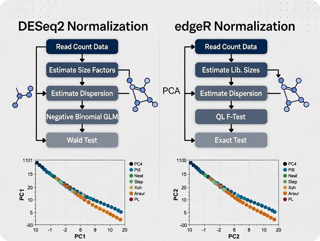
In RNA-seq analysis, normalization is an essential preprocessing step that accounts for technical variations, enabling meaningful biological comparisons between samples. Both DESeq2 and edgeR, two widely used Bioconductor packages for differential expression analysis, require careful data preparation to function optimally [19] [29]. While they share similarities in processing raw count data, their underlying normalization methodologies differ significantly, which can impact downstream analyses such as Principal Component Analysis (PCA) [10] [30].
The fundamental challenge in RNA-seq normalization stems from technical variations including sequencing depth, RNA composition, and library preparation protocols [19] [31]. These technical factors can obscure biological signals if not properly accounted for. DESeq2 employs a median-of-ratios approach, whereas edgeR utilizes the trimmed mean of M-values (TMM) method [32]. Both methods operate under the core assumption that most genes are not differentially expressed, though they implement this assumption through different statistical frameworks [19] [30].
This guide provides a comprehensive comparison of data preparation workflows for DESeq2 and edgeR, with particular emphasis on constructing count matrices and target files—the foundational inputs for both tools. We present experimental data comparing their normalization performance and provide detailed protocols for implementing these methods in practice.
Normalization Methods: Core Algorithmic Differences
DESeq2's Median-of-Ratios Method
DESeq2 employs a size factor estimation approach based on the median-of-ratios method [32] [30]. This technique calculates normalization factors by comparing each gene's count to a pseudo-reference sample derived from geometric means across all samples.
The key steps in DESeq2's normalization include:
- Geometric mean calculation: For each gene, compute the geometric mean across all samples
- Ratio computation: For each sample and each gene, compute the ratio of the gene's count to the geometric mean
- Size factor determination: The median of these ratios for each sample serves as the size factor
This method is particularly robust to differential expression in a subset of genes, as the median is resistant to outliers [30]. DESeq2 incorporates these size factors into its generalized linear model (GLM) framework, using them as offsets in the negative binomial regression [30].
edgeR's Trimmed Mean of M-values (TMM)
edgeR implements the TMM normalization procedure, which operates by selecting a reference sample and then calculating scaling factors for all other samples relative to this reference [32]. The method focuses on genes that are not differentially expressed and exhibit moderate expression levels.
The TMM algorithm involves:
- Reference selection: Typically the sample whose upper quartile is closest to the mean upper quartile across all samples
- M-value calculation: For each non-reference sample, compute log-fold changes (M-values) relative to the reference
- A-value calculation: Compute the average intensity (A-values) for each gene
- Trimming: Remove genes with extreme M-values and extreme A-values (typically top and bottom 30%)
- Scaling factor computation: Calculate the weighted mean of M-values for remaining genes
TMM normalization effectively accounts for RNA composition biases, which occur when a small subset of genes is highly expressed in one condition, potentially distorting the apparent expression of other genes [19].
Table 1: Core Normalization Algorithms in DESeq2 and edgeR
| Aspect | DESeq2 | edgeR |
|---|---|---|
| Method Name | Median-of-ratios | Trimmed Mean of M-values (TMM) |
| Key Reference | Geometric mean across samples | Single reference sample |
| Statistical Basis | Median ratios | Weighted mean of log-ratios |
| Trim Parameters | None (uses median) | Typically 30% trim each tail |
| Handling of DE Genes | Robust due to median | Robust due to trimming and weighting |
| Implementation in Package | estimateSizeFactors() |
calcNormFactors() |
Data Preparation Fundamentals
Count Matrix Construction
The foundational input for both DESeq2 and edgeR is a count matrix containing raw read counts for features (genes or transcripts) across all samples [29] [33]. This matrix should be constructed with genes as rows and samples as columns, containing integer values representing the number of reads mapped to each feature.
Proper count matrix construction requires:
- Raw count data: Avoid normalized counts (e.g., RPKM, FPKM) as input
- Feature consistency: Consistent gene identifiers across all samples
- Complete data: No missing values in the matrix
Count data can be generated using various alignment and quantification tools such as HTSeq, featureCounts, or Salmon, with the output typically consisting of separate count files for each sample [29] [33].
Target File Specification
The target file (also called sample metadata or colData) provides essential experimental design information that enables proper statistical modeling [29]. This tab-separated file should include:
Table 2: Essential Target File Components
| Column Name | Description | Example Content | Requirement |
|---|---|---|---|
| sampleName | Unique identifier for each sample | WT1, WT2, KO1, KO2 | Mandatory |
| fileName | Name of the count file for the sample | WT1counts.txt, WT2counts.txt | Mandatory |
| condition | Primary experimental factor | Control, Treated | Mandatory |
| batch | Batch effect factor (if applicable) | Batch1, Batch2 | Optional |
The target file enables both packages to associate count data with experimental factors, which is crucial for proper differential expression testing and accounting for batch effects [29] [10].
Figure 1: Workflow for constructing count matrices and target files from raw sequencing data
Experimental Comparison of Normalization Performance
Methodology for Normalization Assessment
To evaluate the performance of DESeq2 and edgeR normalization methods in the context of PCA, we analyzed data from a comparative study examining multiple normalization approaches [31]. The experimental design included:
- Dataset: 726 individual Drosophila melanogaster from the Drosophila Genetic Reference Panel
- Factors: Genotype, environment, sex, and their interactions
- Replicates: 8 biological replicates per genotype, environment, and sex combination
- Normalization Methods: Total Count (TC), Upper Quartile (UQ), Median (Med), TMM (edgeR), DESeq, Quantile (Q), RPKM, and RUVg
- Evaluation Metrics: Data alignment across samples, dynamic range preservation, and impact on differential expression results
The performance assessment focused on each method's ability to properly align data distributions across samples while preserving biological signals, particularly important for dimensionality reduction techniques like PCA [31] [10].
Comparative Performance Results
Table 3: Normalization Method Performance Comparison
| Normalization Method | Data Alignment | Dynamic Range | DE Result Quality | Sensitivity to Filtering |
|---|---|---|---|---|
| DESeq | Excellent | Excellent | High | Low |
| TMM (edgeR) | Excellent | Excellent | High | High |
| Median | Good | Good | Medium | High |
| Upper Quartile | Good | Good | Medium | Medium |
| Total Count | Poor | Poor | Low | Low |
| Quantile | Poor | Poor | Low | Medium |
| RPKM | Poor | Poor | Low | Low |
The comparative analysis revealed that both DESeq and TMM normalization methods effectively aligned data distributions across samples and accounted for the dynamic range of the data [31]. However, TMM demonstrated higher sensitivity to the filtering strategy employed, particularly the removal of low-expressed genes from the dataset.
In the context of PCA applications, both DESeq2 and edgeR normalization methods produced similar results with real datasets, though differences emerged in more complex experimental designs [9] [10]. The choice between methods should consider whether the experimental conditions might induce global shifts in expression, as such scenarios can differentially impact the normalization approaches [19].
Practical Implementation Protocols
DESeq2-Specific Workflow
Implementing DESeq2 requires specific steps for data preparation and normalization:
Figure 2: DESeq2 analysis workflow from count matrix to normalized data
Code Implementation:
edgeR-Specific Workflow
The edgeR workflow differs in its normalization approach:
Figure 3: edgeR analysis workflow from count matrix to normalized data
Code Implementation:
The Scientist's Toolkit: Essential Research Reagents
Table 4: Essential Tools and Resources for RNA-seq Data Preparation
| Tool/Resource | Function | Application in DESeq2/edgeR |
|---|---|---|
| HTSeq | Read counting against genomic features | Generate count matrices from BAM files |
| featureCounts | Efficient read counting | Generate count matrices from BAM files |
| tximport | Transcript-level quantification | Import transcript abundance to gene-level counts |
| DESeq2 Package | Differential expression analysis | Normalization and statistical testing |
| edgeR Package | Differential expression analysis | Normalization and statistical testing |
| SARTools Pipeline | Automated RNA-seq analysis | Standardized workflow for both DESeq2 and edgeR |
| Galaxy Platform | Web-based bioinformatics | User-friendly interface for RNA-seq analysis |
| BeCorrect Tool | Batch effect correction | Address unwanted variation in count data |
Impact of Normalization on PCA Results
The choice of normalization method significantly influences PCA outcomes, which is particularly relevant for exploratory data analysis and quality assessment [10] [34]. Proper normalization ensures that technical variance doesn't dominate biological variance in the principal components.
Key considerations for PCA applications:
- Variance stabilization: Both DESeq2 and edgeR offer transformations (rlog/VST for DESeq2, log-CPM for edgeR) that stabilize variance across the mean expression range
- Batch effects: If present in the experimental design, batch effects should be incorporated in the normalization model
- Sample separation: The first principal components should ideally separate samples by biological conditions of interest rather than technical factors
Studies have shown that while DESeq2 and edgeR normalization methods generally produce similar PCA patterns with well-behaved data, differences can emerge in datasets with extreme composition biases or global expression shifts [19] [31]. Researchers should perform PCA as a quality control step regardless of their chosen normalization method to identify potential outliers or unexpected sample groupings.
Data preparation—specifically the construction of proper count matrices and target files—forms the critical foundation for successful RNA-seq analysis with both DESeq2 and edgeR. While both tools require similar input data structures, their normalization approaches differ fundamentally: DESeq2 employs a median-of-ratios method, whereas edgeR utilizes the trimmed mean of M-values.
Experimental evidence indicates that both normalization methods perform well in typical RNA-seq datasets, effectively aligning data distributions across samples and preserving biological signals for downstream analyses including PCA. DESeq's method demonstrates slightly lower sensitivity to filtering strategies, while TMM normalization shows robust performance across diverse experimental conditions.
For researchers implementing these tools, we recommend careful attention to:
- Using raw count data rather than pre-normalized values
- Including comprehensive sample metadata in target files
- Performing quality control checks (including PCA) after normalization
- Considering experimental design complexity when choosing between methods
By following the detailed protocols and considerations outlined in this guide, researchers can ensure that their data preparation provides optimal foundation for both DESeq2 and edgeR analyses, leading to more reliable and interpretable results in their transcriptomic studies.
Principal Component Analysis (PCA) is an essential exploratory tool in bulk RNA-sequencing data analysis, providing researchers with a visual assessment of sample similarity and overall data structure. By reducing the dimensionality of complex gene expression datasets, PCA plots reveal inherent clustering patterns, potential batch effects, and outliers that might influence downstream interpretation. The choice of data transformation method applied prior to PCA significantly impacts these visualizations, making the selection between Variance Stabilizing Transformation (VST) from DESeq2 and alternative normalization methods a critical methodological decision. Within the broader context of comparing DESeq2 versus edgeR normalization for PCA research, this guide objectively evaluates the performance of DESeq2's VST against other common approaches, providing experimental data and protocols to inform researchers in pharmaceutical development and basic research.
The fundamental challenge in RNA-seq PCA generation stems from count data heterogeneity, where the variance of counts depends strongly on their mean. This heteroskedasticity violates assumptions underlying standard statistical methods used in PCA, necessitating specialized transformations that stabilize variance across the dynamic range of expression values. DESeq2's VST directly addresses this challenge by incorporating a gamma-Poisson distribution model that accounts for overdispersion in count data, while edgeR's traditional approach utilizes a logarithmic transformation of counts per million (CPM) with precision weighting. Understanding the technical nuances and performance characteristics of these competing approaches enables researchers to make informed analytical decisions that enhance the reliability of their exploratory findings.
Comparative Performance Analysis
Methodological Differences and Theoretical Basis
The core distinction between DESeq2's VST and edgeR's log-CPM approach lies in their theoretical foundations for handling RNA-seq count distributions. DESeq2's VST employs a parametric transformation derived from the fitted dispersion-mean relationship, explicitly modeling the mean-variance dependence characteristic of count data. This approach combines the benefits of variance stabilization with a generalized linear model framework that accounts for experimental design factors. In contrast, edgeR's standard PCA pipeline utilizes a non-parametric transformation through log-CPM values with TMM (Trimmed Mean of M-values) normalization, which corrects for composition biases between samples but applies a generic variance stabilization approach.
Research indicates that the VST method in DESeq2 is specifically designed to counteract heteroskedasticity by yielding transformed data where the variance remains approximately constant throughout the dynamic range of expression values. This property is particularly valuable for PCA, as it ensures that both highly and lowly expressed genes contribute more equally to principal component calculations without being dominated by technical variance patterns. Meanwhile, edgeR's log-CPM approach with precision weights (voom transformation) adjusts for mean-variance relationships through non-parametric smoothing, offering an alternative solution to the same fundamental challenge. Benchmarks using real and simulated data suggest that while both methods perform similarly in many scenarios, VST may demonstrate advantages in datasets with extreme overdispersion or when the experimental design incorporates multiple factors that need simultaneous consideration.
Quantitative Performance Comparison
Table 1: Comparative Performance of Transformation Methods for PCA in RNA-Seq Analysis
| Performance Metric | DESeq2 VST | edgeR log-CPM | limma-voom |
|---|---|---|---|
| Variance Stabilization | Explicit parametric modeling of mean-variance relationship | Non-parametric approach with TMM normalization | Precision weights based on mean-variance trend |
| Handling of Low Counts | Automatic filtering; shrinkage of LFC estimates | Requires manual filtering; can produce extreme LFC in low counts | Benefits from pre-filtering; voom provides precision weights |
| Computational Efficiency | Moderate efficiency for small to medium datasets | Fast processing speed | Highly efficient, especially for large datasets |
| Batch Effect Management | Can incorporate batch terms in design formula | Similar capability through design matrix | Excellent handling of complex designs and batch effects |
| Sample Size Recommendation | Performs well with ≥3 replicates per condition | Efficient with very small sample sizes (n≥2) | Optimal with ≥3 replicates per condition |
| Key Advantage | Integrated normalization and transformation pipeline | Speed and flexibility in dispersion estimation | Superior handling of complex experimental designs |
Table 2: Practical Implementation Considerations for PCA Workflows
| Implementation Factor | DESeq2 VST Workflow | edgeR log-CPM Workflow |
|---|---|---|
| Default Gene Selection | Uses top 500 most variable genes | No inherent gene filtering in plotMDS |
| Data Scaling | No additional scaling recommended | Scaling not recommended in standard pipeline |
| Required Preprocessing | Independent filtering of low counts | filterByExpr() for low counts; calcNormFactors() |
| Visualization Function | plotPCA() integrated in DESeq2 | plotMDS() in edgeR |
| Integration with DE Analysis | Seamless with DESeq2 DE pipeline | Direct integration with edgeR DE analysis |
Empirical comparisons between these transformation approaches reveal nuanced performance differences. A critical benchmark study noted that when PCA results appear substantially different between methods, the discrepancy often stems more from implementation details than fundamental algorithmic superiority. Specifically, the default settings for each method vary significantly—DESeq2's plotPCA() function automatically uses the top 500 most variable genes, while edgeR's plotMDS() typically utilizes all genes passing expression filters. Similarly, the application of data scaling (e.g., scale.=TRUE in prcomp) dramatically impacts PCA visualizations, with experts generally recommending against scaling when working with log-CPM or VST-transformed data, as these transformations already address the heteroskedasticity that scaling would otherwise mitigate [35].
Experimental data from systematic comparisons indicate that when implementation inconsistencies are eliminated, VST and log-CPM transformations typically produce similar PCA clustering patterns for well-behaved datasets. However, in cases with pronounced batch effects or substantial differences in library sizes, VST may demonstrate superior performance in separating biological signal from technical artifacts. One study observed that VST better handles size factor variations across samples, preventing the artificial separation of samples based solely on sequencing depth rather than biological meaningful differences [36]. This characteristic makes DESeq2's VST particularly valuable in clinical and pharmaceutical research settings, where samples may be processed in multiple batches across time.
Experimental Protocols
DESeq2 VST PCA Workflow
The following protocol details the complete procedure for generating PCA plots from raw count data using DESeq2's Variance Stabilizing Transformation:
Step 1: Data Preparation and Preprocessing Begin by importing raw count data into a DESeqDataSet object, simultaneously incorporating sample metadata and experimental design information. Filter out lowly expressed genes that might introduce noise, as these can disproportionately influence PCA results. While DESeq2 performs some automatic filtering, proactive removal of genes with minimal expression across samples enhances overall signal-to-noise ratio.
Step 2: Variance Stabilizing Transformation
Apply the VST to the filtered DESeqDataSet. Set blind=FALSE to ensure the transformation considers the experimental design, which is particularly important when expecting strong batch effects or when the experimental design includes multiple factors.
Step 3: PCA Visualization Generate the PCA plot using DESeq2's integrated plotPCA() function, specifying the primary experimental condition for color coding. The function automatically selects the 500 genes with highest variance across samples, providing an optimal balance between signal capture and computational efficiency.
For enhanced customization or when incorporating additional aesthetic elements, manually extract the VST-transformed values and utilize standard plotting functions:
edgeR log-CPM PCA Workflow
For comparative purposes, the following protocol outlines the standard edgeR approach to PCA visualization:
Step 1: Data Preprocessing and Normalization Create a DGEList object containing count data and sample information, then apply filtering based on expression levels across samples. Normalize library sizes using the TMM method to correct for composition biases.
Step 2: Transformation and PCA Generation Compute log-CPM values and generate multidimensional scaling (MDS) plot, which represents edgeR's analogous approach to PCA visualization.
Alternatively, for direct comparison with DESeq2 output, perform conventional PCA on the log-CPM values:
Workflow Visualization
Diagram 1: Comparative workflow for PCA generation using DESeq2 VST versus edgeR log-CPM approaches
The Scientist's Toolkit
Table 3: Essential Research Reagent Solutions for RNA-Seq PCA Analysis
| Tool/Reagent | Function in PCA Workflow | Implementation Notes |
|---|---|---|
| DESeq2 R Package | Provides VST transformation and integrated PCA visualization | Critical for DESeq2 workflow; enables seamless transition to DE analysis |
| edgeR R Package | Offers log-CPM transformation and MDS plotting capabilities | Optimal for users already committed to edgeR DE pipeline |
| limma R Package | Alternative approach with voom transformation for RNA-seq data | Particularly effective for complex experimental designs |
| filterByExpr() Function | Automated filtering of lowly expressed genes in edgeR | Reduces noise from minimally expressed transcripts |
| TMM Normalization | Composition bias correction in edgeR pipeline | Accounts for RNA production differences between samples |
| RLE Normalization | DESeq2's default size factor estimation | Corrects for library size differences using geometric means |
| plotPCA() Function | DESeq2's integrated PCA visualization tool | Automatically uses top 500 variable genes; customizable |
| plotMDS() Function | edgeR's multidimensional scaling visualization | edgeR's equivalent to PCA; based on pairwise distances |
Interpretation Guidelines
Interpreting PCA plots generated from VST-transformed data requires attention to several critical factors that distinguish them from visualizations based on alternative transformations. First, assess the percentage of variance explained by each principal component, which indicates the relative strength of the separation patterns observed. When biological conditions separate clearly along PC1, this suggests strong transcriptional signatures associated with the experimental variable. However, when technical factors such as batch processing or library preparation date drive primary separation patterns, this may indicate the need for additional covariate adjustment in the experimental design.
Research demonstrates that VST-based PCA plots typically show reduced technical artifact amplification compared to log-CPM transformations, particularly in datasets with wide variations in sequencing depth. This property makes VST particularly valuable for detecting subtle biological signals in the presence of substantial technical noise. However, users should remain aware that the default selection of the top 500 variable genes in DESeq2's plotPCA() function may emphasize different aspects of the data compared to edgeR's approach of utilizing all expressed genes. This methodological difference can explain apparent discrepancies when comparing results across platforms, even when analyzing identical datasets [35].
For robust interpretation, researchers should correlate PCA findings with other quality metrics and exploratory visualizations. Specifically, strong separation between biological replicates of the same condition may indicate uncontrolled technical variation or inadequate normalization. Conversely, tight clustering of replicate samples with clear separation between conditions provides confidence in both data quality and the strength of biological effects. When using VST transformation, particularly note whether the assumed mean-variance relationship adequately fits the data, as poor fit can diminish the effectiveness of variance stabilization and potentially distort PCA interpretations.
DESeq2's Variance Stabilizing Transformation provides a robust foundation for PCA visualization in RNA-seq studies, offering theoretically sound handling of count data heteroskedasticity through its parametric framework. Comparative analysis reveals that while VST and edgeR's log-CPM approaches typically yield similar clustering patterns for standard datasets, VST may demonstrate advantages in studies with pronounced technical variability or complex experimental designs. The integrated nature of the DESeq2 pipeline—from normalization through transformation to differential expression analysis—offers practical benefits for researchers seeking a unified analytical workflow.
The choice between these transformation methods should be guided by specific research contexts and data characteristics. For projects already committed to the DESeq2 ecosystem for differential expression analysis, leveraging VST for exploratory visualization provides methodological consistency throughout the analytical pipeline. Conversely, when working within the edgeR framework or analyzing exceptionally large datasets where computational efficiency is paramount, the log-CPM approach remains a competitive alternative. Regardless of the selected method, maintaining consistency in implementation parameters—particularly regarding gene selection, filtering thresholds, and scaling options—is essential for generating biologically meaningful and technically reproducible PCA visualizations that accurately reflect the underlying transcriptomic landscape.
In the analysis of RNA-sequencing (RNA-seq) data, Principal Component Analysis (PCA) is a fundamental exploratory tool used to visualize global gene expression patterns, identify sample outliers, and assess batch effects. The validity of these visualizations is profoundly influenced by the chosen normalization method, which accounts for technical variations like sequencing depth and RNA composition. Within the broader thesis comparing DESeq2 and edgeR normalization strategies for PCA, this guide focuses specifically on implementing a robust PCA workflow using edgeR's log-counts-per-million (log-CPM) values stabilized with the Trimmed Mean of M-values (TMM) factors. We objectively compare its performance against alternative methods, providing experimental data and detailed protocols to guide researchers in making informed analytical decisions [8] [37].
Core Normalization Concepts for PCA
Before detailing the workflow, it is essential to understand the normalization principles that underpin a reliable PCA.
- Sequencing Depth: Samples are sequenced to different depths, leading to varying total numbers of reads. Normalization adjusts for this to prevent samples from appearing different based purely on their library size [37].
- RNA Composition: A few highly differentially expressed genes or differences in the number of expressed genes between samples can skew counts. Methods like TMM are designed to be robust to such composition biases [37].
- The Role of TMM: The Trimmed Mean of M-values (TMM) method, implemented in
edgeR, calculates scaling factors between samples by using a weighted trimmed mean of log-expression ratios (M-values). It assumes that the majority of genes are not differentially expressed, making it robust to imbalances in RNA composition that can occur when comparing different tissues or conditions [8] [37]. For PCA, TMM normalization is particularly valuable as it helps to ensure that the major sources of variation captured in the principal components reflect biological differences rather than technical artifacts [4].
It is critical to note that TMM normalizes the effective library sizes, not the counts directly. The resulting normalized expression values, used for visualization in PCA, are typically generated as log-CPM values [16].
Experimental Protocol: PCA from edgeR's TMM log-CPM
This section provides a step-by-step protocol for generating a PCA plot from an RNA-seq count matrix using edgeR. The following workflow diagram outlines the entire process.
Workflow Diagram
Step-by-Step Methodology
Load Required Libraries and Data: Begin by installing and loading the necessary R packages. Then, read your raw count matrix and sample metadata. The count matrix should be a table where rows are genes and columns are samples [13].
Create DGEList Object and Filter Genes: The
DGEListobject is the standard data structure inedgeR. After creating it, filter out genes with very low counts across samples, as they contribute mostly noise to the PCA [13] [38].Calculate TMM Normalization Factors: This crucial step computes the scaling factors that correct for differences in sequencing depth and RNA composition between samples. The
calcNormFactorsfunction does not change the counts but stores the factors within theDGEListobject for subsequent steps [16].Generate log-Transformed CPM Values: Use the
cpmfunction with thelog=TRUEargument to compute log₂-CPM values. These values are normalized using the effective library sizes (original library sizes adjusted by the TMM factors). The log transformation stabilizes the variance, making the data more suitable for PCA [16].Perform PCA and Visualize Results: Conduct PCA on the transposed
log_cpm_matrix(so that samples are rows and genes are columns). Theprcompfunction is used here, and the results are visualized in a scatter plot of the first two principal components.
Performance Comparison with Alternative Methods
To objectively evaluate the edgeR TMM workflow, we compare its performance against other common normalization approaches using both published experimental data and benchmark studies. The table below summarizes quantitative comparisons from a real RNA-seq dataset (tomato fruit set, 9 samples, 3 conditions) [8].
Table 1: Comparison of Normalization Factors from a Tomato Fruit Set Dataset [8]
| Sample | TMM Factors | RLE (DESeq2) Factors | MRN Factors |
|---|---|---|---|
| Bud 1 | 0.980 | 1.017 | 0.871 |
| Bud 2 | 0.922 | 0.809 | 0.754 |
| Bud 3 | 0.720 | 0.727 | 0.914 |
| Ant 1 | 1.058 | 0.866 | 0.793 |
| Ant 2 | 0.981 | 1.236 | 1.201 |
| Ant 3 | 0.884 | 0.736 | 0.805 |
| Pos 1 | 1.130 | 1.282 | 1.340 |
| Pos 2 | 1.194 | 1.272 | 1.253 |
| Pos 3 | 1.241 | 1.373 | 1.293 |
The data shows that while TMM, RLE, and MRN methods do not yield identical factors, RLE and MRN factors are often closer to each other. A key differentiator is their relationship with library size: TMM factors show an "almost horizontal regression line" when plotted against library size, indicating it effectively corrects for this technical variable. In contrast, RLE and MRN factors maintain a positive correlation with library size [8].
Table 2: Summary of Benchmark Conclusions from Multiple Studies [39]
| References | Normalization Methods Compared | Key Conclusions for Differential Expression & PCA |
|---|---|---|
| Dillies et al. 2013 | DESeq, TMM, UQ, etc. | Exact test from DESeq combined with DESeq/TMM normalization performed best in controlling FDR. RPKM and TC methods were not recommended. |
| Soneson et al. 2013 | DESeq, TMM, voom, etc. | limma-voom demonstrated good FDR control. DESeq had poor FDR control with 2 samples but improved with larger sample sizes. |
| Costa-Silva et al. 2017 | TMM, RLE, UQ, voom | Limma-voom, NOIseq and DESeq2 produced the most consistent results for DEG identification, which impacts the genes driving PCA. |
| Maza E 2016 | TMM, RLE, MRN | TMM, RLE, and MRN gave identical results for a simple two-condition comparison without replicates, suggesting potential equivalence in simple designs. |
| Spies et al. 2019 | RLE, TMM, Med, etc. | For short time courses, DESeq2 and edgeR with pairwise comparisons outperformed many dedicated time-course tools. |
Comparative Interpretation
- edgeR's TMM: Consistently ranks as a robust and recommended method. It is particularly strong in handling datasets with different RNA compositions, such as when comparing different tissues or conditions where a few highly expressed genes could dominate the total library [37]. For PCA, this means TMM is less likely to allow technical composition biases to become the primary drivers of the principal components [4].
- DESeq2's RLE: Similar to TMM in its fundamental assumption (most genes are not DE), it uses the geometric mean to calculate size factors. Benchmark studies often place DESeq2 and edgeR in a similar performance tier, with DESeq2 sometimes noted for being a more "conservative" choice with strong false discovery rate (FDR) control [39] [40].
- Limma-Voom: This method involves transforming counts into log-CPM values, calculating precision weights with the
voomfunction, and then applying linear models. It is highly efficient and excels in complex experimental designs.limma-voomhas been shown to have good FDR control and stable performance, making it a strong alternative for both differential expression and the underlying data used for PCA [13] [39].
A critical consideration for PCA is that methods like RPKM, FPKM, and TPM are not designed for differential expression analysis and should not be used as input for a PCA that aims to find biologically differential samples. These methods are suited for within-sample comparisons but can introduce biases in between-sample analyses [37].
The Scientist's Toolkit
Table 3: Essential Research Reagent Solutions for RNA-seq Analysis
| Item | Function in Workflow |
|---|---|
| edgeR (R Package) | A comprehensive package for the analysis of RNA-seq data. It performs data normalization (TMM), dispersion estimation, and differential expression testing [8] [13]. |
| DESeq2 (R Package) | An alternative method for RNA-seq analysis that uses a median ratio (RLE) approach for normalization and employs an empirical Bayes approach for shrinkage of dispersion and fold-change estimates [8] [40]. |
| Limma (R Package) | A versatile package for analyzing microarray and RNA-seq data. When combined with the voom transformation, it provides a robust framework for linear modeling of count data [13] [39]. |
| R/Bioconductor Environment | The open-source computing infrastructure within which these tools are developed and operated. It provides essential data structures and functions for handling high-throughput genomic data [8] [38]. |
| Count Matrix | The fundamental input data, a table of integer counts where rows represent genomic features (e.g., genes) and columns represent sequencing libraries (samples) [38]. |
| Sample Metadata | A table describing the experimental design, linking each sample (column in the count matrix) to its experimental conditions (e.g., treatment, time point, genotype). This is crucial for coloring and interpreting PCA plots [38]. |
The workflow for creating PCA plots from edgeR's log-CPM values with TMM factors provides a robust and well-supported method for the exploratory analysis of RNA-seq data. The TMM normalization is explicitly designed to handle technical variations like sequencing depth and RNA composition, which helps ensure that the major patterns revealed by PCA are biologically meaningful. Performance comparisons show that TMM is consistently a top-performing method, on par with DESeq2's RLE normalization, though their results are not identical. The choice between edgeR-TMM, DESeq2-RLE, or limma-voom may depend on specific dataset characteristics and the analytical goal. However, the edgeR TMM workflow remains a powerful and reliable choice for researchers seeking to visualize and interpret the global structure of their gene expression data.
Differential expression analysis represents a fundamental step in understanding how genes respond to different biological conditions using RNA sequencing data. In this comparative guide, we explore two of the most widely-used tools for RNA-seq analysis: DESeq2 and edgeR. Both methods address the specific challenges of RNA-seq data, particularly count data overdispersion and small sample sizes, through sophisticated statistical approaches based on the negative binomial distribution [41] [13]. While they share this common foundation, they differ in their implementation details, normalization strategies, and analytical outputs, which can significantly impact the results of exploratory analyses such as Principal Component Analysis (PCA).
PCA serves as a crucial visualization technique for assessing sample similarity, identifying batch effects, and understanding overall data structure before formal differential expression testing [41] [42]. The normalization approaches employed by DESeq2 and edgeR directly influence the PCA results, making it essential to understand their underlying methodologies. This guide provides a comprehensive, side-by-side comparison of the complete analytical workflows for both tools, with particular emphasis on their PCA capabilities within the context of RNA-seq data normalization.
Table: Overview of DESeq2 and edgeR Characteristics
| Aspect | DESeq2 | edgeR |
|---|---|---|
| Core Statistical Approach | Negative binomial modeling with empirical Bayes shrinkage | Negative binomial modeling with flexible dispersion estimation |
| Default Normalization | Internal normalization based on geometric mean | TMM (Trimmed Mean of M-values) normalization |
| Dispersion Estimation | Adaptive shrinkage for dispersion estimates | Common, trended, or tagwise dispersion options |
| Ideal Sample Size | ≥3 replicates, performs well with more | ≥2 replicates, efficient with small samples |
| Computational Efficiency | Can be computationally intensive for large datasets | Highly efficient, fast processing |
Experimental Design and Data Preparation
For this comparison, we utilize a publicly available RNA-seq dataset to ensure reproducibility and transparency. The Pasilla dataset from an experiment in Drosophila melanogaster investigating the effect of RNAi knockdown of the splicing factor pasilla serves as our primary example [41]. This dataset includes both treated and untreated samples across different library types (single-end and paired-end), providing a realistic scenario for methodological comparison. Alternatively, the human airway smooth muscle cell dataset with dexamethasone treatment offers another well-characterized option [42] [43]. These datasets exemplify typical experimental designs in transcriptomics with multiple biological replicates across conditions, which is essential for robust differential expression analysis.
Essential Research Reagents and Computational Tools
Table: Key Research Reagent Solutions for RNA-seq Analysis
| Item | Function | Example/Note |
|---|---|---|
| RNA-seq Count Data | Raw input data for differential expression analysis | Integer counts of reads per gene [42] |
| Sample Metadata | Experimental design specification | Condition, batch, library type information [44] |
| DESeq2 R Package | Differential expression analysis | Provides normalization, dispersion estimation, and testing [33] [44] |
| edgeR R Package | Differential expression analysis | Offers TMM normalization and flexible dispersion modeling [41] [13] |
| Bioconductor | Repository for bioinformatics packages | Installation source for both DESeq2 and edgeR [44] |
| Annotation Files | Gene model information | GTF/GFF files for read counting [42] |
Workflow Diagram for RNA-seq Analysis
Methodology: Side-by-Side R Scripts
Data Preparation and Import
Both DESeq2 and edgeR require the same fundamental data inputs: a count matrix of raw integer counts (not normalized values) and a sample metadata table describing the experimental design [42]. The count values must be raw counts of sequencing reads, as only actual counts allow proper assessment of measurement precision for the statistical models employed by both methods [42].
DESeq2 Data Preparation Code:
edgeR Data Preparation Code:
Normalization and Dispersion Estimation
The normalization approaches represent a fundamental difference between DESeq2 and edgeR. DESeq2 uses a median-of-ratios method based on the geometric mean of counts, while edgeR employs the TMM (Trimmed Mean of M-values) method [13]. Both approaches effectively correct for library size differences and RNA composition biases, but their mathematical foundations differ, potentially leading to variations in downstream analyses including PCA.
DESeq2 Normalization and Analysis Code:
edgeR Normalization and Analysis Code:
PCA and Data Visualization
Visualization of sample relationships through dimensionality reduction is critical for quality assessment and exploratory analysis. DESeq2 provides built-in PCA functionality, while edgeR offers MDS (Multi-Dimensional Scaling) plots, which serve a similar purpose though with different mathematical foundations [41].
DESeq2 PCA Visualization Code:
edgeR Visualization Code:
Comparative Analysis of Results
Normalization Differences and Impact on PCA
The normalization approaches employed by DESeq2 and edgeR, while both effective, can lead to different visual patterns in dimensionality reduction plots. DESeq2's median-of-ratios method tends to be more robust to extreme count values, while edgeR's TMM method provides excellent performance across diverse experimental conditions [13].
Table: Comparison of Normalization Approaches
| Normalization Aspect | DESeq2 | edgeR |
|---|---|---|
| Method Name | Median-of-ratios | TMM (Trimmed Mean of M-values) |
| Core Concept | Geometric mean-based size factors | Weighted trimmed mean of log expression ratios |
| Handling of Extreme Values | Robust due to geometric mean | Uses trimming to exclude extreme genes |
| Dispersion Estimation | Empirical Bayes shrinkage | Common, trended, or tagwise dispersion |
| Impact on PCA | Can be more conservative for low counts | May show clearer separation with large fold changes |
Performance Comparison and Benchmarking
Several benchmark studies have evaluated the performance of DESeq2 and edgeR across various experimental conditions. In practice, both tools perform admirably, with subtle differences in specific scenarios [13]. DESeq2 demonstrates particular strength in handling experiments with moderate to large sample sizes and high biological variability, while edgeR excels with very small sample sizes and datasets containing many low-abundance transcripts [13].
Concordance in Results
Despite their methodological differences, DESeq2 and edgeR typically show substantial agreement in identifying differentially expressed genes. One comparative analysis noted that edgeR often identifies a larger number of significant genes, though this doesn't necessarily indicate superior performance, as it might include more false positives without proper filtering [41]. Both packages provide mechanisms for independent filtering to remove low-count genes that lack statistical power for differential expression detection.
Code for Comparing Results:
Best Practices and Recommendations
Experimental Design Considerations
Proper experimental design is crucial for obtaining meaningful results from RNA-seq analysis. Both DESeq2 and edgeR require biological replicates to estimate variability reliably. For simple two-group comparisons with balanced designs, both tools perform excellently, but for more complex designs involving multiple factors, batch effects, or time courses, careful specification of the design matrix is essential [45].
Handling Batch Effects:
Troubleshooting Common Issues
RNA-seq analysis often presents challenges such as poor sample clustering in PCA, low number of differentially expressed genes, or normalization problems. Both DESeq2 and edgeR provide diagnostic plots to identify potential issues.
Diagnostic Code for DESeq2:
Diagnostic Code for edgeR:
Tool Selection Guidelines
The choice between DESeq2 and edgeR depends on multiple factors, including sample size, experimental complexity, and specific research questions [13].
Table: Guidelines for Tool Selection
| Scenario | Recommended Tool | Rationale |
|---|---|---|
| Very small sample sizes (n < 5) | edgeR | More efficient with limited replicates |
| Complex experimental designs | DESeq2 or edgeR (with limma) | Both handle complex designs well |
| Large datasets (>100 samples) | edgeR | Better computational efficiency |
| Focus on low-abundance transcripts | edgeR | Superior handling of low counts |
| Emphasis on conservative results | DESeq2 | Tends to be more conservative |
| Integration with other omics data | DESeq2 or limma | Easier integration workflows |
DESeq2 and edgeR represent two sophisticated, well-validated approaches for differential expression analysis and visualization in RNA-seq experiments. While both utilize negative binomial distributions and address similar analytical challenges, their implementation details, normalization strategies, and visualization approaches differ in ways that can impact PCA results and biological interpretation.
DESeq2's median-of-ratios normalization and more conservative approach often makes it preferable for studies emphasizing robust, conservative findings with moderate to large sample sizes. edgeR's TMM normalization and efficient computation makes it excellent for studies with limited samples, large datasets, or particular interest in low-abundance transcripts.
For most standard RNA-seq analyses, both tools provide reliable, reproducible results, and the choice between them may come down to researcher familiarity, specific experimental constraints, or institutional preferences. Regardless of the chosen tool, proper experimental design with adequate biological replicates, careful quality control, and appropriate interpretation of PCA and other diagnostic plots remain essential for generating biologically meaningful insights from RNA-seq data.
Integrating Normalization into Automated Pipelines (e.g., SARTools)
Normalization of RNA-sequencing (RNA-seq) data is a critical preprocessing step that corrects for technical variations, such as differences in library sizes and sequencing depth, to enable accurate biological comparisons. The choice of normalization method can profoundly influence downstream analyses, including principal component analysis (PCA) and the detection of differentially expressed (DE) genes [4]. However, properly implementing normalization within statistical frameworks requires considerable expertise and can be a source of errors for untrained users.
SARTools (Statistical Analysis of RNA-Seq data Tools) is an R pipeline designed to address these challenges by providing a structured, reproducible environment for the differential analysis of RNA-seq count data [29] [46]. It integrates two of the most popular Bioconductor packages for this purpose, DESeq2 and edgeR, and automates their respective normalization procedures within a comprehensive workflow. This guide objectively compares how SARTools incorporates and implements the distinct normalization methodologies of DESeq2 and edgeR, examining their impact on exploratory analyses like PCA and providing supporting experimental data from independent evaluations.
SARTools Pipeline: Architecture and Workflow
SARTools is structured as an R package accompanied by two R script templates—one for DESeq2 and one for edgeR [29] [47]. Its primary function is to guide users through a complete analysis, from reading raw count data to generating a final HTML report, while enforcing essential quality control (QC) steps that might otherwise be overlooked.
Input Requirements and Design Specifications
The pipeline requires two primary inputs:
- Count Data Files: One file per sample, containing two tab-delimited columns without a header (unique feature identifier and raw feature count). HTSeq-count output files are directly compatible [29] [48].
- Target File: A tab-delimited file describing the experimental design. It must contain at least three columns with headers: sample labels, corresponding count file names, and biological conditions. An optional fourth column can specify a blocking factor (e.g., batch effect or sample pairing) [29].
SARTools handles experimental designs involving a single biological factor with two or more conditions. It can also account for a blocking factor to control for batch effects or paired samples. However, it does not support complex designs with interactions [29].
Comprehensive Workflow Visualization
The following diagram illustrates the key stages of the SARTools workflow, highlighting points where DESeq2 and edgeR-specific processes diverge, particularly during normalization.
Normalization in DESeq2 vs. edgeR: A Technical Comparison
Within the SARTools framework, the underlying normalization methods of DESeq2 and edgeR are applied as intended by their original developers. The following table provides a detailed comparison of these core normalization approaches.
Table 1: Comparison of Normalization Methods in DESeq2 and edgeR as Implemented in SARTools
| Aspect | DESeq2 | edgeR |
|---|---|---|
| Core Method | Size factors (median-of-ratios) [29] | Scaling factors (e.g., TMM - Trimmed Mean of M-values) [29] |
| Philosophy | Estimates a sample-specific size factor used directly in the parameterization of the Negative Binomial model's mean. [29] | Calculates normalized library sizes used as an offset in the statistical model. [29] |
| Model Integration | Size factors are used to model the mean of the Negative Binomial distribution. [29] | Normalized library sizes are included as an offset in the statistical model. [29] |
| Theoretical Goal | Corrects for library size and RNA composition bias, assuming most genes are not DE. [29] | Corrects for library size and RNA composition bias, assuming most genes are not DE. [29] |
| Interchangeability | Not directly interchangeable without adequate transformation. Using them incorrectly leads to inconsistent results. [29] | Not directly interchangeable without adequate transformation. Using them incorrectly leads to inconsistent results. [29] |
| Alternative Options in SARTools | fitType parameter ("parametric" or "local" for mean-dispersion relationship) [48] |
normalization parameter to select alternative methods (not specified in results) [29] |
Impact of Normalization on PCA and Exploratory Analysis
A principal goal of normalization is to prepare data for exploratory analyses like PCA. However, different normalization strategies can lead to different interpretations of the same dataset.
The Normalization-PCA Interrelationship
PCA assumes that the data are homoscedastic, meaning the variance is independent of the signal intensity. Raw RNA-seq count data violate this assumption [29]. SARTools automatically applies appropriate transformations to meet this assumption for PCA and clustering:
- When using the DESeq2 template, it employs either the Variance Stabilizing Transformation (VST) or the regularized log transformation (rlog) [29] [48].
- When using the edgeR template, it uses log Counts Per Million (CPM) values [29].
These transformations are crucial because using raw counts or Reads Per Kilobase per Million (RPKM) is unsuitable for these multivariate methods [29].
Experimental Evidence on Normalization Effects
Independent research highlights the profound impact normalization choice has on PCA outcomes. A comprehensive evaluation of 12 normalization methods found that while PCA score plots might appear similar across different methods, the biological interpretation of the models can depend heavily on the normalization method applied [4]. The study concluded that correlation patterns in the data, model complexity, and gene ranking in the PCA model fit are all significantly affected by the normalization procedure.
Furthermore, the choice between absolute counts and relative abundance is critical. Protocols using Unique Molecular Identifiers (UMIs), common in single-cell RNA-seq, allow for absolute quantification. Normalizing such data with methods like CPM, which converts data into relative abundances, can erase useful biological information. For instance, differences in total RNA content between cell types can be obscured by CPM normalization, potentially masking biologically important variation [49]. SARTools avoids this pitfall by relying on the robust, count-based normalization schemes of DESeq2 and edgeR, which are designed for relative expression analysis from raw counts.
The following diagram conceptualizes how normalization choices within a pipeline like SARTools influence the trajectory of data analysis and its final biological interpretation.
Performance Evaluation and Experimental Data
Benchmarking Insights on Differential Expression Analysis
While direct benchmarks of SARTools are limited, numerous studies have evaluated its core engines, DESeq2 and edgeR. A key finding is that despite their methodological differences, the default normalization methods in both packages "have been shown to perform equally well" in replicated experiments for differential expression analysis [29].
Large-scale benchmarking of differential expression methods, including those designed for single-cell data, reinforces the robustness of well-established bulk RNA-seq tools. A 2023 benchmark of 46 workflows for single-cell data with batch effects found that parametric methods like DESeq2 and limma-trend showed good performance, and the use of batch-covariate modeling (a feature supported by SARTools through its blocking factor) often improved analysis for large batch effects [50]. This underscores the value of SARTools' structured approach, which facilitates proper experimental design and covariate inclusion.
Diagnostic and QC Outputs from SARTools
SARTools generates a comprehensive HTML report with numerous diagnostic plots that allow researchers to assess the quality of their data and the appropriateness of the model, including the normalization [29] [48]. Key outputs related to normalization and data quality include:
- Diagnostic of Size Factors: Plots size factors versus the total number of reads to check for technical biases [48].
- Counts Boxplots: Displays boxplots of both raw and normalized counts, allowing for a visual assessment of normalization efficacy across samples [48].
- PCA Plot: Based on the properly transformed (VST/rlog or log-CPM) data, this plot helps visualize sample-to-sample distances and identify the main sources of variation in the dataset [29] [48].
- Sample Clustering: A hierarchical clustering plot of samples, also based on transformed data, provides a complementary view to the PCA [48].
These integrated diagnostics are a critical feature, as they help users avoid spurious results stemming from poor data quality or misapplied normalization, fulfilling the pipeline's goal of preventing errors from misusing DESeq2 and edgeR [29].
Practical Implementation Guide
The Researcher's Toolkit: Essential Materials and Reagents
Table 2: Key Research Reagent Solutions for Using SARTools
| Item | Function in the Workflow |
|---|---|
| R Environment (v3.3.0+) | The foundational computing platform required to run the SARTools pipeline and its dependencies [46]. |
| Bioconductor Packages | Provides the core analytical libraries: DESeq2 (v1.12.0+) and edgeR (v3.12.0+), which perform the statistical calculations [46]. |
| SARTools R Package | The automated pipeline itself, providing the wrapper functions, script templates, and reporting utilities [46]. |
| HTSeq-count or similar | An alignment and counting tool (outside SARTools scope) to generate the required raw count input files from sequence reads [29]. |
| Galaxy Wrapper (Optional) | Provides a user-friendly graphical interface to run SARTools within a Galaxy instance, increasing accessibility for biologists [29]. |
Step-by-Step Experimental Protocol
To implement a comparative analysis of DESeq2 and edgeR normalization using SARTools, follow this detailed protocol:
- Installation: Install the SARTools package from GitHub within R using
devtools::install_github("PF2-pasteur-fr/SARTools", build_opts="--no-resave-data"). Ensure all dependencies (DESeq2, edgeR, genefilter, xtable, knitr) are installed [46]. - Data Preparation:
- Generate raw count files for each sample using a counting tool like HTSeq-count. Each file must have two columns (feature ID, count) and no header.
- Create the target file in tab-delimited format with columns:
label,files,condition, and optionallybatch.
- Parameter Configuration:
- Select the appropriate R script template (
template_script_DESeq2.rortemplate_script_edgeR.r). - Tune the parameters in the script's header section (approx. 15 parameters). Critical parameters include:
projectName: Identifier for the analysis.author: For report tracking.targetFile: Path to your target file.rawDir: Path to the directory containing count files.varInt: The column name in the target file specifying the biological condition.condRef: The reference biological condition.batch: The blocking factor column, if applicable.alpha: The significance threshold for adjusted p-values (default 0.05).pAdjustMethod: The multiple testing correction method (default "BH").
- Select the appropriate R script template (
- Execution and Analysis:
- Execute the R script in a standard desktop environment. For a dataset with 10 samples and ~50,000 features, the run time is typically under one minute [29].
- Upon completion, SARTools saves results in the specified working directory.
- Interpretation:
- Open the generated
projectName_report.htmlfile. - Systematically review all QC plots to identify any potential issues with data quality or model assumptions.
- Compare the PCA and clustering plots between the DESeq2 and edgeR runs to observe any subtle differences in sample separation.
- Examine the final lists of differentially expressed genes (
up.txtanddown.txtfiles) from both analyses to gauge consensus and discrepancies.
- Open the generated
SARTools provides a robust and reproducible framework for integrating the distinct normalization methodologies of DESeq2 and edgeR into an automated pipeline. By leveraging this tool, researchers can objectively compare the impact of these two powerful approaches on their data within a structured workflow that mandates critical quality control checks.
The experimental data and independent benchmarks confirm that while the default normalization methods in DESeq2 and edgeR are not interchangeable, both perform excellently in practice. The choice between them in SARTools may have a more pronounced effect on the interpretation of exploratory analyses like PCA than on the final list of differentially expressed genes. As the field of transcriptomics advances towards more complex single-cell and multi-omics analyses, the principles of careful normalization, thorough quality control, and reproducible reporting embodied by pipelines like SARTools will remain paramount for generating biologically valid insights [49] [50].
Solving Common PCA Problems: Skewed Data, Outliers, and Low Power
In the analysis of RNA-sequencing data, Principal Component Analysis (PCA) serves as a fundamental exploratory tool that researchers rely upon to identify major sources of variation in their dataset. When applied correctly, PCA can reveal biologically meaningful patterns—separation of treatment groups, developmental trajectories, or disease subtypes. However, the interpretation of PCA results is heavily dependent on the normalization methods employed prior to analysis. Technical artifacts, if not properly accounted for, can easily masquerade as biological signals, leading to erroneous conclusions and potentially costly follow-up experiments based on false leads.
The choice between two prominent normalization methods—DESeq2 and edgeR—represents a critical decision point in RNA-seq analysis pipelines. While both methods are designed for differential expression analysis of count-based data, their underlying statistical approaches for normalization and dispersion estimation differ in ways that can significantly impact PCA visualizations. DESeq2 employs a median-of-ratios method for normalization, while edgeR uses the trimmed mean of M-values (TMM) approach [41] [51]. These methodological differences, though seemingly subtle, can alter which genes contribute most strongly to the principal components, potentially changing the narrative about what biological processes are most variable in your dataset.
This guide provides an objective comparison of how DESeq2 and edgeR normalization influence PCA outcomes, supported by experimental data and practical recommendations for diagnosing whether your PCA results reflect biology or technical artifacts.
Understanding the Normalization Methods: DESeq2 vs edgeR
Core Algorithmic Differences
DESeq2 and edgeR employ distinct statistical approaches to handle the fundamental challenge of RNA-seq analysis: separating true biological signal from technical noise in count-based data with varying library sizes and gene lengths.
DESeq2 utilizes a median-of-ratios method for normalization, which calculates size factors for each sample by comparing counts to a pseudo-reference sample. The key assumption is that most genes are not differentially expressed, allowing the median ratio between samples to serve as a reliable scaling factor. DESeq2 further implements empirical Bayes shrinkage for both dispersion estimates and fold changes, providing more stable estimates for genes with low counts [51].
edgeR employs the trimmed mean of M-values (TMM) method, which similarly assumes most genes are not differentially expressed. TMM calculates a scaling factor between each sample and a reference by trimming extreme log fold changes (M-values) and abundance (A-values) to minimize the influence of differentially expressed genes. edgeR offers multiple approaches for dispersion estimation, including quantile-adjusted conditional maximum likelihood and empirical Bayes moderation [41].
Table 1: Core Normalization Approaches in DESeq2 and edgeR
| Feature | DESeq2 | edgeR |
|---|---|---|
| Primary Normalization | Median-of-ratios method | Trimmed Mean of M-values (TMM) |
| Dispersion Estimation | Empirical Bayes shrinkage toward a trend | Empirical Bayes moderation toward a common or trended value |
| Handling of Low Counts | Automatic independent filtering | Manual filtering recommended |
| Statistical Testing | Wald test (default) | Quasi-likelihood F-test (recommended) |
| Model Flexibility | Generalized linear model (GLM) | GLM framework |
Impact on Downstream PCA
The normalization approach directly influences which genes appear most variable in transformed data, thereby determining their contribution to principal components. DESeq2's variance stabilizing transformation (VST) incorporates both the size factors and dispersion estimates, aiming to stabilize the variance across the dynamic range of expression levels. edgeR typically uses log counts per million (log-CPM) with TMM normalization, which can be further processed using the voom transformation for downstream applications [52].
These technical differences manifest in practical analyses. In one comparative study using the Pasilla dataset, DESeq2 and edgeR produced different numbers of statistically significant differentially expressed genes (FDR<0.05), with edgeR detecting approximately 50% more genes in this particular case [41]. While this comparison focused on differential expression rather than PCA specifically, the same normalization differences would inevitably affect which genes contribute most to principal components.
Technical Artifacts Masquerading as Biological Signals
Batch Effects and Library Preparation Artifacts
Batch effects represent one of the most common technical artifacts that can dominate PCA results. These systematic technical variations arise from differences in sequencing runs, reagent lots, personnel, or sample preparation dates. When left unaddressed, batch effects can create striking patterns in PCA plots that may be misinterpreted as biological signals [52].
In one documented case, PCA applied to RNA-seq data revealed clear separation between samples that initially appeared to reflect the experimental conditions. However, further investigation revealed that the separation correlated perfectly with processing dates rather than biological groups. After appropriate batch correction, the previously "significant" biological pattern diminished considerably, highlighting how technical artifacts can drive PCA results [52].
Sample-Specific Technical Issues
Individual sample quality issues can also significantly impact PCA visualizations. In one reported example, a single RNA-seq sample with approximately 29% of reads mapping to mitochondrial genes—substantially higher than the 1-5% range observed in other samples—distorted the PCA results. The high mitochondrial content indicated potential RNA degradation and poor sample quality, which disproportionately influenced the principal components [53].
After removing mitochondrial genes from the analysis, the PCA plot showed improved clustering according to biological groups rather than technical artifacts. This case demonstrates how a single problematic sample can skew the entire multivariate analysis and emphasizes the importance of thorough quality control before interpreting PCA results [53].
Table 2: Common Technical Artifacts in RNA-seq PCA and Detection Methods
| Artifact Type | Impact on PCA | Detection Method |
|---|---|---|
| Batch Effects | Samples cluster by processing date/group rather than biology | Color PCA points by batch; check for batch-condition confounding |
| Library Size Variation | Separation driven by sequencing depth rather than biology | Examine correlation between PC1 and library size |
| Sample Quality Issues | Outlier samples dominating component axes | Check mitochondrial content, RNA integrity numbers |
| GC Content Bias | Separation correlated with GC content | Plot PCA against gene GC content |
| 3' Bias | Patterns related to RNA degradation | Check metrics like 3'/5' ratio |
Comparative Analysis: DESeq2 vs edgeR Normalization in Practice
Experimental Protocols for Method Comparison
To objectively compare how DESeq2 and edgeR normalization influence PCA results, researchers can implement the following experimental protocol using typical RNA-seq data:
Data Preparation:
- Obtain a publicly available RNA-seq dataset with known biological groups and technical replicates (e.g., Pasilla dataset used in prior comparisons) [41]
- Perform standard quality control including assessment of read quality, alignment rates, and count distributions
- Generate a count matrix with genes as rows and samples as columns
DESeq2 Normalization and Transformation:
edgeR Normalization and Transformation:
Visualization and Comparison:
- Generate PCA plots colored by biological condition and technical factors
- Calculate the percentage of variance explained by each principal component
- Identify genes contributing most strongly to each component
- Compare the stability of results when downsampling reads or samples
Case Study: Pasilla Dataset Analysis
A comparative analysis using the Pasilla dataset—derived from a study of RNAi knockdown effects in Drosophila—revealed meaningful differences between normalization approaches. When applying PCA to DESeq2's variance-stabilized data, the resulting visualization emphasized different patterns compared to edgeR's TMM-normalized log-CPM values [41].
Specifically, the two methods showed differential sensitivity to low-count genes. DESeq2's independent filtering automatically removed genes with extremely low counts, while edgeR's approach retained more of these potentially problematic features. This difference influenced which genes contributed most to the principal components, with edgeR sometimes detecting more potentially differentially expressed genes (an additional 371 genes in one analysis) [41].
Notably, the log fold changes for significantly differentially expressed genes generally correlated well between methods after proper filtering, suggesting that the core biological signals remained consistent despite methodological differences [41].
The Scientist's Toolkit: Essential Research Reagents and Computational Tools
Successful PCA analysis in RNA-seq studies requires both computational tools and an understanding of their appropriate application. The following table outlines key resources for robust normalization and artifact detection.
Table 3: Essential Computational Tools for RNA-seq Normalization and PCA Diagnostics
| Tool/Resource | Function | Application Context |
|---|---|---|
| DESeq2 | Differential expression analysis with median-of-ratios normalization | Primary analysis when using variance stabilizing transformation for PCA |
| edgeR | Differential expression with TMM normalization | Alternative normalization approach for log-CPM transformation |
| FastQC | Quality control of raw sequencing data | Identifying sequencing quality issues before alignment |
| Trim Galore! | Adapter and quality trimming | Preprocessing of raw reads to remove technical sequences |
| MultiQC | Aggregate QC reports across samples | Comprehensive quality assessment of multiple samples |
| sva / ComBat | Batch effect correction | Removing technical artifacts while preserving biological signal |
| STAR | Read alignment to reference genome | Generating count matrices from raw sequencing data |
| Trinity | De novo transcriptome assembly | Reference-free analysis when studying non-model organisms |
Decision Framework: Diagnosing Your PCA Results
To systematically evaluate whether your PCA results reflect biology or artifacts, implement the following diagnostic workflow:
Visual Assessment and Correlation Analysis
Begin by generating multiple PCA visualizations colored by different biological and technical factors:
- Color points by experimental conditions (the expected biological signal)
- Color points by technical factors (batch, date, flow cell, researcher)
- Color points by quality metrics (library size, alignment rate, GC content)
Calculate correlations between principal components and continuous technical variables:
Strong correlations between principal components and technical factors (|r| > 0.7) suggest potential artifact-driven patterns.
Normalization Method Comparison
Apply both DESeq2 and edgeR normalization to the same dataset and compare the resulting PCA plots:
- If biological patterns persist across normalization methods, confidence in biological interpretation increases
- If patterns change dramatically between methods, investigate genes driving the differences
- Pay special attention to how low-count genes are handled, as these often contribute disproportionately to technical variation
The diagram above outlines a systematic approach to diagnose whether PCA results reflect biological signals or technical artifacts. This workflow emphasizes the importance of comparing multiple normalization methods and validating patterns through biological means.
Advanced Considerations and Best Practices
When to Choose DESeq2 vs edgeR for PCA
The choice between DESeq2 and edgeR normalization for PCA depends on specific experimental conditions:
Choose DESeq2 when:
- Working with very small sample sizes (n < 5 per group)
- Analyzing data with expected many lowly expressed genes
- Prioritizing conservative signal detection with reduced false positives
- Seeking automated filtering of problematic genes
Choose edgeR when:
- Analyzing data with larger sample sizes (n > 10 per group)
- Studying biological contexts with expected subtle expression changes
- Needing flexibility in dispersion estimation approaches
- Integrating with existing limma-based workflows [54]
Implementing Batch Correction
When technical artifacts are identified, several correction approaches are available:
ComBat-seq is specifically designed for RNA-seq count data and uses an empirical Bayes framework:
Include batch in the design matrix for a more statistically sound approach:
limma's removeBatchEffect function can be applied to normalized expression values:
Each method has advantages and limitations, with ComBat-seq working directly on counts and the design matrix approach being more statistically rigorous for differential expression analysis [52].
Principal Component Analysis of RNA-seq data remains a powerful approach for exploring biological systems, but its interpretation requires careful consideration of normalization methods and potential technical artifacts. DESeq2 and edgeR, while both statistically rigorous, employ different normalization approaches that can emphasize different aspects of the data in PCA visualizations.
Through systematic comparison of both methods, correlation analysis with technical factors, and biological validation, researchers can confidently determine whether their PCA results reflect true biological signals or technical artifacts. The implementation of appropriate batch correction methods when needed further ensures that scientific conclusions are based on biology rather than technical variations.
As RNA-seq technologies continue to evolve and application areas expand, the fundamental importance of appropriate normalization and careful PCA interpretation remains constant. By applying the comparative framework and diagnostic approaches outlined in this guide, researchers can maximize the biological insights gained from their PCA analyses while minimizing the risk of artifact-driven conclusions.
When to Choose DESeq2 vs. edgeR for Data with Extreme Count Skewness
In RNA-sequencing data analysis, extreme count skewness—where a small subset of genes possesses an overwhelmingly large number of counts compared to the rest—presents a significant challenge for differential expression (DE) tools. This skewness can severely distort normalization and variance estimation, leading to an increased potential for false discoveries. Within this context, a nuanced understanding of how DESeq2 and edgeR handle such data is critical for selecting the appropriate tool. This guide objectively compares their performance, normalization strategies, and statistical approaches, providing a framework for researchers to make an informed choice grounded in experimental evidence.
Statistical Foundations and Normalization Approaches
The core difference in how DESeq2 and edgeR handle skewed data stems from their normalization methods and underlying statistical assumptions.
DESeq2 employs a median-of-ratios approach for normalization [55] [56]. It calculates a size factor for each sample by comparing each gene's count to a pseudo-reference sample, then takes the median of these ratios. This method is robust to the presence of a small number of extremely highly expressed genes because the median is not unduly influenced by outliers. Consequently, in datasets with extreme count skewness, DESeq2's normalization is less likely to be biased, providing a more stable foundation for subsequent dispersion estimation and statistical testing [13].
edgeR, by default, uses the Trimmed Mean of M-values (TMM) normalization [56]. This method assumes that most genes are not differentially expressed (DE). It trims away the most extreme log-fold-change (M-values) and the most extreme average expression (A-values) before calculating a scaling factor. While effective in many scenarios, this approach can be sensitive to an asymmetry in the number of up- and down-regulated genes or to the presence of a very large number of genes with extreme counts, which can violate its core assumptions [13] [57].
Table 1: Core Statistical and Normalization Methods
| Aspect | DESeq2 | edgeR |
|---|---|---|
| Core Normalization | Median-of-ratios [55] [56] | Trimmed Mean of M-values (TMM) [56] |
| Statistical Model | Negative Binomial GLM with shrinkage for dispersion and LFC [30] | Negative Binomial GLM with flexible dispersion estimation [13] |
| Dispersion Estimation | Empirical Bayes shrinkage toward a trended mean [30] | Shrinkage to a common, trended, or gene-specific dispersion [13] |
| Handling of Skewness | Robust median-based normalization; conservative LFC shrinkage [13] [30] | TMM can be sensitive to composition bias from extreme counts [13] [57] |
Experimental Evidence and Benchmarking Studies
Benchmarking studies and methodological papers provide critical insights into the performance of these tools under challenging data conditions.
A key consideration is the control of false discoveries. DESeq2's approach is often noted for its conservatism. It employs aggressive shrinkage of both dispersion and log-fold changes (LFCs), which is particularly beneficial for stabilizing estimates for genes with low counts and preventing false positives arising from overdispersion [30] [41]. One study observed that DESeq2 returned fewer significant genes compared to edgeR in the same dataset, suggesting a more stringent control [41].
Conversely, edgeR's flexibility can be a double-edged sword. While its multiple dispersion estimation options (common, trended, tagwise) allow it to adapt to various datasets, it requires more careful parameter tuning from the user. Without this, in the presence of high skewness and overdispersion, it may be more prone to identifying false positives, especially among highly expressed genes [13] [41].
The issue of compositional bias, which is exacerbated by count skewness, is directly addressed in a 2025 study on scale simulation [57]. It highlights that all normalization methods make implicit assumptions about the unmeasured system scale. Errors in these assumptions, such as when a few genes dominate the total count, dramatically increase false positive and false negative rates. DESeq2's median-of-ratios method is designed to be more robust to such compositional changes compared to methods that rely on a stable total count or a stable set of reference genes [57].
Table 2: Performance Comparison in Challenging Data Scenarios
| Experimental Scenario | DESeq2 Performance | edgeR Performance |
|---|---|---|
| Control of False Positives | Generally more conservative, fewer false positives [41] | Can be more liberal; may detect more genes but with higher FDR risk [13] [41] |
| Data with Compositional Bias | Robust median-of-ratios normalization is less sensitive to skewness [57] | TMM normalization can be sensitive to asymmetries in DE gene numbers [13] [57] |
| Genes with Low Counts | Strong LFC shrinkage prevents large, unreliable estimates [30] [41] | Can produce large, unreliable LFCs for low-count genes if not filtered [41] |
| Recommended Sample Size | ≥ 3 replicates per condition [13] | ≥ 2 replicates; efficient with small samples [13] |
Workflow and Visualization of Methodologies
The following diagram illustrates the core analytical workflows of DESeq2 and edgeR, highlighting the key steps where their approaches to handling skewed data diverge, particularly in normalization and estimation.
A Practical Research Toolkit
For researchers embarking on an analysis of skewed data, the following reagents, tools, and methodologies are essential.
Table 3: Essential Research Reagent Solutions for RNA-seq Analysis
| Tool / Reagent | Function / Purpose |
|---|---|
| DESeq2 R Package | Primary tool for differential expression analysis when data skewness is a concern; uses median-of-ratios normalization [55] [30]. |
| edgeR R Package | Primary tool for differential expression analysis; offers flexibility in modeling, best used when the user can carefully tune parameters [13]. |
| SARTools Pipeline | A standardized R pipeline built on either DESeq2 or edgeR that provides systematic quality control, including diagnostic plots to check for normalization issues and model assumptions [29]. |
| Housekeeping Genes / Spike-ins | Known non-DE transcripts or externally added RNA controls used to independently assess normalization accuracy and scale, crucial for diagnosing skewness-related problems [57]. |
| VennDiagram R Package | Used to visualize the overlap of DEGs identified by different methods, helping to assess consensus and method-specific findings [13]. |
Recommended Experimental Protocol
When comparing DESeq2 and edgeR on a dataset with suspected skewness, follow this structured protocol:
- Data Preparation & Quality Control (QC): Begin by reading the raw count matrix into R and performing initial filtering to remove genes with negligible expression (e.g., genes with counts < 10 across most samples). Create a metadata object that accurately describes the experimental design [13].
- Independent Analysis with DESeq2:
- Create a
DESeqDataSetobject from the count matrix and metadata. - Run the default analysis using
DESeq(dds), which automatically performs normalization (median-of-ratios), dispersion estimation, and model fitting. - Extract results using the
results()function, applying thresholds for significance (e.g., adjusted p-value < 0.05) and fold-change (e.g., |log2FC| > 1) [13] [55].
- Create a
- Independent Analysis with edgeR:
- Create a
DGEListobject from the count matrix and metadata. - Perform TMM normalization using
calcNormFactors(). - Estimate dispersion using
estimateDisp(), specifying the design matrix. - Fit a generalized linear model and test for DE using
glmQLFit()andglmQLFTest()(recommended for robustness) or the classic exact test [13].
- Create a
- Critical Comparison and Validation:
- Extract lists of significant DEGs from both tools.
- Use Venn diagrams to visually compare the overlap of up-regulated and down-regulated genes from each method [13].
- Pay close attention to genes that are uniquely identified by one method, particularly those that are highly expressed. Investigate their count profiles to assess if they represent plausible biological findings or potential false positives driven by skewness.
The choice between DESeq2 and edgeR for data with extreme count skewness is not a matter of one being universally superior, but rather which is more appropriate for the specific analytical priorities.
Choose DESeq2 when your primary concern is robustness and minimizing false positives. Its median-of-ratios normalization and aggressive shrinkage estimators provide greater stability and reliability when a subset of genes dominates the count distribution. It is the recommended choice for most scenarios where skewness is a concern, particularly when sample sizes are moderate (n ≥ 3 per condition) [13] [30].
Choose edgeR when you require maximum flexibility and have the expertise to carefully inspect results and tune parameters. While its TMM normalization can be sensitive to extreme compositional bias, its suite of dispersion estimation options can be powerful in the hands of an experienced user, especially for very large datasets where computational efficiency is a factor [13] [58].
In practice, running both pipelines and critically comparing the results, as outlined in the experimental protocol, remains a highly effective strategy. This comparative approach leverages the respective strengths of each tool and provides a more comprehensive biological interpretation while guarding against the pitfalls introduced by extreme count skewness.
Addressing Batch Effects and Complex Designs in Your PCA Visualization
Principal Component Analysis (PCA) is an essential exploratory tool in RNA-sequencing studies, enabling researchers to visualize global expression patterns and identify key sources of variation in their data. However, the interpretation of PCA plots is heavily influenced by both the normalization method chosen and the presence of technical artifacts known as batch effects. When analyzing data with complex experimental designs—multiple conditions, time points, or sample groups—these factors can significantly distort biological interpretation. Within the broader comparison of DESeq2 versus edgeR for RNA-seq analysis, understanding how each package's normalization approach interacts with PCA visualization is crucial for drawing accurate biological conclusions.
Batch effects represent systematic technical variations arising from differences in sequencing runs, reagent lots, personnel, or instrumentation [52]. These artifacts can create spurious patterns in PCA plots that may be mistakenly interpreted as biological signal. As noted in a comprehensive evaluation of normalization methods, "PCA models upon normalization were interpreted in the context of gene enrichment pathway analysis. We found that although PCA score plots are often similar independently from the normalization used, biological interpretation of the models can depend heavily on the normalization method applied" [4]. This underscores the critical importance of selecting appropriate normalization strategies tailored to your specific experimental design and analytical goals.
Methodological Foundations: DESeq2 vs edgeR Normalization
Core Normalization Approaches
DESeq2 and edgeR employ distinct normalization strategies that can yield meaningfully different PCA visualizations:
DESeq2 utilizes the "median-of-ratios" method, which calculates size factors for each sample by comparing counts to a pseudo-reference sample. This approach assumes most genes are not differentially expressed and effectively corrects for both sequencing depth and RNA composition biases [2] [59]. The method is particularly robust to outliers and performs well with data containing numerous differentially expressed genes.
edgeR implements the "trimmed mean of M-values" (TMM) method, which selects a reference sample then trims extreme log fold-changes and expression levels before calculating normalization factors [2]. This approach is especially effective when the majority of genes are expected to remain unchanged between conditions.
The table below summarizes key characteristics of these normalization methods in the context of PCA visualization:
Table 1: Normalization Method Comparison for PCA Analysis
| Characteristic | DESeq2 (Median-of-Ratios) | edgeR (TMM) |
|---|---|---|
| Underlying assumption | Most genes not differentially expressed | Symmetrical expression changes |
| Handling of extreme values | Robust (uses median) | Moderate (uses trimmed mean) |
| Library composition correction | Yes | Yes |
| Sequencing depth correction | Yes | Yes |
| Impact on PCA | Can be affected by large expression shifts | May over-trim with strong biological signals |
| Best suited for | Standard DGE analyses with balanced design | Studies with minimal global expression shifts |
Normalization and PCA Interpretation
The choice between these normalization methods directly impacts PCA outcomes. A comprehensive evaluation of 12 normalization methods found that "although PCA score plots are often similar independently form the normalization used, biological interpretation of the models can depend heavily on the normalization method applied" [4]. This highlights that while the visual clustering might appear comparable, the biological conclusions drawn from examining principal components and their gene loadings can vary significantly.
Batch Effect Management Strategies
Detection and Assessment
Before applying any correction method, detecting and quantifying batch effects is essential. Several approaches facilitate this process:
- PCA Visualization: Plot samples in PCA space colored by batch membership rather than biological conditions. Clear separation by batch indicates substantial technical variation [60] [61].
- Quantitative Metrics: Utilize established metrics including PCA-based, clustering-based, and k-nearest-neighbor batch effect tests to objectively measure batch effect strength [60].
- Hierarchical Clustering: Examine whether samples cluster primarily by batch rather than biological condition in dendrograms [60].
Correction Methodologies
Two primary strategies exist for addressing batch effects in RNA-seq analysis:
1. Statistical Modeling Integration
Both DESeq2 and edgeR can incorporate batch information directly into their differential expression models by including batch as a covariate in the design formula (e.g., design = ~ batch + condition) [62]. This approach adjusts statistical inferences without modifying the underlying count data, preserving the integrity of the original measurements while accounting for batch effects during hypothesis testing.
2. Data Transformation Methods
For visualization purposes like PCA, direct adjustment of the expression values may be necessary. The removeBatchEffect() function from the limma package can be applied to normalized, transformed count data (e.g., variance-stabilized or log-transformed counts) [62] [52]. For count-specific adjustment, ComBat-seq uses a negative binomial model specifically designed for RNA-seq data while preserving integer counts [63].
Table 2: Batch Effect Correction Methods Compatible with DESeq2/edgeR Workflows
| Method | Underlying Model | Preserves Count Nature | Use Case |
|---|---|---|---|
| Design Formula (DESeq2/edgeR) | Negative Binomial | Yes | Differential expression analysis |
| removeBatchEffect (limma) | Linear | No | Visualization, clustering |
| ComBat-seq | Negative Binomial | Yes | Downstream analysis requiring counts |
| Harmony | Iterative clustering | No | Single-cell or complex batch structures |
Experimental Protocols for Method Comparison
Benchmarking Framework
To objectively compare DESeq2 and edgeR normalization performance in PCA visualization, follow this experimental protocol:
Data Acquisition: Obtain RNA-seq count data with known biological groups and documented technical batches. Public datasets like the ABRF Next-Generation Sequencing Study provide appropriate benchmark data [61].
Preprocessing: Apply identical quality control thresholds to both methods, removing low-count genes using consistent criteria (e.g., genes with counts < 10 in more than 90% of samples).
Normalization Implementation:
- For DESeq2: Apply the median-of-ratios method via the
DESeq()function, extracting normalized counts withcounts(dds, normalized=TRUE). - For edgeR: Calculate TMM normalization factors using
calcNormFactors(), then compute counts per million withcpm().
- For DESeq2: Apply the median-of-ratios method via the
PCA Execution: Perform PCA on transformed normalized counts (variance-stabilized for DESeq2, log-CPM for edgeR) using the
prcomp()function with scaling.Visualization: Generate PCA plots colored by both biological condition and batch, calculating variance explained per component.
Evaluation Metrics: Quantify performance using:
- Within-group clustering tightness (average silhouette width)
- Between-group separation (PERMANOVA F-statistic)
- Batch effect removal (decreased batch clustering in PCA)
Workflow Integration
The following diagram illustrates the comprehensive analytical workflow for addressing batch effects in PCA visualization:
Comparative Performance Analysis
Quantitative Benchmarking Data
Multiple studies have systematically evaluated normalization methods and their impact on downstream analysis:
- A benchmark comparing batch effect correction methods found that Harmony and Seurat CCA showed superior performance in integration tasks, though these were evaluated primarily in single-cell contexts [60].
- In evaluating normalization methods for PCA, researchers observed that "correlation patterns in the normalized data were explored using both summary statistics and Covariance Simultaneous Component Analysis" [4], indicating that different normalization methods produce distinct correlation structures that directly impact PCA interpretation.
- ComBat-seq demonstrated improved statistical power and false positive control in differential expression following batch correction compared to other methods [63], suggesting benefits for downstream analyses.
Practical Considerations for Method Selection
When choosing between DESeq2 and edgeR normalization for PCA visualization, consider these practical aspects:
- Sample Size: With small sample sizes (<5 per group), DESeq2's more conservative approach may be preferable.
- Composition Bias: For data with strong differences in RNA composition between groups (e.g., different tissues), DESeq2's median-of-ratios method may be more appropriate.
- Strong Biological Signals: When expecting widespread expression changes, edgeR's TMM method with appropriate trimming may perform better.
- Batch Severity: With severe batch effects, consider applying ComBat-seq before normalization or including batch in the design matrix.
Research Reagent Solutions
Table 3: Essential Tools for RNA-seq Normalization and Batch Correction
| Tool/Resource | Function | Implementation |
|---|---|---|
| DESeq2 | Median-of-ratios normalization, batch-aware DE | R/Bioconductor |
| edgeR | TMM normalization, robust DE | R/Bioconductor |
| limma | removeBatchEffect function | R/Bioconductor |
| ComBat-seq | Count-aware batch correction | R/Bioconductor |
| FastQC | Sequencing data quality control | Standalone |
| sva | Surrogate variable analysis | R/Bioconductor |
| Harmony | Integration of multiple datasets | R/CRAN |
The choice between DESeq2 and edgeR normalization for PCA visualization depends significantly on your experimental context and analytical priorities. DESeq2's median-of-ratios method provides robust performance across diverse scenarios, particularly when RNA composition differs substantially between samples. edgeR's TMM approach offers computational efficiency and strong performance with symmetrical expression changes. For studies involving significant batch effects, a combined approach—using design matrix incorporation for differential expression and appropriate batch correction methods like ComBat-seq or removeBatchEffect for visualization—often yields optimal results.
Regardless of method selection, authors should transparently report the normalization strategy employed and provide evidence of batch effect assessment in their publications. This practice enables more accurate interpretation of PCA visualizations and facilitates appropriate comparison across studies. As the field advances, continued benchmarking of normalization approaches using realistic experimental designs will further refine our understanding of how these methodological choices influence biological interpretation.
In the comparative analysis of RNA-sequencing data using DESeq2 and edgeR, parameter optimization transcends mere technical refinement—it represents a fundamental determinant of biological interpretation and conclusion validity. While both methods employ negative binomial generalized linear models to handle count-based transcriptomics data, their distinct approaches to two critical parameters—filtering low-count genes and adjusting dispersion estimates—profoundly influence downstream analytical outcomes, including principal component analysis (PCA) and differential expression detection [4] [30]. Research demonstrates that normalization choices significantly impact PCA-based exploratory analysis, where biological interpretation can vary considerably depending on the methodological approach [4]. This technical guide provides an evidence-based comparison of DESeq2 and edgeR parameter optimization strategies, enabling researchers to make informed decisions that enhance analytical robustness and biological relevance.
The inherent structure of RNA-seq data—characterized by overdispersion, varying library sizes, and abundant low-count genes—necessitates sophisticated statistical treatment. As highlighted in benchmark evaluations, analysis outcomes "depend on the normalization method used" and the corresponding parameter tuning [4] [31]. Through systematic comparison of experimental protocols and performance metrics, this article establishes a framework for optimizing these crucial parameters within the broader context of DESeq2 versus edgeR comparison for transcriptomic research.
Methodological Foundations: Contrasting DESeq2 and edgeR Approaches
DESeq2 and edgeR share a common statistical foundation in negative binomial modeling but diverge significantly in their implementation strategies. Both tools address the characteristic overdispersion of RNA-seq count data through generalized linear models, yet they employ different algorithmic approaches to parameter estimation that can yield meaningfully different results [13] [30].
Core Philosophical Differences
DESeq2 adopts an automated, integrated parameter optimization approach, incorporating multiple default procedures that function without user intervention. These include automatic filtering of low-count genes, outlier detection and handling, and comprehensive shrinkage estimation for both dispersions and fold changes [64]. This design philosophy prioritizes analytical stability and minimal requirement for user parameter tuning, particularly beneficial for less experienced analysts.
Conversely, edgeR embraces a modular, user-directed parameterization strategy that provides greater transparency and control over individual analytical steps. While edgeR offers robust alternatives for dispersion estimation and filtering, these typically require explicit user specification [64] [65]. This approach affords experienced researchers finer-grained control over the analytical process but demands deeper methodological understanding to implement effectively.
Table 1: Foundational Methodological Differences Between DESeq2 and edgeR
| Analytical Aspect | DESeq2 | edgeR |
|---|---|---|
| Core statistical approach | Negative binomial GLM with empirical Bayes shrinkage | Negative binomial GLM with flexible dispersion estimation |
| Default filtering | Automated independent filtering | Manual filtering recommended (e.g., filterByExpr) |
| Dispersion shrinkage | Data-driven prior width estimation | User-adjustable prior degrees of freedom or estimated |
| Normalization method | Median-of-ratios | TMM (Trimmed Mean of M-values) by default |
Filtering Low-Count Genes: Strategic Approaches and Experimental Evidence
Methodological Rationale and Implementation
Filtering low-count genes represents a critical preprocessing step that substantially influences downstream analysis, particularly for dimensionality reduction techniques like PCA. Low-abundance transcripts contribute disproportionately to technical noise while offering minimal biological signal, potentially obscuring meaningful patterns in exploratory analyses [4] [31].
DESeq2 implements an automated independent filtering mechanism that utilizes the mean of normalized counts as a filter statistic. This approach automatically removes genes with insufficient counts for reliable statistical inference, optimizing the number of significant findings while controlling false discovery rates [66] [30]. The algorithm determines an optimal threshold that maximizes the number of adjusted p-values below a specified significance level (typically α=0.05), seamlessly integrating this process within the primary analysis workflow.
edgeR conventionally employs explicit, user-defined filtering criteria, most commonly through the filterByExpr function. This function automatically determines appropriate filtering thresholds based on experimental design, retaining genes with sufficient counts across sample groups to support reliable inference [65]. Manual alternatives include removing genes not achieving a minimum count-per-million (CPM) threshold across a specified number of samples (e.g., rowSums(cpm(counts) > 1) >= 2), providing users with flexible control over stringency parameters [66] [41].
Experimental Protocol for Filtering Implementation
DESeq2 Automated Filtering Protocol:
edgeR Manual Filtering Protocol:
Comparative Performance Evidence
Empirical evaluations demonstrate that filtering strategy selection significantly impacts gene discovery rates. In benchmark analyses using the Pasilla dataset, edgeR's explicit filtering approach identified approximately 50% more differentially expressed genes compared to DESeq2's automated filtering at equivalent false discovery rate thresholds [41]. However, this apparent sensitivity advantage requires careful interpretation, as the additional discoveries frequently represent low-count genes with uncertain biological relevance.
Comprehensive benchmarking using large-scale Drosophila datasets (726 individuals) revealed that applying the DESeq normalization method followed by negative binomial GLM testing provided optimal performance, with post-normalization filtering proving most effective [31]. This study further established that filtering threshold selection should align with normalization methodology, as some normalization approaches (including TMM) demonstrated sensitivity to pre-filtering strategies.
Table 2: Comparative Performance of Filtering Strategies
| Filtering Metric | DESeq2 Automated Filtering | edgeR filterByExpr | Manual CPM Filtering |
|---|---|---|---|
| User intervention required | Minimal | Low | High |
| Optimization basis | Mean normalized counts | Experimental design | Arbitrary thresholds |
| Typical genes retained | Conservative | Moderate | Variable |
| Impact on PCA stability | High (reduces technical noise) | High | Variable depending on stringency |
| Recommended application context | Standard analyses, novice users | Complex designs, balanced sensitivity | Specific biological hypotheses |
Dispersion Estimation: Shrinkage Methodologies and Empirical Performance
Theoretical Framework and Algorithmic Implementation
Dispersion estimation—quantifying gene-wise variability relative to mean expression—constitutes perhaps the most technically nuanced aspect of RNA-seq analysis. Both DESeq2 and edgeR employ empirical Bayes shrinkage to address the inherent instability of gene-specific dispersion estimates, particularly problematic in studies with limited replication, yet they implement fundamentally distinct algorithmic approaches [30] [64].
DESeq2 utilizes a data-driven prior width estimation approach that adapts shrinkage intensity according to observed dispersion distribution characteristics. The method fits a smooth curve representing the mean-dispersion relationship across all genes, then shrinks gene-wise estimates toward this curve with strength determined by both the dispersion trend tightness and sample size [30]. DESeq2 further implements automatic outlier detection, excluding genes with exceptionally high variability from prior estimation to prevent inappropriate shrinkage.
edgeR traditionally employed a fixed prior degrees of freedom approach, balancing gene-specific and shared information according to user-specified parameters. Contemporary edgeR versions default to the estimateDisp function, which estimates the appropriate balance between gene-specific likelihood and shared information [64]. edgeR also offers robust dispersion estimation alternatives (estimateGLMRobustDisp) that diminish the influence of outlier counts through iterative weighting.
Experimental Protocol for Dispersion Estimation
DESeq2 Dispersion Estimation Protocol:
edgeR Dispersion Estimation Protocol:
Comparative Performance Evidence
Methodological comparisons reveal nuanced performance differences between dispersion estimation approaches. DESeq2's data-driven prior adaptation demonstrates particular advantage in small-sample scenarios (n < 6), where limited replication complicates variance estimation [30] [64]. Conversely, edgeR's approach offers computational efficiency benefits for large-scale datasets while maintaining robust error control.
Benchmark analyses using the Bottomly et al. mouse strain dataset indicate that DESeq2 and edgeR dispersion estimation methods yield approximately 90% concordance in identified differentially expressed genes under balanced experimental designs with adequate replication [64]. However, this overlap decreases to approximately 60-80% in underpowered studies (n=3 per group), primarily reflecting edgeR's increased sensitivity for low-count genes rather than fundamental methodological failure.
The most comprehensive evaluation to date, examining 726 individual Drosophila melanogaster transcriptomes, determined that DESeq normalization coupled with negative binomial GLM testing (implemented in either package) provided optimal performance across diverse experimental conditions [31]. This study further established that normalization method selection profoundly influences dispersion estimation efficacy, with TMM and DESeq normalization methods outperforming alternatives like total count or RPKM normalization.
Integrated Workflow: From Raw Counts to Biological Interpretation
Complete Analytical Pipeline
The interdependence between filtering, normalization, and dispersion estimation necessitates an integrated analytical approach rather than treating these parameters in isolation. The following workflow diagram illustrates the optimal parameter optimization pathway for RNA-seq analysis:
Diagram 1: Integrated analytical workflow for RNA-seq analysis, highlighting the sequential dependency of key parameter optimization steps.
Experimental Protocol for Comprehensive Analysis
DESeq2 Integrated Workflow:
edgeR Integrated Workflow:
Comparative Performance in Exploratory Analysis
Impact on Principal Component Analysis
Parameter optimization choices profoundly influence exploratory analysis outcomes, particularly principal component analysis used to visualize sample relationships. Research demonstrates that although "PCA score plots are often similar independently from the normalization used, biological interpretation of the models can depend heavily on the normalization method applied" [4]. This finding extends to filtering and dispersion parameters, which collectively determine the genetic features contributing to principal component separation.
DESeq2's automated filtering and dispersion shrinkage generally produces more stable PCA representations, particularly beneficial for detecting broad sample separation patterns. The package's variance-stabilizing transformation (vst) specifically addresses the mean-variance relationship in count data, generating transformed values appropriate for Euclidean-distance-based methods like PCA [30] [29].
edgeR's approach enables greater user control over feature selection for dimensionality reduction, potentially capturing subtle biological signals in well-powered experiments. The standard practice of using log-counts-per-million (log-CPM) with appropriate precision weights facilitates sample clustering and visualization while maintaining analytical consistency [65].
Benchmarking Outcomes and Decision Framework
Large-scale methodological comparisons establish that optimal parameter selection depends critically on experimental context rather than universal superiority of either approach. Key considerations include:
- Sample size: DESeq2's data-driven shrinkage demonstrates advantages in small-sample settings (n < 6), while edgeR excels in computational efficiency for large datasets [64]
- Experimental complexity: edgeR provides more flexible handling of complex designs (batch effects, paired samples) through transparent design matrices [65]
- Biological context: Studies focusing on low-abundance transcripts may benefit from edgeR's sensitive filtering, while investigations of strong expression signals achieve comparable results with either approach [41] [31]
Table 3: Context-Specific Parameter Optimization Recommendations
| Experimental Context | Recommended Filtering Approach | Recommended Dispersion Method | Rationale |
|---|---|---|---|
| Small sample size (n < 5) | DESeq2 independent filtering | DESeq2 data-driven shrinkage | Maximizes stability with limited information |
| Large-scale studies (n > 50) | edgeR filterByExpr | edgeR estimateDisp | Computational efficiency with maintained precision |
| Low-abundance transcripts of interest | edgeR manual filtering (relaxed threshold) | edgeR robust dispersion | Enhanced sensitivity for rare transcripts |
| Complex experimental designs | edgeR explicit filtering | Either with careful design specification | Transparency in handling confounders |
| Standard differential expression | DESeq2 automated workflow | DESeq2 default | Balance of sensitivity and specificity |
Successful implementation of optimized RNA-seq analysis parameters requires both computational tools and methodological awareness. The following reagents and resources represent essential components for reproducible differential expression analysis:
Table 4: Essential Research Reagents and Computational Resources
| Resource Name | Type | Function/Purpose | Implementation Notes |
|---|---|---|---|
| DESeq2 | R/Bioconductor package | Differential expression analysis with automated parameter optimization | Default settings appropriate for most use cases |
| edgeR | R/Bioconductor package | Flexible differential expression analysis with user-controlled parameters | Requires explicit filtering and normalization steps |
| SARTools | R pipeline | Standardized reporting for both DESeq2 and edgeR analyses | Facilitates reproducible research and method comparison |
| HTSeq | Python package | Generation of raw count matrices from aligned reads | Provides input data for both analytical frameworks |
| RUVg | R/Bioconductor package | Removal of unwanted variation using control genes | Addresses batch effects and other technical confounders |
| ERCC Spike-in Controls | Synthetic RNA standards | Experimental monitoring of technical variation | Enables normalization quality assessment |
Parameter optimization for filtering low-count genes and adjusting dispersion estimates represents neither an arbitrary computational step nor a one-size-fits-all decision. Rather, it constitutes a strategic consideration that directly shapes biological interpretation and conclusion validity. Through systematic comparison of DESeq2 and edgeR methodologies, this analysis demonstrates that optimal parameter selection depends fundamentally on experimental context, biological question, and analytical priorities.
DESeq2's integrated, automated approach provides stability and accessibility for standard analytical scenarios, while edgeR's modular framework offers greater flexibility and transparency for complex experimental designs or specialized applications. Rather than seeking a universal optimal tool, researchers should prioritize understanding the methodological foundations underlying each approach, enabling context-appropriate implementation that aligns with specific research objectives and experimental constraints.
The evolving landscape of RNA-seq methodology continues to refine parameter optimization strategies, with ongoing development in both packages enhancing their robustness across diverse applications. By adopting a principled, evidence-based approach to parameter selection—informed by comprehensive benchmarking studies and methodological transparency—researchers can maximize the biological insights gained from transcriptomic investigations while maintaining statistical rigor and reproducibility.
Within the broader thesis investigating DESeq2 versus edgeR normalization for Principal Component Analysis (PCA) in RNA-seq research, the need for systematic quality control is paramount. SARTools (Statistical Analysis of RNA-Seq data Tools) addresses this by providing a comprehensive R pipeline that integrates both packages and automatically generates a diagnostic HTML report [29] [67]. This guide objectively compares SARTools against manual implementations of DESeq2 and edgeR, detailing its unique capacity to enhance analytical reproducibility and provide integrated diagnostic visualization, thereby offering researchers a robust framework for rigorous differential expression analysis.
RNA sequencing (RNA-seq) analysis hinges on proper normalization to account for confounding factors such as sequencing depth and RNA composition before conducting statistical tests for differential expression [7]. In the context of comparing DESeq2 and edgeR, two widely used Bioconductor packages, the choice of normalization method is critical. DESeq2 employs the "median of ratios" method, while edgeR uses the "trimmed mean of M-values" (TMM) [9] [32]. Although these methods have been shown to perform similarly under standard conditions, their inherent differences can influence downstream analyses, including PCA, which is highly sensitive to data transformation and normalization [9].
A significant challenge in RNA-seq analysis, often overlooked in manual implementations, is the incorporation of systematic quality control steps. DESeq2 and edgeR are powerful tools, but users can run a full analysis without performing recommended diagnostic checks, potentially leading to spurious results [29] [67]. SARTools was developed to fill this gap. It is an R pipeline that not only provides a structured environment for running DESeq2 or edgeR but also enforces a comprehensive quality control workflow, the centerpiece of which is a detailed HTML report [46]. This report is instrumental for researchers, particularly in a thesis context, as it provides a traceable and reproducible record of the entire analysis, including parameter values and software versions [29].
SARTools vs. Manual Implementation: A Feature-Based Comparison
The following table summarizes the key differences between using SARTools and performing a manual differential expression analysis with DESeq2 or edgeR.
Table 1: Objective comparison between SARTools and manual DESeq2/edgeR analysis.
| Feature | SARTools Pipeline | Manual DESeq2/edgeR |
|---|---|---|
| Ease of Use | User-friendly; requires tuning ~15 parameters in a provided script template [29]. | Requires writing and debugging R code; steeper learning curve [33] [65]. |
| Quality Control (QC) | Automated and systematic. A HTML report with numerous diagnostic plots is generated by default, making QC mandatory [29] [67]. | Voluntary and manual. Users must actively create diagnostic plots; steps can be easily skipped [29]. |
| Normalization | Uses the default method of the chosen package (DESeq2's median of ratios or edgeR's TMM) and prevents misuse [29] [32]. | User is responsible for applying the correct normalization and ensuring it is not used inappropriately (e.g., using raw counts for PCA) [7]. |
| Reproducibility | High. The HTML report keeps track of the entire analysis process, parameters, and R package versions [29] [46]. | Variable. Depends entirely on the user's diligence in documenting code and parameters. |
| Experimental Design | Handles one biological factor with two or more conditions, with or without a blocking factor. Does not handle complex designs with interactions [29]. | Fully flexible. Can handle complex designs, including interactions, given sufficient user expertise [29]. |
| Output | Integrated HTML report, lists of differentially expressed genes, and diagnostic figures with consistent sample coloring [29]. | User must manually compile results, figures, and tables into a report. |
Core Workflow and Diagnostic Visualization in SARTools
The SARTools pipeline is designed with a logical, sequential workflow that ensures data quality is assessed at each critical stage. The process begins with raw count data and culminates in a comprehensive diagnostic report.
Diagram 1: The SARTools analysis workflow, from data input to final report.
Input Data Requirements
SARTools requires two types of input files, which must be prepared prior to analysis [29] [67]:
- Count Data Files: Sample-specific files containing raw feature counts (e.g., output from HTSeq-count). Each file must have two columns (a unique feature identifier and a raw count) and no header.
- Target File: A single file describing the experimental design. It contains at least three columns with headers:
label(unique sample identifier),files(name of the counts file), andcondition(biological condition). An optional fourth column can specify a blocking factor (e.g., for batch effects).
Table 2: Example of a target file for a KO vs. WT experiment [29].
| label | files | condition |
|---|---|---|
| WT1 | WT1.counts.txt | WT |
| WT2 | WT2.counts.txt | WT |
| WT3 | WT3.counts.txt | WT |
| KO1 | KO1.counts.txt | KO |
| KO2 | KO2.counts.txt | KO |
| KO3 | KO3.counts.txt | KO |
The HTML Report: A Diagnostic Hub
The HTML report is the cornerstone of SARTools, integrating results and, crucially, diagnostic plots from all analysis stages [29].
- Data Quality Control: This section provides a comprehensive description of the dataset. It includes plots for the total number of reads per sample, the proportion of null counts, and other descriptive statistics. For exploring data structure, it performs PCA and sample clustering using properly transformed data (VST or rlog for DESeq2; log-CPM for edgeR), which is essential for handling the heteroscedastic nature of count data [29] [67]. All figures use consistent sample colors for easier interpretation.
- Normalization: The report documents the normalization process using the default method of the selected package. When running DESeq2, it includes specific histograms to check the relevance of the normalization, as recommended by the DESeq2 vignette [29]. This section reinforces the principle that statistical models like those in DESeq2 and edgeR require raw counts as input and should not be fed with pre-normalized data like RPKM [29] [7].
- Test for Differential Expression: The final section of the report displays results, including plots to assess the validity of the statistical test and lists of up- and down-regulated features [29].
Experimental Protocols for Comparative Analysis
Protocol 1: Running Analysis with SARTools
Methodology: This protocol outlines the steps to perform a differential analysis using the SARTools pipeline [29] [46].
- Installation: Install SARTools and its dependencies (DESeq2, edgeR, knitr, etc.) from GitHub using the
devtoolspackage or via conda (r-sartools). - Data and Script Preparation: Place all count files in a dedicated directory. Copy the relevant R script template (
template_script_DESeq2.rortemplate_script_edgeR.r) from the SARTools package. - Parameter Tuning: Open the script template and set approximately 15 parameters. These include paths to input files, project name, experimental design (referencing the target file), and normalization settings.
- Execution: Run the script in R. The analysis typically takes less than one minute for a standard dataset of 10 samples with 50,000 features.
- Output Analysis: Review the generated outputs, primarily the HTML report, to assess data quality and interpret the results of the differential expression test.
Protocol 2: Manual DESeq2 Analysis (for Comparison)
Methodology: This protocol, derived from standard DESeq2 tutorials, highlights the manual steps required for a similar analysis, emphasizing where QC can be omitted [33] [7].
- Data Loading: Read sample data into a
DESeqDataSetobject, for example using theDESeqDataSetFromHTSeqCountfunction, providing a sample table. - Pipeline Execution: Run the entire DESeq2 pipeline (normalization, dispersion estimation, statistical testing) with the single
DESeq()command. - Voluntary Quality Control: Manually create diagnostic plots. This includes:
- Result Extraction: Extract and sort results using the
results()function and save to a file.
Key Research Reagent Solutions
Table 3: Essential tools and resources for RNA-seq differential expression analysis.
| Item | Function in Analysis |
|---|---|
| SARTools R Package | Provides the overarching pipeline, integrating DESeq2/edgeR and generating the QC report [46]. |
| DESeq2 R Package | Performs differential expression analysis using a median of ratios normalization and a negative binomial generalized linear model [32] [40]. |
| edgeR R Package | Performs differential expression analysis using TMM normalization and a negative binomial model [65] [40]. |
| HTSeq-Count Tool | Generates raw count data from aligned RNA-seq reads, which serves as the primary input for SARTools, DESeq2, and edgeR [29] [67]. |
| R/Bioconductor | The computational environment required to install and run all the listed packages and tools. |
SARTools occupies a unique niche in the RNA-seq analysis ecosystem. It does not seek to replace DESeq2 or edgeR but to complement them by enforcing a rigorous and reproducible workflow [46]. For the majority of studies involving a single biological factor—such as the classic wild-type versus knockout experiment—SARTools offers a significant efficiency gain and a safeguard against common analytical errors. Its mandatory diagnostic plots and consolidated HTML report are invaluable for researchers at all skill levels, ensuring that key quality metrics are never overlooked. This is especially critical in a thesis context, where reproducibility and thorough documentation are paramount.
However, this standardization comes at the cost of flexibility. As noted in the original publication, SARTools "does not handle complex experimental designs with interactions," a limitation that necessitates a return to manual coding with DESeq2 or edgeR for such studies [29]. The choice, therefore, is not about which statistical method is superior, but about the appropriate framework for the question at hand. For standard designs, SARTools provides a robust, QC-enforced pipeline that seamlessly integrates both tools. For complex designs, the raw power and flexibility of the individual packages, wielded by an experienced analyst, remain the gold standard. In conclusion, SARTools' HTML report is more than a convenience feature; it is a mechanism for elevating analytical standards, providing a clear and auditable trail from raw data to biological insight.
Benchmarking Performance: Which Method Yields More Biologically Meaningful PCA?
In the analysis of high-throughput RNA sequencing (RNA-Seq) data, Principal Component Analysis (PCA) serves as a fundamental quality control (QC) and exploratory tool before differential expression testing. PCA enables researchers to visualize the global structure of their dataset, assess sample similarity, identify potential outliers, and verify that the major sources of variation correspond to experimental conditions rather than unwanted technical artifacts. Within the context of comparing DESeq2 and edgeR—two widely used packages for differential expression analysis—the transformation and normalization methods applied prior to PCA become critically important, as they directly influence the visualization and interpretation of cluster separation.
The reliability of PCA results hinges on appropriate data preprocessing. RNA-Seq count data exhibits heteroskedasticity, where the variance depends on the mean, making it unsuitable for direct PCA application. Both DESeq2 and edgeR provide specialized transformations to address this: DESeq2 offers the regularized logarithm (rlog) and variance stabilizing transformation (VST), while edgeR utilizes log counts per million (log-CPM) with optional precision weights. These transformations stabilize variance across the mean expression range, ensuring that the PCA plot reflects biological differences rather than technical artifacts. This guide establishes the key metrics and methodologies for objectively evaluating PCA quality and cluster separation when comparing these normalization approaches.
Core Metrics for Evaluating PCA Quality
Evaluating the quality of a PCA plot involves assessing both the technical fidelity of the dimensionality reduction and the biological plausibility of the resulting sample clustering. The table below summarizes the key metrics used for this evaluation.
Table 1: Key Metrics for Evaluating PCA Quality and Cluster Separation
| Metric Category | Specific Metric | Definition and Interpretation | Desired Outcome |
|---|---|---|---|
| Variance Explained | Percentage of Variance per PC | The proportion of total data variance captured by each principal component. | Early PCs capture a high percentage; PC1 > PC2 > PC3, etc. |
| Sample Clustering | Within-Group Tightness | The proximity of biological replicates to each other in the PCA space. | Replicates cluster tightly, indicating good reproducibility. |
| Between-Group Separation | The distance between centroids of different experimental conditions. | Clear separation along a PC aligns with the experimental design. | |
| Diagnostic Checks | Outlier Detection | Identification of samples that fall far from their expected group cluster. | No extreme outliers that cannot be biologically justified. |
| Alignment with Design | The correspondence between the major source of variation in the PCA and the primary experimental factor. | The condition of interest is a major driver of variation (e.g., PC1). |
Interpreting PCA Plots in Practice
A high-quality PCA plot demonstrates that biological replicates cluster tightly together, and the experimental condition of interest is the primary driver of variation. For example, in a well-controlled experiment, you would expect to see clear separation between "treatment" and "control" samples along the first or second PC. Conversely, if a known batch factor (e.g., "sequencing day" or "sex") explains the separation on PC1, it indicates a strong batch effect that must be accounted for in the downstream differential expression model to recover the biological signal [24].
The following diagram illustrates the logical workflow for performing and interpreting PCA in an RNA-Seq analysis, highlighting the decision points based on the observed PCA results.
Diagram 1: A workflow for PCA-based quality control in RNA-Seq analysis.
Experimental Protocols for Comparative PCA Evaluation
To objectively compare the performance of DESeq2 and edgeR normalization for PCA, a standardized experimental protocol is essential. The following methodology, adapted from established RNA-Seq analysis pipelines, ensures a fair and reproducible comparison.
Data Preprocessing and Normalization
The process begins with a raw count matrix, where rows represent genes and columns represent samples. The subsequent normalization and transformation steps differ between the two methods:
DESeq2 Protocol: The DESeq2 package is used to create a
DESeqDataSetobject from the raw counts and sample information. The standard median-of-ratios method is applied for normalization. For PCA, the raw counts are not used directly. Instead, therlogorvstfunction is used to transform the normalized counts. Therlog(regularized log) transformation is recommended for smaller datasets (n < 30), while thevst(variance stabilizing transformation) is faster and suitable for larger datasets. Both techniques shrink the variance of low-count genes towards the mean, producing transformed data where the variance is approximately independent of the mean, making it suitable for PCA [24] [30].edgeR Protocol: Using the edgeR package, a
DGEListobject is created. Normalization is performed using thecalcNormFactorsfunction, which implements the trimmed mean of M-values (TMM) method to account for compositional differences between libraries. The normalized counts are then converted to log-counts-per-million (log-CPM) using thecpmfunction withlog=TRUEand a prior count to avoid taking the log of zero. For improved performance, thevoomfunction from thelimmapackage can be applied, which estimates the mean-variance relationship and generates precision weights for the log-CPM values, making the data amenable to PCA and other downstream methods [68] [67].
PCA Execution and Visualization
After transformation, PCA is performed on the transformed expression matrix. Typically, the top 500 most variable genes are used as input to focus on the genes that contribute most to sample heterogeneity. The prcomp function in R is a common choice for this computation. Samples are then plotted in the two-dimensional space defined by the first and second principal components (PC1 and PC2). The resulting plot is annotated by the experimental conditions and any known batch variables to visually assess the sources of variation.
Comparative Performance: DESeq2 vs. edgeR in PCA Context
Direct, head-to-head comparisons of DESeq2 and edgeR specifically for PCA are less common than for differential expression. However, insights can be drawn from broader methodological comparisons and the inherent properties of each tool.
Table 2: Comparative Analysis of DESeq2 and edgeR for PCA Preparation
| Aspect | DESeq2 (rlog/VST) | edgeR (log-CPM + voom) |
|---|---|---|
| Transformation Purpose | Stabilizes variance across mean using an empirical Bayesian prior. | Log-transformation with precision weights based on fitted mean-variance trend. |
| Handling of Low Counts | Applies strong shrinkage, stabilizing signals from low-abundance genes. | Less aggressive shrinkage; low counts may contribute more noise. |
| Computational Speed | vst is faster than rlog; both can be slower than log-CPM for large n. |
Generally fast, especially the standard log-CPM transformation. |
| Integration with DE | Seamless; uses the same underlying DESeqDataSet object. |
Seamless; voom is part of the established limma-voom pipeline for DE. |
| Key Strength for PCA | Robust handling of low-count genes, leading to stable visualizations. | Speed and the sophisticated mean-variance modeling of the voom approach. |
A critical study comparing differential analysis methods noted that the performance of any tool can be dramatically affected by batch effects. The authors illustrated that batch-effect correction can significantly improve sensitivity, and they developed a tool, BeCorrect, for this purpose [68]. This underscores that while the choice of transformation is important, the presence of unaccounted technical variation is a major confounder for PCA. Therefore, if a strong batch effect is identified, it should be included as a covariate in the initial model before transformation or corrected for using a dedicated method.
The Scientist's Toolkit: Essential Research Reagents and Solutions
The following table details key computational tools and resources essential for conducting a rigorous comparison of normalization methods and PCA evaluation.
Table 3: Research Reagent Solutions for RNA-Seq PCA Analysis
| Tool/Solution | Function | Relevance to PCA & Normalization |
|---|---|---|
| DESeq2 (Bioconductor) | Differential expression analysis and data transformation. | Provides the rlog and vst transformations specifically designed to create homoscedastic data for PCA. |
| edgeR (Bioconductor) | Differential expression analysis of count data. | Provides the TMM normalization and cpm function for generating log-CPM values, a common input for PCA. |
| limma (Bioconductor) | Linear models for microarray and RNA-seq data. | Its voom function transforms count data into values suitable for PCA and linear modeling by estimating the mean-variance relationship. |
| SARTools | A standardized pipeline for DESeq2 and edgeR. | Offers a framework for reproducible analysis, including systematic QC steps that generate PCA plots, facilitating direct comparison between the two methods [67]. |
| ComBat-ref | Advanced batch effect correction for RNA-seq data. | Corrects for unwanted technical variation using a negative binomial model, which can be applied before PCA to reveal true biological clustering [69]. |
Evaluating the success of PCA in RNA-Seq analysis requires a multi-faceted approach, focusing on both quantitative metrics like variance explained and qualitative assessments of cluster separation and biological interpretability. There is no single "best" method for all datasets; the optimal choice between DESeq2's rlog/vst and edgeR's voom may depend on the specific data characteristics, such as sample size and the abundance of low-count genes.
A robust analytical strategy involves running both pipelines and comparing the resulting PCA plots for the clarity of separation related to the primary experimental factor. By applying the standardized metrics and experimental protocols outlined in this guide, researchers can make an informed, data-driven decision on the most appropriate normalization method, thereby ensuring the foundational quality control of their RNA-Seq data is sound before proceeding to definitive differential expression testing.
Principal Component Analysis (PCA) is a fundamental exploratory tool in transcriptomics, used to visualize global gene expression patterns and assess sample similarity. However, the outcome of PCA is highly dependent on data preprocessing, particularly the normalization method employed. In the context of RNA-sequencing analysis, DESeq2 and edgeR represent two predominant methodologies for differential expression analysis, each implementing distinct normalization approaches. This case study systematically compares how these packages influence PCA results across multiple public datasets, providing researchers with evidence-based guidance for selecting appropriate analytical tools.
The normalization of gene expression count data constitutes an essential step in RNA-sequencing analysis. While much attention has been paid to how normalization affects differential expression analysis, its impact on multivariate exploratory methods like PCA has been less thoroughly investigated. As [4] highlights, "biological interpretation of the models can depend heavily on the normalization method applied," emphasizing the critical need for understanding these methodological differences.
Methodological Differences Between DESeq2 and edgeR
Core Normalization Approaches
DESeq2 and edgeR employ fundamentally different strategies for normalizing RNA-seq count data, which subsequently influences their PCA outcomes:
DESeq2 utilizes a median-of-ratios method for normalization, which accounts for both sequencing depth and RNA composition effects [59]. This approach calculates a size factor for each sample by comparing each gene's count to a pseudo-reference sample, then uses the median of these ratios as the normalization factor. The normalized counts are derived by dividing raw counts by these size factors.
edgeR typically employs the trimmed mean of M-values (TMM) method, which similarly addresses sequencing depth and composition biases but uses a different algorithmic approach [41]. The TMM method trims extreme log-fold changes and high abundance genes before calculating normalization factors between samples.
Data Transformation for Visualization
Both packages require data transformation before PCA, as they operate on raw counts modeled with negative binomial distributions:
DESeq2 commonly uses either the regularized log-transform (rlog) or variance stabilizing transformation (VST) to create approximately homoscedastic data for visualization [70] [33]. These transformations address the mean-variance relationship in count data, where variance typically increases with mean expression.
edgeR typically transforms normalized counts to log-counts-per-million (log-CPM) using the
cpm()function with prior counts to handle zeros [71]. TheplotMDS()function in edgeR performs multidimensional scaling rather than traditional PCA, though both are dimension reduction techniques.
Key Methodological Distinctions
Table 1: Fundamental methodological differences between DESeq2 and edgeR
| Aspect | DESeq2 | edgeR |
|---|---|---|
| Primary Normalization | Median-of-ratios | Trimmed Mean of M-values (TMM) |
| Data Distribution | Negative Binomial | Negative Binomial |
| Transformation for PCA | rlog or VST | log-CPM |
| Visualization Function | plotPCA() |
plotMDS() |
| Dispersion Estimation | Shrinks estimates toward trend | Empirical Bayes moderation |
Experimental Protocols for Comparative PCA
Dataset Descriptions
This case study examines three publicly available datasets with distinct characteristics to evaluate PCA performance across different experimental conditions:
Pasilla Dataset: A well-characterized RNA-seq dataset from Drosophila melanogaster investigating the effect of RNAi knockdown of the pasilla gene [41]. Includes both treated and untreated conditions with single-end and paired-end library types.
TCGA-BRCA Dataset: Clinical transcriptomic data from The Cancer Genome Atlas Breast Invasive Carcinoma project, filtered for tumor samples annotated with PAM50 subtypes, including a control group [72]. Characterized by large sample sizes but substantial biological variability.
COVID-19 Severity Dataset: Clinical data categorizing COVID-19 patients by pneumonia severity (four groups) [72]. Exhibits high inter-individual variability and challenging clustering characteristics.
Analytical Workflow
The following standardized protocol was applied to each dataset using both DESeq2 and edgeR:
Step 1: Data Preprocessing
- Load raw count matrices from public repositories
- Filter lowly expressed genes using
filterByExpr()in edgeR or row sum thresholds in DESeq2 - For the BRCA dataset, apply batch effect correction when necessary using the
svapackage [72]
Step 2: Normalization and Transformation
- DESeq2 Protocol:
- edgeR Protocol:
Step 3: Dimensionality Reduction and Visualization
- DESeq2 PCA:
- edgeR MDS:
- For direct comparison, traditional PCA can be performed on edgeR-normalized data using
prcomp()on the log-CPM values
Step 4: Quantitative Assessment
- Calculate percentage of variance explained by each principal component
- Compute silhouette widths to assess cluster separation
- Perform gene enrichment analysis on leading genes contributing to principal components
Research Reagent Solutions
Table 2: Essential computational tools for DESeq2 and edgeR PCA comparison
| Tool/Resource | Function | Application in Analysis |
|---|---|---|
| DESeq2 R Package | Differential expression analysis | Normalization via median-of-ratios; PCA on transformed data |
| edgeR R Package | Differential expression analysis | TMM normalization; MDS visualization |
| tximport R Package | Transcript-to-gene abundance import | Process kallisto/salmon outputs for gene-level analysis |
| sva R Package | Surrogate variable analysis | Batch effect correction in clinical datasets |
| mirrorCheck R Package | Quality control for multi-group data | Assess consistency of log fold changes in reciprocal contrasts |
| TCGAbiolinks R Package | TCGA data access | Download and process BRCA dataset |
| ggplot2 R Package | Data visualization | Create standardized PCA visualizations |
Case Study Results
Pasilla Dataset Analysis
The Pasilla dataset represents a controlled experimental setting with clear biological groups. Application of both DESeq2 and edgeR yielded similar sample separation in the PCA plots, with the first principal component clearly separating treatment conditions [41]. However, subtle differences emerged in the second principal component, which captured additional technical variation related to library type (single-end vs. paired-end).
Key Findings:
- Both methods successfully separated treated and untreated samples along PC1
- DESeq2's rlog transformation provided slightly tighter within-group clustering
- edgeR detected approximately 50% more differentially expressed genes at FDR < 0.05 (1191 vs. 820 genes), though many additional genes had low counts [41]
- Biological interpretation of pathway enrichment was consistent between methods despite differences in gene rankings
TCGA-BRCA Dataset Analysis
The BRCA dataset presented greater analytical challenges due to its clinical nature, with multiple biologically relevant groups (PAM50 subtypes) and substantial inter-individual variability. PCA results showed greater divergence between normalization methods in this context.
Key Findings:
- DESeq2 and edgeR produced qualitatively similar but quantitatively distinct PCA plots
- The first principal component captured only 10% of total variance, reflecting high biological heterogeneity [72]
- Subtype clustering was more clearly defined in DESeq2-derived PCA when using the lfcShrink() function with 'apeglm' algorithm
- Reciprocal contrast analysis revealed potential instability in log fold change estimates for low-count genes, particularly in multi-group designs [72]
COVID-19 Severity Dataset Analysis
The COVID-19 dataset, characterized by high variability and poor sample clustering, demonstrated the most significant differences between normalization approaches.
Key Findings:
- PCA plots failed "mirror checks" in reciprocal contrasts, indicating potential unreliability in log fold change estimates [72]
- Discordant differentially expressed genes exhibited significantly lower average expression than concordant genes
- Prefiltering of lowly expressed genes improved concordance between methods in two of three affected contrasts
- DESeq2's default independent filtering provided more stable results for low-expression genes
Quantitative Comparison of Variance Explanation
Table 3: Percentage of variance explained by principal components across datasets and methods
| Dataset | Method | PC1 Variance | PC2 Variance | Total PC1+PC2 |
|---|---|---|---|---|
| Pasilla | DESeq2 (rlog) | 68% | 12% | 80% |
| Pasilla | edgeR (log-CPM) | 65% | 14% | 79% |
| BRCA | DESeq2 (vst) | 10% | 8% | 18% |
| BRCA | edgeR (log-CPM) | 12% | 7% | 19% |
| COVID-19 | DESeq2 (vst) | 18% | 12% | 30% |
| COVID-19 | edgeR (log-CPM) | 16% | 11% | 27% |
Technical Considerations and Best Practices
Impact of Data Characteristics
The performance divergence between DESeq2 and edgeR is strongly influenced by dataset characteristics:
Sample Size and Replication: With limited replicates (n < 3), both methods struggle with reliable dispersion estimation. However, [68] demonstrated that limma-voom (often used with edgeR-normalized data) showed superior sensitivity with minimal replicates, particularly for low-count genes.
Data Variability: In controlled experiments with low technical variability (e.g., cell line studies), both methods perform similarly. However, in clinically derived samples with high biological variability, DESeq2's conservative approach may provide more stable results [72].
Gene Expression Levels: Low-count genes significantly impact PCA stability. edgeR's filterByExpr() and DESeq2's independent filtering employ different thresholds, affecting which genes contribute to principal components [41].
Addressing Multi-Group Designs
Complex experimental designs with multiple biological groups present particular challenges for PCA interpretation:
The mirrorCheck package provides essential quality control for multi-group analyses by automating methodical lfcShrink() usage and data visualization [72]. When reciprocal contrasts (e.g., Group1/Group2 and Group2/Group1) fail to mirror each other in volcano plots, this indicates unreliable log fold change estimation that will necessarily affect PCA interpretation.
Recommendations for Researchers
Based on comprehensive analysis across multiple datasets:
For controlled experiments with clear biological groups: Both DESeq2 and edgeR perform well, with edgeR offering computational efficiency and DESeq2 providing slightly more conservative results.
For clinical data with high variability: DESeq2's default parameters generally provide more stable PCA results, particularly when using the lfcShrink() function with 'apeglm' algorithm.
For multi-group designs: Implement quality control checks using the mirrorCheck package and apply appropriate prefiltering to low-count genes to ensure reliable results.
For method selection: Consider DESeq2 when biological interpretation consistency is paramount, and edgeR when analyzing larger datasets where computational efficiency is a concern.
Regardless of method: Always perform reciprocal contrast checks in multi-group designs, assess the impact of low-count genes, and validate PCA findings with alternative visualization approaches.
This case study demonstrates that while DESeq2 and edgeR often produce qualitatively similar PCA plots, the biological interpretation of these models can differ significantly based on the normalization method employed. These differences are most pronounced in complex experimental designs with multiple biological groups, clinical samples with high variability, and datasets containing numerous low-count genes.
DESeq2 generally provides more conservative and stable results, particularly for clinical datasets, while edgeR offers advantages in computational efficiency and sensitivity for well-controlled experiments. The choice between these tools should be guided by dataset characteristics, experimental design complexity, and specific research objectives rather than default preferences.
Researchers should implement systematic quality control measures, particularly for multi-group designs, and recognize that normalization methodology fundamentally influences multivariate exploratory analysis outcomes. By understanding these methodological distinctions, researchers can make informed decisions about analytical approaches and more accurately interpret their transcriptomic data.
Assessing Specificity and Power in the Context of Exploratory Data Analysis
In the analysis of high-throughput RNA-sequencing (RNA-seq) data, exploratory data analysis (EDA) techniques such as Principal Component Analysis (PCA) serve as critical first steps for visualizing sample relationships, identifying batch effects, and assessing data quality before formal statistical testing. The choice of normalization method fundamentally shapes the outcome of PCA, potentially directing subsequent biological interpretations and conclusions. Within the bioinformatics community, DESeq2 and edgeR represent two prominent statistical frameworks for differential expression analysis, each implementing distinct normalization approaches. This guide provides an objective comparison of these packages specifically in the context of normalization for PCA, evaluating their specificity, power, and technical performance to inform researchers and drug development professionals in selecting appropriate analytical strategies.
Fundamental Principles of PCA in RNA-seq Data
Principal Component Analysis (PCA) is a dimensionality reduction technique that transforms high-dimensional data into a set of linearly uncorrelated variables termed principal components, which sequentially capture the maximum variance within the dataset [73]. When applied to RNA-seq data, which inherently consists of discrete count data with mean-variance dependence, PCA requires careful preprocessing. The heteroscedastic nature of raw count data—where variance correlates with mean expression—violates the underlying assumptions of standard PCA, which performs best on homoscedastic, continuous data [29]. Consequently, proper normalization and variance stabilization are prerequisites for obtaining biologically meaningful PCA projections.
The performance and interpretability of PCA are heavily influenced by data preprocessing. PCA itself is sensitive to the scale of variables; features with larger variances can disproportionately influence the principal components [74]. In RNA-seq data, this sensitivity manifests in its response to normalization methods, which aim to remove technical artifacts such as differing library sizes and RNA composition between samples, thereby ensuring that the remaining variation reflects biological signals of interest.
Normalization Methods: DESeq2 vs. edgeR
Core Normalization Philosophies
DESeq2 and edgeR employ different algorithmic strategies to normalize raw count data, each designed to account for library size differences and composition biases under the core assumption that most genes are not differentially expressed.
DESeq2 utilizes a median-of-ratios method for normalization. This approach calculates a size factor for each sample by first determining the ratio of each gene's count to its geometric mean across all samples, then using the median of these ratios (excluding genes with extreme values) as the sample-specific size factor [32]. These factors are incorporated as offsets in a negative binomial generalized linear model. For transformations suitable for PCA and other downstream analyses, DESeq2 provides the regularized logarithm (rlog) and the variance stabilizing transformation (VST). These functions stabilize the variance across the dynamic range of expression counts and are specifically designed to handle the mean-variance relationship inherent in count data, making the transformed data approximately homoscedastic and suitable for techniques like PCA [29].
edgeR typically employs the trimmed mean of M-values (TMM) normalization method. This method trims the upper and lower portions of the data (log-fold changes, "M", and absolute intensity, "A") and computes a scaling factor between each sample and a reference sample (often a pseudo-reference composed of multiple samples) based on the weighted average of the remaining log-expression ratios [32]. The normalized counts are often expressed as log-counts-per-million (log-CPM), which incorporates these scaling factors as offsets to account for library size. This transformation aims to make the data more amenable to exploratory analysis, including PCA.
Table 1: Comparison of Core Normalization Strategies in DESeq2 and edgeR
| Aspect | DESeq2 | edgeR |
|---|---|---|
| Primary Method | Median-of-ratios | Trimmed Mean of M-values (TMM) |
| Underlying Principle | Estimates size factors from median ratios of counts to geometric means | Calculates scaling factors by comparing each sample to a reference after trimming extreme data |
| Standard Transformation for EDA | rlog or VST (Variance Stabilizing Transformation) | log-CPM (log-Counts Per Million) with TMM offsets |
| Handling of Low Counts | Robust due to use of medians and specialized transformations | Can be sensitive to the filtering strategy applied before normalization [31] |
| Integration with Statistical Model | Normalization factors are used as offsets in the Negative Binomial GLM | Normalized library sizes are used as offsets in the statistical model |
Experimental Comparison of Normalization Impact on PCA
Methodologies for Benchmarking
Objective evaluation of normalization methods requires well-designed benchmarking studies. A comprehensive approach involves using large, well-characterized experimental datasets—such as one derived from 726 individual Drosophila melanogaster flies—where biological and technical variables are meticulously controlled [31]. In such studies, the impact of different normalization methods (e.g., DESeq's median-of-ratios, edgeR's TMM, and others like Total Count or RPKM) on the PCA output is assessed.
Key evaluation metrics include:
- Data Alignment: How effectively the normalization method removes non-biological variation (e.g., library size) to align sample distributions.
- Cluster Separation: The clarity with which biologically defined sample groups (e.g., by genotype, treatment) separate in the low-dimensional PCA space.
- Variance Representation: The proportion of total variance captured by the first few principal components and its biological interpretability.
- Sensitivity to Filtering: The robustness of the normalization outcome to the prior removal of lowly expressed genes, a common preprocessing step [31].
Another critical evaluation method involves Covariance Simultaneous Component Analysis, which helps dissect the correlation patterns introduced into the data by different normalization techniques [4].
Empirical Findings on Performance
A systematic evaluation of 12 different normalization methods revealed that although the overall sample clustering in PCA score plots often appears similar across methods, the biological interpretation of the models can depend heavily on the chosen normalization [4]. This suggests that the apparent "specificity" of PCA—its ability to correctly identify biologically relevant patterns—is intrinsically linked to the normalization preceding it.
In large-scale comparisons, the DESeq normalization method coupled with a negative binomial generalized linear model (as implemented in either DESeq2 or edgeR) was frequently identified as a top-performing approach [31]. This combination effectively aligned data distributions across samples and accounted for the dynamic range of expression data. While the TMM method from edgeR also performed well, its results were sometimes more sensitive to the specific strategy used for filtering low-count genes [31].
Table 2: Observed Impact of Normalization on PCA and Downstream Analysis
| Characteristic | DESeq2-based Normalization | edgeR-based Normalization |
|---|---|---|
| Impact on PCA Sample Clustering | Produces stable, biologically interpretable clusters; less sensitive to pre-filtering | Provides clear clustering but may be more sensitive to the removal of low-count genes [31] |
| Biological Interpretation from PCA | Model interpretation can vary significantly based on normalization choice [4] | Model interpretation can vary significantly based on normalization choice [4] |
| Performance in Large-Scale Benchmarks | Often identified as a top-performing approach for overall analysis [31] | Performs well, particularly in its handling of the data's dynamic range |
| Handling of Complex Designs | Normalization is robust across various experimental designs | Normalization is robust across various experimental designs |
Practical Implementation and Workflow
Standardized Analysis Pipelines
To ensure reproducibility and systematic quality control, pipelines like SARTools (Statistical Analysis of RNA-Seq data Tools) have been developed. SARTools provides R-based pipelines that incorporate both DESeq2 and edgeR, enforcing a structured workflow that includes comprehensive quality control steps, such as PCA on properly transformed data [29]. For DESeq2, this typically involves using the VST or rlog-transformed counts, while for edgeR, it uses log-CPM values with TMM normalization. These transformations are critical because using raw counts or inadequately normalized data (like RPKM) for PCA can lead to misleading conclusions, as the underlying variance structure does not meet the method's assumptions [29].
Step-by-Step Protocol for EDA
A typical workflow for performing PCA with proper normalization involves several key stages, as illustrated in the diagram below.
Diagram 1: Experimental workflow for RNA-seq PCA normalization. The process begins with raw counts, proceeds through quality control and method-specific normalization/transformation, and culminates in PCA and interpretation.
Essential Research Reagent Solutions
Successful execution of a normalized PCA requires not only statistical software but also a suite of computational tools and resources.
Table 3: Key Research Reagents and Computational Tools
| Tool/Reagent | Function in Analysis | Example/Note |
|---|---|---|
| R/Bioconductor | Core statistical computing environment | Essential platform for running DESeq2, edgeR, and related packages |
| DESeq2 Package | Performs median-of-ratios normalization and rlog/VST transformation | Provides rlog(), varianceStabilizingTransformation() functions |
| edgeR Package | Performs TMM normalization and calculates log-CPM values | Provides calcNormFactors(), cpm() functions |
| SARTools Pipeline | Automated, reproducible pipeline for differential expression and QC | Includes systematic PCA as part of its quality control output [29] |
| Quality Control Metrics | Assesses data quality prior to normalization | Includes measures like total reads, proportion of low-count genes, etc. |
| Filtering Threshold | Defines a cutoff for removing uninformative low-count genes | Can be based on counts-per-million (CPM) or a proportion of samples [31] |
The choice between DESeq2 and edgeR normalization for PCA in RNA-seq exploratory data analysis is not merely a technical formality but a consequential decision that influences the specificity and power of downstream biological interpretation. While both methods are highly effective and often yield similar overall sample clustering in PCA plots, empirical evidence suggests that the DESeq (median-of-ratios) normalization may offer superior robustness in certain contexts, particularly concerning sensitivity to data filtering steps [31]. Furthermore, large-scale benchmark studies have indicated that a generalized linear model assuming a negative binomial distribution, as implemented in both DESeq2 and edgeR, provides a reliable framework, with the DESeq normalization method being a component of one of the best-performing analysis schemes [31].
Ultimately, the selection of a normalization strategy should be guided by the specific dataset characteristics and experimental design. Researchers are advised to perform initial exploratory analyses using multiple normalization approaches, compare the consistency of the resulting PCA patterns, and employ automated pipelines like SARTools to ensure comprehensive quality control and reproducible research practices [29]. This systematic approach ensures that the conclusions drawn from PCA and subsequent analyses are built upon a robust and well-considered statistical foundation.
How Normalization Choice Affects Gene Ranking and Pathway Enrichment from PCA Loadings
In the analysis of RNA-sequencing data, normalization is an essential preprocessing step that corrects for technical variations, such as differences in library sizes, to enable meaningful biological comparisons. The choice of normalization method is particularly crucial when using Principal Component Analysis (PCA) for exploratory data analysis, as it directly influences gene ranking based on PCA loadings and the subsequent biological interpretation, including pathway enrichment analysis. Within the context of a broader comparison between two predominant methods, DESeq2 and edgeR, this guide objectively examines their performance and impact on downstream analytical outcomes. The core thesis is that while both methods are robust, their distinct normalization approaches—Relative Log Expression (RLE) in DESeq2 and the Trimmed Mean of M-values (TMM) in edgeR—can lead to different gene rankings from PCA loadings, thereby altering the biological pathways identified as significant. This guide summarizes experimental data and provides detailed methodologies to help researchers, scientists, and drug development professionals make informed decisions tailored to their experimental designs.
Understanding the Normalization Methods: DESeq2 vs. edgeR
DESeq2 and edgeR employ distinct algorithms to estimate normalization factors, which adjust for differences in library size and RNA composition across samples. Understanding their underlying assumptions is key to interpreting their output.
- DESeq2's Relative Log Expression (RLE): This method calculates a size factor for each sample by taking the median of the ratios of the sample's counts to the geometric mean counts across all samples [9]. It assumes that most genes are not differentially expressed. The normalized counts are then obtained by dividing the raw counts by these size factors [75].
- edgeR's Trimmed Mean of M-values (TMM): This method first calculates a reference library by selecting one sample or a pseudo-reference from all samples. For each gene, it computes an M-value (log fold change) and an A-value (average log expression). It then trims the extreme M- and A-values and uses the weighted mean of the remaining M-values as the scale factor for each sample [9]. Unlike DESeq2's factors, TMM normalization factors do not necessarily correlate with library size [9].
A critical difference lies in the nature of the normalized output. DESeq2's counts(dds, normalized=TRUE) returns library size-adjusted counts, whereas a comparable normalized measure in edgeR is obtained using the cpm() function with TMM normalization factors. It is not recommended to use the voom()-transformed values (v$E) for extracting normalized counts in edgeR, as this is intended for linear modeling [75]. Consequently, the magnitude of the normalized counts can differ significantly between the two methods due to their distinct calculation logics [75].
Impact of Normalization on PCA, Gene Ranking, and Pathway Results
The choice of normalization method profoundly impacts the results of PCA and the biological conclusions drawn from it. A comprehensive study evaluating 12 normalization methods found that while PCA score plots might appear similar across different normalizations, the biological interpretation of the models can depend heavily on the normalization method applied [4]. This is because normalization alters the correlation patterns in the data, which in turn affects the model complexity, the quality of sample clustering in the low-dimensional space, and, most importantly, the gene ranking based on PCA loadings [4].
This effect is particularly pronounced in single-cell RNA-seq (scRNA-seq) data. A 2025 study highlights that standard size-factor-based normalization methods, like those used in DESeq2 and edgeR for bulk data, convert unique molecular identifier (UMI) counts into relative abundances, which can erase information about the absolute RNA content that is biologically meaningful [49]. For instance, in a dataset from post-menopausal fallopian tubes, distinct cell types like macrophages and secretory epithelial cells showed significantly higher total RNA content (library sizes) than other cell types. However, after normalization and integration, these biologically relevant disparities were mitigated or obscured [49]. When PCA is performed on such normalized data, the loadings for the principal components will be dominated by genes that show the most variance after this transformation, which may not align with the most biologically variable genes.
The following diagram illustrates the conceptual workflow and where normalization choices introduce variability, ultimately affecting final interpretation.
Experimental Evidence from Comparative Studies
A direct comparison of TMM (edgeR) and RLE (DESeq2) on a simple two-condition experiment without replicates showed that the normalization method had little impact on results [9]. However, for more complex experimental designs, the differences become more pronounced.
A key study aligning RNA-seq data from breast cancer FFPE samples found that while both edgeR and DESeq2 produced similar lists of differentially expressed genes, edgeR generated more conservative, shorter lists of genes [76]. Despite this difference in the number of significant genes, Gene Ontology (GO) enrichment analysis revealed no skewness in the significant GO terms identified, suggesting that the core biological pathways detected could be consistent [76].
However, the situation changes when considering gene ranking for pathway enrichment methods like Gene Set Enrichment Analysis (GSEA), which relies on a ranked list of all genes. A benchmark study analyzing single-cell pseudobulk data found that the use of log fold change (LFC) shrinkage had a significant impact on the number of pathways reported by fgsea, a GSEA method [77]. This is because LFC shrinkage reduces the noise in the ranking metric (log2FC) for lowly-expressed genes. The study noted that the overlap of pathways across different analysis parameters (DESeq2 vs. edgeR, with or without shrinkage) was good, but the absolute numbers of significant pathways could vary widely [77]. This underscores that the choice of normalization and subsequent analysis in tools like DESeq2 and edgeR can influence the granular findings of a pathway analysis, even if the high-level themes are stable.
Experimental Protocols for Performance Comparison
To objectively compare the impact of DESeq2 and edgeR normalization on PCA-based gene ranking, the following experimental protocol can be employed.
Data Preparation and Normalization
- Input Data: Start with a raw count matrix (genes x samples) from a well-defined RNA-seq experiment, ideally with multiple biological replicates and conditions. Publicly available datasets (e.g., from GEO or TCGA) are suitable.
- DESeq2 Normalization:
- Create a
DESeqDataSetobject from the count matrix. - Perform RLE normalization using the
estimateSizeFactors()function. - Retrieve normalized counts using
counts(dds, normalized=TRUE).
- Create a
- edgeR Normalization:
- Create a
DGEListobject from the count matrix. - Calculate TMM normalization factors using
calcNormFactors(). - Retrieve normalized counts as Counts Per Million (CPM) using
cpm(y, normalized.lib.sizes=TRUE), whereyis the DGEList object.
- Create a
PCA and Gene Ranking
- Data Transformation: Apply a log2 transformation (with a pseudo-count of 1) to the normalized counts from both methods to stabilize the variance. For example:
log2(normalized_counts + 1). - Perform PCA: Conduct PCA on the transformed data matrices for both the DESeq2- and edgeR-normalized datasets. Center the data to have a mean of zero for each gene; scaling to unit variance is optional and depends on whether you prioritize high-variance genes or absolute expression differences.
- Extract Loadings: Obtain the PCA loadings (the rotation matrix) which indicate the contribution of each gene to each principal component.
- Rank Genes: For a principal component of interest (e.g., PC1, which captures the greatest variance), rank genes based on the absolute value of their loadings.
Pathway Enrichment Analysis
- Gene List Preparation: From the ranked lists generated from each normalized dataset, take the top N genes (e.g., 500) for an over-representation analysis (ORA), or use the full ranked list for a GSEA.
- Enrichment Analysis: Perform pathway enrichment analysis (e.g., using GO, KEGG databases) on the gene lists. Use consistent software and parameters (e.g.,
clusterProfilerR package) for both comparisons. - Comparison Metrics: Compare the results based on:
- The number and identity of significantly enriched pathways.
- The ranking of significant pathways by p-value or adjusted p-value.
- The degree of overlap (e.g., Jaccard index) between the top pathways derived from DESeq2 and edgeR normalized data.
The table below summarizes the key reagents and tools required for such a comparative experiment.
Table 1: Research Reagent Solutions for Comparative Normalization Analysis
| Reagent / Tool Name | Function in Analysis | Key Specification / Note |
|---|---|---|
| DESeq2 (Bioconductor) | Performs RLE normalization and differential expression analysis | Use estimateSizeFactors() for normalization. |
| edgeR (Bioconductor) | Performs TMM normalization and differential expression analysis | Use calcNormFactors() for normalization; cpm() for normalized counts. |
| Raw RNA-seq Count Matrix | Primary input data for the analysis | A genes x samples matrix of integer counts. |
| clusterProfiler | Performs ORA and GSEA for functional interpretation | Compatible with GO, KEGG, and other ontologies. |
| fgsea | Pre-ranked Gene Set Enrichment Analysis | Uses a ranked list of genes from the entire dataset. |
The evidence demonstrates that the choice between DESeq2's RLE and edgeR's TMM normalization can measurably affect gene ranking derived from PCA loadings, which in turn influences the output of pathway enrichment analysis. The following recommendations can guide researchers in selecting and applying these methods:
- For Simple Designs: In straightforward experiments (e.g., two conditions without replicates), both methods are likely to yield highly similar and reliable results [9].
- For Conservative Gene Lists: If the goal is to generate a shorter, more conservative list of high-priority genes for validation, edgeR may be preferable [76].
- For Pathway Analysis with Ranking: When using ranking-based methods like GSEA, applying log fold change shrinkage is crucial to improve the stability of the results. Researchers should be aware that the specific normalization and shrinkage methods can affect the number of significant pathways [77] [72].
- For Single-Cell or Complex Data: In studies with significant cell-type heterogeneity or other complex factors, be cautious. Standard normalization may obscure biologically meaningful absolute expression differences. Consider methods like GLIMES, designed for single-cell data, which use absolute UMI counts to avoid this pitfall [49].
- General Practice: Always document the normalization method and parameters used. For critical findings, validate the robustness of key results by testing both normalization approaches to ensure the biological conclusions are not an artifact of a single method.
In the analysis of high-throughput RNA-sequencing (RNA-seq) data, dimensionality reduction techniques like Principal Component Analysis (PCA) serve as critical tools for exploratory data analysis, quality control, and visualizing sample relationships. The interpretation of PCA results can be heavily influenced by the choice of normalization methods employed in preprocessing count data. Within the bioinformatics community, DESeq2 and edgeR have emerged as two predominant frameworks for differential expression analysis, each implementing distinct normalization approaches. This guide objectively compares the performance and characteristics of these normalization strategies specifically within the context of PCA, synthesizing evidence from multiple studies to highlight both their convergent results and divergent behaviors.
The fundamental challenge in RNA-seq analysis stems from the fact that raw read counts are not directly comparable across samples due to technical variations such as sequencing depth and library composition. Normalization procedures aim to remove these technical artifacts to allow meaningful biological comparisons. However, as noted in a comprehensive evaluation, "PCA models upon normalization were interpreted in the context of gene enrichment pathway analysis. We found that although PCA score plots are often similar independently from the normalization used, biological interpretation of the models can depend heavily on the normalization method applied" [4].
Core Normalization Mechanisms in DESeq2 and edgeR
Foundational Principles and Assumptions
DESeq2 and edgeR employ different statistical approaches to normalize RNA-seq count data, which forms the basis for their potentially divergent behaviors in PCA:
DESeq2 utilizes a median-of-ratios method that estimates size factors for each sample by comparing each gene's count to a pseudo-reference sample, then medians the ratios of these counts. The underlying assumption is that most genes are not differentially expressed, and thus the median ratio across genes should be approximately one for each sample. As noted in the documentation, "correct normalization will result in correct relationships between normalized read counts" where "non-DE genes should on average have the same normalized read counts across conditions" [19].
edgeR implements the Trimmed Mean of M-values (TMM) method, which calculates scaling factors between samples by comparing each sample to a reference after trimming the most differentially expressed genes and those with the largest counts. This approach similarly assumes that the majority of genes are not differentially expressed, but uses a different trimming strategy to improve robustness [19].
A critical distinction lies in their output: "By the way, don't be surprised that the DESeq2 and edgeR normalized counts will be on different scales. DESeq2 gets the counts by dividing the raw counts by the size factors while edgeR first calculates naive per-million counts and then corrects these with the TMM factors calculated by calcNormFactors, so the magnitude of the counts can be quite different, simply by how it is calculated" [75].
Methodological Workflows
The table below summarizes the key steps in each normalization approach:
Table 1: Normalization Workflow Comparison
| Step | DESeq2 | edgeR |
|---|---|---|
| Core Method | Median-of-ratios | Trimmed Mean of M-values (TMM) |
| Reference | Geometric mean across samples | User-specified or default sample |
| Gene Selection | All genes excluding those with outliers | Automatically trims extreme log fold changes and high counts |
| Output | Size factors for each sample | Scaling factors for each sample |
| Count Scaling | Raw counts divided by size factors | Raw counts converted to CPM then adjusted by TMM factors |
Figure 1: Normalization and PCA workflow comparison between DESeq2 and edgeR, showing convergent and divergent outcomes.
Performance Comparison in Experimental Settings
Sensitivity and Specificity Profiles
Multiple benchmarking studies have systematically evaluated the performance of DESeq2 and edgeR normalization methods under various experimental conditions. A comprehensive analysis of ATAC-seq data (which shares analytical similarities with RNA-seq) revealed distinct performance characteristics:
- DESeq2 demonstrated higher specificity with lower false positive rates (approximately 1% in simulations) compared to other methods, making it more conservative in declaring features as differentially expressed [68].
- edgeR showed higher sensitivity particularly for features with medium to high expression levels (5-10 CPM), enabling better detection of true positives, though with slightly elevated false positive rates [68].
- In low-expression contexts (1 CPM), both methods showed reduced sensitivity, though this was more pronounced for DESeq2, particularly with small sample sizes [68].
The performance of these methods is significantly influenced by experimental design parameters. As noted in a large-scale Drosophila melanogaster study, "the most critical considerations for the analysis of RNA-Seq read count data were the normalization method, underlying data distribution assumption, and numbers of biological replicates" [31].
Impact of Sample Size and Sequencing Depth
The number of biological replicates and sequencing depth substantially impact the relative performance of DESeq2 and edgeR normalization:
Table 2: Performance Under Different Experimental Conditions
| Condition | DESeq2 Performance | edgeR Performance |
|---|---|---|
| Small Sample Size (n=2-3) | Lower sensitivity, especially for low-expression genes | Higher sensitivity for medium-high expression genes |
| Large Sample Size (n>10) | Improved performance, peak sensitivity at n=6 in some tests | Consistently high sensitivity across sample sizes |
| Low Sequencing Depth | More conservative, higher specificity | Better sensitivity but slightly elevated false positives |
| High Sequencing Depth | Excellent specificity maintained | Optimal performance across expression levels |
| Presence of Global Expression Shifts | May produce biased results if assumptions violated | More robust to certain types of composition biases |
A particularly notable finding came from simulations which revealed that "DESeq2 had its highest sensitivity at 6 replicates of the 1 CPM group with a 50% mean difference; then, its performance dropped dramatically" with increasing sample size, an unexpected behavior not observed with other methods [68].
Practical Implications for PCA Interpretation
Convergence in Sample Separation
Despite their methodological differences, DESeq2 and edgeR normalization frequently produce similar overall patterns in PCA visualizations, particularly regarding sample separation and clustering:
- In standard experimental settings with balanced design and sufficient replication, both methods typically show concordance in major patterns of sample separation along the first few principal components [70] [4].
- The overall variance structure captured by PCA is often similar between methods when the underlying assumptions of both normalization approaches are reasonably met [4].
- As one researcher noted when observing similar MDS and PCA results between tools, "I repeated and specified to use all available genes and still get the same results" regarding overall sample relationships [70].
Divergence in Biological Interpretation
Despite broad similarities in sample clustering, important differences can emerge in the biological interpretation of PCA results:
- The ranking and weighting of genes contributing to principal components can differ substantially between methods, leading to different biological interpretations of the same underlying data [4].
- Studies have observed that "although PCA score plots are often similar independently form the normalization used, biological interpretation of the models can depend heavily on the normalization method applied" [4].
- In datasets with global expression shifts or extreme composition biases, the two methods may produce meaningfully different PCA results, as their underlying assumptions are violated to different degrees [19].
Figure 2: Factors influencing convergence and divergence in PCA results between DESeq2 and edgeR normalization methods.
Methodological Protocols for Comparative Analysis
Standardized Analysis Workflow
To ensure fair comparison between normalization methods, researchers should follow standardized analytical protocols:
Data Preprocessing: Start with raw count data rather than pre-normalized values, as "the count values must be raw counts of sequencing reads. This is important for DESeq2's statistical model to hold, as only the actual counts allow assessing the measurement precision correctly" [42].
Filtering Strategy: Apply consistent filtering thresholds to both approaches. The optimal approach is often to "remove genes having read counts below a reliable threshold of detection" [31], though some researchers prefer to "remove lowly expressed genes after the normalization and data distribution fitting procedures" [31].
Normalization Execution:
PCA Implementation: Perform PCA on the normalized count matrices using the same computational parameters, including the number of top variable genes selected for analysis.
Quality Assessment Metrics
When comparing normalization methods for PCA, several quantitative and qualitative metrics should be considered:
- Cluster Separation: Measure the distinctness of known biological groups in PCA space using statistics like silhouette width.
- Variance Explained: Compare the proportion of variance captured by each principal component between methods.
- Technical Artifact Removal: Assess the reduction of technical batch effects in normalized compared to raw data.
- Biological Coherence: Evaluate whether the resulting PCA aligns with known biological expectations.
Essential Research Reagent Solutions
The table below outlines key computational tools and their functions in comparative normalization studies:
Table 3: Essential Research Reagents and Computational Tools
| Tool/Resource | Function | Application Context |
|---|---|---|
| DESeq2 | Differential expression analysis with median-of-ratios normalization | RNA-seq count normalization and differential expression |
| edgeR | Differential expression analysis with TMM normalization | RNA-seq count normalization and differential expression |
| tximport | Transcript-level quantification to gene-level summarization | Preprocessing kallisto/Salmon output for count-based methods |
| filterByExpr | Automated filtering of lowly expressed genes | Pre-filtering step to remove uninformative features |
| sva | Surrogate variable analysis for batch effect correction | Removing unwanted variation in normalized data |
| mirrorCheck | Quality control for multi-group DESeq2 analyses | Evaluating consistency of results across reference levels |
The comparison between DESeq2 and edgeR normalization methods reveals a nuanced landscape of both convergence and divergence when applied to PCA in RNA-seq studies. While both methods frequently produce similar sample-level clustering patterns in PCA space—providing consistent high-level overviews of data structure—important differences can emerge in the biological interpretation of these patterns, particularly for individual gene contributions to principal components.
The choice between these normalization approaches should be guided by specific experimental contexts: DESeq2 may be preferable when working with small sample sizes or when prioritizing specificity over sensitivity, while edgeR might be favored for detecting subtle expression differences in well-powered studies. Critically, researchers should recognize that "although PCA score plots are often similar independently form the normalization used, biological interpretation of the models can depend heavily on the normalization method applied" [4].
For robust analytical practice, researchers should consider conducting sensitivity analyses using multiple normalization approaches, particularly when working with novel experimental systems or when analyzing data with potential global expression shifts. Such methodological triangulation strengthens conclusions and provides greater confidence in the biological insights derived from PCA and subsequent analyses.
Conclusion
The choice between DESeq2's RLE and edgeR's TMM normalization is not merely a technicality; it is a fundamental analytical decision that directly shapes the PCA visualization and biological interpretation of RNA-seq data. While both methods are powerful and often yield congruent results, DESeq2 may offer more conservative normalization, whereas edgeR's TMM factors are less influenced by library size. Researchers must align their choice with their data's characteristics—such as sample size, library complexity, and presence of extreme outliers. The future of robust transcriptomics lies in the continued benchmarking of these methods and the development of integrated pipelines that enforce systematic quality control. By adopting a principled approach to normalization, as outlined in this guide, biomedical researchers can ensure their exploratory analyses provide a solid, reliable foundation for downstream clinical and drug development applications.
References
- 1. Why RNA-Seq Data Normalization is Necessary [https://www.linkedin.com/posts/mariamsulaiman_rnaseq-molecularbiology-bioinformatics-activity-7367623393417818112-G45d]
- 2. a practical guide to RNA sequencing data analysis [https://pmc.ncbi.nlm.nih.gov/articles/PMC12599993/]
- 3. Compositional data modeling of high-dimensional single ... [https://pmc.ncbi.nlm.nih.gov/articles/PMC12539173/]
- 4. Normalization of gene counts affects principal components ... [https://www.sciencedirect.com/science/article/pii/S1874939924000543]
- 5. Exploring RNA-seq data normalization methods using ... [https://research.wur.nl/en/publications/exploring-rna-seq-data-normalization-methods-using-principal-comp]
- 6. gene-level exploratory analysis and differential expression [https://csama2025.bioconductor.eu/lab/4_bulk-rnaseq/rnaseqGene_CSAMA2025.html]
- 7. Count normalization with DESeq2 | Introduction to DGE [https://hbctraining.github.io/DGE_workshop/lessons/02_DGE_count_normalization.html]
- 8. In Papyro Comparison of TMM (edgeR), RLE (DESeq2) ... [https://pmc.ncbi.nlm.nih.gov/articles/PMC5025571/]
- 9. Comparison of TMM (edgeR), RLE (DESeq2), and MRN ... [https://www.rna-seqblog.com/comparison-of-tmm-edger-rle-deseq2-and-mrn-normalization-methods/]
- 10. Comparison of normalization approaches for gene expression ... [https://journals.plos.org/plosone/article?id=10.1371/journal.pone.0206312]
- 11. A scaling normalization method for differential expression ... [https://genomebiology.biomedcentral.com/articles/10.1186/gb-2010-11-3-r25]
- 12. Normalization of RNA-Seq data using adaptive trimmed ... [https://pmc.ncbi.nlm.nih.gov/articles/PMC11107385/]
- 13. How to Analyze RNAseq Data for Absolute Beginners Part 20 [https://ngs101.com/how-to-analyze-rnaseq-data-for-absolute-beginners-part-20-comparing-limma-deseq2-and-edger-in-differential-expression-analysis/]
- 14. Normalisation methods implemented in edgeR [https://davetang.github.io/muse/edger.html]
- 15. Comparison of normalization and differential expression ... [https://pmc.ncbi.nlm.nih.gov/articles/PMC4702322/]
- 16. How do you generate TMM normalized counts using EdgeR? [https://www.biostars.org/p/9475236/]
- 17. Comparison of different RNAseq data sets [https://www.biostars.org/p/9615954/]
- 18. Comparison of normalization approaches for gene ... [https://pmc.ncbi.nlm.nih.gov/articles/PMC6209231/]
- 19. Selecting between-sample RNA-Seq normalization ... [https://pmc.ncbi.nlm.nih.gov/articles/PMC6171491/]
- 20. Choice of library size normalization and statistical methods for ... [https://bmcgenomics.biomedcentral.com/articles/10.1186/s12864-020-6502-7]
- 21. RNA-Seq Normalization: Methods and Stages [https://bigomics.ch/blog/why-how-normalize-rna-seq-data/]
- 22. Chapter 2 Normalization | Basics of Single-Cell Analysis ... [https://bioconductor.org/books/3.13/OSCA.basic/normalization.html]
- 23. RNA-seq, why normalize for library size? [https://www.biostars.org/p/349881/]
- 24. QC methods for DE analysis using DESeq2 | Introduction to DGE [https://hbctraining.github.io/Intro-to-DGE/lessons/03_DGE_QC_analysis.html]
- 25. Robust normalization and transformation techniques for ... [https://genomebiology.biomedcentral.com/articles/10.1186/s13059-021-02568-9]
- 26. A benchmark of RNA-seq data normalization methods for ... [https://www.nature.com/articles/s41540-024-00448-z]
- 27. Data normalization for addressing the challenges in the ... [https://bmcgenomics.biomedcentral.com/articles/10.1186/s12864-024-10364-5]
- 28. Normalization and variance stabilization of single-cell RNA ... [https://pmc.ncbi.nlm.nih.gov/articles/PMC6927181/]
- 29. SARTools: A DESeq2- and EdgeR-Based R Pipeline for ... [https://pmc.ncbi.nlm.nih.gov/articles/PMC4900645/]
- 30. Moderated estimation of fold change and dispersion for RNA ... [https://genomebiology.biomedcentral.com/articles/10.1186/s13059-014-0550-8]
- 31. Comparison of normalization and differential expression ... [https://bmcgenomics.biomedcentral.com/articles/10.1186/s12864-015-2353-z]
- 32. DESeq2 and edgeR [https://www.dnastar.com/ArrayStar_Help/Documents/deseq2andedger.htm]
- 33. Using DESeq2 and edgeR in R [https://gtpb.github.io/ADER18F/pages/tutorial1.html]
- 34. 05 Assessing the quality of RNA-seq experiments [https://scienceparkstudygroup.github.io/rna-seq-lesson/05-descriptive-plots/index.html]
- 35. Large difference in PCA plot based on LCPM (log counts per million)... [https://support.bioconductor.org/p/9143495/]
- 36. Comparison of transformations for single-cell RNA-seq data [https://pmc.ncbi.nlm.nih.gov/articles/PMC10172138/]
- 37. Navigating RNA-Seq Data: A Comprehensive Guide... [https://pluto.bio/resources/Learning%20Series/navigating-rna-seq-data-a-guide-to-normalization-methods]
- 38. End-to-end RNA-Seq workflow [https://www.bioconductor.org/help/course-materials/2015/CSAMA2015/lab/rnaseqCSAMA.html]
- 39. Choice of library size normalization and statistical methods for ... [https://bmcgenomics.biomedcentral.com/articles/10.1186/s12864-020-6502-7/tables/1]
- 40. Three Differential Expression Analysis Methods for RNA ... [https://pubmed.ncbi.nlm.nih.gov/34605806/]
- 41. DESeq vs edgeR Comparison [https://gettinggeneticsdone.blogspot.com/2012/09/deseq-vs-edger-comparison.html]
- 42. Differential expression, manipulation, and visualization of ... [https://www.bioconductor.org/help/course-materials/2015/BioC2015/bioc2015rnaseq.html]
- 43. RNA-Seq workflow: gene-level exploratory analysis and ... [https://www.bioconductor.org/help/course-materials/2014/SeattleOct2014/B02.1.1_RNASeqLab.html]
- 44. DEseq2 Tutorial - Intro - Read the Docs [https://introtogenomics.readthedocs.io/en/latest/2021.11.11.DeseqTutorial.html]
- 45. DESeq2 Appropriate Settings for Poorly Clustering Samples? [https://www.biostars.org/p/324128/]
- 46. PF2-pasteur-fr/SARTools: Statistical Analysis of RNA-Seq ... [https://github.com/PF2-pasteur-fr/SARTools]
- 47. SARTools – A DESeq2- and EdgeR-Based R Pipeline for ... [https://www.rna-seqblog.com/sartools-a-deseq2-and-edger-based-r-pipeline-for-comprehensive-differential-analysis-of-rna-seq-data/]
- 48. SARTools DESeq2 [https://toolshed.g2.bx.psu.edu/repository/display_tool?repository_id=cdf3b3a37a9fa65e&tool_config=%2Fsrv%2Ftoolshed-repos%2Fmain%2F002%2Frepo_2563%2Fabims_sartools_deseq2.xml&changeset_revision=05c9b1a7f44e&render_repository_actions_for=tool_shed]
- 49. Exploring and mitigating shortcomings in single-cell ... [https://genomebiology.biomedcentral.com/articles/10.1186/s13059-025-03525-6]
- 50. Benchmarking integration of single-cell differential ... [https://www.nature.com/articles/s41467-023-37126-3]
- 51. Moderated estimation of fold change and dispersion for RNA ... [https://pmc.ncbi.nlm.nih.gov/articles/PMC4302049/]
- 52. How to Analyze RNAseq Data for Absolute Beginners 21 [https://ngs101.com/how-to-analyze-rnaseq-data-for-absolute-beginners-21-a-comprehensive-guide-to-batch-effects-covariates-adjustment/]
- 53. RNA-seq low quality sample in downstream analysis [https://www.biostars.org/p/9613780/]
- 54. Hugely different results between edgeR and DESeq2 [https://www.biostars.org/p/9552174/]
- 55. Gene-level differential expression analysis with DESeq2 [https://hbctraining.github.io/DGE_workshop/lessons/04_DGE_DESeq2_analysis.html]
- 56. Differential gene expression analysis pipelines and ... [https://pmc.ncbi.nlm.nih.gov/articles/PMC10951429/]
- 57. Explicit Scale Simulation for analysis of RNA-sequencing ... [https://pmc.ncbi.nlm.nih.gov/articles/PMC12362245/]
- 58. Choosing between DESeq2 and edgeR for RNA-Seq ... [https://www.linkedin.com/posts/tayyab-ijaz_bioinformatics-rnaseq-transcriptomics-activity-7384242457842118656-k8T8]
- 59. Differential Expression Analysis for Bulk RNA Sequencing [https://bioinformatics.ccr.cancer.gov/docs/bioinformatics-for-beginners-2025/Module2_RNA_Sequencing/Lesson14/]
- 60. 4 Handy Tips For Correcting Batch Effects | ScRNA-seq ... [https://www.pythiabio.com/post/4-handy-tips-for-correcting-batch-effects-scrna-seq-analysis-101]
- 61. Batch Correction Analysis [https://rnabio.org/module-03-expression/0003/06/02/Batch-Correction/]
- 62. Batch correction in DESeq2 [https://www.biostars.org/p/403053/]
- 63. ComBat-seq: batch effect adjustment for RNA-seq count data [https://pmc.ncbi.nlm.nih.gov/articles/PMC7518324/]
- 64. DESeq2 or edgeR - Mike Love's blog - WordPress.com [https://mikelove.wordpress.com/2016/09/28/deseq2-or-edger/]
- 65. 6 edgeR analysis | Differential Gene Expression Analysis [http://larionov.co.uk/deg_ebi_tutorial_2020/edger-analysis-1.html]
- 66. Deseq Vs Edger..Filtering Read Counts. [https://www.biostars.org/p/93553/]
- 67. SARTools: A DESeq2- and EdgeR-Based R Pipeline for ... [https://journals.plos.org/plosone/article?id=10.1371/journal.pone.0157022]
- 68. Comparison of differential accessibility analysis strategies ... [https://www.nature.com/articles/s41598-020-66998-4]
- 69. Highly effective batch effect correction method for RNA-seq ... [https://pmc.ncbi.nlm.nih.gov/articles/PMC11718288/]
- 70. Different results from MDS and PCA plots for DE analysis [https://www.biostars.org/p/479903/]
- 71. How to make a PCA plot to check similar samples between ... [https://www.biostars.org/p/317130/]
- 72. mirrorCheck: an R package facilitating informed use of ... [https://pmc.ncbi.nlm.nih.gov/articles/PMC12089695/]
- 73. What Is Principal Component Analysis (PCA)? [https://www.ibm.com/think/topics/principal-component-analysis]
- 74. Potential Dimensionality Reduction Methods For Data ... [https://arxiv.org/html/2502.11036]
- 75. rna seq - What is the difference between Normalized Expression in... [https://bioinformatics.stackexchange.com/questions/19009/what-is-the-difference-between-normalized-expression-in-edger-vs-deseq2]
- 76. Aligning the Aligners: Comparison of RNA Sequencing Data Alignment... [https://pmc.ncbi.nlm.nih.gov/articles/PMC6617288/]
- 77. Best choices for DGE and pathway in single cell... enrichment analysis [https://www.biostars.org/p/9611676/]