From Contigs to Genes: A Comprehensive Guide to Metagenomic Gene Prediction for Biomedical Research
This article provides a comprehensive guide for researchers and drug development professionals on the end-to-end process of predicting genes from metagenomic contigs.
From Contigs to Genes: A Comprehensive Guide to Metagenomic Gene Prediction for Biomedical Research
Abstract
This article provides a comprehensive guide for researchers and drug development professionals on the end-to-end process of predicting genes from metagenomic contigs. It covers foundational concepts of metagenomic assembly, explores state-of-the-art gene prediction methodologies including machine learning approaches, addresses common troubleshooting and optimization challenges, and outlines rigorous validation techniques. By integrating established workflows with emerging deep learning tools and comparative benchmarking strategies, this resource aims to enhance the accuracy and biological relevance of gene predictions, ultimately supporting more effective discovery of novel microbial functions and therapeutic targets.
Understanding Metagenomic Contigs: Assembly, Characteristics, and Challenges for Gene Discovery
Defining Metagenomic Contigs and Their Role in Bypassing Microbial Cultivation
Metagenomic contigs are contiguous fragments of DNA sequence assembled from shorter, overlapping sequencing reads derived directly from an environmental sample [1]. They represent a foundational unit in modern microbial ecology, enabling researchers to reconstruct genetic material from complex communities without the need for prior laboratory cultivation of individual species.
The role of contigs in bypassing microbial cultivation is transformative. Traditional microbiology depends on isolating and growing microbes in pure culture, yet an estimated >81% of microbial genera and 25% of phyla remain uncultured [2]. This "uncultured majority" represents a vast reservoir of unexplored biological diversity and functional potential. Metagenomic approaches overcome this limitation by extracting, sequencing, and assembling DNA directly from environmental samples, with contigs serving as the building blocks for recovering genomes from these previously inaccessible microorganisms [2] [3]. This cultivation-independent methodology has dramatically accelerated the discovery of novel genes, metabolic pathways, and taxonomic lineages, fundamentally advancing our understanding of microbial ecosystems in environments ranging from the human gut to extreme habitats.
From Sample to Contig: A Technical Workflow
The journey from an environmental sample to assembled contigs involves a series of critical technical steps, each requiring careful optimization to ensure high-quality output for downstream gene prediction research.
Sample Processing and DNA Extraction
The initial sample processing phase is crucial for obtaining DNA that accurately represents the entire microbial community. Physical separation methods may be employed for host-associated samples to minimize host DNA contamination, which could otherwise overwhelm the microbial signal in subsequent sequencing [4]. For samples with low biomass, Multiple Displacement Amplification (MDA) using phi29 polymerase may be necessary to generate sufficient DNA for library preparation, though this introduces potential biases including chimera formation and uneven sequence coverage that must be considered in interpretation [4].
The choice between direct lysis (cells lysed within the sample matrix) and indirect lysis (cells separated first then lysed) significantly impacts DNA yield, sequence fragment length, and microbial diversity representation [4]. For example, direct lysis often provides higher yields but may co-extract enzymatic inhibitors like humic acids from soil samples, while indirect lysis typically yields purer DNA but may underrepresent certain microbial groups.
Sequencing Technologies and Their Impact on Assembly
Selection of appropriate sequencing technology profoundly influences contig quality and assembly outcomes. The table below compares key technologies used in metagenomic studies:
Table 1: Sequencing Technologies for Metagenomic Studies
| Technology | Read Length | Accuracy | Throughput | Best Use Cases |
|---|---|---|---|---|
| Illumina | 50-300 bp | 99.9% (High) | 300 Gb/run | High-coverage community profiling, variant detection |
| Sanger | 400-900 bp | 99.9% (High) | 50-100 Kb/run | Reference-quality assemblies, validation |
| PacBio | 10-15 kbp | 87% (Low) | 5-10 Gb/run | Complete genome resolution, repeat regions |
| Oxford Nanopore | 5-10 kbp | 70-90% (Low) | 500 Mb/run | Real-time sequencing, long-range continuity |
| 454/Roche | 700 bp | 98% (Medium) | 400 Mb/run | Largely obsolete but historically important |
For contemporary metagenomic studies, Illumina platforms provide the combination of high accuracy and throughput needed for most applications, while long-read technologies from PacBio and Oxford Nanopore are increasingly valuable for resolving complex genomic regions and generating more complete assemblies [5].
Assembly Algorithms and Strategies
Metagenomic assembly faces distinctive challenges including uneven species abundance, closely related strains, and conserved regions shared across taxa [6]. Three primary algorithmic approaches address these challenges:
Overlap-Layout-Consensus (OLC): This classical approach computes all pairwise read overlaps, builds an overlap graph, and identifies paths representing genomic sequences. While effective for high-error rate long reads, computational demands scale poorly with dataset size [5].
De Bruijn Graph: This method breaks reads into shorter k-mers (typically k=21-127), constructs graphs where edges represent k-mers and nodes represent overlaps of k-1 nucleotides, and identifies Eulerian paths through the graph. Highly efficient for large datasets but sensitive to sequencing errors [5] [7].
Greedy Extension: Iteratively extends contigs by joining reads with the best overlaps. Simple to implement but prone to local optima and errors in repetitive regions [5].
For metagenomic data, De Bruijn graph-based assemblers currently predominate due to their computational efficiency with large, complex datasets. Popular tools include metaSPAdes (producing higher fidelity contigs at greater computational cost) and MEGAHIT (optimized for memory efficiency and co-assembly of multiple samples) [6] [8].
Table 2: Comparative Analysis of Metagenomic Assembly Tools
| Assembler | Algorithm | Strengths | Limitations | Computational Demand |
|---|---|---|---|---|
| metaSPAdes | De Bruijn Graph | High accuracy, handles uneven coverage | High memory requirements | Very High |
| MEGAHIT | De Bruijn Graph | Memory efficient, fast co-assembly | May produce shorter contigs | Medium |
| IDBA-UD | De Bruijn Graph | Optimized for uneven sequencing depth | Complex parameter tuning | High |
A critical strategic consideration is the choice between individual assembly (each sample assembled separately) and co-assembly (multiple samples assembled together). Co-assembly can improve coverage for low-abundance organisms but risks combining genetically distinct populations and increases computational complexity [6]. Co-assembly is most appropriate for related samples from the same sampling event or longitudinal sampling of the same site.
From Contigs to Biological Insights: Gene Prediction and Functional Analysis
Once contigs are generated, the next critical step is extracting biological meaning through gene prediction and functional annotation, with particular considerations for metagenomic data.
Gene Prediction Challenges in Metagenomics
Gene prediction from metagenomic contigs presents unique difficulties compared to isolated genomes. Most fragments are relatively short, potentially containing incomplete genes, and source genomes are often unknown or novel, complicating statistical model construction [9]. Additionally, different microbial lineages utilize varied genetic codes and gene structures that are frequently ignored in standard annotation pipelines, leading to spurious predictions and missed genes [10].
Three computational approaches address these challenges:
- Homology-based methods (e.g., CRITICA) use BLAST comparisons against protein databases but cannot identify novel genes without known homologs [9].
- Model-based methods (e.g., MetaGeneMark) employ Markov chain models but require numerous parameters and may not generalize across diverse taxa [9].
- Machine learning-based methods (e.g., MetaGUN, Orphelia) integrate multiple sequence features (codon usage, ORF length, GC-content) with classifiers to predict coding potential [9].
Advanced Workflow: Lineage-Specific Gene Prediction
Recent advances introduce lineage-specific gene prediction that uses taxonomic assignment of contigs to inform tool selection and parameters [10]. This approach applies different tools optimized for specific domains (bacteria, archaea, eukaryotes, viruses) and customizes parameters based on genetic code and gene structure variations.
Table 3: Lineage-Specific Tool Selection for Optimal Gene Prediction
| Taxonomic Group | Recommended Tools | Key Considerations |
|---|---|---|
| Bacteria | Pyrodigal, MetaGeneMark, FragGeneScan | Standard genetic code, compact genomes |
| Archaea | Pyrodigal, MetaGeneMark, Prodigal | Potential alternative genetic codes |
| Eukaryotes | AUGUSTUS, SNAP, GeneMark-ES | Multi-exon genes, intron processing |
| Viruses | VirSorter, PhiSpy, Prodigal | High genomic density, atypical genes |
This lineage-aware approach significantly expands the protein landscape captured from metagenomes. When applied to human gut metagenomes, this strategy identified 14.7% more genes compared to using a single tool (Pyrodigal) exclusively, including previously hidden functional groups and 3,772,658 small protein clusters [10].
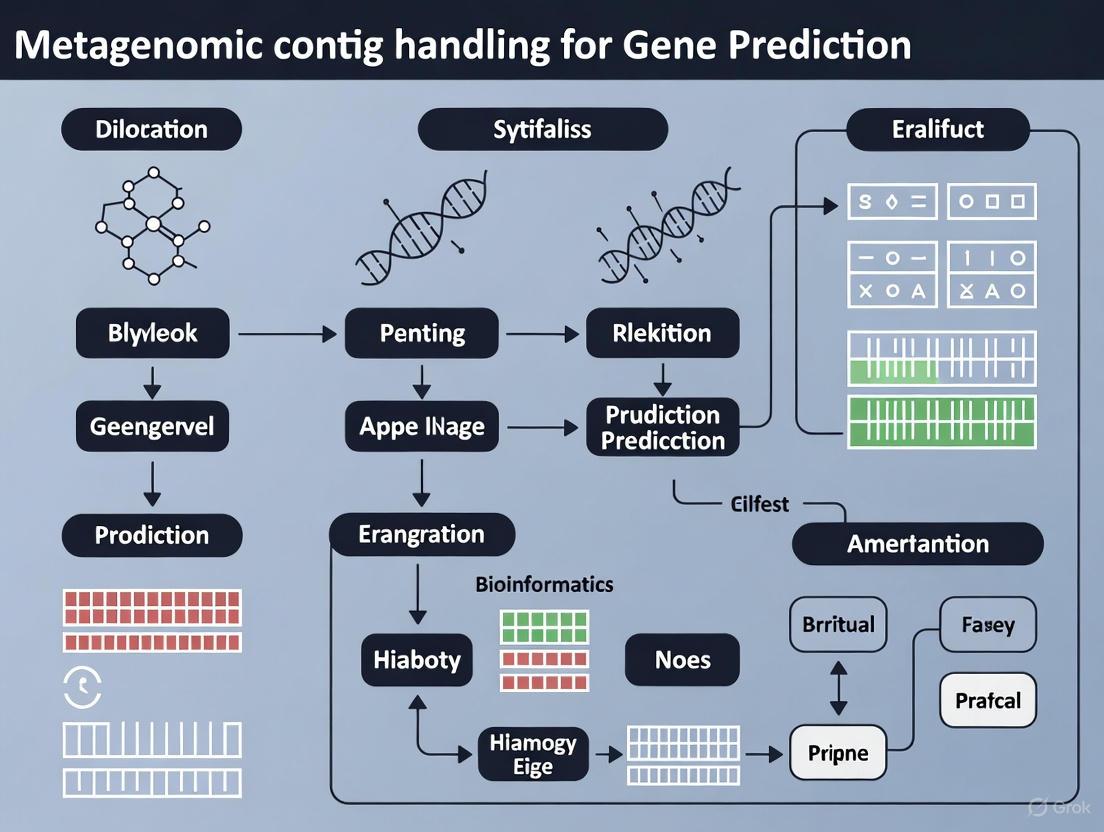
The following workflow diagram illustrates the complete process from sampling to functional analysis:
Workflow for Metagenomic Contig Analysis: This diagram outlines the key stages in processing metagenomic data from environmental samples to biological interpretation, highlighting the central role of contig generation and analysis.
Applications and Protocols
Application Note: Biofuel Enzyme Discovery
Metagenomic contigs have enabled breakthrough applications in industrial biotechnology, particularly in biofuel production. Researchers have discovered numerous lignocellulose-degrading enzymes from uncultured microbes in diverse environments including buffalo rumen, anaerobic digesters, and compost soils [3]. For example, novel thermotolerant cellulases identified from buffalo rumen metagenomes function at elevated temperatures ideal for industrial processes, while halotolerant enzymes from anaerobic beer waste metabolomes remain active in high-salt conditions [3].
These discoveries bypass the traditional limitation of cultivating source organisms, directly addressing the challenge that approximately 99.9% of environmental microbes cannot be cultured using standard methods [3]. The resulting enzymes provide more efficient and cost-effective tools for breaking down plant biomass into fermentable sugars for bioethanol and biodiesel production.
Experimental Protocol: Contig Generation and Analysis
This protocol provides a standardized workflow for generating and analyzing metagenomic contigs from raw sequencing data.
Protocol: Metagenomic Contig Assembly and Gene Prediction
I. Quality Control and Preprocessing
- Quality Assessment: Run FastQC on raw FASTQ files to evaluate per-base sequence quality, GC content, and adapter contamination [8].
- Quality Trimming: Use Trimmomatic or KneadData to remove adapters and trim low-quality bases (Phred score <20). Retain only paired reads after trimming [8].
- Host DNA Removal: Align reads to host reference genome (e.g., GRCh38 for human-associated samples) using Bowtie2 or BWA. Remove aligned reads to enrich for microbial sequences [8].
II. Assembly and Binning
- De Novo Assembly: Run MEGAHIT or metaSPAdes with optimized k-mer ranges. For MEGAHIT, use parameters:
--k-list 27,47,67,87,107,127for progressive k-mer sizes [6] [8]. - Assembly Quality Assessment: Evaluate contig quality using QUAST, reporting N50, largest contig, and total assembly size. Map reads back to contigs with Bowtie2 to estimate assembly completeness [6].
- Binning: Cluster contigs into Metagenome-Assembled Genomes (MAGs) using MetaBAT2 based on coverage and composition. Refine bins with MetaWRAP to achieve >90% completeness and <5% contamination [8].
III. Gene Prediction and Annotation
- Taxonomic Classification: Classify contigs using Kraken2 against standard databases. Apply lineage-specific gene prediction based on taxonomic assignments [10].
- Open Reading Frame Prediction: For bacterial contigs, use Pyrodigal with metagenome mode. For eukaryotic contigs, use AUGUSTUS with appropriate species parameters [10].
- Functional Annotation: Annotate predicted genes using eggNOG-mapper, KofamKOALA for KEGG pathways, and CAZy for carbohydrate-active enzymes [8].
IV. Downstream Analysis
- Gene Abundance Quantification: Map reads to non-redundant gene catalog using Bowtie2. Calculate normalized abundance (TPM) with CoverM [8].
- Statistical Analysis: Identify differentially abundant genes between sample groups using DESeq2 with adjusted p-value < 0.05 [8].
The Scientist's Toolkit: Essential Research Reagents and Computational Tools
Table 4: Essential Resources for Metagenomic Contig Research
| Category | Resource | Specification/Version | Application |
|---|---|---|---|
| Sequencing Kits | Illumina NovaSeq 6000 S4 Reagent Kit | 300-400 Gb output | High-throughput metagenome sequencing |
| DNA Extraction | DNeasy PowerSoil Pro Kit | 100 preps | Inhibitor-free DNA from soil/fecal samples |
| Assembly Software | metaSPAdes | v3.15.5 | High-quality contig assembly |
| Binning Tool | MetaBAT 2 | v2.15 | MAG reconstruction from contigs |
| Gene Predictor | Pyrodigal | v2.0 | Prokaryotic gene finding in metagenomes |
| Taxonomic Classifier | Kraken 2 | v2.1.2 | Rapid taxonomic assignment of contigs |
| Functional Database | eggNOG | v6.0 | Orthology assignments and functional annotation |
| Quality Control | FastQC | v0.12.1 | Quality assessment of sequencing reads |
Metagenomic contigs represent the crucial bridge between raw sequencing data and biologically meaningful insights in cultivation-independent microbial studies. Their generation through sophisticated assembly algorithms and subsequent analysis via lineage-aware annotation pipelines has fundamentally expanded access to the genetic and functional diversity of the microbial world. As protocols standardize and computational methods advance, contig-based approaches will continue to drive discoveries in fields ranging from human health to industrial biotechnology, unlocking the functional potential of Earth's vast uncultured microbial majority.
The workflows and methodologies detailed in this application note provide researchers with robust frameworks for constructing and analyzing metagenomic contigs, emphasizing the importance of appropriate tool selection at each step to maximize biological insight from complex microbial communities.
The accurate reconstruction of genomes from metagenomic sequencing data is a foundational step in microbiome research, enabling the discovery of novel organisms, metabolic pathways, and functional genes. For gene prediction research, the quality of assembled contigs directly impacts the accuracy and completeness of identified gene models. Metagenomic assembly presents unique computational challenges compared to single-genome assembly, primarily due to the presence of multiple organisms at varying abundances, strain-level heterogeneity, shared conserved regions across species, and repetitive genomic elements [11] [6]. Within this context, metaSPAdes and MEGAHIT have emerged as two predominant assemblers, each employing distinct algorithmic approaches to address these challenges. This application note provides a comprehensive comparison of these tools, detailed experimental protocols for their implementation, and their critical connection to downstream gene prediction in metagenomic studies.
metaSPAdes: Advanced Graph-Based Assembly
metaSPAdes is part of the SPAdes toolkit and was specifically designed for large and complex metagenomic datasets. It extends the capabilities of the single-cell SPAdes assembler, which was already adept at handling non-uniform coverage, by incorporating new algorithmic ideas to address metagenomic-specific challenges such as high microdiversity and strain heterogeneity [11]. The assembler operates by first constructing a de Bruijn graph from all reads, then transforming it into an assembly graph using various graph simplification procedures, and finally reconstructing paths in the assembly graph that correspond to long genomic fragments within a metagenome [11]. A key feature of metaSPAdes is its focus on reconstructing a consensus backbone of strain mixtures, which allows it to ignore some strain-specific features corresponding to rare strains, thereby improving assembly contiguity in diverse communities.
MEGAHIT: Efficient Succinct Graph Assembly
MEGAHIT employs a succinct de Bruijn graph (SdBG) approach to achieve highly memory-efficient assembly, making it particularly suitable for large-scale metagenomic projects such as soil microbiomes that require substantial computational resources [12] [6]. It utilizes iterative k-mer sizing with progressively larger values, beginning with smaller k-mers to assemble low-coverage regions and advancing to larger k-mers to resolve repetitive areas [12]. The tool includes several preset parameter configurations optimized for different data types, including "meta" for generic metagenomes, "meta-sensitive" for more comprehensive but slower assembly, and "meta-large" for particularly large and complex metagenomes like soil [12].
Comparative Performance Characteristics
Table 1: Key Characteristics of metaSPAdes and MEGAHIT
| Feature | metaSPAdes | MEGAHIT |
|---|---|---|
| Core Algorithm | de Bruijn graph with graph transformation and path reconstruction [11] | Succinct de Bruijn Graph (SdBG) [12] [6] |
| Memory Usage | Higher memory requirements | Highly memory-efficient [6] |
| Speed | Moderate | Ultra-fast [12] |
| Strengths | Handles strain heterogeneity well; better for complex strain variants [11] [13] | Efficient for large datasets; suitable for low-abundance species [13] [6] |
| Optimal Use Cases | Communities with high microdiversity; strain-resolved analysis [13] | Large-scale metagenomic projects; resource-constrained environments [12] [6] |
Table 2: Performance in Genome Recovery Applications
| Application | metaSPAdes | MEGAHIT | Evidence |
|---|---|---|---|
| Low-Abundance Species Recovery | Highly effective when combined with MetaBAT2 [13] | Moderate performance | Evaluation on human metagenomes [13] |
| Strain-Resolved Genomes | Moderate performance | Excels when combined with MetaBAT2 [13] | Evaluation on real and simulated human metagenomes [13] |
| Assembly of Variable Regions | Good recovery of variable genome regions | Struggles with high-sequence diversity regions [14] | Comparison using paired long-read and short-read data [14] |
Experimental Protocols
Protocol 1: metaSPAdes Assembly Workflow
Principle: metaSPAdes utilizes a multi-stage graph construction and simplification process to resolve complex metagenomic communities, making it particularly effective for samples with significant strain diversity [11].
Procedure:
Input Preparation: Obtain quality-filtered paired-end reads in FASTQ format. Ensure reads have been processed through quality control including adapter removal and trimming.
Basic Assembly Command:
Critical Parameters for Metagenomes:
-k: Specify k-mer sizes manually (e.g.,21,33,55,77,99,121for diverse communities)--meta: Explicit meta-mode for metagenomic assembly-t: Number of threads (adjust based on available computational resources)-m: Memory limit in GB to prevent system overload
Output: The assembly results will be generated in the specified output directory, with
contigs.fastacontaining the final assembled contigs.
Protocol 2: MEGAHIT Assembly Workflow
Principle: MEGAHIT employs iterative k-mer refinement using a memory-efficient succinct de Bruijn graph representation, enabling assembly of large metagenomic datasets on single servers [12] [6].
Procedure:
Input Preparation: Use the same quality-controlled paired-end reads as for metaSPAdes.
Basic Assembly Command:
Critical Parameters and Presets:
--presets: Use preset parameter configurations:meta-sensitive: For more comprehensive assembly (slower)meta-large: For large, complex metagenomes like soil
--min-contig-len: Set minimum contig length output (default: 200)-t: Number of CPU threads-m: Memory usage as fraction of total system memory (default: 0.9)
Output: Assembled contigs are located at
megahit_output/final.contigs.fa.
Protocol 3: Assembly Strategy Selection Framework
Individual vs. Co-assembly Decision Protocol:
Evaluate Sample Characteristics:
- Choose co-assembly when processing samples from the same sampling event, longitudinal sampling of the same site, or related samples with similar community structures [6].
- Choose individual assembly followed by de-replication when working with distinct sampling events, different environments, or communities with substantial strain variation [6].
Co-assembly Advantages and Disadvantages:
Integration with Gene Prediction Research
The connection between assembly quality and gene prediction accuracy cannot be overstated. High-quality assemblies with longer contigs and fewer errors provide more complete gene models with accurate structural annotations. Research has demonstrated that short-read assemblies often struggle with variable regions of genomes, such as integrated viruses or defense system islands, potentially leading to underestimation of true functional diversity [14]. These limitations directly impact downstream gene prediction, as fragmented assemblies may yield partial gene sequences or miss genetically variable elements entirely.
The emergence of hybrid assembly approaches, combining short-read technologies with long-read sequencing from platforms such as Pacific Biosciences (PacBio) or Oxford Nanopore Technologies (ONT), has shown promise in addressing these limitations. Studies comparing long-read and short-read metagenome assemblies indicate that long-read sequencing improves assembly contiguity and recovery of variable regions, thereby providing more complete templates for gene prediction algorithms [14].
For gene prediction on metagenomic assemblies, tools such as Helixer represent advances in ab initio prediction, using deep learning to identify gene structures directly from genomic DNA without requiring additional experimental data such as RNA sequencing [15]. Unlike traditional hidden Markov model-based tools like GeneMark-ES or AUGUSTUS, Helixer operates across fungal, plant, vertebrate, and invertebrate genomes without species-specific training, making it particularly valuable for metagenomic contigs from diverse and uncharacterized organisms [15].
Visualization of Assembly Workflows
metaSPAdes Assembly Workflow
MEGAHIT Assembly Workflow
Table 3: Essential Resources for Metagenomic Assembly and Analysis
| Resource Category | Specific Tools/Components | Function in Workflow |
|---|---|---|
| Primary Assemblers | metaSPAdes, MEGAHIT | Core assembly algorithms for constructing contigs from sequencing reads [11] [12] |
| Quality Assessment | CheckM2, BUSCO, GUNC, QUAST | Evaluate assembly quality, completeness, contamination, and contiguity [16] |
| Gene Prediction | Helixer, GeneMark-ES, AUGUSTUS | Identify and annotate gene structures on assembled contigs [15] |
| Binning Tools | MetaBAT2, SemiBin2 | Group contigs into metagenome-assembled genomes (MAGs) based on sequence composition and coverage [14] [13] |
| Taxonomic Annotation | GTDB-Tk2 | Assign taxonomic classifications to assembled contigs and MAGs [16] |
| Data Sources | NCBI GenBank, IMG/VR | Reference databases for comparative analysis and completeness assessment [17] [15] |
Selection between metaSPAdes and MEGAHIT represents a critical decision point in metagenomic analysis workflows with direct implications for downstream gene prediction research. metaSPAdes excels in environments with significant strain heterogeneity and when assembly quality is prioritized over computational efficiency. In contrast, MEGAHIT offers a robust solution for large-scale metagenomic projects where computational resources are constrained or when processing extremely complex samples such as soil microbiomes. The emerging paradigm of hybrid assembly approaches, leveraging both short and long-read technologies, presents a promising avenue for further improving contiguity and completeness of metagenomic assemblies. As gene prediction algorithms continue to advance, particularly with deep learning approaches like Helixer, the synergy between high-quality assembly and accurate gene annotation will remain fundamental to extracting biological insights from complex microbial communities.
Within the framework of a broader thesis on handling metagenomic contigs for gene prediction research, this application note addresses three critical contig properties—GC-content, the presence of repeat elements, and heterozygosity. These properties significantly influence the quality of metagenome-assembled genomes (MAGs) and the accuracy of subsequent gene prediction and functional annotation [18] [19] [20]. Inaccurate assemblies, driven by these factors, can lead to fragmented genes, false positives in gene calls, and a misrepresentation of the functional potential and antimicrobial resistance (AMR) profiles within a microbial community [19] [21]. This document provides a structured overview of these challenges, summarizes quantitative data, and offers detailed protocols to identify and mitigate their effects, thereby enabling more reliable metagenomic analysis for researchers, scientists, and drug development professionals.
The following tables consolidate key quantitative findings on how GC-content, repeat elements, and heterozygosity impact metagenomic assembly and gene prediction.
Table 1: Impact of GC-Content on Sequencing Coverage and Assembly
| GC Content Range | Observed Coverage Effect | Sequencing Platform | Library Preparation Notes |
|---|---|---|---|
| ~30% GC | >10-fold less coverage vs. 50% GC | Illumina MiSeq/NextSeq | Major bias outside 45-65% GC range [18] |
| 45-65% GC | Optimal (baseline) coverage | Illumina MiSeq/NextSeq | Least biased range for these platforms [18] |
| GC-rich | Falsely low coverage | Illumina MiSeq/NextSeq | Inefficient PCR amplification [18] |
| GC-rich & GC-poor | Under-coverage relative to optimal | Illumina HiSeq, PacBio | Distinct bias profile from MiSeq/NextSeq [18] |
| All ranges | No significant GC bias | Oxford Nanopore | PCR-free workflow [18] |
Table 2: Impact of Repeat Elements and Heterozygosity on Assembly
| Property | Impact on Assembly | Consequence for Gene Prediction |
|---|---|---|
| Antibiotic Resistance Genes (ARGs) | Assemblies tend to break around ARGs [19] | Fragmented ARG contigs lose genomic context and taxonomic origin [19] [21] |
| Mobile Genetic Elements (MGEs) | Highly fragmented, collapsed contigs [21] | Inability to link ARGs to plasmids or phages, misjudging mobilization risk [22] [21] |
| High Heterozygosity (>3%) | Highly fragmented assembly, high duplication rate [20] | Duplicated single-copy genes can be misinterpreted as different genes [20] |
| High Heterozygosity (e.g., 5.29%) | Conventional assembly procedures fail; scaffolds not reaching chromosome level [20] | Hinders accurate biological and genetic research [20] |
Experimental Protocols for Assessing Critical Properties
Protocol: Evaluating and Mitigating GC Bias
1. Objective: To quantify GC-dependent coverage biases in metagenomic sequencing data and account for them in downstream analyses.
2. Materials:
- High-quality metagenomic DNA
- Library preparation kit (note PCR cycles)
- Sequencing platform (e.g., Illumina, Oxford Nanopore)
- Computing resources with bioinformatics software (e.g., FastQC, metaSPAdes, custom scripts)
3. Methodology:
- Library Preparation: If using Illumina, consider PCR-free protocols where possible. If PCR is necessary, optimize polymerase mixtures and use additives like betaine or trimethylammonium chloride to improve coverage of GC-rich and GC-poor regions, respectively [18].
- Sequencing: Select an appropriate sequencing platform. Note that GC bias profiles vary significantly between platforms; Oxford Nanopore has been shown to be largely unaffected by GC bias [18].
- Bioinformatic Analysis:
- Quality Control: Process raw reads with tools like Trimmomatic or PRINSEQ to remove adapters and low-quality bases [23].
- Calculate GC-Coverage Relationship: Map quality-filtered reads to contigs or a reference genome. For each contig (or genomic window), calculate its mean coverage and its GC content.
- Visualization: Create a scatter plot of coverage versus GC content. A neutral profile shows a random scatter, while a biased profile shows a clear curve (e.g., peak at 50% GC) [18].
- Account for Bias: For quantitative metagenomics, use the GC-coverage relationship to correct abundance estimates before drawing ecological conclusions [18].
Protocol: Managing Repetitive Elements and ARGs
1. Objective: To assess the fragmentation of contigs around repetitive elements like ARGs and MGEs and improve their contextual assembly.
2. Materials:
- Metagenomic short-read (Illumina) and/or long-read (Oxford Nanopore, PacBio) data
- High-performance computing infrastructure
- MetaMobilePicker pipeline
- Assembly tools (metaSPAdes, MEGAHIT, Trinity)
- Annotation databases (CARD, mobileOG)
3. Methodology:
- Assembly: Perform de novo assembly using multiple tools. For short reads, metaSPAdes is generally recommended, but for recovering context around repetitive genes, the transcriptome assembler Trinity has shown promise in producing longer, fewer contigs [19].
- Element Identification: Annotate assembled contigs for ARGs using the Comprehensive Antibiotic Resistance Database (CARD) and for MGEs (plasmids, phages, IS elements) using tools integrated in pipelines like MetaMobilePicker [21].
- Fragmentation Assessment:
- Calculate the number of contigs containing ARGs.
- Determine the average length of ARG-containing contigs.
- Check if the ARG is complete and if flanking sequences (e.g., plasmid backbones, chromosomal genes) are present.
- Complementary Quantification: Since assembly often fragments ARGs, directly map quality-filtered reads to an ARG database (e.g., using BWA or Bowtie2) to obtain accurate abundance and diversity measures that are not biased by assembly fragmentation [19].
Protocol: Handling High Heterozygosity in Genomes
1. Objective: To assemble a high-quality genome from a metagenome or isolate with high heterozygosity, minimizing fragmentation and duplication.
2. Materials:
- PacBio long-read data or Hi-C data
- Assemblers: MECAT2, 3d-dna, ALLHiC
- Duplication purging tools: Purgehaplotigs, Purgedups
3. Methodology (Based on the AealbF3 Workflow):
- Read Generation and Draft Assembly: Generate high-coverage long reads (e.g., ~418x PacBio reads). Process and assemble these reads into a draft genome using an assembler like MECAT2 [20].
- Identify Duplication: Use BUSCO to assess single-copy gene duplication. A high duplication rate (>70%) indicates a highly heterozygous assembly [20].
- Extract Flanking Sequences: Identify flanking sequences (>15,000 bp) around duplicated BUSCO genes with the highest BLAST alignment scores [20].
- Chromosome-Level Scaffolding: Map Hi-C data to the extracted flanking sequences. Use the 3d-dna software to generate a Hi-C contact map and cluster sequences into potential chromosomes. Finally, use ALLHiC to orient and order the sequences, producing a chromosome-level assembly [20].
- Evaluation: Assess the new assembly (e.g., AealbF3) for completeness (BUSCO), duplication rate, and contiguity (N50). The goal is a high completeness (>98%) with a low duplication rate (<2%) [20].
The Scientist's Toolkit: Essential Research Reagents and Materials
Table 3: Key Research Reagents and Computational Tools
| Item Name | Function / Application | Specific Example / Note |
|---|---|---|
| Betaine (PCR Additive) | Improves amplification of GC-rich regions during library prep, mitigating coverage bias [18]. | Used in PCR-dependent Illumina library protocols. |
| Oxford Nanopore Tech. | Sequencing platform demonstrating minimal GC bias, advantageous for unbiased coverage [18]. | PCR-free library preparation is a key feature. |
| Trimmomatic | Software for quality filtering of raw sequencing reads; removes adapters and low-quality bases [23]. | Critical pre-processing step before assembly. |
| metaSPAdes | Metagenomic assembler for short reads; generally performs well but may fragment repeats [19] [21]. | Resource-intensive; requires high-performance computing. |
| Trinity | Transcriptome assembler that can be applied to metagenomes to recover longer contigs around conserved genes [19]. | Useful for contextualizing ARGs. |
| Comprehensive Antibiotic Resistance Database (CARD) | Reference database for annotating antibiotic resistance genes in contigs or reads [19]. | Essential for resistome analysis. |
| BUSCO (Benchmarking Universal Single-Copy Orthologs) | Tool to assess genome/completeness and duplication, identifying potentially heterozygous assemblies [20]. | High duplication rate flags heterozygosity. |
| ALLHiC | Software package for scaffolding and ordering contigs into chromosomes using Hi-C data [20]. | Part of the workflow for handling heterozygosity. |
| BWA-MEM / VG | Read alignment tools. VG maps to graph genomes, reducing reference bias and improving accuracy in repetitive regions [24]. | VG is part of a pangenome approach. |
Workflow and Relationship Diagrams
The following diagram illustrates the logical workflow for analyzing a metagenomic sample, highlighting the points at which the three critical contig properties impact the process and the corresponding mitigation strategies.
The assembly of metagenomic samples is paramount for elucidating the mobility potential and taxonomic origin of antibiotic resistance genes (ARGs), information that is critical for assessing public health risks and designing interventions. However, the presence of nearly identical ARGs and other conserved regions across multiple genomic contexts and bacterial species presents a substantial challenge for assembly algorithms [19]. These highly similar sequences create complex, branched assembly graphs that are difficult to resolve, invariably leading to premature contig breaks precisely in the regions of greatest interest [19]. This fragmentation obscures the genomic context of ARGs, including their association with mobile genetic elements (MGEs) and their bacterial host organisms, thereby complicating risk assessment and hindering efforts to track the dissemination of antimicrobial resistance (AMR) [19].
This Application Note delineates the core technical challenges of ARG fragmentation, provides quantitative data from comparative assessments of assembly strategies, and offers detailed protocols for leveraging advanced sequencing and bioinformatic techniques to overcome these hurdles, all within the framework of processing metagenomic contigs for gene prediction research.
Quantitative Assessment of Assembly Performance
Systematic evaluations of assembly tools reveal significant differences in their ability to reconstruct ARGs and their flanking regions. The following tables summarize key performance metrics from controlled benchmarking studies, providing a basis for selecting an appropriate assembly strategy.
Table 1: Performance of Assembly Tools in Recovering ARG Contexts from a Spiked Metagenomic Sample (Short-Read Data) [19]
| Assembly Tool | Assembly Type | Contiguity (Total contig length ≥500 bp) | Ability to Recover Unique Genomic Contexts | Fragmentation Around ARGs |
|---|---|---|---|---|
| metaSPAdes | Metagenomic | Intermediate | Moderate | High |
| MEGAHIT | Metagenomic | Low (very short contigs) | Poor | Very High |
| Trinity | Transcriptomic | High (longer, fewer contigs) | Good | Moderate |
| Velvet | Genomic | Intermediate | Moderate | High |
| SPAdes | Genomic | Intermediate | Moderate | High |
| Ray | Metagenomic | Intermediate | Moderate | High |
Table 2: Benefits of Co-assembly for Improving Assembly Quality in Low-Biomass Airborne Metagenomes [25]
| Assembly Metric | Individual Assembly | Co-assembly | Improvement |
|---|---|---|---|
| Genome Fraction (%) | 4.83 ± 2.71% | 4.94 ± 2.64% | Slight Increase |
| Duplication Ratio | 1.23 ± 0.20 | 1.09 ± 0.06 | Significant Reduction |
| Mismatches per 100 kbp | 4491.1 ± 344.46 | 4379.82 ± 339.23 | Slight Reduction |
| Number of Misassemblies | 410.67 ± 257.66 | 277.67 ± 107.15 | Significant Reduction |
| Total Contig Length (≥500 bp) | 334.31 Mbp | 555.79 Mbp | Substantial Increase |
Detailed Experimental Protocols
Protocol: Long-Read Metagenomic Sequencing for ARG Host Linking
This protocol utilizes Oxford Nanopore Technologies (ONT) long-read sequencing and DNA modification profiling to link plasmids carrying ARGs to their bacterial hosts [26].
I. Sample Preparation and DNA Extraction
- Input: Complex samples (e.g., chicken feces, wastewater, soil).
- Step 1: Preserve samples immediately upon collection using a stabilizer such as DNA/RNA Shield.
- Step 2: Extract high-molecular-weight genomic DNA. Use kits designed for long-read sequencing to maximize DNA integrity and size.
- Quality Control: Verify DNA quantity and quality using a fluorometer and fragment analyzer.
II. Library Preparation and Sequencing
- Step 3: Prepare a sequencing library from native DNA (without PCR amplification) to preserve epigenetic modifications, using ONT's kit (e.g., Ligation Sequencing Kit).
- Step 4: Load the library onto a PromethION flow cell (R10 or newer) and sequence for up to 72 hours using the associated instrument and V14 chemistry.
III. Bioinformatic Analysis for Host Linking
- Step 5: Basecalling and Assembly. Perform high-accuracy basecalling and assemble reads into contigs using a long-read assembler (e.g., Flye).
- Step 6: ARG Identification. Annotate ARGs on contigs using a tool like AMRFinderPlus or by aligning to the Comprehensive Antibiotic Resistance Database (CARD).
- Step 7: Methylation Motif Detection. Use the basecaller to detect DNA modification signals (4mC, 5mC, 6mA) from the raw sequencing data. Subsequently, run a tool like
NanoMotiforMicrobeModto identify active methylation motifs in the assembled contigs. - Step 8: Plasmid-Host Linking. Cluster contigs derived from the same bacterial host by identifying shared, strain-specific methylation motifs. A plasmid contig carrying an ARG will cluster with the chromosomal contigs of its host, enabling confident assignment [26].
Diagram 1: Methylation-based host linking workflow.
Protocol: Co-assembly of Metagenomic Samples for Enhanced ARG Recovery
This protocol is designed for complex, low-biomass samples (e.g., air, water) where individual assembly fails. Co-assembly pools multiple samples to increase effective sequencing depth and improve the recovery of ARG contexts [25].
I. Sample Grouping and Data Pre-processing
- Step 1: Define Subgroups. Group individual metagenomic samples based on shared characteristics, such as sampling time, location, or preliminary taxonomic profile (e.g., via 16S rRNA gene sequencing).
- Step 2: Quality Control and Read Trimming. Process raw sequencing reads for each sample independently using tools like FastQC and Trimmomatic to remove adapters and low-quality bases.
II. Co-assembly Execution
- Step 3: Pool Reads. Concatenate all quality-filtered reads from the samples within a predefined subgroup into a single, large read set.
- Step 4: Perform Co-assembly. Assemble the pooled reads using a metagenome assembler such as metaSPAdes.
metaSPAdes.py --meta -1 pooled_1.fastq -2 pooled_2.fastq -o coassembly_output - Step 5: Assess Assembly Quality. Use tools like Quast or CheckM to evaluate assembly metrics (N50, number of contigs) and compare them against individual assemblies.
III. ARG Annotation and Context Analysis
- Step 6: Identify ARGs. Annotate ARGs on the co-assembled contigs using a database like SARG or CARD.
- Step 7: Quantify Context Improvement. Compare the length of ARG-containing contigs and the presence of flanking MGEs (e.g., using tools like MobileElementFinder) between the co-assembly and individual assemblies.
Protocol: Species-Resolved ARG Profiling with Argo
Argo is a read-based profiler that uses long-read overlapping to accurately assign ARGs to their host species without assembly, thus bypassing fragmentation issues [27].
I. Data Preparation and ARG Screening
- Input: Long reads (ONT or PacBio) from a metagenomic sample.
- Step 1: Identify ARG-Carrying Reads. Align all reads against the SARG+ database (a manually curated expansion of CARD, NDARO, and SARG) using DIAMOND in frameshift-aware mode. This step filters out reads without ARGs.
diamond blastx --db SARGplus --query reads.fastq --out argo_matches.txt --outfmt 6 ...
II. Taxonomic Classification via Read Clustering
- Step 2: Map Reads to Taxonomy Database. Map the ARG-containing reads to a comprehensive taxonomy database (e.g., GTDB) using
minimap2in base-level alignment mode to generate candidate species labels for each read. - Step 3: Build and Segment Overlap Graph. Use
minimap2to compute all-vs-all pairwise overlaps between the ARG-containing reads. Construct an overlap graph and segment it into read clusters using the Markov Cluster (MCL) algorithm. Each cluster ideally represents a single ARG from a specific species. - Step 4: Assign Taxonomy per Cluster. Assign a consensus taxonomic label to all reads within a cluster, rather than to individual reads. This collective assignment significantly enhances accuracy by leveraging the consensus from multiple overlapping sequences [27].
Diagram 2: Argo workflow for species-resolved ARG profiling.
The Scientist's Toolkit: Research Reagent Solutions
Table 3: Essential Resources for Overcoming ARG Fragmentation
| Resource Name | Type | Primary Function | Key Application in Protocol |
|---|---|---|---|
| Oxford Nanopore R10 Flow Cell & V14 Chemistry | Sequencing Hardware | Generates highly accurate long reads with native DNA modification detection. | Enables long-read assembly and methylation-based host linking in Protocol 3.1. |
| SARG+ Database | Bioinformatics Database | A comprehensive, non-redundant ARG protein sequence database. | Used by Argo (Protocol 3.3) for sensitive and specific identification of ARGs from long reads. |
| GTDB (Genome Taxonomy Database) | Bioinformatics Database | A high-quality, standardized microbial taxonomy database. | Provides the reference for accurate taxonomic classification of ARG-containing read clusters in Argo. |
| NanoMotif | Bioinformatics Tool | Detects active DNA methylation motifs from native ONT sequencing data. | Critical for identifying strain-specific signatures to link plasmids to hosts in Protocol 3.1. |
| metaSPAdes | Bioinformatics Tool | A metagenomic assembler designed for complex microbial communities. | The core assembler used for both individual and co-assembly approaches in Protocol 3.2. |
| Trinity | Bioinformatics Tool | A transcriptome assembler repurposed for metagenomics. | Useful for recovering longer contigs around conserved regions in complex samples (Table 1). |
| CRISPR-Cas9 Enrichment | Molecular Biology Method | Enriches low-abundance ARG targets prior to sequencing. | Dramatically lowers detection limits, allowing identification of ARGs missed by standard metagenomics [28]. |
The analysis of microbial communities through metagenomics has revolutionized our understanding of the microbial world, bypassing the need for isolation and lab cultivation of individual species [9]. This approach involves directly sampling and sequencing genetic material from environmental samples, enabling researchers to uncover microbial diversity and functional potential with unprecedented resolution [29]. The fundamental challenge in metagenomics lies in transforming raw sequencing data into accurate, analyzable contigs that faithfully represent the genomic content of complex microbial communities. This process is particularly crucial for downstream applications such as gene prediction, which serves as the gateway to understanding the functional capabilities of microbial ecosystems [9] [30].
The complexity of metagenomic data arises from several factors: the coexistence of thousands of different species in a single sample, highly uneven species abundance, and the fragmented nature of sequencing outputs [9]. For researchers and drug development professionals, establishing a robust, reproducible workflow from raw reads to analyzable contigs is essential for extracting biologically meaningful information that can inform therapeutic discovery and functional characterization. This protocol outlines a comprehensive workflow to address these challenges, incorporating both established practices and recent advancements in the field.
Metagenomic Workflow: From Sample to Contigs
The journey from environmental sample to analyzable contigs involves multiple critical steps, each contributing to the quality and reliability of the final output. The overall workflow, integrating both short-read and long-read approaches, is visualized in Figure 1.
Figure 1. Comprehensive workflow for metagenomic analysis from sample collection to gene prediction. The diagram illustrates the parallel paths for short-read and long-read sequencing technologies, converging at assembly evaluation before proceeding to downstream applications like binning and gene prediction. MAG: Metagenome-Assembled Genome.
Sample Collection and DNA Extraction
The initial steps of sample collection and DNA extraction are critical as they establish the foundation for all subsequent analyses.
Sample Collection: The specific sampling strategy must be tailored to the research question and environment. For instance, rhizosphere studies require collecting soil tightly associated with plant roots, while human gut microbiome investigations necessitate fecal samples [30]. Temporal considerations are also important; in a study of infant viromes, samples were collected at multiple time points following vaccination to capture temporal dynamics [30]. Environmental parameters such as pH, temperature, and nutrient availability should be documented as they help interpret resulting genomic data.
DNA Extraction: This step must efficiently lyse diverse microbial cell types while minimizing bias. A recommended approach uses enzymatic lysis with lysozyme, lysostaphin, and mutanolysin to target different cell wall types, followed by chemical or mechanical disruption [30]. The quality and quantity of extracted DNA should be rigorously assessed using spectrophotometric (e.g., Nanodrop) and fluorometric (e.g., Qubit) methods. For highly complex samples like soil, specialized extraction kits designed for environmental samples often yield better results.
Sequencing Technologies and Library Preparation
Selecting appropriate sequencing technology is crucial and involves trade-offs between read length, accuracy, throughput, and cost.
Table 1: Comparison of Sequencing Technologies for Metagenomics
| Technology | Read Length | Key Advantages | Key Limitations | Ideal Applications |
|---|---|---|---|---|
| Illumina | Short-read (75-300 bp) | High accuracy (<0.1% error rate), high throughput, low cost per base | Short reads complicate assembly in repetitive regions | High-coverage sequencing of low-complexity communities, taxonomic profiling |
| PacBio HiFi | Long-read (10-25 kb) | High accuracy (>99.9%), long reads resolve repeats | Higher DNA input requirements, lower throughput | Complex community assembly, complete genome reconstruction |
| Nanopore | Long-read (up to 2 Mb+) | Real-time sequencing, very long reads, portable options | Higher error rates (5-15%) requiring correction | Complex environmental samples, rapid in-field sequencing |
Library preparation follows standardized protocols specific to each sequencing platform. For Illumina, this typically involves DNA fragmentation, adapter ligation, size selection, and PCR amplification [30]. For long-read technologies, the process often focuses on size selection to maximize read length without fragmentation. Quality control of the final library using bioanalyzer systems or qPCR is essential to ensure sequencing success [30].
Read Processing and Quality Control
Raw sequencing data requires processing to remove low-quality sequences and artifacts before assembly.
Short-Read Processing: Tools like
fastpperform adapter trimming, quality filtering, and read pruning [31]. The default parameters typically include removing bases with quality scores below Q20 and discreads shorter than 50 bp after trimming.Long-Read Processing: Nanopore reads typically require filtering based on quality scores and length. Tools like
NanoFiltremove reads with average quality below Q10 and lengths below 1 kb. For PacBio data, circular consensus sequencing (CCS) mode generates high-fidelity (HiFi) reads by sequencing the same molecule multiple times.
Metagenomic Assembly
Assembly reconstructs contiguous sequences (contigs) from the overlapping reads, which is particularly challenging for metagenomic data due to multiple closely related strains and species.
Table 2: Metagenomic Assemblers and Their Applications
| Assembler | Algorithm Type | Read Type | Key Features | Considerations |
|---|---|---|---|---|
| metaSPAdes [9] | De Bruijn graph | Short-read | Multicut, mismatch correction | Effective for diverse communities but computationally intensive |
| metaFlye [32] [31] | Overlap-layout-consensus | Long-read | --meta flag for metagenomes, repeat resolution |
Good for complex samples, used in the mmlong2 workflow [33] |
| HiCanu [32] | Overlap-layout-consensus | Long-read | Adapted from Canu for HiFi data, high accuracy | Resource-intensive, requires high-memory computing |
| hifiasm-meta [32] | Graph-based | Long-read | Optimized for PacBio HiFi data, haplotype resolution | Fast assembly with good contiguity |
| metaMDBG [32] | Graph-based | Long-read | Minimizer-based, memory efficient | Suitable for large datasets, multiple versions available |
Recent advancements in long-read sequencing have dramatically improved metagenomic assembly. The mmlong2 workflow exemplifies this progress, incorporating multiple optimizations for recovering prokaryotic genomes from complex samples, including differential coverage binning, ensemble binning (using multiple binners), and iterative binning [33]. This approach recovered over 15,000 previously undescribed microbial species from terrestrial samples, expanding the phylogenetic diversity of the prokaryotic tree of life by 8% [33].
Assembly Quality Assessment and Contig Binning
Evaluating assembly quality is crucial before proceeding to downstream analyses. Key metrics include contiguity (N50, L50), completeness, and contamination. CheckM2 is widely used for assessing completeness and contamination of metagenome-assembled genomes (MAGs) [34]. For a more thorough evaluation, anvi-script-find-misassemblies can identify potential assembly errors by examining long-read mapping patterns [32].
Contig binning groups assembled contigs into MAGs representing individual populations. This can be achieved through composition-based methods (using k-mer frequencies) and/or abundance-based methods (using coverage patterns across multiple samples). The mmlong2 workflow demonstrates the power of combining multiple binning strategies to maximize MAG recovery from complex samples [33].
The Scientist's Toolkit: Essential Research Reagents and Computational Tools
Successful metagenomic analysis requires both wet-lab reagents and computational tools. The following table summarizes key components of the metagenomics toolkit.
Table 3: Essential Research Reagent Solutions and Computational Tools for Metagenomic Analysis
| Category | Item/Software | Specific Application/Function | Key Features/Benefits |
|---|---|---|---|
| Wet-Lab Reagents | Lysozyme, Lysostaphin, Mutanolysin | Enzymatic cell lysis in DNA extraction | Targets diverse cell wall types; increases DNA yield from complex samples |
| PACBIO SMRTbell Express Template Prep Kit | Library preparation for PacBio sequencing | Optimized for long-read sequencing; maintains DNA integrity | |
| Illumina DNA Prep Kits | Library preparation for Illumina sequencing | High-efficiency adapter ligation; compatible with low-input samples | |
| Computational Tools | fastp [31] |
Quality control and adapter trimming | Fast processing; integrated quality reporting |
metaFlye [32] |
Long-read metagenomic assembly | Resolves repetitive regions; --meta flag for complex communities |
|
CheckM2 [34] |
Assembly quality assessment | Estimates completeness and contamination; rapid analysis | |
CompareM2 [34] |
Comparative genome analysis | Easy installation; comprehensive reporting for bacterial/archaeal genomes | |
AMRomics [31] |
Large-scale microbial genome analysis | Scalable to thousands of genomes; supports progressive analysis | |
Meteor2 [35] |
Taxonomic, functional, and strain-level profiling | Uses environment-specific gene catalogs; improved sensitivity for low-abundance species | |
Prokka [31] |
Genome annotation | Rapid annotation; standardized output format | |
Bakta [34] |
Genome annotation | Comprehensive functional annotation; database included |
Downstream Analysis: Connecting Contigs to Gene Prediction
The ultimate goal of generating analyzable contigs is to enable biological insights through downstream analyses such as gene prediction and functional annotation.
Gene Prediction Approaches
Gene prediction in metagenomic data presents unique challenges compared to isolate genomes, including fragmented genes and unknown source organisms [9]. Three primary approaches have been developed:
Homology-based methods (e.g., CRITICA, Orpheus) use BLAST against known protein databases but cannot predict novel genes without homologs [9].
Model-based methods (e.g., MetaGeneMark, FragGeneScan) employ hidden Markov models or higher-order Markov chains but require thousands of parameters [9].
Machine learning-based methods (e.g., MetaGUN, Orphelia) use features like codon usage, open reading frame (ORF) length, and sequence patterns to train classifiers for gene identification [9].
The Meta-MFDL predictor represents a recent advancement, fusing multiple features (monocodon usage, monoamino acid usage, ORF length coverage, and Z-curve features) with deep stacking networks to improve prediction accuracy [9]. For ORFs shorter than 60 bp, which are typically too short to provide useful information, prediction is generally not recommended [9].
Functional Annotation and Interpretation
After gene prediction, functional annotation assigns biological meaning to predicted genes. This typically involves comparing protein sequences against databases such as KEGG for metabolic pathways, dbCAN for carbohydrate-active enzymes, and AMRFinderPlus for antimicrobial resistance genes [34] [35] [31]. Tools like CompareM2 and AMRomics integrate multiple annotation sources to provide comprehensive functional profiles [34] [31].
Advanced approaches are emerging that leverage machine learning to extract deeper insights from genomic context. The genomic language model (gLM) trains transformer neural networks on millions of metagenomic scaffolds to learn functional and regulatory relationships between genes, demonstrating that contextualized protein embeddings can capture biologically meaningful information such as enzymatic function and taxonomic affiliation [36].
The workflow from raw reads to analyzable contigs represents the foundational pipeline in metagenomic studies, determining the quality and reliability of all subsequent biological interpretations. As sequencing technologies continue to evolve, with long-read approaches enabling more complete genome reconstruction from complex samples [33], and computational methods advance through deep learning approaches [9] [36], this workflow continues to improve in both accuracy and accessibility.
For researchers focused on gene prediction from microbial communities, establishing a robust and reproducible workflow following the protocols outlined in this application note is essential. The integration of wet-lab protocols with computational tools, coupled with rigorous quality control at each step, ensures that resulting contigs faithfully represent the microbial community under investigation. This foundation enables accurate gene prediction and functional annotation, ultimately supporting drug discovery and broader microbial ecology research.
Gene Prediction Methodologies: From Ab Initio Tools to Deep Learning Applications
Within the framework of metagenomic contig analysis, ab initio gene prediction represents a critical first step in deciphering the functional potential of uncultured microorganisms. This methodology identifies protein-coding genes directly from nucleotide sequences by leveraging intrinsic signals—such as codon usage, ribosome binding sites, and GC frame bias—without relying on experimental data or homology comparisons [37] [38]. In metagenomics, where a substantial proportion of sequences originate from unknown and uncharacterized organisms, this reference-independent approach is indispensable for discovering novel genes and functions [39].
The computational challenge is substantial. Metagenomic assemblies present fragmented sequences from diverse organisms with varying genomic signatures, complicating the accurate delineation of gene boundaries [40] [41]. This application note details standardized protocols for employing two preeminent ab initio prediction tools, Prodigal and MetaGeneMark, within metagenomic research workflows. We provide experimental validations and performance benchmarks to guide researchers in their effective application.
Prodigal (PROkaryotic DYnamic programming Gene-finding ALgorithm)
Prodigal employs a dynamic programming algorithm to identify the optimal tiling path of genes across a genomic sequence [37]. Its strength lies in its unsupervised operation; it automatically derives a training profile from the input sequence, capturing characteristics like start codon usage, ribosomal binding site motifs, and GC content bias. A key feature is its use of the GC frame plot, which analyzes the bias for guanine and cytosine in the three codon positions across a 120-base pair window to distinguish coding from non-coding regions [37].
MetaGeneMark
The MetaGeneMark algorithm utilizes inhomogeneous Markov models of orders 3, 4, and 5 to model protein-coding regions [42]. The MetaGeneMark software is often applied with models pre-computed for sequences with specific GC content. For more advanced analysis, the GeneMark-HM pipeline leverages a database of pan-genomes from human microbiome species. It assigns a nearly optimal model to each metagenomic contig by first performing a similarity search of initially predicted genes against the pan-genome database. If a close relative is found, the corresponding species-specific model is used for a more accurate prediction; otherwise, the contig is analyzed by the self-training GeneMarkS-2 or the standard MetaGeneMark with GC-specific models [42].
The Scientist's Toolkit: Essential Research Reagents
The following table catalogues the key computational tools and databases essential for implementing the ab initio gene prediction protocols described in this note.
Table 1: Key Research Reagent Solutions for Ab Initio Gene Prediction
| Name | Type | Primary Function |
|---|---|---|
| Prodigal [37] | Gene Prediction Algorithm | Accurately predicts prokaryotic genes and translation initiation sites in isolated genomes and metagenomic contigs. |
| MetaGeneMark [42] | Gene Prediction Algorithm | Predicts genes in metagenomic fragments using Markov models and GC content-specific models. |
| GeneMark-HM [42] | Metagenomic Annotation Pipeline | Improves prediction accuracy in human microbiome samples using a pan-genome database for model selection. |
| geneRFinder [38] | Machine Learning Gene Finder | Identifies coding sequences and intergenic regions using a Random Forest model, designed for complex metagenomes. |
| FragGeneScan [40] | Gene Prediction Algorithm | A tool designed for predicting genes in fragmented metagenomic data, accounting for sequencing errors. |
| CheckM [43] | Genome Quality Assessment Tool | Evaluates the completeness and contamination of Metagenome-Assembled Genomes (MAGs) post-binning. |
| KEGG [44] | Functional Database | Used for the functional annotation of predicted genes, particularly for mapping onto metabolic pathways. |
| eggNOG [44] | Functional Database | Provides orthologous group information for functional annotation and evolutionary analysis of predicted genes. |
| GTDB-tk [40] | Taxonomic Classification Tool | Assigns taxonomic labels to MAGs based on the Genome Taxonomy Database. |
Experimental Protocols & Performance Benchmarks
Protocol: Gene Prediction with Prodigal on Metagenomic Contigs
This protocol is designed for predicting open reading frames (ORFs) from a set of assembled metagenomic contigs.
- Input Preparation: Ensure your input is a FASTA file containing assembled metagenomic contigs. Contigs are typically generated from short-read (e.g., Illumina) or long-read (e.g., PacBio) assemblers like metaSPAdes or Flye [40] [41].
- Tool Execution: Run Prodigal in "metagenomic" mode, which uses a pre-trained model suitable for mixed communities.
-i: Input contig FASTA file.-o: Output gene models in GFF format.-a: Output predicted protein sequences in FASTA format.-d: Output predicted nucleotide coding sequences (CDS) in FASTA format.-p meta: Selects the metagenomic mode.
- Output Interpretation: The GFF file contains the precise coordinates, strand, and frame for each predicted gene. The protein and CDS FASTA files are used for downstream functional annotation (e.g., with KEGG or eggNOG via DIAMOND/BLAST+) [44].
Protocol: Gene Prediction with MetaGeneMark
- Input Preparation: Prepare your metagenomic contigs in a FASTA file.
- Tool Execution: Run MetaGeneMark. The following command uses a model file for general metagenomic data.
-M: Specifies the model file (e.g., for metagenomes).-f G: Output in GFF format.-oand-d: Define output files for coordinates and CDS sequences.
- Output Interpretation: Similar to Prodigal, the outputs are coordinate and sequence files for downstream analysis.
Performance Benchmarking
Independent evaluations provide critical insights into tool performance. A 2021 study introduced geneRFinder and benchmarked it against other tools on datasets of varying complexity [38]. The results demonstrated that tool performance is context-dependent.
Table 2: Gene Prediction Tool Performance on Isolated Genomes and Metagenomic Data [38]
| Tool | Reported Sensitivity on Genomes | Reported Specificity on Genomes | Reported Sensitivity on High-Complexity Metagenome | Reported Specificity on High-Complexity Metagenome |
|---|---|---|---|---|
| geneRFinder | 95.8% | 95.7% | 89.5% | 90.1% |
| Prodigal | 94.3% | 93.9% | 58.1% | 84.3% |
| FragGeneScan | 89.9% | 89.7% | 34.9% | 11.2% |
A separate 2021 analysis (ORForise) of 15 CDS predictors concluded that no single tool ranked as the most accurate across all tested genomes or metrics, emphasizing that performance is highly dependent on the genome being analyzed [39]. This underscores the value of a multi-tool approach for comprehensive annotation.
Impact of Sequencing Technology on Prediction
The choice of sequencing technology influences assembly continuity, which in turn affects gene prediction. A 2023 study comparing short-read (Illumina) and long-read (PacBio) metagenomics found that while short-read data recovered a greater number of MAGs due to higher sequencing depth, long-read data produced MAGs of higher quality [40]. Specifically, 88% of long-read MAGs included a 16S rRNA gene, compared to only 23% of short-read MAGs [40]. This superior contiguity of long-read assemblies provides more complete genomic context, facilitating more accurate and complete gene prediction.
Integrated Analysis Workflow
The gene prediction process is one component of a larger genome-resolved metagenomics workflow [41]. The diagram below illustrates the logical sequence of steps from raw sequencing data to functional and taxonomic insights, highlighting the role of ab initio prediction.
Figure 1: Genome-resolved metagenomic analysis workflow. Ab initio gene prediction is a pivotal step that connects assembled genomes to functional interpretation. MAGs are generated by binning contigs based on sequence composition and coverage [41] [43].
Technical Notes & Best Practices
- Tool Selection: For standard prokaryotic genomes and simple metagenomes, Prodigal is highly efficient and accurate [37]. For complex human microbiome samples, the GeneMark-HM pipeline, which integrates MetaGeneMark with a pan-genome database, may offer improved accuracy [42]. In cases of high metagenomic complexity, machine learning-based tools like geneRFinder can potentially outperform traditional methods [38].
- Start Codon Accuracy: Prodigal was explicitly designed to improve the identification of translation initiation sites (TIS), a known weakness in earlier algorithms. Its dynamic programming approach, trained on manually curated genomes, allows it to outperform tools that require a separate start-codon refinement step [37].
- Addressing Tool Bias: Be aware that gene prediction tools, especially those trained on model organisms, can exhibit biases that cause them to miss genes with atypical features (e.g., non-standard codon usage, short length, or overlapping genes) [39]. This can hinder the discovery of novel genomic elements.
- Quality Control: Always assess the quality of your input MAGs using tools like CheckM before performing gene prediction [43]. High contamination levels can lead to erroneous gene calls.
Within the broader scope of metagenomic contig analysis, homology-based gene prediction serves as a fundamental methodology for annotating putative genes and inferring their biological functions. Unlike ab initio methods that rely solely on statistical models of coding sequences, homology-based approaches leverage vast repositories of known proteins to identify evolutionarily related sequences through sequence similarity searching [45] [46]. The Basic Local Alignment Search Tool (BLAST) algorithm, particularly the BLASTp program for protein-protein comparisons, represents the gold standard for this purpose [47] [48]. This protocol details the application of BLAST-based methods for identifying known genes within metagenomic contigs, a critical step in functional metagenomics that enables researchers to decipher the metabolic potential and ecological roles of uncultured microbial communities [49] [10].
The strategic importance of homology-based annotation is particularly evident in metagenomic studies, where a significant proportion of sequenced data originates from previously uncharacterized organisms [49]. For instance, recent analyses of human gut viromes revealed that approximately 72% (788 out of 1,090) of high-quality viral genomes showed no significant similarity to sequences in the NCBI viral RefSeq database, underscoring both the vast unexplored genetic diversity and the critical need for sensitive annotation methods [49]. Furthermore, in metaproteomic studies, the accuracy of taxonomic annotation directly impacts the quality of downstream functional analyses, with optimized pipelines like ConDiGA (Contigs Directed Gene Annotation) demonstrating that refined BLAST-based searches against carefully selected reference species significantly improve protein identification rates compared to uncurated database searches [50].
Principles of Homology-Based Gene Prediction
Fundamental Concepts
Homology-based gene prediction operates on the principle that evolutionarily related proteins share detectable sequence similarity despite accruing mutations over time. The core assumption is that sequence similarity implies functional relatedness and common evolutionary ancestry. In metagenomic analysis, this approach is particularly valuable because it can provide functional insights for genes from poorly characterized taxa that lack appropriate training data for ab initio prediction tools [10].
The BLAST algorithm implements a heuristic approach to identify High-scoring Segment Pairs (HSPs) between a query sequence and subjects in a database. For protein BLAST (BLASTp), the comparison assesses the similarity between amino acid sequences using substitution matrices (e.g., BLOSUM62) which assign scores to amino acid substitutions based on their observed frequencies in known protein families [48] [51]. The statistical significance of each match is expressed as an E-value, which represents the number of alignments with equivalent scores expected to occur by chance in a database of a given size. Lower E-values indicate more significant matches, with typical thresholds for homology set at 1e-5 or lower [52].
Integration with Metagenomic Analysis Workflows
In comprehensive metagenomic studies, homology-based methods typically follow contig assembly and often complement ab initio gene prediction. As illustrated in Figure 1, the process begins with quality-filtered metagenomic contigs that undergo initial gene calling, after which the predicted protein sequences are searched against reference databases. Recent advances emphasize the importance of lineage-specific approaches, where taxonomic assignment of contigs informs subsequent database selection and search parameters [10]. This strategy has been shown to increase the landscape of captured microbial proteins by 78.9% compared to non-specific approaches [10].
Figure 1. Workflow for homology-based gene annotation in metagenomic analysis. The process begins with assembled contigs, proceeds through gene prediction and translation to protein sequences, followed by BLASTp analysis against reference databases, and culminates in functional annotation based on significant homologs.
Materials and Equipment
Research Reagent Solutions
Table 1: Essential computational tools and databases for homology-based gene prediction
| Tool/Database | Type | Primary Function | Application Notes |
|---|---|---|---|
| BLAST+ Suite [47] [48] | Software Package | Command-line tools for sequence similarity searching | Includes blastp for protein-protein comparisons; essential for high-throughput analysis |
| NCBI nr Database | Protein Database | Comprehensive non-redundant protein sequence collection | General-purpose database; may require filtering for specific taxonomic groups |
| UniProtKB/TrEMBL | Protein Database | Automatically annotated and non-reviewed protein sequences | Larger but less curated than Swiss-Prot; useful for discovering novel homologs [53] |
| Meta4 | Web Application | Sharing and annotating metagenomic gene predictions | Provides dynamic interface with web services for up-to-date BLAST annotations [53] |
| Kaiju | Taxonomy Analysis Tool | Taxonomic classification of metagenomic sequences | Protein-level classification; useful for contig-directed annotation strategies [50] |
| Prodigal | Gene Predictor | Prokaryotic gene prediction in metagenomes | Often used prior to BLAST analysis to generate protein queries from contigs [45] |
Computational Requirements
The computational resources required for homology-based analysis vary significantly based on dataset size and database selection. For typical metagenomic studies containing thousands of contigs, a multi-core server with substantial RAM (≥64 GB) is recommended. BLASTp searches against comprehensive databases like NCBI nr can be computationally intensive, with search time proportional to both query and database sizes. For large-scale projects, consider distributed computing approaches or optimized BLAST implementations such as DIAMOND for accelerated processing.
Experimental Protocol
Preliminary Gene Prediction
Before performing homology searches, protein-coding regions must be identified on metagenomic contigs:
- Contig Preparation: Ensure contigs are in FASTA format. Quality filter based on length and coverage thresholds appropriate to your study.
- Gene Calling: Apply prokaryotic gene prediction tools to identify open reading frames (ORFs). For metagenomic data, recommended tools include:
- Protein Translation: Extract predicted protein sequences in FASTA format. Maintain careful tracking of nucleotide-to-protein correspondence for downstream validation.
BLASTp Database Selection and Preparation
Database selection critically impacts annotation accuracy and computational efficiency:
Database Options:
- Full comprehensive databases (e.g., NCBI nr, UniProtKB) offer broad coverage but increased search time and potential for ambiguous matches
- Taxonomically restricted databases focused on expected clades improve specificity and speed [50]
- Custom databases compiled from specific reference genomes provide highest precision for targeted studies
Database Download and Configuration:
BLASTp Execution and Parameter Optimization
Execute BLASTp searches with parameters optimized for metagenomic data:
Basic Command Structure:
Critical Parameter Settings:
- E-value threshold: Set between 1e-3 and 1e-5 based on desired stringency [52]
- Output format: Use tabular format (outfmt 6) with specific columns for downstream processing
- Coverage filters: Implement query coverage thresholds (qcovs) to avoid partial matches
Advanced Filtering: For homology inference, apply post-processing filters:
- Minimum percent identity (typically 30-90% depending on evolutionary distance)
- Minimum query coverage (≥70% recommended to avoid domain-only matches)
- Bitscore thresholds relative to database size
Table 2: Key BLASTp output fields and their interpretation for homology assessment
| Output Field | Description | Interpretation Guidelines |
|---|---|---|
| pident | Percentage identity | >90% suggests recent common ancestry; 30-50% may indicate distant homology |
| evalue | Expect value | Lower values indicate greater significance; <0.00001 recommended for homologs |
| qcovs | Query coverage | Percentage of query sequence covered by all HSPs; high values (>80%) indicate full-length matches |
| qcovhsp | HSP coverage | Coverage by single High-scoring Segment Pair; reveals potential multi-domain structure |
| bitscore | Normalized score | Alignment quality independent of database size; useful for comparing matches across databases |
Results Interpretation and Homology Assessment
Proper interpretation of BLAST results requires integrating multiple metrics:
- Multi-HSP Analysis: Examine the arrangement of High-scoring Segment Pairs. Multiple disjoint HSPs may indicate multi-domain proteins or gene fusion/fission events [52].
- Taxonomic Consistency: Assess whether top hits originate from phylogenetically coherent groups, which increases confidence in homology calls.
- Consensus Annotation: Transfer functional annotations from the best significant hits, giving preference to experimentally characterized proteins in well-studied model organisms.
Applications and Case Studies
Novel Viral Genome Characterization
In a recent study profiling human gut viromes, homology-based methods were instrumental in characterizing 1,090 high-quality viral genomes. After initial gene prediction, BLASTp analysis revealed seven core genes (antB, dnaB, DNMT1, DUT, xlyAB, xtmB, and xtmA) associated with metabolism and fundamental viral processes. Additionally, homology searches identified genes for virulence, host-takeover, drug resistance, tRNA, tmRNA, and CRISPR elements, providing functional insights into previously uncharacterized viral diversity [49].
Enhanced Metaproteomic Analysis
The ConDiGA (Contigs Directed Gene Annotation) pipeline demonstrated that refined homology-based annotation significantly improves metaproteomic analyses. By first annotating contigs and then performing gene-level BLAST searches against the most confident species, this approach increased both the accuracy and yield of protein identifications compared to direct gene annotation against comprehensive databases. In benchmark testing with a synthetic microbial community of 12 species, the ConDiGA pipeline with BLAST-based annotation correctly identified nearly all expected species with minimal false positives [50].
Lineage-Specific Protein Catalog Expansion
A lineage-specific microbial protein prediction approach applied to 9,634 human gut metagenomes leveraged homology-based methods to expand the known protein repertoire of the gut microbiome. By using taxonomic assignment to guide database selection and search parameters, this method increased the landscape of captured microbial proteins by 78.9% compared to standard approaches. The resulting MiProGut catalogue contained 29,232,510 protein clusters, dramatically expanding the reference resource available for homology searches in future studies [10].
Troubleshooting and Optimization
Common Challenges and Solutions
Table 3: Troubleshooting guide for homology-based gene prediction
| Problem | Potential Causes | Solutions |
|---|---|---|
| Low annotation rate | Novel sequences with distant homologs | Use profile-based methods (HMMER) after BLAST; relax E-value threshold with additional validation |
| Over-annotation of common domains | Ubiquitous protein domains triggering false positives | Implement query coverage filters; examine domain architecture using InterProScan [53] |
| Taxonomically inconsistent hits | Horizontal gene transfer; database contamination | Apply taxonomic consistency filters; verify with contig taxonomy from complementary tools like Kaiju [49] |
| Partial gene matches | Fragmented assemblies; gene boundaries | Use qcovs filters (>70%); integrate with ab initio predictions to verify gene structures [52] |
Advanced Optimization Strategies
Iterative Search Approaches: For poorly characterized gene families, perform initial searches with relaxed thresholds, build multiple sequence alignments from significant hits, and use these to search again with more sensitive profile-based methods.
Meta4 Web Services Integration: Implement dynamic annotation systems that use web services to provide up-to-date BLAST results against current databases, overcoming the limitation of static annotations in rapidly growing sequence databases [53].
Complementary Tool Integration: Combine BLAST results with outputs from complementary annotation pipelines:
Figure 2. Multi-factor validation approach for BLAST results. Significant hits should be evaluated through taxonomic consistency filters, coverage analysis, and domain assessment before making functional inferences.
Homology-based methods using BLAST against protein databases remain an indispensable component of metagenomic gene prediction research. When properly implemented with appropriate database selection, parameter optimization, and results validation, these approaches provide reliable functional annotations that form the foundation for downstream ecological and functional interpretations. The integration of BLAST-based methods with complementary tools and lineage-specific strategies significantly enhances annotation accuracy, enabling researchers to extract meaningful biological insights from complex metagenomic datasets.
As sequence databases continue to expand and protein family representations improve, the power of homology-based approaches will further increase. However, researchers should remain mindful of the limitations of these methods, particularly for highly divergent sequences from novel taxonomic groups, and employ complementary approaches when exploring the frontiers of microbial diversity.
Comparative gene prediction represents a significant advancement in bioinformatics by leveraging evolutionary conservation patterns to identify genes and functional elements in genomic sequences. This approach operates on the fundamental principle that functional genomic elements, such as coding regions, tend to be conserved across related species due to selective pressure, while non-functional sequences diverge more rapidly through neutral evolution [54]. The accuracy of gene prediction increases substantially when incorporating comparative genomic information, as conservation provides a powerful filter against false-positive predictions that plague single-genome approaches.
TWINSCAN stands as a pioneering algorithm in this domain, specifically designed to exploit conservation signatures from evolutionarily related "informant" genomes to improve gene structure prediction in a target genome [55]. Unlike earlier ab initio methods like GENSCAN that relied solely on statistical patterns within a single genome, TWINSCAN simultaneously maximizes the probability of gene structures in the target genome and the evolutionary conservation derived from informant genomic sequences [56]. This dual approach dramatically reduces false-positive predictions while maintaining high sensitivity, representing a crucial milestone in the evolution of computational gene finding methods [55].
In the context of metagenomic research, where assembled contigs often originate from previously uncharacterized organisms, comparative gene prediction takes on heightened importance. Traditional ab initio methods struggle with metagenomic data due to the lack of appropriate training sets and the fragmentary nature of assemblies. By utilizing conservation patterns, even in the absence of closely related reference genomes, tools like TWINSCAN provide a robust framework for initial gene annotation of metagenomic contigs, laying essential groundwork for downstream functional analysis and taxonomic classification.
Theoretical Foundation: Computational Principles of TWINSCAN
Algorithmic Architecture and Conservation Integration
TWINSCAN employs a generalized hidden Markov model (GHMM) framework that incorporates evolutionary conservation directly into the gene prediction process. The algorithm builds upon the GENSCAN architecture but extends it by integrating alignment information between the target genome and one or more informant genomes [55]. The model defines states corresponding to gene components (exons, introns, intergenic regions) and transitions between these states, with emission probabilities that account for both sequence composition and conservation patterns.
A key innovation in TWINSCAN is its treatment of conservation as an additional observable signal alongside the DNA sequence itself. The algorithm uses a "conservation sequence" derived from pairwise alignments between the target and informant genomes. This conservation sequence is represented symbolically, with different values indicating the quality and type of alignment at each position [56]. During the gene prediction process, TWINSCAN evaluates both the intrinsic genomic signals (splice sites, start/stop codons, coding potential) and the extrinsic conservation evidence to determine the most probable gene structure.
The statistical framework of TWINSCAN calculates the joint probability of the observed target sequence and conservation sequence given a potential gene structure. This approach allows the model to penalize gene predictions that exhibit poor conservation in putatively coding regions while favoring predictions where exonic regions show higher conservation than adjacent non-coding sequences. The parameters governing these conservation expectations are learned from training sets of known genes, making the algorithm adaptable to different evolutionary distances and taxonomic groups.
Evolutionary Models and Parameterization
TWINSCAN's performance is highly dependent on appropriate parameter files that capture the specific evolutionary relationship between the target and informant species. These parameter files are sensitive to evolutionary distance, as different conservation levels are expected for closely versus distantly related species [56]. The algorithm includes specialized parameter sets for various taxonomic groups, including mammals, Caenorhabditis, Dicot plants, and Cryptococci, each optimized for the appropriate evolutionary context.
The conservation model in TWINSCAN accounts for several evolutionary phenomena: (1) the higher conservation of coding sequences versus non-coding regions, (2) the conservation of reading frame in coding regions, (3) the specific conservation patterns around splice sites, and (4) the different evolutionary rates at first, second, and third codon positions. By modeling these phenomena explicitly, TWINSCAN can distinguish between genuine coding sequences and conserved non-coding elements that might otherwise mislead simpler conservation-based methods.
Table: TWINSCAN Parameter Files for Different Taxonomic Groups
| Target Organism | Informant Organism | Parameter File Features | Intron Length Model |
|---|---|---|---|
| H. sapiens (Human) | M. musculus (Mouse) | Generic mammalian parameters; EST mode available | Standard model |
| C. elegans | C. briggsae | Explicit intron length model up to 4000 bases | Extended model |
| A. thaliana | B. oleracea | Dicot plant-specific parameters | Up to 2000 bases |
| Cryptococcus | Species-specific | Fungal-specific parameters | Standard model |
TWINSCAN Protocol for Metagenomic Contig Annotation
Input Preparation and Data Requirements
The successful application of TWINSCAN to metagenomic contigs requires careful preparation of input data. The protocol begins with the assembly of metagenomic sequencing reads into contigs, followed by several preprocessing steps to optimize prediction accuracy.
Step 1: Contig Quality Assessment and Selection
- Filter metagenomic assemblies to retain contigs >500 bp in length, as shorter sequences provide insufficient context for reliable gene prediction [56]
- Assess contig quality using metrics such as N50, coverage depth, and assembly completeness
- Retain contigs with minimal misassembly indicators as flagged by tools like CheckV [49]
Step 2: Repeat Masking
- Identify and mask repetitive elements using RepeatMasker with MaskerAid improvements [56]
- Repeat masking is critical for reducing false-positive predictions, as repetitive regions can mimic gene-like signals
- For metagenomic data, consider using custom repeat libraries derived from related cultured organisms if available
Step 3: Informant Genome Selection and Database Construction
- Identify appropriate informant genomes based on taxonomic proximity to the expected organisms in the metagenomic sample
- For diverse metagenomic samples with unknown composition, use multiple informant genomes spanning different taxonomic groups
- Construct BLAST databases from the informant genomes for subsequent alignment steps [56]
Step 4: Generation of Conservation Sequences
- Align target contigs against informant databases using WU-BLAST or NCBI BLAST with appropriate parameters [56]
- Convert BLAST outputs to conservation sequences using the
conseq.plscript provided in the TWINSCAN distribution - The conservation sequence format consists of a definition line with BLAST database name followed by a line of conservation symbols (numerical values) [56]
Table: Bioinformatics Tools for TWINSCAN Input Preparation
| Tool | Function | Key Parameters | Application Context |
|---|---|---|---|
| RepeatMasker | Identifies and masks repetitive elements | -species option for taxonomic specificity | Essential for reducing false positives |
| WU-BLAST/NCBI BLAST | Generates alignments between target and informant | E-value cutoff, scoring matrix, gap penalties | Must be optimized for evolutionary distance |
| conseq.pl | Converts BLAST output to conservation sequence | Default parameters typically sufficient | TWINSCAN-specific script |
| CheckV | Assesses contig quality and completeness | --database flag for viral contigs | Particularly valuable for virome studies [49] |
TWINSCAN Execution and Output Interpretation
Step 1: Parameter File Selection
- Select the appropriate parameter file based on the taxonomic context of the analysis
- For metagenomic samples with uncertain taxonomy, begin with general eukaryotic parameters and iterate with more specific parameters as taxonomic affiliations become clearer
- Parameter files are available for mammals, Caenorhabditis, Dicot plants, and Cryptococci in the standard TWINSCAN distribution [56]
Step 2: Running TWINSCAN
- Execute TWINSCAN using the command:
twinscan [parameters] [target sequence] [conservation sequence] [output] - For metagenomic applications, process contigs in batches to manage computational resources
- The algorithm can be run with optional EST evidence by including EST sequences in symbolic format (values E, I, N representing Exon, Intron, and Not known) [56]
Step 3: Output Analysis and Filtering
- Parse TWINSCAN output to extract predicted gene models in standard formats (GFF, GTF)
- Filter predictions based on integrity (complete vs. partial genes) and confidence scores
- For metagenomic annotation, prioritize complete gene models with high confidence scores for downstream analysis
- Correlate predictions with complementary evidence such as homology to known proteins or functional domains
Step 4: Validation and Quality Assessment
- Assess prediction quality using orthogonal evidence when available (e.g., transcriptomic data from similar organisms)
- Evaluate conservation patterns of predicted genes across related genomes
- Use metrics such as Genic F1, phase F1, and subgenic F1 scores to quantify prediction accuracy [15]
Advanced Applications in Metagenomics and Integration with Modern Approaches
TWINSCAN for Microbial and Viral Genome Annotation
The application of TWINSCAN to metagenomic datasets requires special considerations due to the fragmented nature of metagenome-assembled genomes (MAGs) and the frequent absence of closely related reference genomes. For microbial and viral contigs recovered from metagenomic surveys, TWINSCAN can be adapted through several strategic approaches:
Phylogenetically Informed Informant Selection: When annotating contigs from uncultured microorganisms, select informant genomes based on phylogenetic placement determined through marker gene analysis (e.g., 16S rRNA for bacteria, single-copy core genes). For viral contigs, use related phage genomes identified through initial homology searches as informants [49].
Iterative Annotation Strategy: Implement an iterative approach where initial TWINSCAN predictions inform subsequent informant selection. Predicted genes from the first pass can be used to identify homologous sequences in databases, which then serve as improved informants for a second annotation round.
Integration with Metagenomic Binning: Couple TWINSCAN annotation with genome binning approaches such as those implemented in workflows like mmlong2 [33]. Gene predictions from multiple contigs assigned to the same bin can be analyzed collectively to assess functional coherence and genome completeness.
Table: Performance Metrics for Gene Prediction Tools on Different Genomic Contexts
| Tool | Architecture | Metagenomic Applicability | Reported Gene F1 Score | Strengths |
|---|---|---|---|---|
| TWINSCAN | Conservation-based GHMM | Moderate (requires informant) | ~35% (human genes) [55] | High specificity, low false positives |
| Helixer | Deep learning + HMM | High (no informant required) | Varies by clade (e.g., 0.707 phase F1 plants) [15] | No species-specific training needed |
| CONTRAST | Discriminative models | Limited (requires training) | ~60% (human CCDS genes) [55] | State-of-art for well-annotated clades |
| GeneMark-ES | HMM, unsupervised | Moderate | Comparable to Augustus [15] | No training data required |
Integration with Deep Learning Approaches
While TWINSCAN represents a classical approach to comparative gene prediction, recent advances in deep learning have expanded the toolkit available for metagenomic annotation. Modern frameworks like Helixer combine deep learning with hidden Markov models for ab initio prediction without requiring informant genomes or species-specific training [15]. These approaches show particular promise for metagenomics where appropriate informant genomes may be unavailable.
Hybrid Annotation Pipelines: Develop integrated pipelines that combine the conservation-based approach of TWINSCAN with the pattern recognition capabilities of deep learning models. Use TWINSCAN for initial annotation, then refine predictions using deep learning models like Helixer or DNABERT that can capture complex sequence patterns without explicit conservation signals [57].
Conservation as a Feature in Deep Learning: Incorporate conservation information as an additional input channel to deep learning models, similar to TWINSCAN's integration of conservation sequences. This approach maintains the advantages of conservation-based methods while leveraging the powerful feature learning capabilities of neural networks.
Model Selection Based on Data Availability: Implement decision workflows that select the appropriate gene prediction strategy based on data availability: (1) Use TWINSCAN when high-quality informant genomes are available, (2) Employ deep learning approaches like Helixer when informants are lacking but training data exists for related taxa, (3) Combine multiple approaches when resources permit to generate consensus predictions.
Research Reagent Solutions: Computational Tools for Comparative Gene Prediction
Table: Essential Computational Tools for Comparative Gene Prediction in Metagenomics
| Tool/Category | Specific Examples | Function in Workflow | Application Notes |
|---|---|---|---|
| Gene Prediction Algorithms | TWINSCAN [56], CONTRAST [55], Helixer [15] | Core gene model prediction | TWINSCAN for conservation-based; Helixer for deep learning approach |
| Sequence Alignment | WU-BLAST, NCBI BLAST, MUSCLE, MAFFT | Generate target-informant alignments | Critical for TWINSCAN conservation sequences |
| Metagenome Assembly | metaSPAdes, MEGAHIT, Flye | Contig generation from raw reads | Long-read assemblers improve gene prediction accuracy [33] |
| Metagenomic Binning | mmlong2 [33], MaxBin, MetaBAT | Group contigs into putative genomes | mmlong2 optimized for long-read data with iterative binning |
| Quality Assessment | CheckV [49], BUSCO [15] | Evaluate contig and prediction quality | CheckV specifically designed for viral contigs |
| Repeat Identification | RepeatMasker, MaskerAid | Identify and mask repetitive elements | Essential preprocessing step for TWINSCAN [56] |
| Virus-Specific Tools | VirFinder, DeepVirFinder [49] | Prokaryotic virus identification | k-mer based machine learning approaches |
| Taxonomic Classification | Kaiju, vCONTACT2 [49] | Determine phylogenetic context | Informs informant genome selection |
Troubleshooting and Optimization Strategies
Addressing Common Challenges in Metagenomic Gene Prediction
Limited Conservation Signal: When working with metagenomic contigs from novel or divergent organisms, conservation signals may be weak due to the absence of closely related informant genomes. Mitigation strategies include: (1) Using more sensitive alignment methods such as profile hidden Markov models, (2) Employing consensus approaches that combine multiple distantly related informants, (3) Switching to deep learning methods like Helixer that don't require informant genomes [15].
Fragmented Gene Models: Metagenomic assemblies often yield fragmented contigs that may contain partial genes. To address this: (1) Implement specialized algorithms for predicting partial genes, (2) Integrate across multiple contigs from the same bin to reconstruct complete metabolic pathways, (3) Use protein-based evidence to extend and validate partial predictions.
Parameter Optimization: TWINSCAN performance is highly dependent on appropriate parameter files. For non-standard applications: (1) Adapt existing parameter files through careful tuning on benchmark datasets, (2) Develop custom parameter sets using available training data from phylogenetically similar organisms, (3) Utilize the EST mode when transcriptomic evidence is available [56].
Computational Resource Management: Large metagenomic datasets present significant computational challenges. Optimization strategies include: (1) Pre-filtering contigs by length to eliminate very short sequences, (2) Implementing parallel processing of contig batches, (3) Using workflow management systems like Nextflow or Snakemake to orchestrate the annotation pipeline.
Validation and Benchmarking Approaches
Establishing rigorous validation protocols is essential for assessing the quality of gene predictions in metagenomic contexts where ground truth is often unavailable.
Orthogonal Validation Methods:
- Conservation Analysis: Validate predictions by examining conservation patterns across additional genomes not used in the prediction process
- Sequence-Based Validation: Use protein homology searches against comprehensive databases (e.g., NR, SwissProt) to confirm predicted coding sequences
- Synteny Analysis: For well-populated genomic bins, examine gene order conservation with related organisms
- Experimental Validation: When feasible, use transcriptomic or proteomic data from similar environments to confirm expression
Benchmarking Metrics:
- Base-Level Accuracy: Measure precision, recall, and F1 scores at the nucleotide level for coding vs. non-coding regions
- Exon-Level Metrics: Evaluate sensitivity and specificity at the exon level, considering exact boundary prediction
- Gene-Level Assessment: Assess complete gene prediction accuracy, particularly for metagenomic bins approaching genome completeness
- Functional Coherence: Evaluate whether predicted genes form coherent functional pathways within genomic bins
Comparative Performance Assessment: Regularly benchmark TWINSCAN against emerging approaches such as deep learning-based tools on representative metagenomic datasets. This ensures that the chosen methods remain state-of-the-art as the field evolves [57] [15].
Gene prediction in metagenomics represents one of the most fundamental challenges in microbial genomics, essential for understanding the functional potential of complex microbial communities. Unlike traditional genomic analysis, metagenomics deals with numerous short DNA fragments originating from thousands of different species simultaneously, many of which lack reference genomes or cultivation data [9]. This complexity necessitates computational approaches that can identify coding regions directly from short reads without assembly, a task complicated by fragmentary nature of the data and phylogenetic diversity of source organisms [9].
Deep learning architectures have emerged as powerful tools for metagenomic gene prediction, capable of modeling high-level abstractions through multiple nonlinear transformations. Among these, the Meta-MFDL (Metagenomic Multifeature Deep Learning) framework represents a significant advancement by fusing multiple sequence features and employing deep stacking networks for classification [9] [58]. This approach demonstrates how integrating diverse feature representations with sophisticated neural architectures can enhance prediction accuracy for metagenomic fragments, addressing limitations of earlier shallow learning models that possessed limited modeling and representational power for complex real-world applications [9].
Technical Framework of Meta-MFDL
Core Architecture and Feature Integration
The Meta-MFDL framework implements a comprehensive pipeline for metagenomic gene prediction that integrates multiple feature descriptors through deep learning architecture. The system operates through three fundamental stages: feature extraction, feature fusion, and pattern classification [9].
Feature Extraction represents one of the most critical steps in designing an effective classifier. Meta-MFDL converts query Open Reading Frame (ORF) fragments into mathematical representations using four distinct feature descriptors [9]:
- ORF Coverage (ORFC): Captures length characteristics and coverage information of open reading frames
- Monocodon Usage (MCU): Analyzes single codon frequency patterns in sequence fragments
- Monoamino Acid Usage (MAU): Represents amino acid composition features
- Z-curve Descriptors: Provides a three-dimensional representation of DNA sequences based on their geometric properties
Feature Fusion integrates these four distinct feature types into a unified representation that comprehensively captures the intrinsic characteristics of candidate ORF fragments. This multi-feature approach allows the model to leverage complementary information from different sequence perspectives [9].
Pattern Classification employs Deep Stacking Networks (DSNs), a specific deep learning architecture composed of multiple nonlinear transformations. This architecture enables the model to learn complex, hierarchical representations of the input features, capturing intricate patterns that shallow models might miss [9].
Comparative Analysis of Feature Descriptors
Table 1: Feature descriptors employed in Meta-MFDL and their biological significance
| Feature Type | Mathematical Representation | Biological Significance | Implementation in Meta-MFDL |
|---|---|---|---|
| ORF Coverage (ORFC) | Length-based metrics | Distinguishes complete vs. incomplete ORFs; indicates coding potential based on length constraints | Extracted from all ORFs with minimal length of 60bp |
| Monocodon Usage (MCU) | Frequency vectors of 64 codons | Captures species-specific codon preference patterns; evolutionary signature | Calculated from nucleotide sequences |
| Monoamino Acid Usage (MAU) | Frequency vectors of 20 amino acids | Reflects structural and functional constraints on protein sequences | Derived from translated amino acid sequences |
| Z-curve Descriptors | 3D coordinate transformation | Represents global DNA sequence features using three independent distributions | Mathematical transformation of nucleotide sequences |
Experimental Protocols and Validation
Dataset Construction and Preparation
The development and validation of Meta-MFDL followed rigorous benchmarking protocols using datasets derived from complete microbial genomes [9]:
Training Datasets:
- Source: 120 complete genomes (109 bacteria, 11 archaea) from NCBI RefSeq
- Fragment Generation: Random splitting into 700bp and 120bp fragments with 1-fold genome coverage
- ORF Extraction: All ORFs with minimal length of 60bp extracted and annotated as coding/non-coding based on genome annotations
- Dataset Statistics:
- TraData700: 1,654,069 coding ORFs, 2,267,896 non-coding ORFs
- TraData120: 5,204,861 coding ORFs, 5,812,025 non-coding ORFs
Testing Datasets:
- Source: 13 complete genomes (10 bacteria, 3 archaea) not included in training
- Fragment Generation: MetaSim tool used to generate 700bp and 120bp fragments with 3-fold genome coverage
- Dataset Statistics:
- TesData700: 303,664 coding ORFs, 423,078 non-coding ORFs
- TesData120: 548,357 coding ORFs, 612,049 non-coding ORFs
This careful dataset construction simulated real-world metagenomic sequencing data while maintaining rigorous ground truth through genomic annotations.
Performance Evaluation Protocol
The evaluation of Meta-MFDL employed comprehensive validation methodologies [9]:
10-Fold Cross-Validation (10 CV):
- Training datasets partitioned into 10 subsets
- Model trained on 9 subsets, validated on held-out subset
- Process repeated 10 times with different validation subsets
- Performance metrics averaged across all iterations
Independent Testing:
- Models trained on complete training datasets (TraData700/TraData120)
- Final evaluation performed on completely separate testing datasets (TesData700/TesData120)
- Ensured unbiased estimation of real-world performance
Performance Metrics:
- Standard classification metrics: Sensitivity, Specificity, Accuracy
- Comparative analysis against existing methods: MetaGene, MetaGeneAnnotator, MetaGeneMark, FragGeneScan, Orphelia, MGC
Implementation Workflow
Figure 1: Meta-MFDL workflow for metagenomic gene prediction
Advanced Deep Learning Architectures for Metagenomics
Beyond Meta-MFDL: Emerging Approaches
While Meta-MFDL demonstrates the power of deep stacking networks, the field has evolved to incorporate more sophisticated architectures. Protein Language Models and DNA/Genomic Language Models represent the cutting edge of metagenomic analysis, drawing inspiration from breakthroughs in natural language processing [59].
These models treat biological sequences as a "language of life," where nucleotides or amino acids form the basic tokens. Transformer-based architectures with self-attention mechanisms can capture complex dependency structures in microbial sequences, enabling [59]:
- Contextualized representations of genes and proteins within broader genomic neighborhoods
- Functional prediction of protein structures and activities from sequence data
- Identification of regulatory elements across microbial genomes
- Novel protein design through generative sequence modeling
Comparative Performance Analysis
Table 2: Performance comparison of Meta-MFDL against established gene prediction tools
| Prediction Method | Core Algorithm | 120bp Fragments (Accuracy) | 700bp Fragments (Accuracy) | Key Features |
|---|---|---|---|---|
| Meta-MFDL | Deep Stacking Networks (DSN) | Highest reported | Highest reported | Multifeature fusion, deep learning |
| MGC | Two-stage Neural Network | High | High | GC-range specific models |
| Orphelia | Artificial Neural Network | Moderate | Moderate | Monocodon/dicodon usage, TIS features |
| MetaGUN | Support Vector Machine (SVM) | Moderate | Moderate | Phylogenetic grouping, entropy density |
| MetaGeneMark | Hidden Markov Model | Moderate | Moderate | Higher-order Markov models |
| FragGeneScan | Hidden Markov Model | Moderate | Moderate | HMM with sequencing error modeling |
The Scientist's Toolkit: Research Reagent Solutions
Table 3: Essential computational reagents for metagenomic deep learning implementation
| Research Reagent | Function/Purpose | Implementation Example |
|---|---|---|
| Benchmark Datasets (TraData700, TraData120) | Model training and validation | Curated ORF collections with verified coding/non-coding annotations [9] |
| Feature Extraction Tools | Mathematical representation of sequence features | ORF coverage, monocodon usage, monoamino acid usage, Z-curve calculators [9] |
| Deep Learning Frameworks | Neural network implementation | TensorFlow, PyTorch, or custom DSN implementations [9] |
| Metagenomic Assemblers | Sequence preprocessing and contig generation | MetaSPAdes, IDBA-UD, MegaHit for initial sequence processing [60] |
| Taxonomic Profilers | Phylogenetic classification of sequences | Kraken2, MetaPhlAn for contextual biological interpretation [60] |
| Functional Annotation Databases | Biological interpretation of predicted genes | KEGG, eggNOG, COG for functional assignment of predicted coding regions [60] |
Implementation Protocol for Meta-MFDL
Step-by-Step Experimental Procedure
Phase 1: Data Preprocessing and ORF Extraction
- Input Requirements: Metagenomic sequencing reads (FASTQ format) or assembled contigs (FASTA format)
- Quality Control: Remove low-quality sequences and artifacts using tools like FastQC and Trimmomatic
- ORF Identification: Scan all six reading frames to identify potential Open Reading Frames
- Minimum length: 60 base pairs
- Include both complete (start-to-stop) and incomplete (partial) ORFs
- Record genomic coordinates and frame information
Phase 2: Feature Vector Computation
- ORF Coverage Calculation:
- Compute length metrics for each ORF
- Calculate coverage scores based on positional information
Monocodon Usage Frequency:
- For each ORF, count occurrences of all 64 codons
- Normalize by ORF length to generate frequency vectors
- Apply smoothing to handle short sequences
Monoamino Acid Usage:
- Translate nucleotide sequences to amino acids
- Calculate frequency of 20 standard amino acids
- Account for translation initiation and termination contexts
Z-curve Descriptor Computation:
- Transform DNA sequences to three-dimensional coordinates
- Calculate x(n), y(n), z(n) curves representing base distribution asymmetries
- Extract statistical features from Z-curve trajectories
Phase 3: Model Training and Validation
- Dataset Partitioning:
- Split reference data into training (80%), validation (10%), and testing (10%) sets
- Maintain balanced class distribution across partitions
- Implement cross-validation protocols
Deep Stacking Network Configuration:
- Initialize network architecture with multiple hidden layers
- Set activation functions (typically ReLU or sigmoid)
- Configure learning rate and optimization parameters
- Implement early stopping based on validation performance
Model Training:
- Feed multi-feature vectors into DSN architecture
- Monitor training and validation loss curves
- Adjust hyperparameters to optimize performance
- Save best-performing model checkpoints
Phase 4: Prediction and Biological Interpretation
- Gene Prediction:
- Process new metagenomic samples through feature extraction pipeline
- Apply trained DSN model to generate coding probability scores
- Apply threshold (typically 0.5) for coding/non-coding classification
- Result Integration:
- Combine ORF predictions with taxonomic profiling
- Annotate predicted genes using functional databases
- Generate abundance estimates for functional categories
Advanced Technical Considerations
Handling Sequence Length Variability:
- Implement dynamic padding or masking for variable-length inputs
- Use length-normalized feature representations
- Consider separate models for different fragment size ranges
Addressing Phylogenetic Diversity:
- Incorporate taxonomic priors when available
- Consider ensemble approaches with specialized models for major phylogenetic groups
- Implement transfer learning from well-characterized taxa to novel organisms
Figure 2: Deep learning architecture for multifeature integration
The integration of multifeature representations with deep learning architectures like Meta-MFDL represents a significant advancement in metagenomic gene prediction. By fusing ORF coverage, monocodon usage, monoamino acid usage, and Z-curve features through deep stacking networks, this approach demonstrates enhanced capability to identify coding regions in complex metagenomic samples [9].
The field continues to evolve rapidly with the emergence of protein language models and genomic-scale transformers that can capture broader contextual information [59]. Future developments will likely focus on integrating multi-omics data, improving interpretability of deep learning models, and enhancing capabilities for discovering novel gene families with limited homology to known sequences. As these technologies mature, they will increasingly enable researchers to decipher the functional potential of microbial dark matter, accelerating discoveries in microbial ecology, biotechnology, and therapeutic development.
In the field of metagenomics, the construction of non-redundant gene catalogs represents a fundamental step toward understanding the functional potential of microbial communities. Such catalogs serve as essential resources for quantifying gene abundance and deciphering the metabolic capabilities of microbiomes across diverse environments, from the human gut to extreme ecosystems [61]. This process involves assembling metagenomic sequences into contigs, predicting genes, clustering similar sequences to reduce redundancy, and ultimately annotating their functions.
The functional annotation phase is critical, with orthology-based tools like eggNOG-mapper and KofamKOALA (part of the KofamScan suite) emerging as widely-adopted solutions. However, researchers often note significant differences in results between these tools, raising important questions about their complementary strengths and appropriate application [62]. This protocol details a comprehensive workflow for building and annotating a non-redundant gene catalog, framed within a broader research context of handling metagenomic contigs for gene prediction. We provide experimental validation data, performance comparisons, and standardized methodologies to ensure reproducible results for researchers, scientists, and drug development professionals working in microbiome research.
Tool Capabilities and Comparative Analysis
eggNOG-mapper v2: Functional Annotation Based on Orthology Assignments
eggNOG-mapper v2 represents a major upgrade optimized for vast metagenomic datasets. It relies on the eggNOG database (version 5) of ortholog groups (OGs), spanning 4.4 million OGs across thousands of bacterial, archaeal, and eukaryotic organisms [63]. The tool leverages precomputed phylogenies to refine orthology assignments, minimizing the transfer of annotations from putative in-paralogs, which is generally considered more reliable than homology-based approaches for functional inference [63].
Key capabilities and improvements in version 2 include:
- De novo gene prediction from raw contigs using Prodigal for prokaryotic assemblies
- Built-in pairwise orthology prediction against any genome in eggNOG v5
- Multiple sequence mapping modes (DIAMOND, MMseqs2, HMMER3) for different use cases
- Adjustable taxonomic scopes for annotation transfer to prevent cross-lineage errors
- Integrated protein domain discovery using PFAM and SMART databases
- Automated GFF decoration for visualization and downstream analysis
Performance benchmarks show eggNOG-mapper v2 increases annotation coverage by approximately 3.23% compared to previous versions while improving annotation rates by 16% on average, despite doubling the underlying database size [63]. When re-annotating 1.75 million proteins from a human gut metagenomic catalog, it successfully annotated 56,569 additional proteins that previous versions missed [63].
KofamKOALA/KofamScan: Specialized KEGG Orthology Annotation
KofamKOALA (available through the KEGG databases) employs a different approach, specifically focusing on mapping sequences to KEGG Orthology (KO) entries using hidden Markov models (HMMs). While the search results provide less detailed technical information about KofamKOALA specifically, evidence from user discussions confirms that researchers routinely use both tools and observe significantly different results [62]. These differences stem from their underlying database structures and annotation methodologies, making them complementary rather than interchangeable.
Table 1: Comparison of Annotation Tools and Databases
| Feature | eggNOG-mapper | KofamKOALA/KofamScan |
|---|---|---|
| Primary Database | eggNOG v5 (4.4M Ortholog Groups) | KEGG (KO entries) |
| Annotation Approach | Orthology-based using precomputed phylogenies | HMM-based scoring against KEGG profiles |
| Key Outputs | Gene Ontology, KEGG pathways, EC numbers, CAZy, COG categories | KEGG Orthology (KO) assignments, pathways, modules |
| Typical Application | Broad functional characterization | Metabolic pathway reconstruction |
| Performance | 16% faster annotation rate than v1; better for large metagenomic sets | Not specified in results |
| Taxonomic Scope | Wide (prokaryotes & eukaryotes) | Wide (prokaryotes & eukaryotes) |
Integrated Workflow for Catalog Construction and Annotation
The following workflow outlines the complete process for building a non-redundant gene catalog from metagenomic contigs, with integrated functional annotation using both eggNOG-mapper and KofamKOALA.
Gene Prediction and Catalog Construction
Input: Metagenomic assembled contigs (FASTA format)
Step 1: Gene Prediction
- For prokaryotic contigs, use Prodigal (incorporated in eggNOG-mapper v2) with parameters optimized for metagenomic data:
-p meta -c - Alternatively, for broader taxonomic coverage, use MetaGeneMark with default parameters
- Output: Predicted protein-coding sequences in FASTA format
Step 2: Protein Sequence Extraction
- Translate nucleotide sequences to amino acid sequences using standard genetic code
- Filter partial genes based on research objectives (include/exclude)
- Maintain mapping between nucleotide contigs and protein sequences
Step 3: Sequence Clustering
- Use CD-HIT with 95% sequence identity and 90% coverage thresholds to reduce redundancy
- Command:
cd-hit -i input_proteins.fasta -o clustered_proteins.fasta -c 0.95 -aL 0.9 - Alternatively, use MMseqs2 for larger datasets:
mmseqs easy-cluster input_proteins.fasta cluster_result tmp -c 0.9 --min-seq-id 0.95 - Output: Non-redundant protein catalog with cluster information
Functional Annotation Protocols
Protocol A: eggNOG-mapper v2 Annotation
Tool Installation:
Basic Annotation Execution:
Advanced Options for Metagenomics:
Protocol B: KofamKOALA/KofamScan Annotation
Database Preparation:
Annotation Execution:
Alternative: Web-Based KofamKOALA
- Upload non-redundant catalog to KEGG servers
- Select appropriate taxonomic scope for HMM thresholding
- Download results when processing complete
Performance Optimization for Large-Scale Data
Table 2: Performance Benchmarks and Optimization Strategies
| Scenario | Tool | Recommended Settings | Expected Performance |
|---|---|---|---|
| Small dataset (<10,000 genes) | eggNOG-mapper | Default DIAMOND mode, online database | <30 minutes execution |
| Large metagenomic catalog | eggNOG-mapper | --dbmem flag, MMseqs2 mode, 16+ CPUs |
608% faster than v1 [63] |
| KEGG-specific annotation | KofamKOALA | Parallel HMMER, pre-filtered database | Varies with dataset size |
| Comprehensive analysis | Both tools | Sequential execution, shared cluster | 1-3 days for 1M genes |
| Memory-constrained environment | eggNOG-mapper | --dbmem off, chunked processing |
Slower but lower memory footprint |
Annotation Integration and Validation
Resolving Annotation Differences
The significant differences observed between eggNOG-mapper and KofamKOALA results [62] stem from their fundamental approaches: eggNOG uses orthology information across multiple databases, while KofamKOALA relies on curated KEGG-specific HMM profiles. To leverage their complementary strengths:
- Identify Consensus Annotations: Prioritize functions identified by both tools
- Resolve Discrepancies: Use alignment quality metrics (E-value, score) and database support
- Taxonomic Context: Consider lineage-specific annotation transfer reliability
- Manual Curation: For key metabolic pathways, verify conflicting annotations manually
Validation Methods
Positive Control: Include reference genomes with known functions in the analysis pipeline Completeness Assessment: Use tools like BUSCO or CheckM for genome completeness estimates when possible Cross-Validation: Compare annotation consistency with other tools like InterProScan or DRAM [63]
Research Reagent Solutions
Table 3: Essential Research Reagents and Computational Tools
| Category | Specific Tool/Resource | Function in Workflow |
|---|---|---|
| Gene Prediction | Prodigal | Identifies protein-coding genes in prokaryotic contigs |
| Sequence Clustering | CD-HIT, MMseqs2 | Reduces redundancy in gene catalog |
| Functional Annotation | eggNOG-mapper v2 | Provides orthology-based functional terms |
| Pathway Annotation | KofamKOALA/KofamScan | Assigns KEGG Orthology terms and metabolic pathways |
| Reference Databases | eggNOG v5, KEGG, PFAM | Source of curated functional annotations |
| Workflow Management | Galaxy Platform, Nextflow | Enables reproducible analysis pipelines [64] |
| Validation Tools | CheckM, BUSCO | Assesses quality and completeness of gene sets |
| Visualization | Anvi'o, KEGG Mapper | Enables exploration of metabolic potential |
Building a comprehensive non-redundant gene catalog with dual annotation using eggNOG-mapper and KofamKOALA provides a robust framework for metagenomic functional analysis. The integration of these complementary tools addresses its inherent limitations while leveraging their respective strengths in orthology-based annotation and specialized metabolic pathway mapping.
As the field progresses toward genome-resolved metagenomics [41], these annotation approaches will become increasingly important for translating microbial community sequences into actionable biological insights. The continued expansion of reference databases [65] [61] and development of optimized algorithms [63] promises to further enhance the accuracy and scope of functional annotation in metagenomics research.
Optimizing Prediction Accuracy and Overcoming Assembly Limitations in Complex Metagenomes
In metagenomic analysis, the process of assembling short sequencing reads into longer contiguous sequences (contigs) is a foundational step. A significant and persistent challenge in this process is fragmentation, where assemblers produce disconnected, short contigs instead of complete genomic regions. This problem is particularly pronounced around conserved genes, such as antibiotic resistance genes (ARGs), ribosomal RNA genes, and mobile genetic elements, which are often present in highly similar copies across different genomes within a microbial community [19]. This fragmentation directly impacts downstream gene prediction research by obscuring the true genomic context of genes, complicating taxonomic assignment, and hindering the assessment of gene mobility potential [19] [66]. For researchers and drug development professionals, this can lead to an incomplete or inaccurate understanding of resistome dynamics and microbial function, potentially misdirecting therapeutic strategies. This Application Note delineates the root causes of this fragmentation, provides quantitative data on its effects, and outlines robust experimental protocols to mitigate its impact on gene prediction accuracy.
Causes and Mechanisms of Assembly Fragmentation
The fragmentation of assemblies around conserved regions is not a random failure but a direct consequence of specific algorithmic and biological challenges.
Biological Complexities
- Repetitive and Conserved Sequences: Genomic "dark matter," including transposable elements, multicopy genes, and tandem repeats, poses a major assembly challenge [67]. When nearly identical ARGs or other conserved genes exist in multiple genomic contexts across different taxa, the assembly algorithm cannot resolve the correct paths in the assembly graph, leading to breaks and fragmentation [19].
- Extreme Base Composition: Regions with very high or very low GC content are systematically underrepresented in Illumina-based assemblies due to biases in PCR amplification during library preparation [67]. This GC-skewed coverage can lead to gaps in assemblies that specifically obscure GC-rich genes.
Algorithmic Limitations
- De Bruijn Graph Pitfalls: Most modern short-read metagenomic assemblers (e.g., MEGAHIT, metaSPAdes) use a de Bruijn graph approach, which breaks sequences into short k-mers [5]. When conserved sequences are longer than the k-mer size, they create highly interconnected, complex regions in the graph. Assemblers typically resolve this complexity by splitting the graph, producing short, fragmented contigs and losing the genomic context [19].
- Limits of Short Reads: Short-read technologies cannot span repetitive or conserved regions that are longer than the read length. Without long-range information, assemblers cannot determine the correct flanking sequences of a conserved gene, making fragmentation almost inevitable [67] [68].
The following diagram illustrates the logical decision process that leads to assembly fragmentation around these challenging regions.
Quantitative Impact of Fragmentation on Gene Analysis
The consequences of assembly fragmentation extend beyond mere contiguity metrics, significantly affecting key biological interpretations. The table below summarizes the performance of various assemblers in recovering antibiotic resistance genes (ARGs) and their genomic contexts, a common type of conserved gene.
Table 1: Performance of Metagenomic Assemblers on Conserved Regions like Antibiotic Resistance Genes
| Assembly Tool | Assembly Approach | Performance on ARG Context Recovery | Advantages | Limitations |
|---|---|---|---|---|
| metaSPAdes [19] | De Bruijn Graph (Metagenomic) | Recovers ARG repertoire but fails to capture full diversity of genomic contexts. | Good for identifying the set of ARGs present. | Incomplete contextual information for mobility and taxonomy. |
| MEGAHIT [19] [66] | De Bruijn Graph (Metagenomic) | Produces very short contigs in complex scenarios, leading to underestimation of resistome diversity. | Time- and cost-efficient for large datasets. | High fragmentation results in loss of gene context. |
| Trinity [19] | De Bruijn Graph (Transcriptomic) | Better performance in reconstructing longer contigs matching unique genomic contexts. | Useful for deciphering taxonomic origin of ARGs. | Not specifically designed for metagenomic DNA assembly. |
| Long-Read Assemblers (e.g., metaFlye, Canu) [68] | Overlap-Layout-Consensus | Can retrieve highly contiguous genomes or even complete genomes directly. | Long reads can span repetitive regions, resolving context. | Higher initial error rate requires polishing; computational resource-intensive. |
The impact of choosing an assembler is profound. One study found that a staggering 40% of genes showed significant differences between two assemblies of the same genome, with 15% exhibiting complex structural differences and 660 genes entirely missing from one assembly's annotation [69]. Another study focusing on nematodes reported up to 51% variation in the size of important gene families between different assemblies of the same species, directly affecting the understanding of core biological processes [70]. These discrepancies underscore that assembly quality is not just a metric of contiguity but a primary determinant of biological conclusions.
Compensation Strategies and Experimental Protocols
To overcome the limitations of individual assemblers and technologies, a multi-faceted approach is necessary. The following protocol outlines a comprehensive strategy for mitigating fragmentation and improving gene context recovery.
Protocol 1: Hybrid Long- and Short-Read Assembly for Context Recovery
Objective: To generate high-quality, contiguous metagenomic assemblies that preserve the genomic context around conserved genes by leveraging the accuracy of short reads and the resolving power of long reads.
Materials:
- DNA Extraction Kit: Suitable for microbial communities (e.g., ZymoBIOMICS DNA Miniprep Kit).
- Sequencing Platforms:
- Oxford Nanopore Technologies (ONT) MinION/GridION: For long-read sequencing (read length >5 kb).
- Illumina NovaSeq/MiSeq: For high-accuracy short-read sequencing.
- Computational Resources: High-performance workstation or cloud computing access (e.g., AWS, Google Cloud). Minimum 64 GB RAM, 16-core CPU recommended.
- Software:
- Quality Control: FastQC, NanoPlot.
- Read Trimming/Adapter Removal: Porechop (ONT), Trimmomatic (Illumina).
- Hybrid Assembler: metaSPAdes (with
--nanoporeor--pacbiooptions). - Long-Read Assembler: metaFlye.
- Polishing Tools: Medaka (for ONT), Racon (long-read polishing), Polypolish (short-read polishing).
Procedure:
- Library Preparation and Sequencing:
- Extract high-molecular-weight DNA from the metagenomic sample.
- Prepare and sequence the DNA using both ONT (for long reads) and Illumina (for short reads) platforms, following manufacturer protocols. Aim for a minimum of 10x coverage from long reads and 30x coverage from short reads.
Read Preprocessing:
- Long Reads: Run
Porechopto remove adapters. UseNanoPlotto assess read quality and length distribution. - Short Reads: Run
FastQCfor quality control. UseTrimmomaticto remove adapters and trim low-quality bases.
- Long Reads: Run
De Novo Assembly:
- Option A (Hybrid Assembly): Execute
metaSPAdesin hybrid mode, supplying both long and short reads. - Option B (Long-Read First): Assemble long reads alone using
metaFlye.
- Option A (Hybrid Assembly): Execute
Assembly Polishing:
- If using Option B (Long-Read First), a polishing step is critical:
- Long-read polishing: Polish the
metaFlyeassembly first withRaconand thenMedaka. - Short-read polishing: Further polish the assembly using Illumina short reads with
Polypolishto correct residual indels and SNPs.
- Long-read polishing: Polish the
- If using Option B (Long-Read First), a polishing step is critical:
Evaluation:
- Use
MetaQUASTto assess assembly contiguity (N50, number of contigs) and completeness. - Align conserved genes of interest (e.g., from CARD database) to the assembly using
BLASTand inspect the length of the resulting contigs to evaluate context recovery.
- Use
The workflow for this multi-platform approach is visualized below.
Protocol 2: Machine Learning-Assisted Misassembly Correction
Objective: To identify and correct misassembled contigs in a reference-free manner, thereby improving the quality of downstream binning and gene prediction.
Materials:
- Software:
metaMIC[66]. - Input Data: A set of contigs from a de novo metagenomic assembly and the original paired-end short reads used to create the assembly.
Procedure:
- Install metaMIC: Follow the installation guide on the metaMIC GitHub repository.
- Run Misassembly Prediction: This step extracts features like coverage, read pair consistency, and k-mer abundance differences, then uses a random forest classifier to identify misassembled contigs.
- Localize Breakpoints and Correct: The tool will automatically localize misassembly breakpoints and generate a corrected assembly by splitting contigs at these points.
- Validation: Compare binning results (e.g., using
MetaBAT2) on the original and corrected assemblies to assess improvement in MAG quality and reduction in contamination.
Table 2: Key Research Reagents and Computational Tools for Addressing Assembly Fragmentation
| Item Name | Function/Application | Specific Example(s) |
|---|---|---|
| ZymoBIOMICS Microbial Community Standards | Validated mock microbial communities used as positive controls for benchmarking assembly and gene recovery performance. | ZymoBIOMICS Microbial Community Standard (Even) [68]. |
| Comprehensive Antibiotic Resistance Database (CARD) | A curated repository of ARGs and associated variants; used as a reference for aligning contigs to identify and contextualize resistance genes. | CARD database [19]. |
| Critical Assessment of Metagenome Interpretation (CAMI) Data | Provides standardized, simulated metagenomic datasets with known composition for objective tool benchmarking and protocol validation. | CAMI1 and CAMI2 challenge datasets [66]. |
| Hybrid Assembly Pipeline | A computational workflow that integrates long and short reads to produce more accurate and contiguous assemblies. | metaSPAdes (hybrid mode), Flye + Medaka polishing pipeline [68]. |
| Misassembly Detection Tool | A tool that uses machine learning to identify and correct assembly errors without a reference genome, crucial for quality control. | metaMIC [66]. |
Fragmentation of metagenomic assemblies around conserved genes remains a significant bottleneck, but it is not insurmountable. The root causes—biological complexity and algorithmic limitations—can be systematically addressed. As demonstrated, the choice of assembler has a profound quantitative impact on gene content and structure [70] [69]. Moving forward, researchers should abandon the reliance on a single technology or assembler. Instead, adopting a multi-platform sequencing strategy (combining long and short reads) coupled with rigorous quality control and correction pipelines (like metaMIC) represents the most robust path forward [67] [66] [68]. For gene prediction research, particularly in critical areas like antibiotic resistance surveillance, this comprehensive approach is indispensable for generating the high-quality, context-rich data needed to draw accurate biological conclusions and inform drug development initiatives.
Within the framework of a broader thesis on handling metagenomic contigs for gene prediction research, the critical step of de novo assembly presents a significant bottleneck. The choice of assembly software directly influences the continuity, accuracy, and biological authenticity of the resulting contigs, which in turn forms the foundation for all downstream gene-centric analyses. This application note provides a structured, evidence-based comparison of three widely used assemblers—metaSPAdes, MEGAHIT, and Trinity—focusing on their performance in recovering complete genomic contexts, particularly around challenging features like antibiotic resistance genes (ARGs) and viral genomes. By synthesizing recent benchmarking studies and presenting standardized protocols, this document aims to equip researchers, scientists, and drug development professionals with the knowledge to select the optimal assembler for their specific metagenomic gene prediction projects.
Performance Benchmarking and Quantitative Comparison
Recent independent studies have systematically evaluated assemblers using various metrics, providing a data-driven foundation for tool selection. The performance of an assembler is multidimensional, encompassing its ability to reconstruct large portions of a genome, produce contiguous sequences, and accurately resolve complex genomic regions.
Table 1: Comparative Assembly Performance Across Different Studies
| Assembler | Primary Design | Genome Recovery (Median %) | Typical N50 (bp) | Performance in Complex Regions (e.g., ARGs) | Key Strengths |
|---|---|---|---|---|---|
| metaSPAdes | Metagenomics | ≥ 99.7% [71] | > 21,000 [71] | Fails to fully recover genomic context diversity; better accuracy than MEGAHIT [19] | High genome fraction recovery; long contigs; good for general metagenomics [71] |
| MEGAHIT | Metagenomics | ≥ 99.7% [71] | > 21,000 [71] | Produces short contigs, potentially underestimating resistome; identifies ARG repertoire [19] | Fast, memory-efficient; excellent for virus genome reconstruction [71] [72] |
| Trinity | Transcriptomics | > 90% (variable) [71] | 305 - 553 (in viromic study) [72] | Reconstructs longer, fewer contigs for unique contexts; beneficial for ARG taxonomy [19] | Recovers longer contextual information for specific features [19] |
A critical assessment of SARS-CoV-2 genome assembly revealed that metaSPAdes and MEGAHIT outperformed other tools, recovering nearly the entire genome (median ≥99.7%) and constructing significantly larger contigs (N50 >21,000 bp) [71]. Both tools also produced the highest number of assemblies where a single contig covered 90% of the reference genome [71]. This high continuity is paramount for accurate gene prediction and variant calling, as fragmented assemblies can break genes into multiple contigs.
The performance in specialized contexts is equally telling. In a plant virome study, MEGAHIT was the most efficient assembler, recovering over 99% of several virus genomes in a majority of the sequenced libraries and generating the best N50 values [72]. Conversely, when the goal is to resolve the genomic context around highly conserved and multi-copy features like Antibiotic Resistance Genes (ARGs), a different picture emerges. Here, standard metagenomic assemblers like metaSPAdes and MEGAHIT often break assemblies around these genes, failing to capture the full diversity of genomic backgrounds [19]. In this specific scenario, the transcriptome assembler Trinity demonstrated a superior ability to reconstruct longer, more accurate contigs matching unique genomic contexts, which is invaluable for deciphering the taxonomic origin and mobilization potential of ARGs [19].
Detailed Experimental Protocols
To ensure reproducibility and facilitate adoption, we provide two detailed protocols reflecting common use cases in metagenomic analysis.
Protocol 1: Individual Metagenome Assembly for Genome-Resolved Studies
This protocol is ideal for projects aiming to reconstruct Metagenome-Assembled Genomes (MAGs) from individual samples, such as in longitudinal studies or when sample-specific genomes are required [6].
Workflow Diagram: Individual Assembly and Quality Assessment
Step-by-Step Instructions:
Demultiplexing: If your sequencing run contains multiple samples, separate the reads by sample using their unique barcodes.
- Tool:
iu-demultiplexfrom the illumina-utils package [73]. - Input:
R1.fastq,R2.fastq,I1.fastq(index file), and a TAB-delimitedbarcodes_to_samples.txtfile. - Command:
- Output: Sample-specific R1 and R2 FASTQ files in the
00_RAW/directory.
- Tool:
Quality Filtering: Remove low-quality reads and sequences to improve assembly integrity.
- Tool:
iu-filter-quality-minoche(for large insert sizes) oriu-merge-pairs(for overlapping reads) [73]. - Input: A
samples.txtfile listing paths to raw R1 and R2 files for each sample. - Command:
- Output: Quality-passed R1 and R2 files (e.g.,
Sample_01-QUALITY_PASSED_R1.fastq).
- Tool:
Individual Assembly: Perform de novo assembly on each sample separately.
- Tools: MEGAHIT (recommended for efficiency) or metaSPAdes.
- MEGAHIT Command (for a single sample):
- Output: The final contigs are typically in
Sample_01_assembly/final.contigs.fa.
Assembly Quality Assessment: Evaluate the quality and completeness of the assembled contigs.
- Tools: QUAST for assembly statistics (N50, number of contigs, etc.) [6], Bowtie2 to map reads back to contigs, and CoverM to compute coverage.
- Command (Read Mapping with Bowtie2):
Protocol 2: Co-assembly for Low-Biomass Community Members
Co-assembly pools sequencing reads from multiple related samples (e.g., longitudinal time series) to increase the effective sequencing depth, which can aid in assembling genomes from low-abundance organisms [6] [74].
Workflow Diagram: Sequential Co-Assembly to Reduce Redundancy
Step-by-Step Instructions:
Initial Subset Co-assembly: Select a small subset of samples that are representative of the entire dataset. Co-assemble them to capture the most abundant genomes.
- Tool: MEGAHIT.
- Command:
Read Mapping and Separation: Map all reads from all samples to the initial co-assembly. This identifies "uninformative" reads (from already assembled abundant genomes) and "informative" reads (from unassembled, often rarer genomes).
- Tool: Bowtie2 for read mapping [74].
- Command:
- Output:
informative_reads.1.fastq.gzandinformative_reads.2.fastq.gz.
Final Co-assembly: Combine the reads from the initial subset with the newly separated "informative" reads and perform a final co-assembly. This approach reduces computational resources by avoiding the repeated assembly of redundant reads from abundant organisms [74].
- Tool: MEGAHIT.
- Command:
The Scientist's Toolkit: Essential Research Reagents and Software
Successful assembly-based metagenomics relies on a suite of robust software tools and databases. The following table details key components of the pipeline.
Table 2: Essential Tools and Resources for Metagenomic Assembly
| Category | Tool / Resource | Function in the Workflow | Key Parameters / Notes |
|---|---|---|---|
| Assembly Engines | MEGAHIT [6] | De novo metagenomic assembler. Uses succinct de Bruijn graphs for fast, memory-efficient assembly. | Default parameters often sufficient. Ideal for large, complex datasets like soil. |
| metaSPAdes [71] [6] | De novo metagenomic assembler. Part of the SPAdes toolkit, handles complex communities and non-uniform coverage. | Requires more computational resources than MEGAHIT. | |
| Trinity [75] | De novo transcriptome assembler. Uses Inchworm, Chrysalis, and Butterfly modules. Can be repurposed for contextualizing ARGs [19]. | Recommended for specific contexts like recovering ARG genomic backgrounds. | |
| Quality Control & Preprocessing | illumina-utils [73] | Demultiplexing and quality filtering. Suite of tools for handling raw Illumina data. | iu-demultiplex for barcode splitting; iu-filter-quality-minoche for filtering. |
| Fastp / BBDuk [14] | Alternative quality control and adapter trimming. Fast, all-in-one pre-processing tools. | Useful for aggressive error correction and read merging. | |
| Read Mapping & Analysis | Bowtie2 [14] [74] | Aligns sequencing reads to a reference. Used for read mapping in sequential co-assembly and quality assessment. | Essential for determining coverage and filtering reads. |
| SAMtools [14] [73] | Manipulates alignments in SAM/BAM format. Used for sorting, indexing, and filtering alignment files. | A prerequisite for many downstream analysis tools. | |
| Assessment & Validation | QUAST [6] | Quality Assessment Tool for Genome Assemblies. Computes standard assembly metrics (N50, # contigs, length). | Use MetaQUAST for metagenomic datasets [74]. |
| CoverM [6] | Calculates coverage of contigs from BAM files. Helps assess relative abundance of organisms/MAGs. | Requires a BAM file from read mapping as input. | |
| Reference Databases | CARD [19] | Comprehensive Antibiotic Resistance Database. Used for annotating and identifying ARGs in contigs. | Critical for resistome analysis in gene prediction studies. |
| NCBI RefSeq [74] | Reference sequence database. A collection of curated, non-redundant genomes. | Can be used for reference-guided assembly or validation. |
The choice between metaSPAdes, MEGAHIT, and Trinity is not one-size-fits-all and should be dictated by the specific research question and sample type within a gene prediction project. Based on the synthesized evidence, the following recommendations are made:
- For General Metagenome-Assembled Genome (MAG) Recovery: Use MEGAHIT as the default choice due to its excellent balance of high performance, computational efficiency, and proficiency in recovering near-complete viral and microbial genomes [71] [72] [73]. Its low memory footprint makes it accessible for most labs.
- For Recovering Context Around Highly Conserved Genes (e.g., ARGs): Complement your primary assembly by also running Trinity. Despite being a transcriptome assembler, it excels at producing longer, less fragmented contigs in complex, repetitive regions, providing crucial contextual information for gene prediction and mobility assessment [19].
- For Maximizing Assembly Continuity in Computationally Unconstrained Projects: If computational resources are not a limiting factor, metaSPAdes is a strong candidate, as it consistently ranks among the top performers in terms of contiguity and genome recovery [71] [6].
- For Large-Scale or Longitudinal Studies: Adopt a sequential co-assembly strategy [74] using MEGAHIT to manage computational load and improve assembly quality by reducing redundant read processing.
Ultimately, for critical research aimed at comprehensive gene prediction, employing a multi-assembler approach—followed by a careful integration and comparison of results—is likely the most robust strategy to mitigate the inherent biases of any single tool and ensure the most accurate biological insights.
The accurate taxonomic classification of metagenomic contigs is a foundational step in microbiome research, impacting the understanding of microbial community structure and function. Traditional classifiers primarily rely on sequence similarity to reference databases, which often leads to substantial misclassification in complex or under-represented microbial communities due to database incompleteness and the inherent limitations of single-feature analysis [76] [77]. However, the related field of metagenomic binning has long demonstrated that clustering contigs using multiple features—specifically, tetra-nucleotide frequencies (TNFs) and coverage abundance profiles across multiple samples—significantly improves the grouping of sequences originating from the same organism [76]. This protocol details the application of Taxometer, a neural network-based method that leverages these advanced features to refine and quality-control taxonomic annotations from any primary classifier [76]. By integrating TNFs and abundance profiles, Taxometer addresses a critical gap in the metagenomic analysis workflow, enabling researchers to achieve a more accurate and reliable characterization of metagenomic assemblies, which is essential for downstream applications in drug development and microbial ecology.
Background and Scientific Principles
Core Feature Definitions and Biological Significance
- Tetra-nucleotide Frequencies (TNFs): TNFs represent the normalized occurrence of every possible 4-base pair sequence within a DNA fragment. They serve as a robust genomic signature because they are largely conserved across the genome of a single organism but vary significantly between different organisms. This signature is useful for classifying sequences at the genus level [76]. The TNF profile is independent of gene function and provides a powerful statistical measure for comparing and binning contigs based on their underlying sequence composition.
- Abundance Profiles: An abundance profile describes the variation in read coverage—or the relative coverage depth—of a contig across multiple metagenomic samples from the same experiment. Contigs derived from the same microbial genome will typically exhibit strongly correlated patterns of abundance across samples due to their shared population biology. This feature is particularly powerful for distinguishing sequences at the strain level [76]. In multi-sample experiments, the abundance vector provides a dynamic dimension that reflects the population dynamics of the source microbe.
The Taxometer Algorithm: A Hierarchical Neural Network
Taxometer is designed to exploit the informational synergy between TNFs and abundance profiles. Its underlying neural network is trained to predict taxonomy using a hierarchical loss function that reflects the phylogenetic tree structure of taxonomic labels [76]. This allows the model to account for the full lineage from phylum to species and to handle partial annotations gracefully. Unlike traditional classifiers that process contigs in isolation, Taxometer uses the subset of contigs with initial taxonomic labels to learn dataset-specific patterns of feature similarity. The trained model is then applied to all contigs, resulting in:
- Refined taxonomic labels for initially classified contigs.
- Novel annotations for contigs that lacked database matches.
- Quality scores for each prediction, allowing for precision-recall trade-offs [76].
Table 1: Key Advantages of Integrating TNFs and Abundance Profiles with Taxometer
| Feature | Traditional Classifiers | Taxometer-Enhanced Pipeline | Primary Benefit |
|---|---|---|---|
| Information Utilized | Sequence similarity only | Sequence similarity + TNFs + Abundance | Utilizes inherent genomic signatures and ecological data |
| Handling of Novelty | Limited by reference databases | Can annotate novel contigs via feature similarity to labeled contigs | Expands the discoverable fraction of metagenomes |
| Quantitative Output | Classification with p-values or scores | Classification with a calibrated quality score (0.5-1) | Enables reliable threshold-based filtering |
| Error Correction | Not applicable | Actively identifies and removes incorrect annotations from primary tools | Reduces false positive rates |
Application Notes: Performance and Validation
Taxometer has been rigorously benchmarked on standardized datasets, demonstrating consistent and significant improvements over standalone taxonomic classifiers.
Performance on Short-Read Metagenomes
On the CAMI2 challenge datasets, which provide known ground truth, Taxometer markedly improved the performance of several popular classifiers. The tool is particularly effective in challenging environments where reference databases are less complete.
Table 2: Summary of Taxometer's Performance on CAMI2 Datasets [76]
| Primary Classifier | Dataset | Performance Metric | Before Taxometer | After Taxometer | Net Change |
|---|---|---|---|---|---|
| MMseqs2 | Human Microbiome (Avg) | Correct Species Annotations | 66.6% | 86.2% | +19.6% |
| MMseqs2 | CAMI2 Marine | Correct Species Annotations | 78.6% | 90.0% | +11.4% |
| MMseqs2 | CAMI2 Rhizosphere | Correct Species Annotations | 61.1% | 80.9% | +19.8% |
| Metabuli | CAMI2 Rhizosphere | Wrong Species Annotations | 37.6% | 15.4% | -22.2% |
| Kraken2 | CAMI2 Rhizosphere | Wrong Species Annotations | 28.7% | 13.3% | -15.4% |
The data show that Taxometer provides the most substantial gains for classifiers with lower initial accuracy, such as MMseqs2, effectively closing the performance gap. For already high-performing tools like Kraken2 and Metabuli on human microbiome data, it maintains accuracy while drastically reducing the rate of wrong annotations in more complex environments like the rhizosphere [76]. This demonstrates its value as a universal refinement step.
Relative Contribution of Advanced Features
An analysis of feature importance revealed that TNFs and abundance profiles contribute differently across taxonomic levels. For higher ranks (phylum to genus), up to 98% of Taxometer's correct annotations could be achieved using TNFs alone. However, for species-level classification, the model that combined both TNFs and abundance profiles correctly labeled 18-35% more contigs than models using either feature in isolation [76]. This underscores the non-redundant information captured by each feature and justifies their integrated use.
Detailed Experimental Protocols
Protocol 1: Full Workflow for Taxonomic Refinement with Taxometer
This protocol describes the end-to-end process for refining taxonomic classifications, starting from raw sequencing reads.
Workflow Diagram 1: End-to-End Taxonomic Refinement with Taxometer
Step-by-Step Instructions:
Sequence Quality Control and Host Read Removal.
- Input: Paired-end or single-end metagenomic sequencing reads (FASTQ format).
- Tools: For short-read data, use
fastp[77] orTrimmomatic[77]. For long-read data (PacBio/ONT), considerLongQC[77]. - Action: Filter low-quality bases and remove adapter sequences. Subsequently, align reads to a host reference genome (e.g., human GRCh38) using a aligner like
Bowtie2and retain only the non-matching reads. - Output: High-quality, host-free sequencing reads.
Metagenome Assembly and Contig Extraction.
- Input: Quality-controlled reads from Step 1.
- Tools: Use metaSPAdes or MEGAHIT for short-read assemblies.
- Action: Perform de novo assembly. From the resulting assembly graph, extract all contigs above a specified length threshold (e.g., 1 kbp) into a multi-FASTA file.
- Output: File
assembled_contigs.fasta.
Calculation of Feature Vectors.
- TNF Calculation:
- Tool: A custom script or a tool like
Jellyfishto k-merize contigs followed by frequency normalization. - Command Example:
jellyfish count -m 4 -s 100M -C assembled_contigs.fasta - Output: A table (
contigs_tnf.csv) where each row is a contig and columns are normalized frequencies for each tetra-mer.
- Tool: A custom script or a tool like
- Abundance Profile Calculation:
- Tool: Map all reads from each sample in your experiment to the
assembled_contigs.fastausingBowtie2orBWA. - Action: Calculate coverage depth for each contig in each sample using
samtools depthand normalize for contig length and library size (e.g., as Reads Per Kilobase Million - RPKM). - Output: A matrix (
contigs_abundance.csv) where rows are contigs, columns are samples, and values are normalized coverage.
- Tool: Map all reads from each sample in your experiment to the
- TNF Calculation:
Primary Taxonomic Classification.
- Input:
assembled_contigs.fasta - Tools: Choose any standard classifier such as
Kraken2[76] [50],MMseqs2[76],Metabuli[76], orCentrifuge[76]. - Action: Run the classifier with its recommended settings and database (e.g., NCBI or GTDB).
- Output: A file (
initial_taxonomy.txt) containing the taxonomic path for each contig.
- Input:
Taxometer Refinement.
- Input:
initial_taxonomy.txtcontigs_tnf.csvcontigs_abundance.csv
- Tool: Taxometer (open-source software).
- Action: Execute the Taxometer neural network, which will be trained on contigs with initial annotations and then applied to all contigs.
- Command Example:
taxometer refine --taxonomy initial_taxonomy.txt --tnf contigs_tnf.csv --abundance contigs_abundance.csv --output refined_taxonomy.txt - Output:
refined_taxonomy.txtwith new taxonomic labels and quality scores for all contigs.
- Input:
Quality Filtering and Finalization.
- Input:
refined_taxonomy.txt - Action: Filter the results based on the quality score. A threshold of 0.95 is recommended for multi-sample datasets to achieve an optimal balance between precision and recall [76].
- Output: A final, high-confidence set of taxonomically annotated contigs.
- Input:
Protocol 2: Generating a Customized Protein Database for Metaproteomics (ConDiGA)
This protocol leverages refined taxonomic annotations to build a more accurate protein sequence database for metaproteomic analysis, a common downstream application.
Workflow Diagram 2: ConDiGA-Inspired Protein Database Construction
Step-by-Step Instructions:
Input Refined Taxonomy.
- Use the high-confidence, Taxometer-refined taxonomic annotations (
refined_taxonomy.txt).
- Use the high-confidence, Taxometer-refined taxonomic annotations (
Generate a High-Confidence Species List.
- Extract a list of all species identified with high confidence from the refined annotations.
Construct a Custom Reference Database.
- Download the complete proteome files for each species on your list from a repository like NCBI RefSeq or UniProt.
- Combine these proteomes into a single, custom FASTA file (
custom_reference_proteomes.faa).
Predict Genes and Annotate via ConDiGA.
- Predict open reading frames (ORFs) from your metagenomic contigs (
assembled_contigs.fasta) using a gene prediction tool. - Annotation: Instead of annotating the predicted genes against the entire NR database, annotate them specifically against your
custom_reference_proteomes.faausing a tool likeKaiju[50] orBLAST[50]. This ConDiGA (MD3) pipeline has been shown to minimize false annotations and improve metaproteomic identification rates compared to traditional gene- or contig-level annotation strategies [50].
- Predict open reading frames (ORFs) from your metagenomic contigs (
Build the Final Search Database.
- The final database for metaproteomic search is the set of amino acid sequences from your predicted ORFs, now with highly reliable taxonomic annotations based on the ConDiGA pipeline.
The Scientist's Toolkit
Table 3: Essential Research Reagent Solutions for TNF and Abundance Integration
| Tool / Reagent | Category | Primary Function in the Workflow | Example Use Case / Note |
|---|---|---|---|
| Kraken2 [76] [78] | Taxonomic Classifier | Provides initial taxonomic labels for contigs, which Taxometer will refine. | Fast k-mer-based classification; used with NCBI database. |
| MMseqs2 [76] | Taxonomic Classifier | Alternative primary classifier providing initial annotations. | Sensitive profile-based search; often used with GTDB database. |
| Jellyfish | K-mer Counter | Efficiently calculates k-mer profiles for TNF feature generation. | Used to build the count matrix for all 4-mers in the contig set. |
| Bowtie2 / BWA | Read Aligner | Maps sequencing reads back to contigs to calculate coverage depth and abundance profiles. | Essential for generating the abundance matrix from multi-sample data. |
| Taxometer [76] | Refinement Tool | Core neural network that integrates TNFs, abundance, and initial taxonomy for final, improved annotations. | Open-source; requires initial classifications, TNF, and abundance matrices. |
| Kaiju [50] | Gene Annotator | Used in the ConDiGA pipeline for accurate taxonomic annotation of predicted genes. | Preferred for its performance in the MD3 pipeline for metaproteomic databases [50]. |
| Augustus [78] | Gene Predictor | De novo prediction of eukaryotic genes on metagenomic contigs. | Crucial for analyzing the eukaryotic component of microbiomes, as prokaryotic predictors like Prodigal are ineffective for genes with introns. |
| GTDB / NCBI | Reference Database | Curated collections of microbial genomes used for primary taxonomic classification. | Database choice (GTDB vs. NCBI) depends on the primary classifier (e.g., MMseqs2 vs. Kraken2) [76]. |
Troubleshooting and Optimization Guidelines
- Dealing with Single-Sample Experiments: While Taxometer's performance is optimal with multi-sample abundance profiles, it still provides significant improvements in single-sample experiments. In this case, the "abundance profile" becomes a single value per contig. The model's performance may see a slight decrease for top-tier classifiers but remains highly beneficial for improving weaker initial annotations [76].
- Quality Score Threshold Selection: The default threshold of 0.95 is recommended for multi-sample datasets. However, if maximizing recall (finding all true positives) is more important than precision for a specific research question, a lower threshold (e.g., 0.8 or 0.9) can be experimented with. Conversely, for applications requiring very high confidence, a threshold of 0.98 can be used [76].
- Handling Eukaryotic Contigs: Standard metagenomic pipelines often use prokaryote-centric gene predictors (e.g., Prodigal), leading to poor annotation of eukaryotic sequences [78]. To address this, first identify eukaryotic contigs using a tool like
EukReporKraken2[78]. Then, use a eukaryote-specific gene predictor likeAugustus[78] on these contigs before proceeding with taxonomic classification and refinement. This ensures eukaryotic genes are accurately called and can be properly analyzed.
The analysis of metagenomic data fundamentally relies on the accurate reconstruction of genetic sequences from fragmented DNA. While short-read sequencing provides high-throughput data, its limited read length often results in incomplete genomes and fragmented genes, presenting significant challenges for functional annotation and downstream analysis. These challenges are particularly acute in complex environmental samples and for non-model organisms where reference genomes may be unavailable. The strategies outlined in this application note address two critical aspects of this problem: maximizing the recovery of partial genes from fragmented data and implementing frame adjustment techniques to correct sequencing and assembly errors that would otherwise render predicted genes non-functional. By integrating advanced classification methods, lineage-aware prediction, and error correction algorithms, researchers can significantly improve the quality and utility of metagenomic gene catalogs.
Comparative Performance of Classification Methods for Gene Recovery
The initial taxonomic classification of metagenomic contigs directly influences downstream gene prediction accuracy. Different algorithmic approaches exhibit varying strengths in recovering true biological signals from complex microbial communities while minimizing misclassification.
Table 1: Quantitative Comparison of Classification Tools on a Mock Wastewater Community
| Classifier | Classification Approach | Reads Classified | Genus-Level Misclassification | Key Strengths |
|---|---|---|---|---|
| Kaiju | Protein-level (ORF translation) | 76-94% (depending on parameters) | ~25% | Most accurate at genus/species levels; captures abundance ratios effectively |
| Kraken2 | k-mer frequency matching | 5-51% (depending on confidence threshold) | ~25% (highly dependent on settings) | Fast classification; performance improves with optimized confidence thresholds |
| RiboFrame | 16S rRNA extraction & classification | 3,000-70,000 paired reads (from specialized database) | Low (after kMetaShot on MAGs) | Low misclassification rate; effective for ribosomal markers |
| kMetaShot | MAG-focused (k-mer based) | Majority of MAGs (at lenient thresholds) | 0% (on MAGs) | No erroneous genus classifications when applied to MAGs |
A recent benchmark study evaluating classifiers on a designed mock community representing wastewater treatment microbial ecosystems revealed that Kaiju emerged as the most accurate classifier at both genus and species levels [79]. Its approach of translating nucleotide sequences into amino acid sequences for protein-level matching proved particularly effective for capturing true abundance ratios of key functional genera in these systems, including Candidatus Accumulibacter and Candidatus Competibacter [79]. However, all classifiers exhibited some degree of misclassification, highlighting the importance of tool selection based on specific research objectives and sample types.
Lineage-Specific Gene Prediction Workflow
Gene prediction from metagenomic contigs requires specialized approaches that account for the diverse genetic codes and gene structures present in mixed microbial communities. A lineage-specific workflow that applies appropriate prediction tools based on taxonomic assignment significantly enhances recovery of complete and partial genes.
Workflow Implementation
The lineage-specific approach begins with taxonomic classification of contigs, followed by application of optimized gene prediction tools for each taxonomic group, and culminates in the dereplication of predicted proteins to create a non-redundant catalog [10].
Diagram 1: Lineage-specific gene prediction workflow for metagenomic contigs
Protocol: Lineage-Optimized Gene Prediction
Application: This protocol is designed for predicting protein-coding genes from metagenomic assemblies of diverse microbial communities, particularly when contigs have been taxonomically classified.
Materials:
- Taxonomically classified metagenomic contigs (FASTA format)
- High-performance computing cluster (minimum 20GB RAM for larger datasets)
- Bioinformatics software: Pyrodigal (bacteria), AUGUSTUS (eukaryotes), SNAP (eukaryotes)
Procedure:
- Separate contigs by domain: Split classified contigs into bacterial, archaeal, eukaryotic, and viral groups using taxonomy information from classifiers like Kraken2 [10].
- Apply domain-specific prediction:
- For bacterial contigs: Use Pyrodigal with bacterial genetic code
- For archaeal contigs: Use Pyrodigal with archaeal genetic code
- For eukaryotic contigs: Use AUGUSTUS and SNAP for multi-exon gene prediction
- For viral contigs: Use viral-specific prediction tools
- Combine predictions: Merge all predicted protein sequences into a comprehensive catalog
- Dereplicate sequences: Cluster proteins at 90% identity using tools like MMseqs2 or CD-HIT to create a non-redundant catalog [10]
Validation: When applied to 9,677 human gut metagenomes, this approach identified 846,619,045 genes, expanding the protein landscape by 14.7% compared to single-method approaches [10]. Metatranscriptomic validation confirmed expression of 39.1% of singleton protein clusters, supporting their biological relevance rather than being spurious predictions [10].
Frame Adjustment and Error Correction Strategies
Sequencing errors and assembly artifacts can introduce frameshifts that pseudogenize otherwise functional coding sequences. This is particularly problematic in long-read assemblies where indel errors are common, but also affects short-read assemblies in complex genomic regions.
Kastor Framework for Error Detection and Correction
The Kastor software implements a reference-based comparative approach to identify and correct gene-fragmenting errors in genome assemblies without requiring additional sequencing data [80].
Table 2: Impact of Kastor Correction on Assembly Quality Metrics
| Assembly Type | Pseudogene Rate Before Correction | Pseudogene Rate After Correction | BUSCO Completeness Improvement | Key Error Types Addressed |
|---|---|---|---|---|
| Nanopore (older chemistry) | 23.3% | 5.6% | 92.2% → 99.7% | Homopolymer indels, frameshifts |
| Hybrid assemblies | Lower baseline | Minimal improvement | Small improvements | Residual assembly errors |
| Illumina-only | 4.4% (baseline) | N/A | N/A | Assembly fragmentation |
| PacBio HiFi | Minimal | Minimal | High baseline | Highly accurate |
Kastor operates by comparing draft assemblies with curated reference genomes to identify consistent alignment differences that indicate potential assembly errors [80]. These candidate errors are then validated and corrected using raw read support when available. In testing, Kastor reduced pseudogene rates from 23.3% to 5.6% in example long-read assemblies, making them comparable to Illumina assemblies in terms of gene integrity [80].
Protocol: Gene-Fragmenting Error Correction with Kastor
Application: Correcting frameshift errors and premature stop codons in genome assemblies caused by sequencing or assembly artifacts.
Materials:
- Draft genome assembly (FASTA format)
- Curated reference genomes from closely related taxa
- Raw sequencing reads (optional but recommended for validation)
- Kastor software (https://github.com/your-repo/kastor)
Procedure:
- Prepare reference dataset: Collect high-quality reference genomes from closely related species or genera. These should be well-annotated with confirmed gene models.
- Run Kastor detection:
- Validate candidates: Cross-reference candidate errors with raw read mappings to distinguish true assembly errors from genuine genetic differences.
- Apply corrections:
- Quality assessment: Compare assembly metrics before and after correction using BUSCO and gene annotation tools.
Validation: The effectiveness of correction should be evaluated by the reduction in pseudogene counts and improvement in BUSCO completeness scores. Successful application on bacterial genomes demonstrated pseudogene reduction from 23.3% to 5.6%, comparable to Illumina-only assemblies [80].
Research Reagent Solutions
Table 3: Essential Bioinformatics Tools for Partial Gene Recovery and Frame Adjustment
| Tool Name | Primary Function | Application Context | Key Parameters |
|---|---|---|---|
| Kaiju | Taxonomic classification | Protein-level classification for accurate taxonomic binning | E-value threshold, minimal match length |
| Pyrodigal | Gene prediction | Prokaryotic gene finding in metagenomic contigs | Genetic code selection, meta-mode |
| AUGUSTUS | Gene prediction | Eukaryotic gene prediction with intron-exon structure | Species model, hints file |
| Kastor | Error correction | Frame adjustment in long-read assemblies | Reference database quality |
| BUSCO | Quality assessment | Benchmarking completeness of gene recovery | Lineage dataset selection |
| SemiBin2 | Binning refinement | Improved metagenome-assembled genome quality | Environmental mode selection |
Integrated Workflow for Maximum Gene Recovery
Combining these strategies into a cohesive pipeline enables researchers to maximize gene recovery from metagenomic datasets while maintaining high accuracy in predicted gene models.
Diagram 2: Integrated workflow for maximum gene recovery from metagenomic data
This integrated approach addresses the dual challenges of partial gene recovery and frame adjustment by leveraging the complementary strengths of multiple bioinformatics strategies. The taxonomic classification and lineage-specific prediction maximize recovery of genuine coding sequences, while the error correction framework ensures these predictions maintain proper reading frames for accurate functional annotation.
Effective handling of short reads and incomplete genomes requires a multifaceted approach that addresses both the limitations of sequencing technology and the biological diversity of microbial communities. The strategies outlined here—employing optimized classification tools, implementing lineage-aware gene prediction, and applying targeted error correction—collectively enable researchers to extract significantly more value from metagenomic datasets. As sequencing technologies continue to evolve and reference databases expand, these methodologies provide a robust framework for overcoming the challenges of partial gene recovery and frame adjustment, ultimately advancing our ability to interpret the functional potential of complex microbial communities.
In the analysis of metagenome-assembled genomes (MAGs), setting appropriate thresholds for completeness and contamination is a critical quality control step that directly impacts downstream biological interpretations. These parameters determine which genomes proceed to functional analysis, comparative genomics, and ultimately influence conclusions about microbial community structure and genetic potential. Completeness refers to the percentage of expected single-copy core genes (SCCGs) present in a MAG, providing an estimate of how much of the original genome has been recovered. Contamination measures the percentage of redundant SCCGs, indicating the presence of sequences from different organisms within the same MAG [81] [82]. The balance between these two metrics forms the foundation of MAG quality assessment, yet researchers face significant challenges in establishing thresholds that are neither overly lenient nor excessively restrictive across diverse research contexts.
This protocol addresses the pressing need for standardized yet flexible quality control parameters in metagenomic research, particularly as studies increasingly rely on MAGs to explore uncultivated microbial diversity. Different research objectives—from gene discovery to phylogenetic analysis—demand distinct quality thresholds, making universal standards impractical. Furthermore, the intrinsic relationship between genome completeness and functional characterization creates an often-overlooked bias: a genome estimated to be 70% complete likely captures only a proportion of its actual functional capacity [81]. This protocol provides a structured framework for establishing context-appropriate quality thresholds, implementing computational quality control, and understanding the implications of these parameters on subsequent metagenomic analyses.
Establishing Quantitative Thresholds for MAG Quality
Current Community Standards and Recommendations
The field of metagenomics has developed generally accepted quality tiers for MAGs based on completeness and contamination metrics, primarily derived from single-copy marker gene analysis. These thresholds provide a starting point for quality assessment across diverse research applications.
Table 1: Standard Quality Thresholds for Metagenome-Assembled Genomes
| Quality Tier | Completeness | Contamination | Typical Applications |
|---|---|---|---|
| High-quality | ≥90% | ≤5% | Publication-grade genomes; phylogenetic analysis; comparative genomics |
| Medium-quality | ≥70% | ≤10% | Functional potential assessment; population genomics |
| Low-quality | ≥50% | ≤10% | Gene cataloging; presence/absence screening |
While these tiers provide general guidance, research contexts often demand tailored thresholds. For instance, studies focusing on biosynthetic gene clusters or horizontal gene transfer events might prioritize completeness to capture full pathways, while population genomics studies might enforce stricter contamination limits to avoid confounding strains [81] [82]. The Critical Assessment of Metagenome Interpretation (CAMI) challenges have demonstrated that these thresholds effectively correlate with genomic reliability while acknowledging that specific research questions may necessitate adjustments.
Impact of Completeness on Functional Inference
The relationship between genome completeness and functional characterization is nonlinear and affects different metabolic domains unevenly. Recent research demonstrates that increasing completeness from 70% to 90% is associated with a 15±10% increase in metabolic module fullness across diverse bacterial phyla [81]. This relationship varies significantly by both phylogenetic lineage and functional category:
- Phylum-specific differences: Proteobacteria show the strongest completeness-function relationship, followed by Firmicutes, Actinobacteriota, and Bacteroidota [81]
- Metabolic domain variability: Nucleotide metabolism and biosynthesis of secondary metabolites are most severely affected by incompleteness, while energy metabolism shows the weakest relationship with completeness [81]
- Pathway complexity: Modules with fewer enzymatic steps are more severely affected by genome incompleteness than complex pathways [81]
These findings suggest that functional studies requiring comprehensive metabolic profiling should prioritize higher completeness thresholds (>90%), particularly for investigations targeting specific metabolic pathways known to be fragmentation-sensitive.
Special Considerations for Different Genomic Types
Eukaryotic MAGs
Eukaryotic genomes present unique challenges for completeness assessment due to their structural complexity and reduced set of universal single-copy markers. Tools such as EukCC and BUSCO provide domain-specific completeness estimates, though contamination detection remains challenging due to the potential for legitimate gene family expansions [82]. Eukaryotic MAGs often require manual curation and additional validation through epigenetic signals or chromatin organization data when available.
Viral Genomes
Viral genomes lack universal single-copy marker genes, necessitating specialized approaches for quality assessment. The vClean tool implements machine learning to evaluate contamination risk in viral MAGs using nucleotide sequence features and gene patterns, including single-copy-like genes identified in Caudoviricetes [83]. For viral genomes, metrics such as protein redundancy and tetranucleotide frequency variance between contigs serve as contamination proxies, with manual inspection recommended for high-value genomes.
Experimental Protocols for Quality Control Implementation
Workflow for Comprehensive MAG Quality Assessment
The following workflow provides a standardized protocol for assessing completeness and contamination in metagenomic assemblies, incorporating both automated and manual curation steps.
Figure 1: Workflow for MAG quality assessment and threshold application. The process begins with input contigs and proceeds through gene prediction, marker gene analysis, and quality estimation before applying thresholds for downstream analysis.
Protocol 1: Standard Quality Assessment Using CheckM2
Objective: To estimate completeness and contamination of bacterial and archaeal MAGs using single-copy marker genes.
Materials:
- CheckM2 software [84]
- MAGs in FASTA format
- Computational resources (minimum 8GB RAM, multi-core processor)
Procedure:
- Install CheckM2 following official documentation (typically via conda or docker)
- Prepare input data: Organize MAGs in separate FASTA files within a dedicated directory
- Run CheckM2 analysis:
- Interpret results:
- Examine the
quality_report.tsvoutput file - Record completeness and contamination estimates for each MAG
- Filter MAGs based on desired thresholds (see Table 1)
- Examine the
Technical Notes: CheckM2 improves upon CheckM by using a diverse set of marker genes and machine learning, providing more accurate estimates particularly for novel lineages [84]. For large datasets, the --threads parameter significantly reduces computation time.
Protocol 2: Contamination Detection and Removal with ContScout
Objective: To identify and remove contaminating sequences from eukaryotic genome assemblies.
Materials:
- ContScout software [85]
- Genome assembly in FASTA format with annotated proteins
- Reference database (UniRef100 or custom)
- Computational resources (150GB RAM, 24 CPU cores recommended)
Procedure:
- Database setup:
- Run ContScout analysis:
- Interpret results:
- Examine per-protein taxonomic assignments in output tables
- Identify contigs with conflicting taxonomic signatures
- Remove flagged contaminant sequences from assembly
- Reassess completeness of decontaminated assembly using EukCC or BUSCO
Technical Notes: ContScout combines reference database searches with gene position information, achieving high specificity even for closely related contaminants [85]. Runtime typically ranges from 46-113 minutes per genome, with similarity searches accounting for 80-99% of processing time.
Protocol 3: Viral Genome Quality Assessment with vClean
Objective: To assess contamination risk in viral metagenome-assembled genomes (vMAGs).
Materials:
- vClean software [83]
- Viral contigs in FASTA format
- Pfam-A database
Procedure:
- Run vClean analysis:
- Interpret machine learning results:
- Examine contamination probability scores (0-1)
- Review feature values including single-copy-like gene duplications
- Identify contigs with high contamination risk
- Curate vMAGs by retaining only the longest contig from high-risk bins or applying probability thresholds
Technical Notes: vClean achieves 93.2% accuracy on simulated datasets and has identified contamination in 34.2% of public ocean vMAGs [83]. For tailed dsDNA phages, it specifically checks for duplicates among 93 defined single-copy-like Pfam entries.
Table 2: Key Software Tools for MAG Quality Assessment
| Tool | Primary Function | Target Domains | Key Features | Considerations |
|---|---|---|---|---|
| CheckM2 [84] | Completeness/contamination estimation | Bacteria, Archaea | Machine learning-based; fast processing | Standard for prokaryotic MAGs |
| EukCC [82] | Completeness/contamination estimation | Eukaryotes | Domain-specific marker sets | Limited to eukaryotic genomes |
| BUSCO [82] | Completeness estimation | All domains | Lineage-specific datasets | Does not directly estimate contamination |
| ContScout [85] | Contamination detection and removal | All domains | Protein-based; high sensitivity | Requires substantial computational resources |
| vClean [83] | Viral contamination detection | Viruses | Machine learning; phage-specific markers | Specialized for viral genomes |
| BlobTools [82] | Visual contamination detection | All domains | GC-coverage plots; interactive | Requires manual inspection |
| Anvi'o [82] | Interactive quality assessment | All domains | Integrated visualization and analysis | Steeper learning curve |
Advanced Considerations and Special Cases
Impact of Assembly Quality on Binning Results
The quality of the initial assembly profoundly influences achievable completeness and contamination metrics. Studies demonstrate that transitioning from MEGAHIT to gold-standard assemblies can increase recovered near-complete genomes by 218-318% across various environments [86]. This effect is particularly pronounced for methods relying on single-copy gene information (e.g., MaxBin2, SemiBin), highlighting the importance of considering assembly quality when setting thresholds.
Advanced binning tools such as HiCBin and COMEBin leverage additional data types to improve binning quality:
- Hi-C contact maps enable more accurate genome partitioning through spatial genomic proximity, with HiCBin achieving F-scores of 0.908 on complex metagenomes [87]
- Contrastive multi-view representation learning (COMEBin) recovers 9.3-33.2% more near-complete genomes compared to other advanced binners [86]
Functional Compensation for Incomplete MAGs
When working with medium-quality MAGs (70-90% completeness), consider implementing functional imputation strategies:
- Phylogenetic profiling: Transfer functional annotations from closely related complete genomes
- Module fullness correction: Apply binomial generalised linear models to estimate missing reactions based on completeness [81]
- Pathway continuity analysis: Prioritize analysis of pathways where all essential components are present
These approaches mitigate the bias introduced by genome incompleteness, though they require careful implementation to avoid overcorrection.
Threshold Optimization for Specific Research Goals
Different research objectives warrant customized threshold strategies:
- Gene discovery: Lower completeness thresholds (≥50%) maximize novel gene recovery while maintaining moderate contamination control (≤10%)
- Metabolic reconstruction: Higher completeness thresholds (≥90%) ensure pathway integrity, with strict contamination limits (≤5%) to avoid erroneous pathway assembly
- Population genetics: Medium completeness (≥70%) with very low contamination (≤5%) optimizes for strain-level analyses
- Horizontal gene transfer studies: Balance high completeness (≥80%) with permissive contamination thresholds (≤10%) to capture mobile genetic elements
Establishing optimal thresholds for completeness and contamination represents a critical decision point in metagenomic analysis that must align with specific research objectives. While community standards provide valuable benchmarks, they should be adapted based on domain-specific considerations, assembly quality, and analytical goals. The protocols presented here enable researchers to implement comprehensive quality control pipelines, from basic assessment to advanced contamination detection, supporting the generation of reliable, high-quality metagenome-assembled genomes. As the field advances toward more sophisticated binning algorithms and correction methods, the fundamental principle remains: transparent reporting of quality thresholds enables proper interpretation and comparison of metagenomic studies across the scientific community.
Benchmarking and Validating Gene Predictions for Robust Biological Interpretation
In gene prediction research, accurately identifying and annotating genes from complex metagenomic assemblies is a fundamental challenge. The inherent complexity of microbial communities and the limitations of sequencing technologies can introduce significant biases and errors [88] [89]. Establishing ground truth through the use of mock microbial communities and known genomes provides an essential framework for validating computational pipelines, benchmarking tool performance, and quantifying technical bias. This practice is crucial for ensuring that biological conclusions, particularly in drug development contexts, are based on accurate and reliable data [89] [90]. Mock communities, which are artificial samples composed of known proportions of microbial cells or genomes, serve as internal controls, enabling researchers to distinguish true biological signals from technical artifacts and to calibrate their analytical methods accordingly [89].
Theoretical Foundation: Principles of Validation with Mock Communities
The core principle behind using mock communities is to create a system where the "true" answer is known, allowing for direct comparison with experimental results. In the context of handling metagenomic contigs for gene prediction, this approach answers a critical question: How well does your entire workflow, from DNA extraction to gene calling, recover what is actually present?
Validation experiments using mock communities are designed to characterize two primary types of bias:
- Compositional Bias: Discrepancies between the known proportions of organisms in the mock community and the proportions observed after sequencing and analysis. This bias can be introduced at multiple stages, including DNA extraction, PCR amplification, and sequencing [89].
- Contaminant Interference: The introduction of external DNA sequences not originally part of the sample, which can falsely inflate diversity metrics and lead to incorrect biological interpretations [90].
The statistical patterns of contaminants differ from those of true sequences. Contaminants often appear at higher frequencies in low-DNA-concentration samples and are more prevalent in negative controls than in true biological samples [90]. Understanding these patterns is key to designing effective validation experiments and for developing subsequent corrective models.
Experimental Protocols for Validation
Designing a Mock Community for Gene Prediction Studies
The first step is selecting a set of microbial strains whose genomes are fully sequenced and annotated. For gene-centric studies, prioritize organisms with well-characterized gene content and a diversity of gene families relevant to your research focus (e.g., antibiotic resistance genes, biosynthetic gene clusters for natural product discovery). The community should encompass a range of GC contents, genome sizes, and phylogenetic diversity to robustly test assembly and gene prediction algorithms.
A Three-Stage Protocol for Quantifying Bias
The following multi-stage experimental protocol, adapted from research on vaginal microbiomes, provides a comprehensive framework for quantifying bias at different stages of the metagenomic workflow [89]. This design is pivotal for identifying the major sources of error in gene recovery.
Table 1: Three-Stage Experimental Protocol for Bias Quantification
| Experiment Stage | Input Material | Processing Steps | Quantifies Bias From |
|---|---|---|---|
| Experiment 1: Total Bias | Prescribed quantities of cells from each organism | DNA extraction → PCR → Sequencing → Analysis | DNA extraction, PCR amplification, sequencing, and classification |
| Experiment 2: Post-Extraction Bias | Prescribed proportions of genomic DNA (gDNA) | PCR → Sequencing → Analysis | PCR amplification, sequencing, and classification |
| Experiment 3: Sequencing Bias | Prescribed proportions of PCR product | Sequencing → Analysis | Sequencing and classification |
The workflow for this multi-stage protocol is designed to systematically isolate and quantify sources of bias.
Protocol Steps in Detail
- Experimental Design: Based on the number of bacterial strains selected, generate a randomized experimental design with multiple replicate samples. A D-optimal mixture design is often used to efficiently explore the proportion space with a manageable number of runs [89].
- Sample Preparation:
- Experiment 1: Grow each bacterial isolate to exponential phase. Determine cell density using viable cell counts and optical density measurements for accuracy. Combine the bacteria according to the prescribed proportions to create the mock communities [89].
- Experiment 2: Extract genomic DNA (gDNA) from pure cultures of each strain. Precisely measure DNA concentration and mix the gDNA in the proportions defined by the experimental design [89].
- Experiment 3: Extract gDNA and perform PCR amplification on each pure culture. Then, mix the resulting PCR products in the prescribed proportions [89].
- Processing: Subject all samples from the three experiments to the same downstream sequencing and bioinformatic analysis pipeline, including metagenomic assembly and gene prediction.
- Bias Calculation: For each sequence feature (e.g., taxon, gene, contig), calculate the bias as the difference between its observed proportion and its known, prescribed proportion in the mixture. A negative value indicates suppression, while a positive value indicates amplification of that signal [89].
In Silico Contaminant Identification
For ongoing studies, especially those involving low-biomass environments, in silico tools are vital for identifying contaminant sequences that can confound gene prediction. The decontam R package uses statistical patterns to identify contaminants [90].
Table 2: Decontam Package Contaminant Identification Methods
| Method | Required Data | Underlying Principle | Application Context |
|---|---|---|---|
| Frequency-Based | Sample-specific DNA concentration (e.g., Qubit measurements) | Contaminant frequency is inversely proportional to total DNA concentration; true sequence frequency is independent of it. | Most studies where DNA concentration is measured prior to sequencing. Not for very low-biomass samples where C ≥ S. |
| Prevalence-Based | Sequenced negative controls | Contaminants have a higher prevalence in negative controls than in true biological samples. | All studies that include negative control samples processed alongside biological samples. |
The logical process for applying decontam is as follows:
Data Analysis and Interpretation
Modeling and Correcting Observed Bias
The data generated from the mock community experiments can be used to build mixture effect models. These statistical models predict the "true" composition of a sample based on the observed proportions, allowing for the correction of measured data from real environmental samples [89]. The model uses the known input ratios (x_i) and the observed output ratios (x̂_i) from the mock community to learn a transformation. This transformation can then be applied to correct the observed proportions in experimental samples, providing a more accurate profile of the community.
Application to Gene Prediction and Contig Binning
The validation data directly informs metagenomic contig handling in several ways:
- Assessing Assembly Completeness: By mapping reads from the mock community back to the assembled contigs, researchers can determine if the genomes of all constituent organisms were recovered completely and correctly.
- Benchmarking Gene Callers: The known gene content of the mock community provides a ground truth against which the sensitivity (ability to find true genes) and specificity (ability to avoid false positives) of different gene prediction tools can be measured.
- Evaluating Binning Algorithms: For genome-resolved metagenomics, the known origin of contigs allows for a precise evaluation of automated binning tools, quantifying the rate of misbinning and genome fragmentation.
The Scientist's Toolkit: Essential Research Reagents and Materials
Table 3: Key Research Reagent Solutions for Mock Community Experiments
| Item | Function / Purpose | Example / Consideration |
|---|---|---|
| Characterized Microbial Strains | Forms the basis of the mock community; should have fully sequenced and annotated genomes. | Select strains relevant to the study environment (e.g., vaginally-relevant bacteria [89]) and with diverse genomic features. |
| DNA Extraction Kits | Isolates genomic DNA from cell mixtures; a major source of bias. | Different kits (e.g., Powersoil, Qiagen) can produce dramatically different results and must be standardized [89]. |
| Quantification Standards | Provides accurate DNA or cell concentration measurements for creating precise proportions. | Use fluorometric methods (e.g., Qubit) for DNA and optical density/viable counts for cells [89]. |
| PCR Reagents | Amplifies target sequences; a source of bias due to primer affinity and amplification efficiency. | The number of PCR cycles and polymerase choice can influence outcomes [89]. |
| Negative Controls | Identifies contaminating DNA introduced from reagents or the laboratory environment. | Process reagent-only samples alongside biological samples to detect external contamination [90]. |
| Bioinformatics Tools (decontam) | Statistically identifies and removes contaminant sequences from MGS data post-sequencing. | Uses frequency or prevalence patterns to classify contaminants [90]. |
Integrating mock communities and known genomes into the metagenomic workflow is not a peripheral quality check but a foundational practice for rigorous research. For scientists handling metagenomic contigs for gene prediction, this practice provides the empirical data needed to validate assembly and annotation pipelines, quantify technical bias, and statistically correct observed data. This leads to more reliable gene catalogs, more accurate metabolic reconstructions, and ultimately, more trustworthy biological insights, which is paramount for downstream applications in drug development and therapeutic discovery.
In the field of genomics, accurately identifying genes within metagenomic contigs is a fundamental challenge. Metagenomics, the study of genetic material recovered directly from environmental samples, bypasses the need for isolating and cultivating individual species, allowing researchers to explore the vast diversity of microbial communities [9] [91]. However, the short and anonymous nature of metagenomic fragments, combined with the unknown phylogenetic origin of most sequences, makes computational gene prediction particularly complex [9] [92]. Unlike isolated genomes, where statistical models can be trained on specific sequence data, metagenomic fragments require robust algorithms that can handle sequences from thousands of different, often unknown, species [91].
Given these challenges, the performance of gene prediction tools must be rigorously evaluated using standardized metrics. Sensitivity, precision, and the F1 score are critical for assessing how well a predictor identifies true coding sequences while minimizing false positives and negatives [93]. These metrics provide a more nuanced understanding of model performance than accuracy alone, especially when dealing with imbalanced datasets where non-coding regions vastly outnumber coding ones [93]. This application note details the protocols for calculating and interpreting these metrics within the context of metagenomic gene prediction, providing a framework for researchers to benchmark and select appropriate tools for their work.
Performance Metrics: Definitions and Calculations
Core Metrics and Their Formulae
The evaluation of gene prediction tools relies on a set of metrics derived from the confusion matrix, which cross-references true and predicted classifications. The fundamental components of this matrix are True Positives (TP), False Positives (FP), True Negatives (TN), and False Negatives (FN). For gene prediction, a "Positive" typically indicates a prediction that a sequence is a coding gene [93].
From these components, the key metrics are calculated as follows:
Sensitivity (Recall or True Positive Rate): Measures the model's ability to find all the actual coding sequences. It answers the question, "Of all the real genes, how many did the model correctly identify?" [93] [94].
Sensitivity = TP / (TP + FN)Precision (Positive Predictive Value): Measures the accuracy of the positive predictions. It answers, "Of all the sequences the model labeled as genes, how many were actually genes?" [93] [94].
Precision = TP / (TP + FP)F1 Score: The harmonic mean of precision and sensitivity. This single metric balances the trade-off between the two, becoming especially important when one needs a single measure to compare models [93] [94].
F1 Score = 2 * (Precision * Sensitivity) / (Precision + Sensitivity)
The logical relationships between the process of gene prediction, the resulting classification outcomes, and the subsequent calculation of performance metrics are visualized below.
The following table details essential databases, software, and computational resources required for conducting a robust performance assessment of gene predictors.
Table 1: Essential Research Reagents and Resources for Gene Prediction Benchmarking
| Resource Name | Type | Primary Function in Evaluation | Example Sources / Tools |
|---|---|---|---|
| Reference Genomes | Biological Data | Provide sequences with known gene annotations for creating benchmark datasets. | NCBI RefSeq [9] [92] |
| Annotated Metagenomes | Biological Data | Serve as standardized test cases with known composition for realistic performance assessment. | CAMI2 datasets [76], Mock communities (e.g., ZymoBIOMICS) [76] |
| Taxonomic & Functional Databases | Reference Database | Used for homology-based annotation and validation of predicted gene functions. | GenBank nr, GTDB, CARD [95] [96] [76] |
| Gene Prediction Software | Computational Tool | The algorithms being evaluated and compared. | MetaGUN [92], Meta-MFDL [9], Orphelia [9] [91], MetaGeneMark [92] |
| Metric Calculation Libraries | Software Library | Provide implemented functions for computing sensitivity, precision, F1-score, and other metrics. | Scikit-learn (Python) [93] |
Protocol for Performance Evaluation of Gene Prediction Tools
Experimental Workflow and Benchmarking Procedure
This protocol outlines a standardized procedure for benchmarking the performance of gene prediction tools on metagenomic contigs, using sensitivity, precision, and F1 score as primary metrics.
A. Preparation of Benchmarking Dataset
- Dataset Selection: Obtain a ground-truth dataset where the true gene locations are known. This can be:
- Data Preprocessing: If using complete genomes, simulate metagenomic fragments of desired lengths (e.g., 120 bp or 700 bp) using tools like MetaSim [9]. Ensure all sequences are in a consistent format (e.g., FASTA).
B. Execution of Gene Predictions
- Tool Selection: Choose the gene prediction tools to be evaluated (e.g., MetaGUN, Meta-MFDL, Orphelia).
- Tool Execution: Run each selected gene predictor on the prepared benchmarking dataset using default or recommended parameters as per the tool's documentation [92]. Ensure all outputs are generated in a format that lists the predicted gene coordinates.
C. Calculation of Performance Metrics
- Generation of the Confusion Matrix:
- Map the predicted genes against the known annotations from the ground-truth dataset.
- Classify each prediction into one of the four categories:
- True Positive (TP): A genomic region annotated as a gene in the ground truth is correctly predicted as a gene.
- False Positive (FP): A genomic region not annotated as a gene is incorrectly predicted as a gene.
- False Negative (FN): A genuine gene in the ground truth is missed by the predictor.
- True Negative (TN): A non-coding region is correctly identified as such. (Note: In gene prediction, the vast number of non-coding bases often makes TN less informative).
- Metric Computation:
- Calculate Sensitivity, Precision, and F1 Score using the formulae provided in Section 2.1.
- For a comprehensive evaluation, it is recommended to also compute the Area Under the Receiver Operating Characteristic Curve (AUC) and the Area Under the Precision-Recall Curve (AUPRC), which provide threshold-independent assessments of performance [94].
- Implementation with Code:
- The following Python code snippet demonstrates the calculation of these metrics using the
scikit-learnlibrary, a key resource from Table 1.
- The following Python code snippet demonstrates the calculation of these metrics using the
Data Interpretation and Reporting
Consolidate the results from all evaluated tools into a clear comparison table.
Table 2: Exemplar Performance Comparison of Gene Prediction Tools on a Mock Metagenomic Dataset
| Gene Prediction Tool | Sensitivity | Precision | F1 Score | AUC | AUPRC |
|---|---|---|---|---|---|
| MetaGUN | 0.89 | 0.91 | 0.90 | 0.95 | 0.94 |
| Meta-MFDL | 0.92 | 0.87 | 0.89 | 0.94 | 0.93 |
| Orphelia | 0.85 | 0.88 | 0.86 | 0.91 | 0.90 |
| MetaGeneMark | 0.87 | 0.84 | 0.85 | 0.92 | 0.89 |
Interpreting the Results:
- High Sensitivity is crucial in exploratory research where the primary goal is to minimize the number of missed genes (false negatives). This is often the case in novel gene discovery [93].
- High Precision is critical in clinical or diagnostic settings, where the cost of following up on a false positive prediction is high [93] [94].
- The F1 Score offers a balanced view. In the example above, while Meta-MFDL has a higher sensitivity, MetaGUN's higher precision and F1 score suggest it provides a more reliable set of gene predictions overall for a balanced objective.
- AUC and AUPRC provide an aggregate measure of performance. A decline in these metrics, as observed with rare variants in pathogenicity prediction, can indicate poorer performance on specific subsets of data [94].
The rigorous assessment of gene prediction tools using sensitivity, precision, and the F1 score is indispensable for advancing metagenomic research. The protocols outlined here provide a standardized framework for benchmarking, enabling researchers to select the most appropriate tool based on their specific needs—whether it is maximizing discovery (sensitivity) or ensuring reliability (precision). As machine learning models, particularly deep learning approaches, continue to evolve and set new performance benchmarks [97] [9], the consistent application of these metrics will remain fundamental to validating their utility and translating computational predictions into biological insights.
The accurate identification of genes within metagenomic contigs is a fundamental challenge in microbial ecology and functional genomics. Traditional methods have long relied on statistical models like Hidden Markov Models (HMMs) and Markov Chains to distinguish coding from non-coding sequences [98]. However, the inherent complexities of metagenomic data—including fragmented assemblies, unknown source organisms, and immense sequence diversity—have pushed these traditional approaches to their limits [9] [92]. This analysis provides a comprehensive comparison between a novel deep learning-based tool, Meta-MFDL, and established traditional methods, focusing on their application in gene prediction from metagenomic contigs. We present structured performance data, detailed experimental protocols, and standardized workflows to enable researchers to select and implement the most appropriate gene-finding strategy for their metagenomic studies.
Fundamental Model Architectures
Traditional Markov Model & HMM-based Approaches: Traditional Markov models for gene prediction operate on the principle that coding sequences exhibit characteristic nucleotide order statistics, typically modeled using 5th-order Markov chains that capture hexamer frequencies [92]. Hidden Markov Models (HMMs) extend this concept by positing that the observed DNA sequence is generated by underlying hidden states (e.g., coding, non-coding, exon, intron), with transitions between these states following Markovian probabilities [99]. Tools like MetaGeneMark employ HMMs to model dependencies between oligonucleotide frequencies and GC content, while Glimmer-MG uses interpolated Markov models (IMMs) to adaptively select the appropriate model order based on available data [92]. A key limitation of these approaches is their "shallow" architecture with only one layer responsible for transforming raw input features into a problem-specific feature space [9].
The Meta-MFDL Framework: Meta-MFDL represents a paradigm shift by implementing a deep stacking network (DSN) architecture that fuses multiple feature types to represent candidate Open Reading Frames (ORFs) [9]. Rather than relying solely on Markovian sequence properties, Meta-MFDL integrates four distinct feature descriptors: ORF coverage (ORFC) to assess sequence completeness, monocodon usage (MCU) for codon bias patterns, monoamino acid usage (MAU) for amino acid composition, and Z-curve descriptors for global sequence structural characteristics [9]. This multi-feature approach combined with deep learning's ability to model complex, non-linear relationships enables Meta-MFDL to capture more sophisticated sequence patterns than traditional methods.
Performance Comparison
Table 1: Quantitative Performance Metrics of Gene Prediction Tools on Benchmark Datasets
| Tool | Model Architecture | Primary Features | Sensitivity (10-CV) | Specificity (10-CV) | Execution Speed |
|---|---|---|---|---|---|
| Meta-MFDL | Deep Stacking Networks | ORF coverage, monocodon usage, monoamino acid usage, Z-curve | Higher (Results show powerful identification) [9] | Higher (Results show powerful identification) [9] | Moderate (Complex deep learning model) |
| HMM-based (e.g., MetaGeneMark) | Hidden Markov Model | Oligonucleotide frequencies, GC content | Moderate [9] | Moderate [9] | Fast |
| Markov-based (e.g., Glimmer-MG) | Interpolated Markov Model | Variable-order oligonucleotide patterns | Moderate [92] | Moderate [92] | Fast |
| SVM-based (e.g., MetaGUN) | Support Vector Machine | Entropy Density Profile, TIS scores, ORF length | Moderate (Worse than Meta-MFDL) [9] | Moderate (Worse than Meta-MFDL) [9] | Slow (K-mer binning required) |
Table 2: Input Requirements and Output Specifications Across Prediction Tools
| Tool | Minimum ORF Length | Sequence Binning | TIS Prediction | Novel Gene Detection | Accessibility |
|---|---|---|---|---|---|
| Meta-MFDL | 60 bp | Not required | Not specified | Excellent (Non-homology based) [9] | Freely available |
| HMM-based | Varies (Typically ~90 bp) | Archaea/Bacteria separation | Basic incorporation | Limited (Relies on known homologs) [92] | Freely available |
| Markov-based | Varies | GC-content or model clustering | Separate tool needed | Moderate [92] | Freely available |
| SVM-based (MetaGUN) | 60 bp | k-mer based Naïve Bayesian | Integrated (MetaTISA) | Good (Novel module for conserved domains) [92] | Open-source, GNU GPL |
The performance advantages of Meta-MFDL are demonstrated through rigorous benchmarking on curated datasets (Set700 and Set120) derived from 120 complete genomes, where it outperformed existing methods in both 10-fold cross-validation and independent tests on 13 additional genomes [9]. The deep learning architecture specifically addresses limitations of "shallow" learning models (HMMs, SVMs, and single-layer perceptrons) that have limited modeling and representational power for complex real-world metagenomic applications [9].
Experimental Protocols
Protocol 1: Gene Prediction Using Meta-MFDL
Objective: Accurately identify protein-coding genes in metagenomic contigs using the Meta-MFDL deep learning framework.
Materials:
- Computing resources: Linux-based high-performance computer with GPU acceleration recommended
- Software: Meta-MFDL software (download from http://180.208.58.19/Meta-MFDL/)
- Input data: Metagenomic contigs in FASTA format (>60 bp length recommended)
Procedure:
- Data Preparation:
- Format input sequences in FASTA format
- Ensure all contigs meet minimum length requirement (60 bp)
- For large datasets, partition files into batches for efficient processing
Feature Extraction:
- The tool automatically extracts all potential ORFs (complete and incomplete)
- For each ORF, four feature types are computed:
- ORF coverage (ORFC): Calculates length coverage metrics for complete and incomplete ORFs
- Monocodon usage (MCU): Computes frequency profiles of 64 codons
- Monoamino acid usage (MAU): Calculates frequency profiles of 20 amino acids
- Z-curve features: Derives three-dimensional curve representations capturing DNA structural properties [9]
Feature Fusion and Classification:
- The deep stacking network automatically integrates the four feature types
- The DSN architecture performs multiple nonlinear transformations to model high-level abstractions
- Each ORF receives a probability score representing likelihood of being protein-coding
Output Generation:
- Predictions are output in standard GFF3 or custom tabular format
- Results include ORF coordinates and probability scores
- Post-processing filters can be applied based on probability thresholds
Troubleshooting:
- For memory issues with large datasets, process contigs in smaller batches
- Ensure sufficient disk space for intermediate feature files
- GPU acceleration significantly reduces processing time for deep learning steps
Protocol 2: Gene Prediction Using Traditional HMM-based Approaches
Objective: Identify protein-coding genes using established HMM-based methods (e.g., MetaGeneMark).
Materials:
- Computing resources: Standard Linux server or desktop
- Software: MetaGeneMark or similar HMM-based tool
- Input data: Metagenomic contigs in FASTA format
Procedure:
- Model Selection:
- Choose appropriate pre-trained models for bacterial and archaeal domains
- For mixed communities, run both models and select highest-scoring predictions
Sequence Analysis:
- Input contigs are scanned for potential coding regions
- The HMM computes probability of sequence being generated by coding model
- Viterbi or posterior decoding algorithms identify most likely state path [99]
Output Interpretation:
- Extract predicted gene coordinates and scores
- Apply domain-specific score thresholds based on source organism
Troubleshooting:
- Mixed microbial communities may require iterative model refinement
- Short contigs (<300 bp) may yield lower confidence predictions
Workflow Visualization
Diagram 1: Comparative workflow for metagenomic gene prediction, showing parallel paths for traditional HMM-based and modern deep learning (Meta-MFDL) approaches. Meta-MFDL fully utilizes all feature types through its deep stacking network architecture.
The Scientist's Toolkit
Table 3: Essential Research Reagents and Computational Resources for Metagenomic Gene Prediction
| Item Name | Specifications | Function/Purpose | Availability |
|---|---|---|---|
| Reference Genomes | 120+ complete bacterial and archaeal genomes from NCBI RefSeq | Training and benchmarking datasets for model development | Publicly available from NCBI |
| Benchmark Datasets | Set700, Set120, TesData700, TesData120 with known coding/non-coding ORFs | Standardized performance evaluation and tool comparison | Available from Meta-MFDL repository |
| High-Performance Computing | GPU-accelerated computing cluster | Efficient processing of deep learning models for large metagenomic datasets | Institutional HPC centers/cloud computing |
| ORF Extraction Tools | Custom scripts or getorf from EMBOSS | Identification of all potential open reading frames in contigs | Open-source bioinformatics suites |
| Sequence Simulation Tools | MetaSIM with customizable fragment sizes | Generation of synthetic metagenomic fragments with known properties | Freely available academic license |
| Functional Annotation Databases | Pfam, KEGG, COG, InterPro | Validation and functional characterization of predicted genes | Publicly accessible databases |
This comparative analysis demonstrates that Meta-MFDL represents a significant advancement over traditional HMM-based and Markov model approaches for gene prediction in metagenomic contigs. By integrating multiple feature types through a deep stacking network architecture, Meta-MFDL achieves superior sensitivity and specificity while maintaining robust performance across diverse sequence fragments. The detailed protocols and standardized workflows provided herein enable researchers to implement these tools effectively within their metagenomic research pipelines. As the field progresses, the integration of deep learning methodologies with expanding genomic databases promises to further enhance our ability to decipher the functional potential of microbial communities from metagenomic data.
In metagenomic research, accurately predicting genes from environmental sequencing data is a fundamental task for understanding microbial community function. The inherent complexity of these datasets—comprising short, unassembled fragments (contigs) from thousands of unknown organisms—makes the development of robust computational tools exceptionally challenging [9]. A critical methodological mistake in this domain is evaluating a predictor's performance on the same data used for its training, a scenario known as overfitting [100]. An overfitted model may perfectly recall its training examples but will fail to generalize to new, unseen metagenomic samples, rendering its predictions biologically unreliable.
This article provides Application Notes and Protocols for implementing rigorous performance estimation strategies, specifically independent testing and cross-validation, within the context of gene prediction from metagenomic contigs. These methodologies are designed to provide realistic estimates of how a gene finder will perform in practice, guiding researchers in selecting the most robust tools and developing new ones that truly generalize to novel microbial communities.
Core Concepts and Definitions
The Overfitting Problem and the Need for Held-Out Data
Overfitting occurs when a model learns not only the underlying signal in the training data but also the noise specific to that dataset [100]. In metagenomics, this could mean a gene predictor memorizes sequence patterns from the specific genomes in its training set but cannot recognize genes in fragments from evolutionarily distant or novel microbes. To obtain an unbiased assessment of a model's generalizability, it is essential to test it on data that was never used during any phase of its training or adjustment [100].
Independent Testing (The Holdout Method)
The holdout method involves splitting the available data into two distinct subsets [101]:
- Training Set: Used to learn the model's parameters (e.g., the weights in a neural network).
- Test Set (Holdout Set): Used only once for the final evaluation of the model's performance.
This approach simulates the real-world scenario of applying a finalized model to completely new data. Its main limitation is that the evaluation can be unstable and highly dependent on a single, random data split, especially when the total amount of data is limited [101].
Cross-Validation (CV)
Cross-validation is a resampling technique that provides a more robust estimate of model performance by systematically repeating the train-test split multiple times [100] [101]. The most common form is k-fold cross-validation:
- The dataset is randomly partitioned into
ksubsets (folds) of approximately equal size. - The model is trained
ktimes, each time usingk-1folds for training and the remaining single fold for validation. - The performance metric (e.g., accuracy) is calculated for each of the
kvalidation folds, and the results are averaged to produce a single, more stable estimate.
This method makes efficient use of limited data and reduces the variability of the performance estimate [100]. Stratified k-fold cross-validation is often preferred for biological datasets to ensure that each fold maintains the same proportion of class labels (e.g., coding vs. non-coding ORFs) as the complete dataset.
Quantitative Comparison of Performance Estimation Strategies
The choice between different validation strategies involves trade-offs between bias, variance, and computational cost. The table below summarizes these key characteristics.
Table 1: Comparison of Common Performance Estimation Strategies for Metagenomic Gene Prediction
| Strategy | Key Principle | Advantages | Limitations | Recommended Use Case |
|---|---|---|---|---|
| Holdout (Independent Test) | Single split into training and test sets [101]. | Simple, fast, mimics real-world application. | Evaluation can be unstable; highly dependent on a single data split [101]. | Final evaluation of a fully-developed model with a large dataset. |
| k-Fold Cross-Validation | Data divided into k folds; model trained and tested k times [100] [101]. | More reliable and stable performance estimate; makes better use of data [100]. | Higher computational cost; requires multiple model trainings. | Model tuning and selection; performance estimation with limited data. |
| Stratified k-Fold CV | k-fold CV ensuring class distribution is preserved in each fold. | Redoves bias in performance estimate for imbalanced datasets. | More complex implementation. | Metagenomic datasets with highly uneven coding vs. non-coding ORFs [9]. |
| Leave-One-Out CV (LOOCV) | k-fold CV where k equals the number of samples (n) [101]. | Low bias; uses nearly all data for training. | Very high computational cost; high variance in estimation [101]. | Very small datasets (e.g., <100 samples). |
Application in Metagenomic Gene Prediction: A Case Study
The development of Meta-MFDL, a deep learning-based gene predictor, provides a robust example of applying these principles in metagenomics [9].
Experimental Workflow for Reliable Evaluation
The following workflow, as implemented in Meta-MFDL's evaluation, integrates both cross-validation and independent testing to deliver a comprehensive assessment of model performance.
Detailed Experimental Protocol
Protocol 1: Benchmark Dataset Construction for Metagenomic Gene Prediction
This protocol outlines the steps for creating a rigorous benchmark dataset, mirroring the approach used to train and evaluate the Meta-MFDL predictor [9].
- Objective: To generate a non-redundant, biologically realistic dataset of open reading frames (ORFs) for training and evaluating metagenomic gene finders.
Materials:
- Source Genomes: Obtain complete genomic sequences and annotation files for a diverse set of microbial organisms from a reference database (e.g., NCBI RefSeq). For independent testing, ensure genomes used for testing are excluded from the training set [9].
- In Silico Fragmentation Tool: Use a tool like MetaSim [9] or a custom script to simulate sequencing reads.
- Computing Infrastructure: High-performance computing cluster for large-scale data processing.
Procedure:
- Genome Selection: Curate a list of source genomes. The Meta-MFDL study used 120 complete genomes (109 bacteria, 11 archaea) for training and 13 distinct genomes for independent testing [9].
- Fragment Generation: Simulate the sequencing process by in silico fragmentation of the source genomes.
- ORF Extraction: Scan all generated fragments in all six reading frames to identify all possible ORFs. An ORF is typically defined as a sequence starting with a start codon and ending with a stop codon.
- Complete ORFs: ORFs that have both start and stop codons within the fragment.
- Incomplete ORFs: ORFs that lack a start codon, a stop codon, or both (spanning the entire fragment) [9].
- Labeling and Filtering:
- Label an ORF as "coding" if it overlaps with a genomic region annotated as a protein-coding gene in the source genome's annotation.
- Label an ORF as "non-coding" otherwise.
- Apply a length filter to remove very short ORFs that provide little information (e.g., keep only ORFs ≥ 60 bp) [9].
- Dataset Finalization: The final product is a curated dataset (e.g.,
TraData700,TesData700) containing millions of labeled ORF fragments ready for model development [9].
Protocol 2: Implementing k-Fold Cross-Validation with scikit-learn
This protocol provides a step-by-step guide for performing k-fold cross-validation using the Python scikit-learn library, a standard framework in computational biology [100].
- Objective: To obtain a robust estimate of a gene prediction model's performance using k-fold cross-validation.
Materials:
- Software: Python 3.x with
scikit-learn,numpy, andpandaslibraries installed. - Data: A prepared dataset of feature vectors and corresponding labels (e.g.,
Xfor features,yfor labels where 1=coding, 0=non-coding).
- Software: Python 3.x with
Procedure:
- Import Libraries:
- Define Model and CV Strategy:
- Instantiate your chosen classifier (e.g., Support Vector Machine).
- Define the cross-validation iterator.
StratifiedKFoldis recommended for imbalanced datasets.
- Perform Cross-Validation:
- Use
cross_val_scoreto compute the scores for each fold.
- Use
- Analyze Results:
- Calculate the mean and standard deviation of the scores across all folds. The mean accuracy provides the performance estimate, while the standard deviation indicates its stability across different data splits [100].
The Scientist's Toolkit: Research Reagent Solutions
The following table details key computational "reagents" and their functions in the development and evaluation of metagenomic gene prediction tools like Meta-MFDL.
Table 2: Essential Research Reagents for Metagenomic Gene Prediction Experiments
| Research Reagent | Function / Rationale | Example from Literature |
|---|---|---|
| Benchmark Genomes | Provides a standardized set of source organisms for in silico fragment generation, ensuring reproducibility and enabling fair tool comparison. | 120 complete bacterial and archaeal genomes from NCBI RefSeq [9]. |
| In silico Fragment Generator (e.g., MetaSim) | Simulates the output of sequencing platforms, allowing for the creation of realistic training and testing datasets with controlled parameters (length, coverage, error profiles) [9]. | Used to generate 120 bp and 700 bp fragments with 1x and 3x coverage [9]. |
| Feature Extraction Scripts | Converts raw nucleotide sequences into numerical feature vectors that can be processed by machine learning algorithms. | Scripts to calculate Monocodon Usage, ORF Length Coverage, and Z-curve features [9]. |
| Deep Learning Framework (e.g., TensorFlow, PyTorch) | Provides the programming environment to build, train, and validate complex neural network architectures like the Deep Stacking Networks (DSNs) used in state-of-the-art predictors. | Used in Meta-MFDL to fuse multiple features and perform classification [9]. |
| scikit-learn Library | Offers a comprehensive suite of tools for data preprocessing, model training, hyperparameter tuning, and crucially, for implementing cross-validation and performance metrics [100]. | Used for cross_val_score, train_test_split, and creating Pipeline objects [100]. |
The exponential growth in metagenomic sequencing has unveiled a vast reservoir of microbial genes, a significant portion of which lack functional characterization. This sequence-to-function gap hinders our ability to decipher the metabolic potential of microbial communities and its impact on host health and disease. A typical analysis reveals that 60.5% of protein families in human gut microbiomes are not annotated with any Biological Process terms, and even in well-studied organisms like Escherichia coli, over 24% of pangenome proteins lack any Gene Ontology annotations [102]. While computational prediction tools have advanced, their biological relevance must be confirmed through rigorous experimental validation. This Application Note details integrated protocols for linking gene function predictions to biological activity through correlation with metatranscriptomic data and subsequent experimental verification, providing a framework for researchers to bridge the gap between in silico predictions and in vivo function within complex microbial communities.
Computational Workflow for Functional Prediction and Correlation
Key Computational Tools for Function Prediction
The first phase involves generating robust functional hypotheses for genes derived from metagenomic contigs. The following tools represent the state of the art in functional inference.
Table 1: Key Computational Tools for Gene Function Prediction
| Tool Name | Methodology | Primary Input | Primary Output | Key Advantage |
|---|---|---|---|---|
| DeepFRI [103] | Deep Learning (Graph Convolutional Networks) | Protein Sequence/Structure | Gene Ontology (GO) Terms | High annotation coverage (>99%); not limited by sequence homology. |
| FUGAsseM [102] | Two-layered Random Forest | Multi-optic Data (Sequence, Co-expression, Genomic Proximity) | GO Terms with Confidence Scores | Integrates community-wide metatranscriptomic data for guilt-by-association learning. |
| eggNOG [103] | Orthology Inference | Protein Sequence | COG/KOG/GO Terms | High specificity for well-studied organisms and genes. |
| MetaPro [104] | Pipeline (BWA, pBLAT, DIAMOND, etc.) | Raw RNA-Seq Reads | Taxonomic & Functional Profiles + Expression Data | End-to-end analysis from raw metatranscriptomic reads to annotated gene expression. |
Protocol: Correlating Predictions with Metatranscriptomic Data
This protocol uses a combination of the tools above to assign functions and test their transcriptional activity.
Objective: To assign putative functions to genes from metagenomic contigs and validate the activity of these functions via correlation with metatranscriptomic data.
Materials:
- Metagenomic assembled genomes (MAGs) and gene calls in FASTA format.
- Paired-end metatranscriptomic sequencing reads (FASTQ format).
- High-performance computing (HPC) environment with Docker/Singularity support.
Procedure:
Gene Function Prediction: a. Deep Learning-Based Annotation: Run the metagenomic protein sequences through DeepFRI to obtain GO term annotations. DeepFRI uses a graph convolutional network to model the protein structure-function relationship, providing annotations even for remote homologs [103]. b. Orthology-Based Annotation: In parallel, annotate the same set of proteins using eggNOG. This provides a benchmark and allows for a consensus approach, as DeepFRI annotations are broader but sometimes less specific [103]. c. Data Integration: Combine the results into a non-redundant gene catalogue, noting the source and confidence of each annotation.
Processing Metatranscriptomic Data: a. Run the MetaPro Pipeline: Process the raw metatranscriptomic FASTQ files through the MetaPro pipeline [104]. b. Quality Control and Filtering: The pipeline performs adapter trimming, quality filtering, and removal of host, rRNA, and tRNA sequences. c. Assembly and Annotation: The remaining mRNA reads are assembled into contigs using rnaSPAdes. Contigs are split into discrete "genes" using MetaGeneMark. These genes are taxonomically and functionally annotated using a tiered approach (BWA, pBLAT, DIAMOND) against ChocoPhlAn and NR databases [104]. d. Output: The final output is a table of annotated genes and their relative expression levels (e.g., read counts or TPM).
Data Integration and Correlation Analysis: a. Merge Datasets: Map the functionally annotated gene catalogue from Step 1 to the expression matrix from Step 2 using unique gene identifiers or sequence alignment. b. Identify Active Functions: For a gene of interest, its predicted function is considered "active" if it is both present in the metagenome and its transcript is detected in the metatranscriptome. High expression levels provide stronger support. c. Co-expression Analysis (Guilt-by-Association): Use a tool like FUGAsseM to build a community-wide co-expression network [102]. Proteins of unknown function that co-express with proteins of known function (e.g., in a metabolic pathway) can be assigned putative roles based on this "guilt-by-association" principle.
Experimental Validation of Predicted Functions
Computational correlations require experimental validation. The following protocol outlines a general approach for validating a predicted enzymatic function in a heterologous host.
Objective: To experimentally confirm the molecular function of a protein encoded by a metagenomic gene.
Materials:
- Cloning vector (e.g., pET series for E. coli expression)
- Competent cells for cloning and protein expression (e.g., E. coli BL21(DE3))
- Substrate for the hypothesized enzyme
- Standard molecular biology reagents: PCR mix, restriction enzymes, ligase, LB media, antibiotics, protein purification reagents (e.g., Ni-NTA resin if using His-tagged vector).
- Analytics: SDS-PAGE gel, UV-Vis spectrophotometer or LC-MS for activity assays.
Procedure:
Gene Cloning: a. Amplify the target gene from the metagenomic contig using PCR with primers designed to incorporate appropriate restriction sites. b. Digest both the PCR product and the expression vector with the corresponding restriction enzymes. c. Ligate the gene insert into the vector and transform into competent cloning cells. Select positive clones on antibiotic plates. d. Confirm the plasmid sequence by Sanger sequencing.
Protein Expression: a. Transform the confirmed plasmid into an expression strain like E. coli BL21(DE3). b. Grow a culture to mid-log phase (OD600 ~0.6) and induce protein expression with IPTG (e.g., 0.5 mM for 4-16 hours at a temperature optimized for solubility, e.g., 18°C). c. Harvest cells by centrifugation and lyse via sonication or chemical lysis.
Functional Assay: a. Crude or Purified Assay: The assay can be performed using clarified cell lysate (crude) or with purified protein. For purification, use a method appropriate for the tag on your vector (e.g., affinity chromatography). b. Incubation: Incubate the protein/lysate with the hypothesized substrate in an appropriate buffer. Include a negative control (e.g., lysate from cells with an empty vector). c. Detection: Measure the consumption of the substrate or the production of the product over time. The method depends on the reaction: - Spectrophotometry: If a reactant or product has a distinct absorbance spectrum. - Chromatography: Use HPLC or LC-MS to separate and quantify substrates and products. d. Kinetics: If active, determine the enzyme's kinetic parameters (Km, Vmax) by varying substrate concentrations.
Table 2: Example Experimental Validation of a Hypothetical Predicted Enzyme
| Experimental Step | Hypothetical Example: Glycosyl Hydrolase | Expected Outcome for Validation |
|---|---|---|
| Gene Cloning | Clone gene into pET-28a vector for His-tagged expression in E. coli. | Sequence-confirmed plasmid with correct open reading frame. |
| Protein Expression | Induce with 0.5 mM IPTG at 18°C for 16 hours. | Observation of a new protein band of expected size on SDS-PAGE gel. |
| Functional Assay | Incubate purified enzyme with cellulose substrate (e.g., carboxymethylcellulose). | Detection of released reducing sugars via a colorimetric assay (e.g., DNS assay) in the test sample, but not in the negative control. |
| Kinetic Analysis | Measure initial reaction rates with varying cellulose concentrations. | Generation of a Michaelis-Menten curve, allowing calculation of Km and Vmax. |
The Scientist's Toolkit: Research Reagent Solutions
Table 3: Essential Research Reagents and Materials for Functional Validation
| Category / Item | Specific Example(s) | Function / Application in Protocol |
|---|---|---|
| Cloning & Expression | pET Vector Series, \npGEX Vector Series | Provides a strong, inducible promoter (T7/lac) and tags (His, GST) for high-yield protein expression in E. coli [102]. |
| Expression Hosts | E. coli BL21(DE3) | A standard workhorse strain engineered for robust protein expression from T7 promoters. |
| Functional Assay Kits | DNS Assay Kit, \nEnzyChrom Glycosidase Assay Kit | Pre-optimized reagent kits for specific enzyme classes (e.g., glycosyl hydrolases) to simplify and standardize activity measurements. |
| Analytical Standards | Pure Substrate/Product Compounds (e.g., Glucose, Fatty Acids) | Essential for creating standard curves in spectrophotometric or chromatographic assays to quantify reaction rates accurately. |
| Metatranscriptomics Software | MetaPro [104], \nSAMSA2, HUMAnN3 | End-to-end computational pipelines for processing raw RNA-Seq data from microbial communities into annotated gene expression profiles. |
| Functional Databases | Gene Ontology (GO) [105], \nUniProtKB [102], \nKEGG | Curated knowledge bases used for assigning and interpreting the biological meaning of predicted gene functions. |
Conclusion
Effective gene prediction from metagenomic contigs requires a multi-faceted approach that combines robust assembly, advanced prediction models, and rigorous validation. The integration of deep learning methods, which fuse multiple sequence features, represents a significant leap forward in accuracy over traditional single-genome approaches. However, challenges remain, particularly in assembling genomic context around conserved genes like antibiotic resistance genes. Future progress will depend on developing more sophisticated assemblers that handle repetitive regions better, creating more comprehensive reference databases, and further integrating multi-omics data for functional confirmation. For biomedical research, these advancements are crucial for unlocking the full potential of the microbial dark matter, leading to the discovery of novel enzymes, biosynthetic pathways, and therapeutic targets from previously inaccessible microbial communities.
References
- 1. Contigs - Metagenomics wiki [https://www.metagenomics.wiki/tools/assembly/contigs]
- 2. Opportunities and challenges of using metagenomic data to bring... [https://microbiomejournal.biomedcentral.com/articles/10.1186/s40168-022-01272-5]
- 3. Unravelling Metagenomics Approach for Microbial Biofuel Production... [https://pmc.ncbi.nlm.nih.gov/articles/PMC9689425/]
- 4. Metagenomics - a guide from sampling to data analysis - PMC [https://pmc.ncbi.nlm.nih.gov/articles/PMC3351745/]
- 5. Metagenomic Assembly: Overview, Challenges and Applications [https://pmc.ncbi.nlm.nih.gov/articles/PMC5045144/]
- 6. Assembly of metagenomic sequencing data [https://training.galaxyproject.org/training-material/topics/assembly/tutorials/metagenomics-assembly/tutorial.html]
- 7. Contig - an overview | ScienceDirect Topics [https://www.sciencedirect.com/topics/pharmacology-toxicology-and-pharmaceutical-science/contig]
- 8. Metagenomic Sequencing Data: Step-by-Step Guide From ... [https://www.cd-genomics.com/resource-how-analyze-metagenomic-sequencing-data.html]
- 9. Gene Prediction in Metagenomic Fragments with Deep ... [https://pmc.ncbi.nlm.nih.gov/articles/PMC5698827/]
- 10. Lineage-specific microbial protein prediction enables large ... [https://www.nature.com/articles/s41467-025-58442-w]
- 11. metaSPAdes: a new versatile metagenomic assembler - PMC [https://pmc.ncbi.nlm.nih.gov/articles/PMC5411777/]
- 12. MEGAHIT - Metagenomics [https://www.metagenomics.wiki/tools/assembly/megahit]
- 13. Evaluating the potential of assembler-binner combinations ... [https://www.sciencedirect.com/science/article/pii/S2405844025003184]
- 14. Comparison of short-read and long-read metagenome ... [https://pmc.ncbi.nlm.nih.gov/articles/PMC12634412/]
- 15. Helixer: ab initio prediction of primary eukaryotic gene ... [https://www.nature.com/articles/s41592-025-02939-1]
- 16. Metagenome quality metrics and taxonomical annotation ... [https://pmc.ncbi.nlm.nih.gov/articles/PMC11445639/]
- 17. CheckV assesses the quality and completeness of ... [https://www.nature.com/articles/s41587-020-00774-7]
- 18. GC bias affects genomic and metagenomic reconstructions ... [https://pmc.ncbi.nlm.nih.gov/articles/PMC7016772/]
- 19. Metagenomic assemblies tend to break around antibiotic ... [https://bmcgenomics.biomedcentral.com/articles/10.1186/s12864-024-10876-0]
- 20. A high heterozygosity genome assembly of Aedes albopictus ... [https://bmcgenomics.biomedcentral.com/articles/10.1186/s12864-024-10133-4]
- 21. Metagenomic assembly is the main bottleneck in ... [https://peerj.com/articles/16695/]
- 22. Evaluation of metagenomic assembly methods for the ... [https://www.sciencedirect.com/science/article/pii/S0167701223001495]
- 23. Metagenomic approaches in microbial ecology: an update ... [https://pmc.ncbi.nlm.nih.gov/articles/PMC7641418/]
- 24. Pangenome graph mitigates heterozygosity overestimation ... [https://pmc.ncbi.nlm.nih.gov/articles/PMC11948684/]
- 25. Metagenomic co-assembly uncovers mobile antibiotic ... [https://www.nature.com/articles/s43247-025-02381-3]
- 26. Overcoming challenges in metagenomic AMR surveillance ... [https://pmc.ncbi.nlm.nih.gov/articles/PMC12342191/]
- 27. Species-resolved profiling of antibiotic resistance genes in ... [https://www.nature.com/articles/s41467-025-57088-y]
- 28. Enhanced detection for antibiotic resistance genes in ... [https://www.sciencedirect.com/science/article/pii/S0043135424019560]
- 29. Metagenomic insights into microbial community structure ... [https://www.nature.com/articles/s41467-024-50276-2]
- 30. Analysis and Interpretation of metagenomics data: an approach [https://biologicalproceduresonline.biomedcentral.com/articles/10.1186/s12575-022-00179-7]
- 31. AMRomics: a scalable workflow to analyze large microbial ... [https://bmcgenomics.biomedcentral.com/articles/10.1186/s12864-024-10620-8]
- 32. A reproducible workflow for Trigodet et al., 2025 – [https://merenlab.org/data/benchmarking-long-read-assemblers/]
- 33. Genome-resolved long-read sequencing expands known ... [https://www.nature.com/articles/s41564-025-02062-z]
- 34. CompareM2 is a genomes-to-report pipeline for comparing ... [https://pmc.ncbi.nlm.nih.gov/articles/PMC12466929/]
- 35. Accurate profiling of microbial communities for shotgun ... [https://pmc.ncbi.nlm.nih.gov/articles/PMC12590682/]
- 36. Genomic language model predicts protein co-regulation ... [https://www.nature.com/articles/s41467-024-46947-9]
- 37. Prodigal: prokaryotic gene recognition and translation ... [https://bmcbioinformatics.biomedcentral.com/articles/10.1186/1471-2105-11-119]
- 38. geneRFinder: gene finding in distinct metagenomic data ... [https://bmcbioinformatics.biomedcentral.com/articles/10.1186/s12859-021-03997-w]
- 39. No one tool to rule them all: prokaryotic gene prediction ... [https://pmc.ncbi.nlm.nih.gov/articles/PMC8825762/]
- 40. and short-read sequencing technologies - PMC [https://pmc.ncbi.nlm.nih.gov/articles/PMC10182627/]
- 41. Genome-resolved metagenomics: a game changer for ... [https://www.nature.com/articles/s12276-024-01262-7]
- 42. GeneMark-HM: improving gene prediction in DNA ... [https://pmc.ncbi.nlm.nih.gov/articles/PMC8153819/]
- 43. Binning of metagenomic sequencing data [https://training.galaxyproject.org/training-material/topics/microbiome/tutorials/metagenomics-binning/tutorial.html]
- 44. How to Annotate Genes from Metagenomic Shotgun ... [https://www.cd-genomics.com/resource-metagenomic-shotgun-sequencing-annotate-genes.html]
- 45. MetaGenome Gene Prediction - OmicsBox User Manual [https://docs.omicsbox.biobam.com/latest/MetaGenome-Gene-Prediction/]
- 46. Protein coding gene prediction using QIAGEN CLC ... [https://digitalinsights.qiagen.com/news/blog/discovery/protein-coding-gene-prediction-using-qiagen-clc-genomics-workbench/]
- 47. Protein BLAST: search protein databases using a protein query [https://blast.ncbi.nlm.nih.gov/Blast.cgi?PAGE=Proteins]
- 48. BLAST: Basic Local Alignment Search Tool [https://blast.ncbi.nlm.nih.gov/Blast.cgi]
- 49. Identification and profiling of novel metagenome assembled ... [https://pmc.ncbi.nlm.nih.gov/articles/PMC12291355/]
- 50. Contigs directed gene annotation (ConDiGA) for ... - Microbiome [https://microbiomejournal.biomedcentral.com/articles/10.1186/s40168-024-01775-3]
- 51. Homology Search & BLAST [http://www.geneinfinity.org/sp/sp_blast.html/1000]
- 52. Find protein homologs with BLASTp [https://biology.stackexchange.com/questions/23953/find-protein-homologs-with-blastp]
- 53. Meta4: a web application for sharing and annotating ... [https://pmc.ncbi.nlm.nih.gov/articles/PMC3763215/]
- 54. Comparative gene prediction | Bioinformatics Class Notes [https://fiveable.me/bioinformatics/unit-11/comparative-gene-prediction/study-guide/7HnweFxKMaTQI8TG]
- 55. Gene prediction: compare and CONTRAST | Genome Biology [https://genomebiology.biomedcentral.com/articles/10.1186/gb-2007-8-12-233]
- 56. Twinscan is a suite of software for gene-structure prediction ... [https://github.com/BrentLab/Twinscan]
- 57. Comparative Analysis of Deep Learning Models for Predicting ... [https://pmc.ncbi.nlm.nih.gov/articles/PMC12562713/]
- 58. Gene Prediction in Metagenomic Fragments with Deep ... [https://pubmed.ncbi.nlm.nih.gov/29250541/]
- 59. Frontiers | Recent advances in deep and language learning ... models [https://www.frontiersin.org/journals/genetics/articles/10.3389/fgene.2024.1494474/full]
- 60. A review of computational tools for generating ... [https://www.sciencedirect.com/science/article/pii/S2001037021004931]
- 61. A unified catalog of 14062 microbial species ... - Microbiome [https://microbiomejournal.biomedcentral.com/articles/10.1186/s40168-025-02232-5]
- 62. Why are the results annotated using KEGG and EggNOG ... [https://github.com/eggnogdb/eggnog-mapper/issues/336]
- 63. eggNOG-mapper v2: Functional Annotation, Orthology ... [https://pmc.ncbi.nlm.nih.gov/articles/PMC8662613/]
- 64. Microbial Genes Recovery in Galaxy [https://galaxyproject.org/news/2025-09-26-microbial-gene-workflow/]
- 65. VIRGO2: Unveiling the Functional and Ecological ... [https://pmc.ncbi.nlm.nih.gov/articles/PMC11908257/]
- 66. metaMIC: reference-free misassembly identification and ... [https://genomebiology.biomedcentral.com/articles/10.1186/s13059-022-02810-y]
- 67. Identifying the causes and consequences of assembly ... [https://pmc.ncbi.nlm.nih.gov/articles/PMC7757076/]
- 68. Assembly methods for nanopore-based metagenomic ... [https://www.nature.com/articles/s41598-020-70491-3]
- 69. Genome Assembly Has a Major Impact on Gene Content [https://pmc.ncbi.nlm.nih.gov/articles/PMC3120881/]
- 70. Genome assembly variation and its implications for gene ... [https://www.sciencedirect.com/science/article/pii/S0020751925000049]
- 71. Choice of assemblers has a critical impact on de novo ... [https://pmc.ncbi.nlm.nih.gov/articles/PMC8083570/]
- 72. Assessing the de novo assemblers: a metaviromic study of ... [https://bmcgenomics.biomedcentral.com/articles/10.1186/s12864-024-10968-x]
- 73. A tutorial on assembly-based metagenomics – [https://merenlab.org/tutorials/assembly-based-metagenomics/]
- 74. Sequential co-assembly reduces computational resources ... [https://pmc.ncbi.nlm.nih.gov/articles/PMC12049710/]
- 75. RNA-Seq De novo Assembly Using Trinity [https://github.com/trinityrnaseq/trinityrnaseq/wiki]
- 76. Improving taxonomic classification of metagenomics contigs [https://www.nature.com/articles/s41467-024-52771-y]
- 77. A review of computational tools for generating metagenome ... [https://pmc.ncbi.nlm.nih.gov/articles/PMC8640167/]
- 78. Improvement of eukaryotic protein predictions from soil ... [https://www.nature.com/articles/s41597-022-01420-4]
- 79. Testing the limits of short-reads metagenomic ... [https://www.nature.com/articles/s41598-025-07734-8]
- 80. Kastor: a reference-based comparative approach for ... [https://bmcgenomics.biomedcentral.com/articles/10.1186/s12864-025-11569-y]
- 81. Impact of microbial genome completeness on metagenomic ... [https://pmc.ncbi.nlm.nih.gov/articles/PMC9935889/]
- 82. Contamination detection in genomic data: more is not enough [https://genomebiology.biomedcentral.com/articles/10.1186/s13059-022-02619-9]
- 83. vClean: assessing virus sequence contamination in viral ... [https://pmc.ncbi.nlm.nih.gov/articles/PMC11704788/]
- 84. fast approximate coverage for multi-sample metagenomic ... [https://microbiomejournal.biomedcentral.com/articles/10.1186/s40168-024-01861-6]
- 85. ContScout: sensitive detection and removal of ... [https://www.nature.com/articles/s41467-024-45024-5]
- 86. Effective binning of metagenomic contigs using contrastive ... [https://www.nature.com/articles/s41467-023-44290-z]
- 87. HiCBin: binning metagenomic contigs and recovering ... [https://genomebiology.biomedcentral.com/articles/10.1186/s13059-022-02626-w]
- 88. Computational Metagenomics: State of the Art - PMC [https://pmc.ncbi.nlm.nih.gov/articles/PMC12470432/]
- 89. quantifying and counteracting bias in 16S rRNA studies - PMC [https://pmc.ncbi.nlm.nih.gov/articles/PMC4433096/]
- 90. Simple statistical identification and removal of contaminant ... [https://microbiomejournal.biomedcentral.com/articles/10.1186/s40168-018-0605-2]
- 91. Gene prediction in metagenomic fragments: A large scale ... [https://pmc.ncbi.nlm.nih.gov/articles/PMC2409338/]
- 92. Gene prediction in metagenomic fragments based on the SVM ... [https://bmcbioinformatics.biomedcentral.com/articles/10.1186/1471-2105-14-S5-S12]
- 93. Understanding Precision, Recall, and F1 Score Metrics [https://medium.com/@piyushkashyap045/understanding-precision-recall-and-f1-score-metrics-ea219b908093]
- 94. Assessing the performance of 28 pathogenicity prediction ... [https://bmcgenomics.biomedcentral.com/articles/10.1186/s12864-025-11787-4]
- 95. Minimal gene signatures enable high-accuracy prediction ... [https://www.nature.com/articles/s41540-025-00584-0]
- 96. Assessing the performance of different approaches for ... [https://bmcgenomics.biomedcentral.com/articles/10.1186/s12864-019-6289-6]
- 97. Precision in prediction: tailoring machine learning models for ... [https://pmc.ncbi.nlm.nih.gov/articles/PMC12632190/]
- 98. Hidden Markov Models: Bioinformatics Breakthrough [https://www.miragenews.com/hidden-markov-models-bioinformatics-breakthrough-1557521/]
- 99. Hidden Markov model - Wikipedia [https://en.wikipedia.org/wiki/Hidden_Markov_model]
- 100. 3.1. Cross-validation: evaluating estimator performance [https://scikit-learn.org/stable/modules/cross_validation.html]
- 101. Cross-validation (statistics) [https://en.wikipedia.org/wiki/Cross-validation_(statistics)]
- 102. Predicting functions of uncharacterized gene products from ... [https://www.nature.com/articles/s41587-025-02813-7]
- 103. Comprehensive Functional Annotation of Metagenomes ... [https://pmc.ncbi.nlm.nih.gov/articles/PMC10134832/]
- 104. MetaPro: a scalable and reproducible data processing and ... [https://microbiomejournal.biomedcentral.com/articles/10.1186/s40168-023-01562-6]
- 105. A Literature Review of Gene Function Prediction by Modeling ... [https://pmc.ncbi.nlm.nih.gov/articles/PMC7193026/]