From High-Dimensional Data to Biological Insights: A Practical Guide to PCA for Gene Expression Analysis
This guide provides a comprehensive framework for projecting gene expression data onto principal components, a fundamental technique for exploring high-dimensional transcriptomic data.
From High-Dimensional Data to Biological Insights: A Practical Guide to PCA for Gene Expression Analysis
Abstract
This guide provides a comprehensive framework for projecting gene expression data onto principal components, a fundamental technique for exploring high-dimensional transcriptomic data. Tailored for researchers and bioinformaticians, it covers the foundational theory of Principal Component Analysis (PCA) and the curse of dimensionality, then details a complete methodological workflow for performing PCA in R, including data preprocessing, normalization, and visualization. The article further addresses critical troubleshooting areas such as batch effect correction and data quality control (the 'garbage in, garbage out' principle), and concludes with validation strategies and a comparative look at when to use PCA versus other dimensionality reduction methods like t-SNE. By integrating foundational knowledge with practical application and troubleshooting, this resource empowers scientists to confidently use PCA to uncover patterns, identify outliers, and generate robust biological hypotheses from complex gene expression datasets.
Understanding the 'Why': PCA as a Solution to the Curse of Dimensionality in Transcriptomics
In gene expression analysis, dimensions correspond to the individual features or variables measured for each biological sample. In a typical RNA-sequencing or microarray experiment, each gene or transcript represents one dimension. This results in an extremely high-dimensional data space where the number of measured features (p)—often 20,000 to 40,000 genes—far exceeds the number of biological samples (n), creating the characteristic "large d, small n" problem [1] [2]. This high-dimensional landscape presents both challenges and opportunities for biological discovery, requiring specialized analytical approaches to extract meaningful patterns.
The concept of dimensionality extends beyond simply counting genes. It encompasses the complex relationships and interactions between genes, pathways, and regulatory networks. Each dimension (gene) contains information about its expression level across different samples, conditions, or time points. When analyzed collectively, these high-dimensional measurements provide a comprehensive snapshot of cellular state, but simultaneously introduce significant computational and statistical challenges that must be addressed through dimensionality reduction techniques like Principal Component Analysis (PCA) [1].
Quantitative Characterization of Gene Expression Data
The high-dimensional nature of gene expression data can be quantitatively described through several key characteristics. The following table summarizes the core dimensional properties of typical genomic datasets:
Table 1: Dimensional Characteristics of Gene Expression Data
| Characteristic | Typical Range | Description | Implication |
|---|---|---|---|
| Number of Features (Genes) | 20,000 - 40,000 | Individual genes or transcripts measured per sample | Creates ultra-high-dimensional space that exceeds sample count |
| Sample Size | Dozens to hundreds | Biological replicates or conditions | Leads to "curse of dimensionality" with more features than samples |
| Data Sparsity | High | Many genes show little to no variation across samples | Majority of dimensions may contain noise rather than biological signal |
| Intrinsic Dimensionality | 3 - 10+ | Number of components needed to explain major variation | True biological signal may be concentrated in fewer dimensions [3] |
| Noise Level | Variable | Technical and biological variability | Can obscure true biological signals in high-dimensional space |
The intrinsic dimensionality represents a particularly important concept, referring to the minimum number of dimensions needed to capture the essential biological variation in the data. While gene expression datasets contain tens of thousands of measured dimensions, research suggests that the true biological signal may be effectively captured in a much lower-dimensional space. Studies applying PCA to large compendia of gene expression data have found that the first few principal components often capture identifiable biological patterns, such as separation by tissue type, cellular lineage, or experimental conditions [3].
Table 2: Variance Explained by Principal Components in Genomic Studies
| Principal Component | Typical Variance Explained | Common Biological Interpretation | Reproducibility |
|---|---|---|---|
| PC1 | 10-25% | Major cell types/tissues (e.g., hematopoietic vs. neural) | High across studies |
| PC2 | 8-15% | Secondary biological processes (e.g., malignancy, proliferation) | Moderate to high |
| PC3 | 5-12% | Tertiary processes (e.g., specific tissue subtypes) | Variable |
| PC4+ | Decreasing with each component | Tissue-specific signals or technical artifacts | Study-dependent [3] |
The Computational and Statistical Challenge
The Curse of Dimensionality
The "curse of dimensionality" profoundly impacts the analysis of gene expression data. As the number of dimensions increases, the data becomes increasingly sparse, with samples distributed thinly throughout the high-dimensional space. This sparsity makes it difficult to identify true biological patterns, as the distance between samples becomes less meaningful and the risk of identifying spurious correlations grows exponentially [2]. In practical terms, this means that traditional statistical methods often fail or require modification to handle genomic data appropriately.
The dimensionality problem is further compounded by data sparsity and noise. Many genes exhibit minimal variation across samples or show expression patterns dominated by technical artifacts rather than biological signals. Genomics data can be highly noisy due to biological variability, errors during data collection, or limitations in sequencing technology. This noise creates a scenario analogous to "trying to hear someone whisper in a crowded room," making it challenging to distinguish true biological signals from background noise [2].
Impact on Analysis and Interpretation
High dimensionality directly impacts analytical outcomes through several mechanisms. Overfitting occurs when models learn patterns from noise rather than true biological signals, performing well on training data but failing to generalize to new datasets. The risk of false discoveries increases as the number of hypotheses tested (across thousands of genes) grows without appropriate statistical correction. Additionally, visualization and interpretation become challenging, as the human capacity for pattern recognition is limited to three dimensions, necessitating dimensionality reduction for effective data exploration [1].
Principal Component Analysis as a Solution
Theoretical Foundation of PCA
Principal Component Analysis addresses high-dimensional challenges by constructing new composite variables (principal components) that are linear combinations of the original genes. These components are calculated to capture the maximum possible variance in the data, with the first component (PC1) representing the direction of greatest variance, the second component (PC2) capturing the next highest variance while being orthogonal to the first, and so on [1] [4]. Mathematically, PCA works by performing eigenvalue decomposition of the covariance matrix of the standardized gene expression data, identifying the dominant directions of variation in the high-dimensional space.
The process can be understood geometrically as rotating the coordinate system to align with the natural axes of variation in the data. Imagine a cloud of points in 15-dimensional space (representing 15 genes): PCA finds the optimal rotation such that the new axes (principal components) are ordered by the amount of variance they explain, with the first axis (PC1) aligned along the direction of maximum spread of the data points [4]. This rotation preserves all original information while reorganizing it to emphasize the most prominent patterns.
Workflow for PCA Application
The application of PCA to gene expression data follows a systematic workflow that transforms raw expression measurements into interpretable lower-dimensional representations. The following diagram illustrates the key steps in this process:
PCA Analysis Workflow
Interpretation of PCA Results
Interpreting PCA results requires understanding both the mathematical output and its biological significance. The principal components themselves represent patterns of co-expressed genes, often referred to as "metagenes" or "super genes" [1]. Samples can be projected onto these components, creating low-dimensional visualizations where distances reflect similarity in expression profiles. Samples with similar expression patterns cluster together in the PCA plot, while biologically distinct samples separate along the principal components.
The weights (or loadings) of individual genes on each principal component provide insight into which genes drive the observed separation. Genes with large absolute weights on a specific component have strong influence on that dimension's pattern. Biologically, these gene sets often correspond to coordinated biological processes, such as cell proliferation, metabolic pathways, or tissue-specific functions. By examining these loadings, researchers can move from abstract mathematical dimensions to concrete biological mechanisms [1] [4].
Experimental Protocols for Dimensionality Analysis
RNA-seq Data Processing Protocol
Before applying PCA, gene expression data must be properly generated and processed. The following protocol outlines the key steps for RNA-sequencing data analysis using the RumBall pipeline, which provides a reproducible framework for processing raw sequencing data into analyzable expression values [5]:
Software Setup and Installation
- Install Docker following platform-specific instructions
- Download RumBall Docker image:
docker pull rnakato/rumball - Verify installation:
docker run --rm -it rnakato/rumball star.sh
Data Acquisition and Quality Control
- Obtain FASTQ files from sequencing facilities or public repositories (e.g., GEO, SRA)
- Create project directory:
mkdir project_name && cd project_name - Perform quality control using built-in tools (FastQC equivalent)
- Generate quality report in JSON and CSV formats
Read Mapping and Quantification
- Align reads to reference genome using STAR aligner
- Trim reads longer than 200 bases due to reference genome limitations
- Generate aligned BAM files as output
- For specific version use:
docker run --rm -it rnakato/rumball:<version> ls
Expression Matrix Generation
- Extract gene-level counts from BAM files using GenomicAlignments
- Create count matrix with genes as rows and samples as columns
- Output results as CSV file for downstream analysis
This protocol generates the essential expression matrix that serves as input for PCA, with samples as columns and genes as rows, representing the high-dimensional starting point for dimensionality reduction.
PCA Application Protocol
Once expression data is prepared, the following protocol details the specific steps for performing and interpreting PCA:
Data Preprocessing
- Filter genes with low expression across samples
- Apply log2 transformation to normalize variance:
log2(count + 1) - Center data by subtracting mean expression for each gene
- Optionally scale to unit variance for each gene
PCA Computation
- Compute covariance matrix of preprocessed expression matrix
- Perform eigenvalue decomposition using singular value decomposition (SVD)
- Extract principal components, eigenvalues, and gene loadings
- In R: Use
prcomp()function; in Python: usesklearn.decomposition.PCA
Result Interpretation
- Examine scree plot to determine number of meaningful components
- Project samples onto first 2-3 components for visualization
- Identify clusters and outliers in the PCA plot
- Correlate principal components with sample metadata (e.g., treatment, tissue type)
- Analyze gene loadings to interpret biological meaning of components
Validation and Follow-up
- Assess robustness through cross-validation or bootstrapping
- Conduct differential expression analysis within identified clusters
- Perform pathway enrichment on genes with high loadings on key components
Research Reagent Solutions and Computational Tools
Successful analysis of high-dimensional gene expression data requires both experimental reagents and computational tools. The following table outlines essential resources for generating and analyzing dimensional genomic data:
Table 3: Research Reagent Solutions for Dimensional Genomics
| Resource Type | Specific Tool/Reagent | Function/Purpose | Application Context |
|---|---|---|---|
| Sequencing Platform | RNA-sequencing | Genome-wide transcript quantification | Generating high-dimensional expression data |
| Analysis Pipeline | RumBall [5] | Reproducible RNA-seq analysis from FASTQ to counts | Data preprocessing for PCA input |
| Analysis Package | exvar R package [6] | Integrated gene expression and variant analysis | Differential expression and variant calling |
| Dimensionality Reduction | prcomp (R), PCA (Python sklearn) | Principal component analysis | Core dimensionality reduction method |
| Visualization Package | ggplot2, ClusterProfiler [6] | Data visualization and enrichment analysis | Plotting PCA results and interpreting components |
| Reference Databases | GENCODE, Ensembl | Gene annotation and functional information | Biological interpretation of PCA components |
| Containerization | Docker [5] | Reproducible computational environments | Ensuring consistent analysis across systems |
These resources collectively support the entire workflow from experimental data generation through dimensional analysis and biological interpretation. The exvar package, in particular, provides integrated functionality for multiple analysis types, supporting eight species including Homo sapiens, Mus musculus, and Arabidopsis thaliana [6].
Advanced Considerations and Future Directions
While PCA remains a foundational approach for handling high-dimensional gene expression data, several advanced considerations merit attention. The intrinsic dimensionality of biological data appears to be higher than initially thought, with studies suggesting that more than three to four principal components may contain biologically relevant information, particularly for distinguishing between closely related cell types or conditions [3]. The information captured by PCA is also highly dependent on sample composition, with dataset-specific factors influencing which biological patterns emerge in the principal components.
Emerging methods address limitations of standard PCA for genomic applications. Sparse PCA incorporates regularization to produce principal components with fewer non-zero loadings, improving interpretability by focusing on smaller gene sets. Supervised PCA incorporates outcome variables to guide dimensionality reduction, potentially enhancing relevance for predictive modeling. Functional PCA extends the approach to time-course gene expression data, capturing dynamic patterns across multiple time points [1]. These advanced techniques, combined with ongoing developments in machine learning and single-cell genomics, continue to expand our ability to navigate the high-dimensional landscape of gene expression data, transforming overwhelming complexity into biological insight.
Principal Component Analysis (PCA) is a foundational statistical technique for dimensionality reduction, addressing the "curse of dimensionality" common in bioinformatics where datasets often contain thousands of variables (e.g., gene expressions) but relatively few samples [1] [7]. This high-dimensionality creates significant challenges for computational analysis, visualization, and statistical modeling [7]. PCA operates by transforming the original variables into a new set of uncorrelated variables called Principal Components (PCs), which are linear combinations of the original variables designed to capture maximum variance in the data [1] [8].
In gene expression analysis, PCA has become indispensable for exploring high-throughput genomic data, where it helps researchers identify patterns, reduce noise, and visualize complex datasets [1]. The resulting principal components are often referred to as "metagenes," "super genes," or "latent genes" as they represent consolidated patterns of gene activity across multiple biological variables [1].
Theoretical Foundation: The Mathematics of Maximum Variance
Core Mathematical Principle
The fundamental objective of PCA is to identify a sequence of orthogonal linear transformations that maximize the retained variance in the data [8]. Mathematically, given a data matrix ( X ) with ( n ) observations (samples) and ( p ) variables (genes), where each variable is centered to have zero mean, PCA seeks a set of weight vectors ( \mathbf{w}{(k)} = (w1, \dots, w_p) ) that transform the original variables into new components [8]:
[ t{k(i)} = \mathbf{x}{(i)} \cdot \mathbf{w}_{(k)} \quad \text{for} \quad i=1,\dots,n \quad k=1,\dots,l ]
The first weight vector ( \mathbf{w}_{(1)} ) must satisfy:
[ \mathbf{w}{(1)} = \arg \max{\|\mathbf{w}\|=1} \left{ \sumi (x{(i)} \cdot w)^2 \right} = \arg \max_{\|\mathbf{w}\|=1} \left{ \mathbf{w}^T \mathbf{X}^T \mathbf{X} \mathbf{w} \right} ]
This optimization problem can be solved through eigendecomposition of the covariance matrix ( \mathbf{X}^T\mathbf{X} ) or singular value decomposition (SVD) of the data matrix ( \mathbf{X} ) itself [8]. The eigenvectors of the covariance matrix correspond to the principal components, while the eigenvalues indicate the amount of variance captured by each component [8].
Key Properties of Principal Components
Principal components possess several mathematically important properties [1]:
- Orthogonality: All PCs are mutually perpendicular (( \mathbf{w}{(i)} \cdot \mathbf{w}{(j)} = 0 ) for ( i \neq j )), ensuring they capture non-redundant information.
- Variance Ordering: The first PC captures the largest possible variance, the second PC captures the next largest variance while being orthogonal to the first, and so on.
- Variance Preservation: The total variance in the original data equals the sum of variances of all PCs.
- Dimensionality Reduction: Often, a small number of PCs can explain the majority of total variance, enabling significant dimensionality reduction.
Practical Implementation for Gene Expression Data
Preprocessing and Data Preparation
Proper data preprocessing is critical for successful PCA application to gene expression data:
- Data Normalization: Normalize gene expression measurements to account for technical variations between samples or platforms [1].
- Centering: Subtract the mean from each variable so all features are centered around zero [1] [8].
- Scaling: Consider scaling variables to unit variance if genes have different measurement scales [1].
- Quality Control: Remove samples with poor quality and filter out genes with minimal expression variation.
Computational Protocol
The following protocol details PCA implementation for gene expression data:
Table 1: Software Tools for PCA Implementation
| Software | Function/Command | Key Features | Application Context |
|---|---|---|---|
| R Statistical Software | prcomp() or princomp() |
Comprehensive statistical analysis, visualization with ggplot2 | Academic research, bioinformatics [1] |
| Python (scikit-learn) | sklearn.decomposition.PCA() |
Integration with machine learning pipelines | Large-scale data analysis, predictive modeling |
| SAS | PROC PRINCOMP | Enterprise-level statistical analysis | Pharmaceutical industry, clinical research [1] |
| MATLAB | princomp() function |
Numerical computation, engineering applications | Academic research, engineering [1] |
| SPSS | Factor analysis (Data Reduction) | User-friendly interface | Social sciences, preliminary data exploration [1] |
Component Selection Criteria
Determining the optimal number of principal components is crucial for balancing dimensionality reduction with information retention:
- Scree Plot Analysis: Plot eigenvalues in descending order and identify the "elbow point" where the curve flattens [8].
- Cumulative Variance Threshold: Retain enough components to explain a predetermined percentage of total variance (typically 70-90%) [9].
- Kaiser Criterion: Retain components with eigenvalues greater than 1 (when using correlation matrix).
- Cross-Validation: Use computational methods to assess how well components predict out-of-sample data.
Research Reagent Solutions for PCA in Genomics
Table 2: Essential Research Reagents and Computational Tools
| Reagent/Tool | Function | Example Applications |
|---|---|---|
| Gene Expression Microarrays | Genome-wide expression profiling | Pre-PCA data generation; measures ~40,000 probes simultaneously [1] |
| RNA-seq Platforms | High-throughput transcriptome sequencing | Alternative to microarrays for gene expression quantification [7] |
| Normalization Algorithms | Technical variation correction | RPKM, TPM, or DESeq2 methods for count data [1] |
| Quality Control Metrics | Data quality assessment | RNA integrity number (RIN), sequencing depth evaluation [1] |
| Computational Environments | Data processing and analysis | R, Python, or specialized bioinformatics pipelines [1] |
Applications in Drug Discovery and Biomedical Research
PCA serves as a powerful "hypothesis-generating" tool that enables researchers to explore complex biological datasets without strong a priori assumptions [10]. Its applications in pharmaceutical sciences include:
Compound Optimization and Profiling
In drug discovery, PCA helps identify key molecular characteristics that influence pharmacological properties. A recent study on quercetin analogues used PCA to identify molecular descriptors contributing to blood-brain barrier permeability, revealing that intrinsic solubility and lipophilicity (logP) were primary factors determining permeation capability [11]. The analysis successfully clustered four trihydroxyflavone compounds with the highest predicted BBB permeability, guiding future synthetic efforts for neuroprotective agents [11].
High-Throughput Screening Analysis
PCA enables efficient analysis of large-scale drug screening datasets by reducing thousands of compound descriptors to a manageable number of components. Researchers applied PCA to quantum mechanical descriptors of oxindole derivatives, achieving approximately 85% accuracy in predicting anticancer and antimicrobial activities based on structural properties [12]. This approach facilitates rapid prioritization of lead compounds for further investigation.
Biomarker Identification and Disease Stratification
PCA can identify patterns in clinical and biomarker data to predict disease progression and treatment response. In feline sporotrichosis research, PCA of hematological and biochemical analytes revealed that total plasma protein concentration serves as an independent predictor for the dissemination of cutaneous lesions [13]. This finding provides veterinarians with a readily measurable biomarker for disease prognosis.
Advanced PCA Applications in Genomics
Beyond standard applications, several specialized PCA approaches have been developed for genomic studies:
Pathway-Based PCA: Instead of applying PCA to all genes simultaneously, this approach conducts separate PCA on genes within predefined biological pathways, with PCs representing pathway effects [1]. This method accommodates biological hierarchy and facilitates interpretation.
Network Module PCA: PCA is applied to groups of genes within the same network modules, where PCs represent effects of tightly connected gene clusters [1]. This approach leverages known biological networks to enhance pattern discovery.
Supervised PCA: Incorporates response variable information to guide component selection, often demonstrating superior predictive performance compared to standard PCA [1].
Sparse PCA: Modifies the standard algorithm to produce components with many zero loadings, improving interpretability by focusing on smaller gene subsets [1].
Functional PCA: Specifically designed for analyzing time-course gene expression data, capturing patterns in trajectories rather than static measurements [1].
Protocol: PCA-Based Analysis of Pathway Interactions in Genomics
Experimental Workflow for Pathway Interaction Analysis
Recent methodological advances enable PCA to accommodate interactions between biological pathways:
Pathway Definition: Identify two or more biologically relevant gene pathways containing ( p1 ) and ( p2 ) genes respectively [1].
Individual Pathway PCA: Conduct PCA separately on genes within each pathway:
- Denote ( U1, U2, \dots, U{m1} ) as PCs for pathway 1
- Denote ( V1, V2, \dots, V{m2} ) as PCs for pathway 2
Interaction Modeling: Two alternative approaches:
- Approach A1: Include both sets of PCs (( U ) and ( V )) and their cross-products (( Ui \times Vj )) as covariates in downstream regression analysis [1].
- Approach A2: For each pathway, conduct PCA on the expanded set containing original gene expressions and their second-order interactions, then use resulting PCs as covariates [1].
Validation: Assess model performance using cross-validation and biological validation experiments.
This approach enables researchers to investigate pathway-level interactions while maintaining computational feasibility, overcoming limitations of analyzing all possible gene-gene interactions in high-dimensional data [1].
Covariance vs. Correlation Matrix Selection
The choice between using covariance matrices or correlation matrices for PCA depends on data characteristics and research goals:
Covariance Matrix (PCA-COV): Preserves the original scaling of variables, giving higher weight to variables with larger variances [9]. Particularly beneficial when analyzing dichotomous variables, as it prioritizes variables with more balanced representation.
Correlation Matrix (PCA-COR): Standardizes all variables to unit variance, giving equal weight to all variables regardless of their original scales [9]. Appropriate when variables are measured on different scales.
In large-scale educational assessments, PCA-COV has demonstrated advantages in reducing estimation bias and mean squared error, particularly with dichotomous contextual variables [9]. This approach weights variables with respect to their variance, potentially improving estimation stability in high-dimensional settings.
Principal Component Analysis remains a cornerstone technique for dimensionality reduction in gene expression studies and drug discovery research. By transforming original variables into a new set of orthogonal components that capture maximum variance, PCA enables researchers to overcome the challenges of high-dimensional data while preserving essential biological information. The continued development of specialized PCA variants—including supervised, sparse, and functional PCA—ensures its ongoing relevance in extracting meaningful patterns from increasingly complex genomic datasets. As biomedical research continues to generate high-dimensional data, PCA's ability to reduce dimensionality, visualize complex relationships, and generate biological hypotheses will maintain its position as an essential tool in the bioinformatics toolkit.
Principal Component Analysis (PCA) is a foundational technique for exploring high-dimensional biological data, such as gene expression datasets. By transforming complex data into a simplified structure of orthogonal principal components (PCs), PCA allows researchers to identify dominant patterns, reduce dimensionality, and visualize sample relationships. This Application Note provides a structured guide to interpreting the three core outputs of PCA—scores, loadings, and variance explained—within the context of gene expression analysis. We detail protocols for projecting data onto principal components and validating the biological relevance of the resulting models, supported by practical examples from transcriptomic research.
In the field of genomics, researchers frequently encounter datasets where the number of measured variables (genes) vastly exceeds the number of observations (samples). Principal Component Analysis (PCA) serves as a powerful multivariate statistical technique to address this challenge by systematically reducing data dimensionality while preserving essential patterns [14] [8]. PCA achieves this by transforming the original variables into a new set of uncorrelated variables, the principal components (PCs), which are ordered such that the first few retain most of the variation present in the original dataset [8] [15].
When applied to gene expression data, PCA summarizes the biological state of profiled samples using derived gene signatures [14]. The first principal component (PC1) represents the direction of maximum variance in the data, often corresponding to the most dominant biological signal, such as a proliferation signature in tumor datasets [14]. Subsequent components capture progressively smaller, orthogonal sources of variation. The interpretation of a PCA model relies on understanding three fundamental outputs: the variance explained by each component, the scores which position samples in the new PC space, and the loadings which connect the original variables to the components [16] [17]. Proper interpretation of these elements is critical for drawing biologically meaningful conclusions from transcriptomic studies.
Core Concepts: The Three Pillars of PCA Output
Variance Explained
The variance explained by a principal component quantifies its importance in representing the original data. It is derived from the eigenvalues of the data's covariance matrix [18] [19].
- Mathematical Basis: For a centered data matrix
X, the covariance matrix is computed asC = (X^T X)/(n-1). The eigenvaluesλ₁, λ₂, ..., λ_pof this matrix represent the variances of successive principal components [18] [19]. The total variance in the data is the sum of all eigenvalues, which equals the trace of the covariance matrix [19]. - Calculation of Proportion: The proportion of total variance explained by the
i-thPC is calculated asλ_i / Σ(λ). The cumulative variance explained by the firstkPCs is the sum of their individual proportions [16] [19]. - Visualization with Scree Plots: A Scree Plot displays eigenvalues in descending order against component number. It helps identify a "kink" or elbow, indicating where subsequent components contribute less significantly and can often be discarded without major information loss [18] [16].
Table 1: Example of Variance Explained by Principal Components
| Principal Component | Eigenvalue (Variance) | Proportion of Variance Explained | Cumulative Proportion |
|---|---|---|---|
| PC1 | 351.0 | 38.8% | 38.8% |
| PC2 | 147.0 | 16.3% | 55.2% |
| PC3 | 76.7 | 8.5% | 63.7% |
| ... | ... | ... | ... |
| PC36 | < 1.0 | < 0.1% | 100.0% |
Data adapted from an RNA-seq PCA example [16].
Scores
Scores are the coordinates of the samples in the new, low-dimensional space defined by the principal components [17]. They are obtained by projecting the original data onto the principal components [8].
- Geometric Interpretation: Geometrically, scores result from rotating the original coordinate axes to align with the directions of maximum variance [17]. The score for a sample on PC1 is its coordinate along this new primary axis.
- Usage in Analysis: Score plots (e.g., PC1 vs. PC2) allow for visual assessment of sample clustering and patterns. Similar samples will group together in this space, potentially revealing biological subgroups, batch effects, or outliers [16] [20].
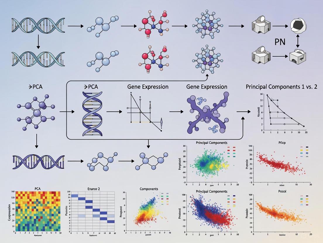
Figure 1: The conceptual workflow of how PCA scores are generated and used. Samples are transformed from a high-dimensional gene space to a low-dimensional PCA space for easier visualization and interpretation.
Loadings
Loadings (or eigenvectors) are the weights assigned to each original variable (gene) in a principal component [14] [17]. They define the direction of the PC in the original high-dimensional space.
- Mathematical Definition: Loadings are the eigenvectors of the covariance matrix. Each loading vector is a unit vector, and all loading vectors are mutually orthogonal [18] [8].
- Geometric Interpretation: A loading value is the cosine of the angle between the original variable's axis and the principal component axis [17]. A loading close to +1 or -1 indicates the variable strongly influences that PC's direction. The sign indicates whether the variable's contribution is positive or negative [17].
- Interpretation: Genes with high absolute loadings on a PC are the major drivers of the variance that PC captures. Analyzing these top-loading genes can provide biological meaning to a component (e.g., revealing that PC1 represents a gene signature related to cellular proliferation) [14].
Table 2: Interpreting PCA Loadings for a Hypothetical 2-Gene System
| Original Variable | Loading on PC1 | Interpretation |
|---|---|---|
| Gene A | 0.500 | Gene A contributes positively to PC1. Its influence is moderate. |
| Gene B | 0.866 | Gene B contributes positively to PC1. It is a stronger driver of PC1 than Gene A. |
The loadings show that PC1 is more aligned with the direction of Gene B, which has a higher loading value [17].
Protocols for Projecting Gene Expression Data onto Principal Components
This protocol details the steps for performing PCA on gene expression data, from preprocessing to projection and validation.
Data Preprocessing and Normalization
The choice of normalization method profoundly impacts the correlation structure of the data and, consequently, the PCA model and its biological interpretation [21].
- Step 1: Data Matrix Construction: Create a genes-by-samples matrix of expression values (e.g., FPKM, TPM, or normalized counts from RNA-seq).
- Step 2: Normalization: Apply a robust normalization method to remove technical artifacts. A comprehensive evaluation of 12 methods showed that the choice of normalization affects gene ranking and pathway interpretation in PCA [21]. Methods like TMM (Trimmed Mean of M-values) or DESeq2's median-of-ratios are common starting points.
- Step 3: Transformation and Scaling: For gene expression data, a log₂ transformation is often applied to stabilize variance. Centering (subtracting the column mean) is essential for PCA. Scaling (dividing by the column standard deviation) to unit variance is recommended if genes are on different scales, to prevent high-expression genes from dominating the model [16] [15].
PCA Computation and Projection
The core computational process can be efficiently performed in R using the prcomp() function.
- Step 1: Compute PCA: Use
pca_result <- prcomp(t(expression_matrix), center = TRUE, scale. = TRUE). Transposing the matrix ensures samples are rows and genes are columns, as required byprcomp[16]. - Step 2: Extract Outputs:
- Scores:
pca_scores <- pca_result$x - Loadings:
pca_loadings <- pca_result$rotation - Standard Deviations:
pca_sdev <- pca_result$sdev - Variances:
eigenvalues <- (pca_result$sdev)^2[16]
- Scores:
- Step 3: Project Data: The projection is performed automatically during the
prcomp()call. The scores are the result of the matrix multiplication:Scores = Scaled_Data × Loadings[8].
Figure 2: A streamlined workflow for performing Principal Component Analysis on gene expression data, from raw input to interpretable output.
Validation of the PCA Model
Before biological interpretation, validating that the PCA model is robust and describes intended biology is critical, especially when applying a pre-defined gene signature to a new dataset [14].
- Coherence: Assess if genes within the signature are correlated beyond chance in the target dataset. This can be done by comparing the variance explained by the signature's first PC to that of thousands of randomly generated gene sets [14].
- Uniqueness: Ensure the signature's primary signal is not merely a reflection of a dominant, general direction in the data (e.g., a proliferation bias in tumor datasets). The signature's first PC should be distinguishable from the first PC of the entire transcriptome [14].
- Robustness: The biological signal should be strong and distinct. This can be tested by evaluating the variance captured in the first PC relative to the second; a sharp drop (as seen in a scree plot) indicates a strong, dominant signal [14] [18].
- Transferability: The PCA-based gene signature score must describe the same biology in the target dataset as in the training dataset. This involves checking the correlation of loadings or the biological function of top-loading genes [14].
The Scientist's Toolkit: Research Reagent Solutions
Table 3: Essential Computational Tools for PCA in Gene Expression Analysis
| Tool / Resource | Function | Application Note |
|---|---|---|
| R Statistical Environment | Open-source platform for statistical computing and graphics. | The primary environment for running PCA and downstream analyses. |
| prcomp() / PCA() functions | Core R functions for performing PCA. | prcomp() is preferred for numerical accuracy using SVD [16]. |
| MDAnalysis Python Toolkit | Object-oriented toolkit for analyzing molecular dynamics trajectories. | Can be adapted for analysis of protein dynamics from structural data [20]. |
| VolSurf+ | Mathematical platform for computing molecular descriptors from 3D structures. | Used to derive descriptors for permeability and solubility in drug discovery [11]. |
Application Example: PCA in Neuroprotective Drug Discovery
A study on quercetin analogues aimed to identify compounds with improved blood-brain barrier (BBB) permeability used PCA to identify key molecular descriptors [11].
- Objective: Understand which molecular descriptors (e.g., logP, solubility parameters) primarily govern BBB permeation in a set of 34 quercetin analogues.
- Method: PCA was applied to a matrix of multiple computed molecular descriptors for all analogues. The resulting scores and loadings were analyzed.
- Result: The PCA model successfully reduced the descriptor space. The first few PCs captured the majority of the variance. Analysis of loadings revealed that descriptors related to intrinsic solubility and lipophilicity (logP) were the main drivers of the first principal components, meaning they were most responsible for the clustering pattern seen in the scores plot [11].
- Conclusion: This PCA output provided a clear, data-driven direction for future synthetic efforts: focus on modifying analogues to optimize lipophilicity and solubility to enhance BBB penetration [11].
Interpreting PCA outputs is a critical skill for extracting meaningful biological insights from high-dimensional gene expression data. A rigorous approach involves not just visualizing sample scores for clusters, but also quantitatively assessing the variance explained to determine the significance of components and interrogating the loadings to assign biological meaning to the patterns observed. By following the standardized protocols for projection and validation outlined in this guide, researchers can ensure their PCA models are robust, reproducible, and truly reflective of underlying biology, thereby reliably informing subsequent drug discovery and development decisions.
In the analysis of high-dimensional genomic data, exploratory techniques are not merely a preliminary step but a critical foundation for ensuring robust and biologically meaningful conclusions. Gene expression studies, characterized by their "large d, small n" paradigm (a large number of genes profiled over a relatively small number of samples), present unique challenges in visualizing data structure and identifying anomalous observations [1]. This document, framed within a broader thesis on projecting gene expression data onto principal components, outlines detailed application notes and protocols for key exploratory analyses. We focus on the pivotal roles of Principal Component Analysis (PCA) for visualizing sample similarity and multivariate methods for detecting outliers, providing scientists and drug development professionals with the practical toolkit necessary to navigate the complexity of transcriptomic data.
Principal Component Analysis: A Dimensionality Reduction Powerhouse
Core Concepts and Rationale
Principal Component Analysis (PCA) is a classic dimension reduction approach that constructs new, uncorrelated variables called principal components (PCs), which are linear combinations of the original gene expressions [1]. The core objective is to project high-dimensional data into a lower-dimensional space while preserving the maximal amount of variance. This is achieved by identifying axes of greatest variance (principal components), where the first PC captures the most variation, the second PC (orthogonal to the first) captures the next most, and so on [22].
In the context of bioinformatics, the first few PCs are assumed to capture dominant biological signals and major factors of heterogeneity, whereas later PCs are often associated with random technical or biological noise [22]. This makes PCA invaluable for data compaction, noise reduction, and the generation of intuitive visualizations that reveal underlying sample relationships.
Quantitative and Qualitative Applications in Genomics
PCA serves multiple critical functions in genomic data analysis:
- Exploratory Analysis and Data Visualization: It enables the projection of thousands of dimensional gene expressions onto a 2- or 3-dimensional space (e.g., PC1 vs. PC2), allowing researchers to visually assess sample clustering, identify batch effects, and observe broad patterns [1] [23].
- Clustering Analysis: The first few PCs, which capture most of the variation, can be used as input for clustering genes or samples, offering a denoised representation of the data [1].
- Regression Analysis: In studies aiming to predict clinical outcomes, the top PCs can be used as covariates in regression models, effectively circumventing the high-dimensionality problem and avoiding collinearity [1].
Visualizing Sample Similarity through PCA and Clustering
Assessing how samples relate to each other—whether replicates are consistent or treatment groups are distinct—is a fundamental question in genomics [24]. PCA is an intuitive way to identify sample clusters in a reduced-dimensionality plot [23].
Protocol: Sample Similarity Analysis via PCA
Objective: To reduce the dimensionality of a gene expression matrix and visualize sample relationships based on principal components. Input: A normalized gene expression matrix (e.g., log-counts) with rows representing genes and columns representing samples.
- Feature Selection: Select a subset of genes for PCA to reduce noise and computational load. Typically, this involves using the top 2000 genes with the highest biological variance (e.g., highly variable genes, or HVGs) [22].
- Data Scaling: Standardize the expression values for each gene to a mean of zero and a standard deviation of one (z-scores). This ensures that genes with high expression levels do not dominate the variance calculation simply due to their scale [24].
- PCA Computation: Perform PCA on the scaled and subsetted expression matrix using a singular value decomposition (SVD) algorithm. By default, the first 50 PCs are often computed and stored [22].
- Determination of PCs: Choose the number of top principal components (d) to retain for downstream analysis. While this can be data-driven, a common practice is to use an arbitrary but reasonable number, often between 10 and 50, as the later PCs explain minimal variance [22].
- Visualization: Create a scatter plot of the samples using the first two (or three) PCs. Samples with similar gene expression profiles will cluster together in this projected space [22].
Complementary Technique: Hierarchical Clustering
An alternative or complementary method for assessing sample similarity is hierarchical clustering, which creates a tree structure (dendrogram) showing the relationship between individual data points and clusters [24].
Protocol: Hierarchical Clustering of Samples
- Distance Calculation: Compute a distance matrix between all pairs of samples. Common metrics include Euclidean distance or correlation distance (
1 - correlation coefficient) [24]. - Clustering Algorithm: Perform hierarchical clustering on the distance matrix using a linkage method. "Ward's minimum variance method" is often recommended as it aims to find compact, spherical clusters [24].
- Visualization: Visualize the results as a dendrogram and often in tandem with a heatmap, which color-codes the original expression values to reveal patterns driving the cluster formation [24].
Table 1: Common Distance Metrics for Sample Clustering
| Metric Name | Formula | Use Case and Properties |
|---|---|---|
| Euclidean Distance | d_AB = √[Σ(e_Ai - e_Bi)²] |
The default "ordinary" distance; can be heavily influenced by outliers [24]. |
| Manhattan Distance | d_AB = Σ|e_Ai - e_Bi| |
Less sensitive to outliers compared to Euclidean distance [24]. |
| Correlation Distance | d_AB = 1 - ρ (ρ = Pearson correlation) |
Measures similarity in expression pattern, independent of scale [24]. |
Detecting Multivariate Outliers
In high-dimensional data, an outlier may not be extreme in any single dimension but can be an unusual combination of multiple variables [25]. These multivariate outliers can heavily influence model fitting and lead to incorrect biological inferences.
Protocol: Multivariate Outlier Detection using Mahalanobis Distance
Objective: To identify samples that are multivariate outliers based on their principal component scores. Input: The matrix of principal component scores from the PCA analysis (typically the top d PCs).
- Calculate Mahalanobis Distance: For each sample, compute the Mahalanobis distance of its PC score vector from the centroid of all sample scores. The Mahalanobis distance accounts for the covariance structure of the data, unlike Euclidean distance [25] [26].
- Assess Statistical Significance: Compare the calculated Mahalanobis distances to a Chi-square (χ²) distribution. The degrees of freedom (df) for this distribution are equal to the number of PCs used in the calculation [26].
- Identify Outliers: Compute the right-tail p-value for each distance (
1 - CDF.CHISQ(mahal_dist, df)). Samples with a p-value below a significance threshold (e.g., .001) are flagged as potential multivariate outliers [26].
Alternative Outlier Detection Methods
While Mahalanobis distance is a common parametric approach, other powerful methods exist.
Table 2: Methods for Multivariate Outlier Detection
| Method | Brief Description | Key Considerations |
|---|---|---|
| Mahalanobis Distance | Measures the distance of a point from the data centroid, accounting for covariance [25] [26]. | Sensitive to the presence of outliers itself, as they can distort the mean and covariance estimates. |
| Robust Mahalanobis | Uses robust estimates of the centroid and covariance matrix (e.g., minimum covariance determinant) [25]. | More reliable for outlier detection as it is less influenced by the outliers themselves. |
| Principal Component Analysis (PCA) | Visually inspect the first few PCs for samples that lie far from the main cloud of data [27]. | A simple, intuitive approach, but may miss outliers that do not manifest in the first two PCs. |
| Isolation Forest | A model-based method that isolates anomalies by randomly selecting features and split values [27]. | Effective for high-dimensional data and does not rely on assumptions of data distribution. |
The Scientist's Toolkit: Essential Research Reagents and Computational Solutions
Table 3: Key Research Reagent Solutions for Exploratory Analysis
| Item / Software Package | Function in Analysis |
|---|---|
| R Statistical Environment | A comprehensive platform for statistical computing and graphics. The prcomp function is a standard tool for performing PCA [1]. |
| scran / scater (R/Bioconductor) | Specialized packages for single-cell RNA-seq data analysis. They provide optimized functions like fixedPCA() for efficient and scalable PCA computation [22]. |
| Python (scikit-learn) | A general-purpose programming language with extensive data science libraries. sklearn.decomposition.PCA is a widely used implementation of PCA [28]. |
| Mahalanobis Distance (in R/SPSS) | A statistical distance metric used for multivariate outlier detection. Can be computed in R via mahalanobis() or in SPSS via the Linear Regression menu with the "Save Mahalanobis distances" option [26]. |
| Hierarchical Clustering (hclust in R) | A standard function for performing hierarchical cluster analysis on a distance matrix, essential for generating dendrograms of sample relationships [24]. |
| Heatmap Visualization (pheatmap in R) | A function for drawing annotated heatmaps, often combined with clustering to visualize gene expression patterns across samples [24]. |
A Step-by-Step Pipeline: Executing PCA on Your Gene Expression Matrix
In gene expression analysis, techniques like RNA-sequencing (RNA-seq) and microarrays generate high-dimensional data where the number of measured genes (variables, P) vastly exceeds the number of biological samples (observations, N). This structure, often called a "P ≫ N" scenario, presents significant challenges for analysis and visualization due to the curse of dimensionality [7]. Principal Component Analysis (PCA) is a powerful unsupervised machine learning method essential for exploring such data, revealing patterns, identifying outliers, and visualizing sample relationships [21] [29] [30]. The accuracy and biological interpretability of PCA, however, are profoundly influenced by how the raw count matrix is prepared and normalized prior to analysis. This protocol details the critical steps for structuring a gene expression count matrix—with samples as rows and genes as columns—to ensure robust and meaningful PCA outcomes within a gene expression research thesis.
Background & Key Concepts
The Curse of Dimensionality in Transcriptomic Data
Transcriptomic datasets commonly profile the expression of over 20,000 genes (P) across fewer than 100 samples (N). In this high-dimensional space, data points become sparse, making analysis and visualization computationally challenging and mathematically unstable. Dimensionality reduction techniques like PCA are essential to mitigate these effects [7].
The Role of PCA in Gene Expression Analysis
PCA transforms the original high-dimensional data into a new set of uncorrelated variables, the principal components (PCs), which are linear combinations of the original genes. The first PC captures the direction of maximum variance in the data, with each subsequent component capturing the next highest variance under the constraint of orthogonality [31] [30]. This transformation is pivotal for:
- Exploratory Data Analysis (EDA): Assessing data quality, identifying batch effects, and detecting sample outliers [21] [29].
- Visualization: Projecting samples into a 2D or 3D space defined by the top PCs to visualize inherent clustering or trends [30] [32].
- Downstream Analysis: Providing a de-noised, lower-dimensional representation for clustering or as input to non-linear dimensionality reduction techniques like t-SNE and UMAP [29] [32].
Experimental Protocol: Data Preparation Workflow
The following workflow outlines the standardized procedure for preparing a gene expression count matrix for PCA. The accompanying diagram visualizes this multi-stage process.
Protocol 3.1: Data Curation and Initial Quality Control
Objective: To filter the raw count matrix for low-quality samples and uninformative genes.
- Remove Low-Quality Samples: Calculate the total library size (sum of counts) per sample. Exclude samples with an extremely low library size, which may indicate failed libraries. The specific threshold is experiment-dependent.
- Filter Lowly Expressed Genes: Remove genes with zero or near-zero counts across the majority of samples. A common filter is to keep only genes with a count per million (CPM) above a threshold (e.g., 1 CPM) in at least
nsamples, wherenis the size of the smallest experimental group. - Address Missing Data: Identify genes with missing values. Common strategies include imputation using methods like
scikit-learn'sSimpleImputeror removal of genes with excessive missingness.
Protocol 3.2: Data Normalization
Objective: To remove technical variation (e.g., sequencing depth, sample-specific biases) while preserving biological signal.
Normalization is a critical step, and the choice of method can significantly impact the PCA results and their biological interpretation [21]. The table below summarizes common and advanced methods.
Table 1: Overview of Gene Expression Data Normalization Methods
| Method Category | Specific Method | Key Principle | Suitability for PCA |
|---|---|---|---|
| Library Size Scaling | Total Count | Scales counts by total library size per sample. | Basic method; can be confounded by highly expressed genes. |
| Reference Gene-Based | Housekeeping Genes [33] | Uses stably expressed internal reference genes for scaling. | Dependent on validated, stable reference genes for the tissue/condition. |
| Global Mean (GM) [33] | Uses the global mean expression of all profiled genes as a baseline. | Effective when profiling >55 genes; outperforms multiple RGs in some studies [33]. | |
| Non-Differentially Expressed Genes (NDEG) [34] | Uses genes identified as statistically non-differential (high p-value from ANOVA) for scaling. | Improves cross-platform (microarray/RNA-seq) model performance [34]. | |
| Statistical Modeling | SCTransform | Uses a regularized negative binomial model. | May remove spatial domain signals in spatial transcriptomics [35]. |
| Spatially-Aware | SpaNorm [35] | A GLM-based method that concurrently models and segregates library size effects from biology using spatial information. | Superior for spatial transcriptomics; retains spatial domain information and improves SVG detection [35]. |
Procedure:
- Select a Method: Choose a normalization method appropriate for your data type (e.g., bulk RNA-seq, spatial transcriptomics) and experimental design.
- Apply Normalization: Use dedicated software packages (e.g.,
scikit-learn,Rpackages, or specialized tools like SpaNorm) to apply the chosen normalization, transforming the raw count matrix.
Protocol 3.3: Feature Selection for Dimensionality Reduction
Objective: To reduce noise and computational load by selecting a subset of informative genes for PCA.
- Variance-Based Selection: A common approach is to select the top
Ngenes (e.g., 1000-5000) with the highest variance across samples. This targets genes that are most likely to contribute to the separation of samples in the PCA space. - Differentially Expressed Genes (DEGs): Alternatively, use statistical tests (e.g., ANOVA [34]) to identify genes significantly associated with the experimental conditions. Using DEGs for PCA can sharpen the separation of pre-defined groups.
Protocol 3.4: Data Scaling
Objective: To standardize the data so that each gene contributes equally to the PCA, preventing highly expressed genes from dominating the principal components.
- Standardization (Z-score): For each gene, subtract the mean expression and divide by the standard deviation. This results in all genes having a mean of 0 and a standard deviation of 1.
- Implementation: Use
StandardScalerfromscikit-learn.
- Implementation: Use
- Apply Scaling: Fit the scaler on the normalized and filtered matrix and transform the data. The output is the final, pre-processed matrix ready for PCA.
The Scientist's Toolkit
Table 2: Essential Research Reagents and Computational Tools
| Item / Software | Function / Purpose | Example / Note |
|---|---|---|
| Reference Genes (RGs) | Endogenous controls for normalizing qPCR or RNA-seq data. | Must be validated for stability. RPS5, RPL8, HMBS are stable in canine GI tissue [33]. |
| Non-Differentially Expressed Genes (NDEGs) | A set of stable genes identified from the dataset itself for normalization. | Selected based on high p-value (e.g., p>0.85) from ANOVA [34]. |
| scikit-learn (Python) | A comprehensive machine learning library. | Provides PCA, StandardScaler, and various utilities for the entire workflow. |
| Single-Cell / Spatial Packages | Specialized tools for modern transcriptomics data. | scran [35] for scRNA-seq; SpaNorm [35] for spatial transcriptomics. |
| Stable Algorithms (e.g., IRLBA) | Memory-efficient and fast PCA implementations for large datasets. | Crucial for large-scale single-cell RNA-sequencing data [29]. |
Anticipated Results and Interpretation
After applying PCA to the prepared matrix, the following outputs are standard:
- Explained Variance Ratio: The proportion of the total variance captured by each principal component. This is used to determine the number of components to retain, often by looking for an "elbow" in a scree plot or by retaining enough components to explain a set threshold (e.g., 95%) of the variance [31] [30].
- PCA Loadings: The coefficients (
pca.components_inscikit-learn) representing the contribution of each original gene to each principal component. High-loading genes drive the separation seen along that PC and can be biologically interpreted. - PCA Scores: The coordinates of the samples in the new PC space (
pca.transform()). These are plotted to visualize sample clustering.
A well-prepared matrix should yield a PCA plot where biological replicates cluster together, and separation between experimental groups aligns with the hypothesis. Conversely, strong batch effects or clustering driven by technical artifacts indicates potential issues with the normalization or data curation steps.
In the analysis of high-dimensional gene expression data, Principal Component Analysis (PCA) serves as a fundamental technique for exploratory data analysis and visualization. The reliability of its output, however, is profoundly dependent on appropriate data preprocessing. Normalization, scaling, and centering are not merely optional steps but critical transformations that determine whether PCA reveals true biological signals or amplifies technical artifacts and noise. This application note examines the impact of these preprocessing steps within the context of projecting gene expression data onto principal components, providing structured protocols and analyses for research scientists and drug development professionals.
Research demonstrates that although PCA score plots may appear similar across different normalization methods, the biological interpretation of these models can vary dramatically based on the preprocessing approach used [21]. Without proper centering, PCA captures variance around zero instead of the mean expression, causing highly expressed housekeeping genes to dominate the first principal component regardless of their biological relevance to the experimental conditions [36]. Similarly, without scaling, genes with large numeric ranges and high expression levels can disproportionately influence the analysis, potentially obscuring more meaningful but subtle expression patterns [36].
Background and Key Concepts
The Curse of Dimensionality in Gene Expression Data
Gene expression data from technologies like RNA-sequencing typically manifests in a classic high-dimensional structure where the number of variables (genes, P) vastly exceeds the number of observations (samples, N). It is common to analyze more than 20,000 genes across fewer than 100 samples, creating significant computational and statistical challenges for visualization, analysis, and mathematical operations [7]. This "curse of dimensionality" necessitates effective dimensionality reduction strategies like PCA to make biological interpretation feasible.
The Mathematics of PCA and Preprocessing
PCA operates by identifying orthogonal directions of maximal variance in the dataset, with the first principal component capturing the greatest variance, the second the next greatest, and so on [37]. The algorithm is sensitive to the scale and distribution of variables, making preprocessing decisions fundamental to its output:
- Centering involves subtracting the mean expression of each gene across all samples. This ensures that PCA measures variance around the mean expression rather than around zero, preventing highly expressed genes from dominating components simply due to their abundance rather than biologically relevant variation [36].
- Scaling standardizes the variance of each gene, typically by dividing by the standard deviation after centering (Z-scoring). This gives equal weight to all genes in the analysis, preventing those with naturally large expression ranges from overwhelming the variance structure [36].
Table 1: Critical Preprocessing Steps for PCA
| Processing Step | Mathematical Operation | Impact on PCA | When to Use |
|---|---|---|---|
| Centering | Subtract gene-wise mean | Shifts focus from mean expression to variation around mean | Almost always for gene expression |
| Scaling (Z-score) | (Value - Mean)/Standard Deviation | Equalizes influence of all genes regardless of expression level | When comparing expression patterns across genes |
| Library Size Normalization | Adjust for total sequencing depth (e.g., TMM, CPM) | Enables cross-sample comparison by removing technical variation | Essential for RNA-seq data before centering and scaling |
Normalization Methods for RNA-Seq Data
RNA-sequencing data requires specialized normalization to address technical artifacts including sequencing depth and library composition before conducting PCA. The raw count matrix generated from RNA-seq processing cannot be directly compared between samples because the number of reads mapped to a gene depends not only on its expression level but also on the total number of sequencing reads obtained for that sample [38].
Common Normalization Techniques
- Counts Per Million (CPM): A simple normalization where raw read counts for each gene are divided by the total number of reads in the library, then multiplied by one million. This method corrects for sequencing depth but remains sensitive to highly expressed genes that consume a large fraction of reads [38].
- Trimmed Mean of M-values (TMM): A more sophisticated method that uses a weighted trimmed mean of the log expression ratios to account for differences in library composition [39]. TMM normalization specifically addresses situations where a few highly expressed genes in one condition can skew the representation of other genes [39] [40].
- Median-of-Ratios: Used in DESeq2, this method calculates a reference expression level for each gene and then a size factor for each sample to adjust for sequencing depth while considering library composition [38].
Impact on Downstream PCA
Different normalization methods directly impact the PCA results and their biological interpretation. A comprehensive evaluation of 12 normalization methods for transcriptomics data found that although PCA score plots often appear similar regardless of normalization, the biological interpretation of the models depends heavily on the method applied [21]. Specifically, the choice of normalization affects:
- Model complexity in PCA
- Quality of sample clustering in low-dimensional space
- Gene ranking in the model fit
- Pathway enrichment results during biological interpretation [21]
Table 2: Comparison of RNA-Seq Normalization Methods for PCA
| Method | Sequencing Depth Correction | Library Composition Correction | Impact on PCA | Best Use Cases |
|---|---|---|---|---|
| CPM | Yes | No | May be dominated by highly expressed genes; can distort sample relationships | Initial exploration, but not recommended for final analysis |
| TMM | Yes | Yes | Reduces composition bias; improves biological signal recovery | Differential expression analysis; multi-tissue comparisons [40] |
| Median-of-Ratios | Yes | Yes | Robust to expression shifts; improves cluster separation | Differential expression analysis with DESeq2 |
| TPM | Yes | Partial | Adjusts for gene length; reduces composition bias | Within-sample comparisons and visualizations |
Experimental Protocols
Comprehensive Workflow for RNA-Seq Normalization and PCA
The following workflow outlines a robust methodology for preprocessing RNA-seq data prior to PCA, incorporating quality control, normalization, and batch effect correction.
Workflow: RNA-Seq Preprocessing for PCA
Protocol 1: TMM Normalization with Centering and Scaling
This protocol details the specific steps for implementing TMM normalization followed by centering and scaling prior to PCA, adapted from the GTEx_Pro pipeline [40].
Materials and Reagents
- Raw count matrix from RNA-seq alignment/quantification
- R statistical software (version 4.0 or higher)
- edgeR package for TMM normalization
- Metadata file containing sample information
Methodology
Data Input and Filtering
- Import raw count data into R using
read.table()orfread() - Filter out genes with low expression: Remove genes with counts per million (CPM) < 1 in at least X samples, where X equals the smallest group size
- This step reduces noise and computational complexity
- Import raw count data into R using
TMM Normalization
- Create a DGEList object using
edgeR::DGEList() - Calculate normalization factors:
calcNormFactors(object, method = "TMM") - The TMM method trims extreme log-fold-changes and absolute expression levels (default: trim 30% of M values and 5% of A values) to robustly estimate scaling factors [39]
- Create a DGEList object using
CPM Transformation
- Apply
edgeR::cpm()function with log = FALSE to convert normalized counts to counts per million scale - This standardizes for sequencing depth across samples
- Apply
Batch Effect Correction (Optional but Recommended)
- Identify batch effects using surrogate variable analysis (SVA) with the
svapackage - Include known batch variables and surrogate variables in the normalization model
- The GTEx_Pro pipeline demonstrated that SVA following TMM+CPM normalization substantially improves tissue-specific clustering in PCA [40]
- Identify batch effects using surrogate variable analysis (SVA) with the
Centering and Scaling
- Center the data: Subtract the mean expression for each gene across all samples
- Scale the data: Divide by the standard deviation for each gene
- This can be accomplished in R using the
scale()function
Principal Component Analysis
- Perform PCA using the
prcomp()function in R - Visualize results using score plots and loading plots
- Evaluate the proportion of variance explained by each component
- Perform PCA using the
Protocol 2: Evaluation of Normalization Impact
This protocol provides a systematic approach to evaluate how different normalization methods affect PCA outcomes.
Experimental Design
- Apply multiple normalization methods (CPM, TMM, Median-of-Ratios) to the same raw count matrix
- Perform PCA on each normalized dataset
- Compare results using both quantitative metrics and qualitative assessments
Evaluation Metrics
Cluster Quality Metrics
- Calculate the Davies-Bouldin Index (DBI) to assess separation and compactness of sample clusters in PCA space
- Lower DBI values indicate better clustering [40]
Variance Explained
- Compare the proportion of variance captured by the first several principal components across normalization methods
- Note that normalization often reduces the total variance explained by early PCs by diminishing the influence of technical artifacts
Biological Concordance
- Assess whether known biological groups (e.g., tissue types, treatment conditions) separate appropriately in PCA space
- Validate with established housekeeping genes and tissue-specific markers [40]
Case Study: Multi-Tissue Gene Expression Analysis
The GTEx_Pro pipeline provides a compelling case study on the importance of robust normalization for PCA of gene expression data across multiple tissues [40].
Methods and Implementation
Researchers analyzed GTEx v8 RNA-sequencing data comprising 54 tissues with 17,235 total samples. The pipeline implemented:
- TMM + CPM normalization to address library size differences and compositional biases
- Surrogate Variable Analysis (SVA) to correct for batch effects related to donor demographics and tissue processing
- PCA to visualize sample relationships before and after processing
Results and Interpretation
- Raw Data PCA: 3D PCA of raw count data showed substantial overlap between different tissues, with clustering driven primarily by technical variation rather than biological signal [40]
- After TMM + CPM Normalization: PCA revealed pronounced tissue-specific clustering, with biologically related tissues (e.g., heart chambers, skin regions) grouping together
- After SVA Correction: Further improvement in tissue separation with increased Euclidean distances between distinct tissue clusters
- Quantitative Improvement: The Davies-Bouldin index decreased after SVA correction, indicating better clustering quality, while overall variance in the first two principal components increased by 1.5% [40]
The Scientist's Toolkit
Table 3: Essential Tools for RNA-Seq Normalization and PCA
| Tool/Resource | Function | Application Context |
|---|---|---|
| edgeR | TMM normalization implementation | RNA-seq data normalization prior to differential expression and PCA |
| DESeq2 | Median-of-ratios normalization | Alternative normalization approach with robust composition adjustment |
| SVA Package | Batch effect correction | Identifying and adjusting for surrogate variables representing batch effects |
| FastQC | Quality control assessment | Initial evaluation of raw sequencing data quality |
| GTEx_Pro Pipeline | Integrated normalization workflow | Comprehensive processing for multi-tissue gene expression data [40] |
Preprocessing decisions, particularly normalization, centering, and scaling, fundamentally shape the results of Principal Component Analysis for gene expression data. The systematic evaluation of normalization methods demonstrates that while visual similarities may exist in PCA projections across methods, the biological interpretation varies significantly [21]. Researchers should select normalization approaches based on their specific data characteristics and biological questions, implement careful centering and scaling to focus on biologically relevant variation, and always validate their preprocessing choices through quantitative metrics and biological plausibility checks. The provided protocols offer a robust foundation for generating reliable, interpretable PCA results from high-dimensional gene expression data.
Principal Component Analysis (PCA) is a foundational dimensionality reduction technique in computational biology, indispensable for analyzing high-dimensional gene expression data. By transforming vast datasets into a lower-dimensional space defined by principal components, PCA facilitates the identification of patterns, outliers, and key sources of biological variation. This protocol provides a detailed, step-by-step guide for implementing PCA in R using the prcomp() function, with a specific focus on applications in genomic research. We cover the complete workflow—from data preprocessing and model fitting to the interpretation and projection of new data—enabling researchers and drug development professionals to efficiently extract meaningful insights from complex transcriptomic profiles.
The analysis of gene expression data, such as from RNA-seq experiments, presents a classic challenge of high dimensionality. A typical dataset contains expression levels for thousands of genes (variables, P) across far fewer samples or cells (observations, N), a scenario often described as the "curse of dimensionality" [7]. This P≫N situation complicates visualization, increases computational cost, and risks model overfitting.
PCA addresses this by performing a linear transformation of the original correlated variables (gene expression levels) into a new set of uncorrelated variables called principal components (PCs). These PCs are ordered such that the first few capture the greatest proportion of variance present in the original dataset [37]. In genomics, this allows researchers to:
- Visualize major sample groupings or gradients (e.g., by cell type, treatment, or disease state) in 2D or 3D plots.
- Identify technical artifacts or batch effects that dominate data variance.
- Reduce noise by focusing downstream analyses (like clustering) on the most informative components.
- Prepare data for further machine learning tasks by creating a lower-dimensional, denoised representation.
The prcomp() function in R is a preferred method for PCA due to its numerical stability, ease of use, and direct integration into the bioinformatics ecosystem [41] [42].
Materials: The Researcher's Toolkit
Software and Computing Environment
| Resource | Specification | Function |
|---|---|---|
| R Programming Language | Version 4.0.0 or higher | Provides the core computational environment for statistical analysis and execution of the prcomp() function [41]. |
| RStudio IDE | (Recommended) | Offers an integrated development environment for R, facilitating script writing, visualization, and data management. |
| Core R Packages | stats (includes prcomp) |
Performs the principal component analysis [41] [42]. |
| Visualization Packages | ggplot2, factoextra |
Creates high-quality static plots, including scree plots and PCA scatter plots [43]. |
| Hardware | Minimum 8GB RAM | Sufficient memory is critical for handling large gene expression matrices, which can exceed several gigabytes in size. |
Data Requirements
A gene expression data matrix is the primary input. The data should be structured as an N x P matrix, where rows (N) represent individual observations (e.g., cells, patient samples), and columns (P) represent variables (e.g., measured gene expression levels) [7]. The matrix must contain numeric values only (e.g., normalized read counts, FPKM, TPM). Categorical metadata (e.g., sample species, treatment group) is stored separately and used for coloring points in visualizations.
Methodology
The following diagram illustrates the complete PCA workflow for gene expression analysis, from raw data to the projection of new samples.
Protocol: A Step-by-Step Guide
This section provides a detailed, hands-on protocol for performing PCA on a typical gene expression dataset.
Step 1: Data Preprocessing and Preparation
Proper preprocessing is critical for a biologically meaningful PCA.
Load Data: Begin by reading your gene expression matrix into R. The matrix should have genes as columns and samples as rows.
Subset and Clean: Ensure the data contains only numeric values. Remove any non-numeric columns (e.g., gene symbols should be row names, not a separate column).
Center and Scale: Center the data (subtract the mean of each gene) to ensure the first PC captures the direction of maximum variance, not the mean. Scaling (dividing by the standard deviation of each gene) is equally important, as it gives all genes equal weight. This prevents highly expressed genes from dominating the PCs purely due to their magnitude [43].
Step 2: Performing PCA withprcomp()
Execute the PCA using the prcomp() function from the stats package.
Note: The center and scale. parameters are set to FALSE because we have already performed these operations in the previous step [41].
Step 3: Interpreting the PCA Output
The pca_result object contains several key elements [41]:
sdev: The standard deviations of the principal components. Squaring these gives the eigenvalues (variances).rotation: The matrix of variable loadings (eigenvectors). Each column corresponds to a PC and indicates the contribution (weight) of each original gene to that PC.x: The coordinates of the original data projected into the principal component space (the PCA scores).
Use summary() to obtain a quick overview of the importance of each component.
The following table quantifies the importance of the first five principal components from a hypothetical gene expression analysis, showing the cumulative variance reaching over 80%.
Table 1: Importance of Principal Components in a Hypothetical Gene Expression Dataset
| Principal Component | Standard Deviation | Proportion of Variance | Cumulative Proportion |
|---|---|---|---|
| PC1 | 1.1077 | 0.2454 | 0.2454 |
| PC2 | 1.0610 | 0.2251 | 0.4705 |
| PC3 | 1.0191 | 0.2077 | 0.6783 |
| PC4 | 0.9468 | 0.1793 | 0.8575 |
| PC5 | 0.8440 | 0.1425 | 1.0000 |
Step 4: Visualizing the Results
Effective visualization is key to interpreting PCA.
Scree Plot: This plot displays the variances (eigenvalues) associated with each PC. It helps determine the number of meaningful components to retain, typically by looking for an "elbow" point where the variance levels off [43].
PCA Scores Plot: The most common visualization, showing samples projected onto the first two PCs. Coloring points by metadata (e.g., cell type) can reveal biological clusters.
Biplot: Overlays the scores plot with arrows representing the loadings of genes, showing how genes contribute to the sample separation seen in the plot [43].
Step 5: Projecting New Data onto the PCA Space
To project new, unseen gene expression data (e.g., a validation cohort) onto the existing PCA axes, use the rotation matrix from the original prcomp fit [41].
The logic of projecting new data is summarized in the diagram below, which ensures the new samples are transformed in a manner consistent with the original model.
Troubleshooting and Best Practices
- Data Quality: PCA is sensitive to outliers. Extreme values can distort the principal components. Perform exploratory data analysis to detect and address outliers before PCA.
- Scaling is Crucial: For gene expression data, where the dynamic range of different genes can vary drastically, scaling is non-optional. Without it, the analysis will be biased towards highly variable genes.
- Interpreting Loadings: To identify genes driving variation along a specific PC, examine the
rotationmatrix. Genes with large absolute values in a specific PC's column have a strong influence on that component. - Advanced Methods: For very large or sparse single-cell RNA-seq data, consider advanced variants like Sparse PCA, which forces some loadings to zero, enhancing interpretability [44].
Applications in Genomic Research
PCA is a versatile tool used across genomic studies. It is routinely applied to:
- Quality Control: Identify batch effects or outlier samples in transcriptomic studies.
- Cell Type Identification: Visualize and identify clusters of cells in single-cell RNA sequencing (scRNA-seq) data [45] [44].
- Disease Subtyping: Discover novel molecular subtypes of cancer or other complex diseases by identifying sample clusters in PC space associated with clinical outcomes.
- Integrative Multi-omics: Serve as a foundational step in integrating multiple data types (e.g., genomics, transcriptomics, proteomics) for a unified analysis [46] [47].
This protocol has outlined a comprehensive workflow for performing Principal Component Analysis using R's prcomp() function in the context of gene expression data. By following these detailed steps—from rigorous data preprocessing and model fitting to insightful visualization and new data projection—researchers can effectively reduce the dimensionality of complex genomic datasets. This process unveils underlying biological structures, facilitates quality control, and provides a solid foundation for further statistical analysis and machine learning, thereby accelerating discovery in genomics and drug development.
Principal Component Analysis (PCA) is an unsupervised linear dimension reduction method essential for analyzing high-dimensional genomic data, such as gene expression datasets [48]. It reduces data dimensionality by transforming correlated variables into a smaller set of uncorrelated principal components that explain most of the variance in the original data [49]. Within the context of gene expression research, PCA enables researchers to identify hidden patterns, detect batch effects, visualize sample relationships, and identify potential outliers [48]. This protocol provides a detailed methodology for performing PCA and creating publication-quality visualizations using R and ggplot2, specifically tailored for gene expression data analysis.
Key Concepts and Terminology
- Principal Components (PCs): New variables constructed as linear combinations of the original variables, representing directions of maximum variance in the data [49]. PC1 accounts for the most variance, followed by PC2, and so on [48].
- Eigenvalues: Measure the amount of variance retained by each principal component [49].
- Scree Plot: Displays the variance explained by each principal component, helping determine the number of meaningful components to retain [50].
- PCA Scatter Plot: Visualizes the projection of samples onto principal components (typically PC1 vs. PC2) to reveal patterns, clusters, and outliers [48].
- Biplot: Combines both sample projections (scores) and variable contributions (loadings) on the same plot [51].
Experimental Protocols
Data Preparation and PCA Computation
Proper data preparation is crucial for meaningful PCA results with gene expression data.
Required Packages: Install and load necessary R packages.
Data Requirements: PCA requires all variables to be numerical. Ensure your gene expression matrix is properly normalized (e.g., using rlog or VST for RNA-Seq count data) and that any non-numerical columns (e.g., gene identifiers) are stored as row names, not as a separate column [48] [50].
Data Standardization: Scaling is critical when variables have different units or variances. The
prcomp()function can standardize data via itsscale.parameter, giving each variable equal importance in the analysis [48] [49].Variance Calculation: Compute the variance explained by each principal component for the scree plot [50].
Creating a Scree Plot with ggplot2
Scree plots help determine the optimal number of principal components to retain by showing the proportion of variance each PC explains.
Protocol:
- Calculate the variance explained and cumulative variance.
- Create a data frame containing the PC numbers and corresponding variance explained.
- Use
ggplot2to create a bar or line plot.
Sample Code:
Interpretation: Look for an "elbow" in the plot, where the explained variance drops sharply and then levels off. The components before this point are typically considered meaningful.
Creating a PCA Scatter Plot with ggplot2
PCA scatter plots visualize how samples relate to each other in the reduced dimensional space.
Protocol:
- Extract the principal component scores for samples from the PCA result.
- Combine PC scores with sample metadata (e.g., treatment groups, cell type).
- Use
ggplot2to create a scatter plot, typically PC1 vs. PC2.
Sample Code:
Interpretation: Samples that cluster together have similar gene expression profiles. Separation along PC1 or PC2 indicates that the corresponding condition (e.g., treatment) drives major differences in gene expression.
The Scientist's Toolkit
Table 1: Essential Research Reagents and Computational Tools for PCA of Gene Expression Data
| Item Name | Function/Application | Example/Note |
|---|---|---|
| R Statistical Software | Primary computing environment for data analysis and visualization. | Base R installation [48]. |
| ggplot2 Package | Creates layered, publication-quality static graphics [48]. | Part of the tidyverse; provides geom_point() and geom_col() [48]. |
| FactoMineR Package | Comprehensive multivariate analysis, including PCA with supplementary individuals/variables. | Offers PCA() function; integrates with factoextra for visualization [49]. |
| factoextra Package | Extracts and visualizes results from multivariate analyses. | Provides get_eigenvalue(), fviz_pca_ind(), and fviz_eig() functions [49]. |
| ggbiplot Package | Creates biplots showing both samples and variables on the same PCA plot. | Not on CRAN; install via GitHub: vqv/ggbiplot [51]. |
| Normalized Gene Expression Matrix | The input data for PCA, where rows are genes and columns are samples. | Should be properly normalized and transformed (e.g., rlog for RNA-Seq) [48]. |
| Sample Metadata | Data frame describing experimental conditions for each sample. | Essential for interpreting clusters and coloring points in the scatter plot (e.g., treatment, cell line) [48]. |
Workflow and Data Analysis
Visual Workflow for PCA Analysis
The following diagram illustrates the logical sequence of steps for performing and interpreting PCA on gene expression data.
Quantitative Data Presentation
Table 2: Example Variance Explained by Principal Components (Iris Dataset)
| Principal Component | Variance Explained | Cumulative Variance Explained |
|---|---|---|
| PC1 | 0.7296 (73.0%) | 0.7296 (73.0%) |
| PC2 | 0.2285 (22.9%) | 0.9581 (95.8%) |
| PC3 | 0.0367 (3.7%) | 0.9948 (99.5%) |
| PC4 | 0.0052 (0.5%) | 1.0000 (100.0%) |
Source: Adapted from analysis of the Iris dataset [50].
Advanced Applications and Customization
Creating a Biplot
A biplot overlays variable loadings (arrows) onto the sample scatter plot, showing which original genes contribute most to the principal components.
Customizing Colors and Themes
Create visually accessible plots that adhere to journal style guidelines.
Troublehooting and Notes
- Scaling Decision: If your gene expression data is already on a comparable scale (e.g., FPKM, TPM), scaling might be less critical. For count-based data (e.g., RNA-Seq), scaling is recommended after variance-stabilizing transformation [48].
- Missing Values: The
prcomp()function cannot handle missing values. Impute or remove genes with missing values before analysis. - Interpretation Caution: While PCA can reveal clusters, it does not imply statistical significance. Follow up with differential expression analysis for hypothesis testing.
- Accessibility: Always check color contrast for accessibility, especially for axis text and labels [52]. The
colorspace::contrast_ratio()function can verify sufficient contrast.
Principal Component Analysis (PCA) is a foundational statistical technique for exploring high-dimensional genomic data, serving as a powerful tool for dimensionality reduction. It reveals the internal structure of a dataset in a way that best explains the variance within the data by identifying patterns and transforming a large set of variables into a smaller set of uncorrelated variables called Principal Components (PCs). The first principal component (PC1) captures the greatest possible variance in the data, with each subsequent component accounting for the next highest variance under the constraint of being orthogonal to previous components [53].
In the context of gene expression analysis, PCA allows researchers to project a high-dimensional feature space—where each dimension might represent the expression level of a single gene across many samples—into a more manageable, lower-dimensional subset. This projection decreases computational costs while preserving the most critical sources of variation, enabling the identification of sample groupings, batch effects, and outliers [54] [55]. The ability to relate these principal components back to the original genes and samples is what transforms PCA from a black-box algorithm into a biologically interpretable framework for generating testable hypotheses about underlying molecular mechanisms.
Core Concepts and Mathematical Foundation
The PCA Framework for Genomic Data
PCA operates by computing new features, the principal components, which are uncorrelated linear combinations of the original features projected in the direction of higher variability. The mathematical foundation involves mapping the set of features into a matrix and computing the eigenvalues and eigenvectors of its covariance matrix. Eigenvectors define the directions of the new feature space (principal components), while eigenvalues represent the magnitude of variance along each direction, with eigenvectors associated with larger eigenvalues containing more information about the data distribution [53].
For a typical gene expression dataset with m samples and n genes, organized in an m × n matrix where rows represent samples and columns represent genes, PCA identifies the principal components through the following relationship:
PCk = a1Gene1 + a2Gene2 + ... + anGenen
Where PCk is the k-th principal component, and a1, a2, ..., an are the loadings (coefficients) for each gene, which collectively form the eigenvector for that component. The variance explained by each PC is given by its corresponding eigenvalue [53] [55].
Key Terminology for Biological Interpretation
- Loadings (Eigenvector Coefficients): The weights assigned to each original variable (gene) in the linear combination that forms a principal component. These indicate the direction and strength of each gene's contribution to a PC.
- Scores (Projections): The values obtained when samples are projected onto the principal components, representing the coordinates of each sample in the new PC space.
- Variance Explained: The proportion of total dataset variability captured by each principal component, typically expressed as a percentage.
- Scree Plot: A graphical representation showing the variance explained by each consecutive principal component, used to determine the optimal number of components to retain for analysis.
- Biplot: A combined visualization that displays both sample projections (scores) and variable contributions (loadings) on the same plot, facilitating the interpretation of relationships between samples, genes, and principal components [54] [53] [55].
Experimental Protocols and Workflows
Standardized Protocol for PCA of Gene Expression Data
The following protocol provides a detailed methodology for performing PCA on gene expression data and relating the principal components back to biological features, incorporating best practices from established bioinformatics workflows.
Step 1: Data Preprocessing and Quality Control Begin with normalized gene expression data (e.g., log2-counts-per-million for RNA-seq data) organized with samples as rows and genes as columns. Ensure proper normalization to remove technical artifacts. Perform quality control checks to identify any problematic samples or genes before proceeding with analysis. For large datasets, consider filtering to include only highly variable genes to reduce noise and computational burden [56].
Step 2: Data Scaling and Centering
Center the data by subtracting the mean expression of each gene across all samples. Consider scaling each gene to unit variance (Z-score normalization) to prevent highly expressed genes from dominating the analysis, unless biological reasoning suggests preserving the original scale of variation. The prcomp() function in R performs centering and scaling through its center and scale parameters [53] [56].
Step 3: PCA Computation
Execute PCA using a validated statistical function. In R, the preferred function is prcomp() from the stats package, which uses singular value decomposition (SVD) for improved numerical accuracy compared to princomp():
Alternative R packages include PCA() from FactoMineR, dudi.pca() from ade4, or pca() from pcaMethods, each offering additional functionality for specific applications [53].
Step 4: Determination of Significant Components
Identify the number of biologically relevant principal components to retain using objective criteria. The findElbowPoint() function in the PCAtools package can identify the elbow point in a scree plot. Horn's parallel analysis, implemented as parallelPCA() in PCAtools, compares component eigenvalues to those from random datasets to determine significance, particularly valuable for single-cell RNA-seq and high-dimensional mass cytometry data [55].
Step 5: Extraction of Loadings and Scores Extract the gene loadings (rotation matrix) and sample scores (x matrix) from the PCA result object for biological interpretation:
Step 6: Visualization and Interpretation Generate visualizations to explore relationships in the data, including scree plots of variance explained, two-dimensional scatter plots of sample scores colored by experimental conditions, and biplots displaying both samples and influential genes [54] [53].
Step 7: Biological Validation Connect statistical findings to biological meaning by identifying genes with extreme loadings on components of interest and performing pathway enrichment analysis on these gene sets. Validate component interpretations against known biological expectations and experimental designs [57] [58].
Advanced Integration Protocol: Linking Genetic Variants to Expression
For studies integrating genomic DNA and RNA measurements, such as investigating how genetic variants influence gene expression, specialized protocols are required. The recently developed Single-cell DNA–RNA sequencing (SDR-seq) enables simultaneous profiling of up to 480 genomic DNA loci and genes in thousands of single cells, allowing precise determination of coding and noncoding variant zygosity alongside associated gene expression changes [47].
The SDR-seq workflow involves: (1) dissociating cells into a single-cell suspension followed by fixation and permeabilization; (2) performing in situ reverse transcription with custom poly(dT) primers that add unique molecular identifiers (UMIs) and barcodes; (3) loading cells onto the Tapestri platform (Mission Bio) for droplet-based partitioning; (4) conducting multiplexed PCR amplification of both gDNA and RNA targets within each droplet; and (5) generating separate sequencing libraries for gDNA and RNA with distinct overhangs on reverse primers [47].
This advanced protocol enables direct association of coding and noncoding variants with distinct gene expression patterns in their endogenous context, overcoming limitations of previous technologies that suffered from high allelic dropout rates (>96%) that made determining variant zygosity at single-cell resolution impossible [47].
Table 1: Critical Parameters for PCA in Gene Expression Studies
| Parameter | Considerations | Recommendation |
|---|---|---|
| Data Normalization | Removes technical artifacts; affects variance structure | Apply appropriate normalization for platform (e.g., log2-CPM for RNA-seq) [56] |
| Feature Selection | Reduces noise and computational burden | Filter to highly variable genes; consider biological focus |
| Data Scaling | Prevents dominance by highly expressed genes | Use unit variance scaling when genes have different measurement units [56] |
| Component Selection | Balances signal retention and dimensionality reduction | Use elbow method, parallel analysis, or cumulative variance threshold (e.g., 70-80%) [55] |
| Visualization | Facilitates interpretation and communication | Create scree plots, PC scatter plots, and biplots [54] |
Interpretation Methods: From PCs to Biological Meaning
Relating Principal Components to Sample Characteristics
The projection of samples onto principal components (sample scores) reveals patterns of similarity and difference in gene expression profiles. Samples with similar scores along a principal component share expression patterns captured by that component. When visualizing sample scores (e.g., in a PC1 vs. PC2 scatter plot), clustering of samples by known experimental groups or clinical variables indicates that these factors represent major sources of transcriptional variation [54].
To systematically relate PCs to sample metadata:
- Color points in PCA plots by experimental variables (e.g., treatment group, disease subtype, batch) to visually assess associations
- Calculate variance explained by known factors using ANOVA or related methods applied to the principal component scores
- Test for significant separation of groups along specific components using multivariate statistical tests
- Incorporate spatial information for spatial transcriptomics data using methods like Randomized Spatial PCA (RASP), which performs spatial smoothing of principal components to maintain spatial relationships while reducing dimensionality [59]
In spatial transcriptomics applications, the clustering of locations using spatially smoothed principal components can be evaluated through spatial continuity metrics (CHAOS score), spatial autocorrelation (Moran's I), and similarity to ground truth annotations (Adjusted Rand Index) [59].
Identifying Gene Drivers of Principal Components
The connection between principal components and individual genes is established through the loadings (eigenvector coefficients), which represent the contribution of each gene to each component. Genes with large absolute loadings (either positive or negative) on a particular PC have a strong influence on that component's direction. The sign of the loading indicates the direction of the relationship—genes with positive loadings increase together along the component, while genes with negative loadings exhibit an inverse relationship [53] [55].
Several approaches can identify influential genes:
- Loading extremity threshold: Select genes with loadings in the top and bottom percentiles (e.g., 5%) for each component of interest
- Loading rank-based selection: Identify the N genes with most extreme positive and negative loadings for each component
- Contribution metrics: Calculate the squared cosines or other contribution measures to determine which variables most strongly contribute to component definition
Once identified, these gene sets can be subjected to functional enrichment analysis using tools like Gene Ontology (GO), Kyoto Encyclopedia of Genes and Genomes (KEGG), or Molecular Signatures Database (MSigDB) to determine if specific biological processes, pathways, or functions are overrepresented [57] [58].
For metabolic network analysis, an advanced approach involves Principal Component Analysis of the Laplacian matrix of the metabolic network. This method generates gene sets that capture topological complexity better than simple pathway-based sets, reducing false negatives and addressing false positive rates common in conventional Gene Set Analysis [58].
Integrated Interpretation Framework
A comprehensive interpretation connects both sample and gene perspectives:
- Examine which samples have extreme scores on each component of interest
- Identify the genes with strong loadings on those same components
- Determine if the influential genes have known biological relationships to the sample groupings
- Formulate testable hypotheses about the biological mechanisms underlying the observed patterns
For example, if one component separates tumor from normal samples, and the genes with strong loadings on that component are enriched for cell cycle processes, this suggests that proliferative differences represent a major source of variation between these sample types [54] [57].
Visualization Strategies
Standard PCA Visualizations
Effective visualization is essential for interpreting and communicating PCA results. The most fundamental visualization is the scree plot, which shows the variance explained by each consecutive principal component and helps determine how many components to retain for further analysis [53].
The PCA scatter plot (typically PC1 vs. PC2) displays sample projections colored by experimental groups or continuous phenotypes, allowing visual assessment of sample clustering and separation. Adding confidence ellipses for each group (e.g., 50% normal confidence ellipses) enhances the visualization of group separation and variance [54].
A biplot overlays sample projections with variable loadings as vectors, enabling simultaneous assessment of sample relationships and variable contributions. The angle between variable vectors indicates their correlation, with acute angles suggesting positive correlation, obtuse angles indicating negative correlation, and right angles showing little relationship [54].
Heatmap Integration for Pattern Visualization
Heatmaps provide a complementary visualization to PCA by displaying the actual expression patterns of genes that drive principal components. When combined with dendrograms, heatmaps show clustering of both samples and genes, reinforcing patterns observed in PCA plots [56].
To create an informative heatmap:
- Select genes with extreme loadings on components of interest
- Cluster samples and genes using appropriate distance metrics (e.g., Euclidean, Manhattan) and clustering methods (e.g., Ward's, complete linkage)
- Scale data by row (gene) to emphasize pattern over absolute expression level
- Annotation tracks to indicate sample groups and component associations
The R package pheatmap is particularly comprehensive for creating publication-quality heatmaps with built-in scaling functions and flexible customization options [56].
Visualization Workflow
The following diagram illustrates the integrated workflow for PCA analysis and visualization of genomic data:
Figure 1: PCA Analysis and Visualization Workflow
Research Reagent Solutions
Table 2: Essential Tools for PCA in Genomic Studies
| Tool/Package | Application Context | Key Functions |
|---|---|---|
| PCAtools (Bioconductor) | General gene expression data exploration | pca(), screeplot(), biplot(), findElbowPoint(), parallelPCA() for determining optimal component number [55] |
| FactoMineR (CRAN) | Multivariate analysis including PCA for quantitative and categorical data | PCA() with automatic graph generation, handling of supplementary variables [53] |
| exvar (GitHub) | Integrated gene expression and genetic variation analysis | vizexp() for expression visualization with PCA plots, vizsnp() for variant data [6] |
| pheatmap (CRAN) | Heatmap generation with dendrograms | pheatmap() with built-in scaling, row/column clustering, annotation support [56] |
| RASP Algorithm | Spatial transcriptomics dimensionality reduction | Randomized Spatial PCA for efficient analysis of 100,000+ spatial locations with spatial smoothing [59] |
| SDR-seq | Simultaneous DNA and RNA profiling at single-cell level | Targeted droplet-based single-cell DNA–RNA sequencing for linking genotypes to gene expression [47] |
| GSA-PCA | Gene set generation from metabolic networks | PCA of Laplacian matrix for creating biologically relevant gene sets [58] |
Analytical Framework for Component Interpretation
Systematic Approach to Biological Interpretation
A structured framework for interpreting principal components ensures consistent extraction of biological meaning. The following diagram illustrates the decision process for relating principal components back to genes and samples:
Figure 2: Decision Framework for PC Biological Interpretation
Quantitative Assessment Metrics
Table 3: Metrics for Evaluating PCA Results in Biological Context
| Metric | Calculation | Interpretation |
|---|---|---|
| Variance Explained | Eigenvalue / Sum of all eigenvalues | Importance of each PC; guides component selection |
| Cumulative Variance | Sum of variances for top k PCs | Total information retained in reduced dimensions |
| Adjusted Rand Index | Measure of similarity between PC clusters and known groups | Agreement between unsupervised clustering and biological truth [59] |
| Moran's I | Spatial autocorrelation statistic | Preservation of spatial patterns in spatial transcriptomics [59] |
| Enrichment FDR | False discovery rate for functional enrichment | Statistical significance of biological pathways in gene loadings [57] |
Relating principal components back to genes and samples transforms PCA from a dimensionality reduction technique into a powerful hypothesis-generating tool for genomic research. The protocols and frameworks presented here provide a systematic approach for extracting biological meaning from principal components through careful analysis of sample scores, gene loadings, and their integration with experimental metadata and functional annotations. As genomic technologies evolve toward increasingly multimodal measurements—including simultaneous DNA and RNA profiling at single-cell resolution [47] and high-resolution spatial transcriptomics [59]—PCA and its extensions will continue to serve as essential tools for unraveling the complex relationships between genetic variation, gene regulation, and phenotypic outcomes. By implementing these standardized protocols and interpretation frameworks, researchers can consistently derive biologically actionable insights from high-dimensional genomic data.
Beyond the Basics: Diagnosing Issues and Enhancing Your PCA Results
Identifying and Correcting Batch Effects in Your PCA Plots
In high-throughput genomic studies, including gene expression profiling, researchers often process samples across multiple experimental batches due to logistical constraints. Batch effects represent systematic technical variations introduced by differences in experimental conditions rather than biological factors of interest. These artifacts can arise from various sources, including different sequencing platforms, reagent batches, laboratory personnel, processing dates, or measurement instruments [60] [61]. When projecting gene expression data onto principal components, batch effects can significantly confound the results by introducing variation that masks true biological signals, leading to misleading interpretations and reduced statistical power for detecting genuine biological differences [61]. The challenge is particularly pronounced in large-scale projects such as single-cell RNA-sequencing (scRNA-seq) and mass spectrometry-based proteomics, where data integration across multiple batches is often necessary [60] [62]. This protocol provides comprehensive methodologies for identifying, quantifying, and correcting batch effects in principal component analysis of gene expression data, framed within the broader context of ensuring reproducible and biologically meaningful research outcomes.
Detecting Batch Effects in PCA Plots
Visual Inspection Methods
The first step in addressing batch effects involves detecting their presence through careful visualization of principal component analysis results:
Standard PCA Visualization: Perform PCA on your gene expression matrix and create scatter plots of the first few principal components, coloring data points by batch membership. Visual separation of batches along principal components, especially PC1 or PC2, suggests the presence of batch effects [61] [63]. However, this approach has limitations when batch effects are not the largest source of variation in the data [61].
Complementary Visualization Techniques: Create t-Distributed Stochastic Neighbor Embedding (t-SNE) or Uniform Manifold Approximation and Projection (UMAP) plots with batch overlays. In the presence of batch effects, cells or samples from different batches tend to cluster separately rather than grouping by biological similarities [63].
Clustering Analysis: Generate heatmaps and dendrograms colored by batch membership. Ideally, samples with similar biological characteristics should cluster together regardless of batch. When samples cluster primarily by batch rather than biological treatment or condition, this indicates substantial batch effects [63].
Quantitative Assessment Methods
Visual inspections should be supplemented with quantitative metrics to objectively identify batch effects:
Guided PCA (gPCA): This specialized extension of PCA explicitly tests for batch effects by comparing the variance explained by batch-associated principal components to the total variance in the data [61]. The method uses a batch indicator matrix to guide the principal component calculation toward detecting batch-associated variation.
gPCA Test Statistic (δ): Calculate the test statistic δ, which quantifies the proportion of variance attributable to batch effects:
δ = (Variance of first principal component from gPCA) / (Variance of first principal component from standard PCA)
Values of δ near 1 indicate substantial batch effects [61]. Statistical significance is determined through permutation testing (typically M = 1000 permutations) by comparing the observed δ to its distribution under the null hypothesis of no batch effect [61].
Percentage of Variation Explained: Compute the percentage of total variation explained by batch effects using the gPCA framework, which provides an intuitive metric for the magnitude of batch effects in your dataset [61].
Table 1: Quantitative Metrics for Batch Effect Detection
| Metric | Calculation | Interpretation | Threshold for Concern |
|---|---|---|---|
| gPCA δ statistic | Variance ratio of gPCA to standard PCA | Proportion of variance due to batch | >0.5 indicates substantial batch effects |
| Permutation P-value | Proportion of permuted δ values ≥ observed δ | Statistical significance of batch effect | <0.05 indicates significant batch effect |
| Variation explained | Percentage of total variance attributable to batch | Magnitude of batch effect | >10% suggests concerning batch effect |
Batch Effect Correction Strategies
Multiple computational approaches have been developed to remove batch effects from genomic data. These methods can be broadly categorized into five groups, each with distinct mechanisms and applications for gene expression data analysis:
Anchor-based methods: Identify pairs of cells or samples with similar expression patterns across batches ("anchors") and use these to integrate datasets. Examples include Mutual Nearest Neighbors (MNN) and its derivatives, which are particularly effective for scRNA-seq data [60].
Graph-based methods: Construct weighted graphs between and within batches followed by community detection to identify shared cell populations. Methods such as BBKNN and Conos fall into this category and are useful for visualizing integrated data [60].
Deep learning-based methods: Utilize neural networks to learn complex batch effect patterns and remove them. Examples include scVI and SAUCIE, which can capture non-linear batch effects but require substantial computational resources [60].
Model-based methods: Employ statistical models to estimate and remove batch effects. Linear regression-based approaches (e.g., removeBatchEffect from limma) and empirical Bayesian methods (e.g., ComBat) are widely used for their interpretability and statistical efficiency [60] [64].
Reference-based methods: Designate one batch as a reference and project other batches onto this reference space. The SCIBER algorithm exemplifies this approach, making it particularly suitable for integrating user-generated datasets with standard references like the Human Cell Atlas [60].
Selection Guidelines for Correction Methods
Choosing an appropriate batch effect correction method depends on your data type, study design, and analytical goals:
For standard bulk RNA-seq data: Linear model-based approaches such as
removeBatchEffect()(limma) or ComBat provide robust, statistically efficient correction, particularly when biological groups are balanced across batches [65] [64].For single-cell RNA-seq data: Methods like Harmony, Mutual Nearest Neighbors (MNN), or Seurat integration typically perform well, as they don't require prior knowledge of cell type composition across batches [60] [63] [64].
For data with a clear reference batch: Reference-based methods such as SCIBER or ComBat-ref are advantageous, as they preserve the reference batch unchanged while aligning other batches to it [60] [66].
When computational efficiency is crucial: Simpler methods like linear regression or SCIBER are preferable to deep learning-based approaches, which require more computational resources and can be difficult to interpret [60].
Table 2: Batch Effect Correction Algorithms and Their Applications
| Method | Category | Key Features | Best Suited Data Types |
|---|---|---|---|
| ComBat/ComBat-ref | Model-based | Empirical Bayesian framework, can handle multiple batches | Bulk RNA-seq, proteomics [62] [66] |
| removeBatchEffect() | Model-based | Linear regression, fast, interpretable | Bulk RNA-seq, balanced designs [65] [64] |
| Harmony | Anchor-graph-based | Iterative clustering, efficient for large datasets | Single-cell RNA-seq [60] [63] |
| SCIBER | Reference-based | Simple algorithm, outputs original expression values | Single-cell RNA-seq with reference [60] |
| rescaleBatches() | Model-based | Preserves sparsity, scales batch means | Single-cell RNA-seq [64] |
| MNN Correct | Anchor-based | Identifies mutual nearest neighbors across batches | Single-cell RNA-seq with similar cell types [60] [64] |
Experimental Protocols
Protocol 1: gPCA for Batch Effect Detection
This protocol implements guided PCA to quantitatively detect batch effects in gene expression data before projecting onto principal components:
Materials: R statistical environment, gPCA R package, gene expression matrix with batch metadata.
Data Preparation: Format your gene expression data as a centered matrix X (samples × features) and create a batch indicator matrix Y where rows represent samples and columns represent batch membership [61].
Perform gPCA: Conduct guided PCA by computing the singular value decomposition of XTY, which emphasizes batch-associated variation [61].
Calculate δ Statistic: Compute the test statistic δ as the ratio of the variance of the first principal component from gPCA to the variance of the first principal component from standard PCA [61].
Permutation Testing: Generate a null distribution for δ by permuting the batch labels M times (recommended M = 1000) and recalculating δ for each permutation [61].
Interpret Results: Compare the observed δ to the permutation distribution. A one-sided P-value < 0.05 indicates a statistically significant batch effect. Calculate the percentage of total variation explained by batch effects to assess practical significance [61].
Protocol 2: Reference-Based Batch Correction with SCIBER
This protocol applies the SCIBER algorithm to remove batch effects while preserving a designated reference batch unchanged:
Materials: R environment, SCIBER R package (available on CRAN), single-cell RNA-seq data with batch information.
Designate Reference Batch: Select one batch as the reference, typically a well-characterized dataset or control samples. The reference batch remains unmodified throughout correction [60].
Cluster Cells Within Batches: Perform k-means clustering separately within each batch to identify cell populations [60].
Identify Corresponding Clusters: Calculate differentially expressed genes between clusters and use Fisher's exact test to assess overlap of marker genes, matching clusters across batches based on shared gene signatures [60].
Correct Expression Values: Apply linear regression to adjust expression values in non-reference batches toward the reference batch, using the cluster correspondences as guides [60].
Output Corrected Data: The algorithm returns batch-corrected expression values in the original gene space, suitable for all downstream analyses including PCA projection and differential expression testing [60].
Protocol 3: Linear Regression-Based Correction with rescaleBatches()
This protocol uses the rescaleBatches() function from the batchelor package for efficient batch effect correction in single-cell data:
Materials: R environment, batchelor package, SingleCellExperiment objects.
Data Preparation: Subset all batches to the common set of features. Rescale each batch to adjust for differences in sequencing depth using
multiBatchNorm()[64].Feature Selection: Identify highly variable genes (HVGs) by averaging variance components across batches with
combineVar(). Select genes above the trend for correction [64].Apply Correction: Use
rescaleBatches()to perform linear regression-based correction. This function scales the mean expression of each gene in each batch down to the lowest mean across batches, preserving sparsity in the data [64].Project Corrected Data: Perform PCA on the corrected expression values to verify successful integration and visualize the results [64].
Visualization and Workflow Diagrams
Diagram 1: Comprehensive workflow for identifying and correcting batch effects in PCA analysis
The Scientist's Toolkit
Table 3: Essential Research Reagent Solutions for Batch Effect Management
| Tool/Resource | Function | Application Context |
|---|---|---|
| gPCA R package | Quantitative detection of batch effects | Statistical testing for batch effects in high-throughput data [61] |
| SCIBER R package | Reference-based batch effect correction | Single-cell RNA-seq integration with reference datasets [60] |
| batchelor package | Multiple batch correction methods | Single-cell RNA-seq data integration [64] |
| Harmony package | Efficient dataset integration | Large-scale single-cell RNA-seq projects [60] [63] |
| ComBat/ComBat-ref | Empirical Bayesian correction | Bulk RNA-seq, proteomics data [62] [66] |
| Quartet reference materials | Batch effect monitoring | Quality control in multi-batch proteomics studies [62] |
Validation and Quality Control
After applying batch effect correction, rigorous validation is essential to ensure successful integration without removing biological signal:
Post-Correction Visualization: Generate PCA, t-SNE, or UMAP plots of the corrected data, coloring by both batch and biological conditions. Successful correction should show mixing of batches while preserving biological separation [63].
Quantitative Metrics: Calculate cluster purity metrics and batch mixing scores to objectively assess integration quality. The signal-to-noise ratio (SNR) can evaluate the resolution in differentiating biological groups after correction [62].
Differential Expression Analysis: Compare results before and after correction. Well-corrected data should yield biologically plausible differentially expressed genes without batch-specific biases [60].
Avoiding Over-Correction: Monitor for signs of over-correction, including distinct cell types clustering together, complete overlap of samples from different conditions, or loss of established biological markers [63].
By systematically implementing these protocols for identifying, correcting, and validating batch effects, researchers can ensure that their PCA visualizations and subsequent analyses of gene expression data accurately reflect biological reality rather than technical artifacts, thereby enhancing the reliability and interpretability of their research findings.
The adage "Garbage In, Garbage Out" (GIGO) was coined in 1962 by IBM programmer George Fuechsel and remains a foundational principle in data science, especially critical in the analysis of high-dimensional gene expression data [67]. This concept dictates that faulty or low-quality input data will inevitably lead to misleading analytical outputs, regardless of computational sophistication. In transcriptomics, where experiments routinely measure tens of thousands of features across limited samples, principal component analysis (PCA) serves as a crucial exploratory technique for visualizing sample relationships, identifying batch effects, and reducing dimensionality before downstream analysis. However, the reliability of any PCA projection is fundamentally constrained by the quality of the input data matrix. Research indicates that quality control problems are pervasive in publicly available RNA-seq datasets, and without careful QC at every stage, key outcomes can be severely distorted [68]. This protocol outlines a comprehensive framework to safeguard data integrity prior to PCA, ensuring biological signals—not technical artifacts—drive analytical conclusions.
Critical Data Quality Dimensions and Metrics
Effective quality control requires monitoring specific metrics that signal common data quality failures. The following dimensions are essential for evaluating transcriptomic data ahead of PCA.
Table 1: Essential QC Metrics for Gene Expression Data Prior to PCA
| Quality Dimension | Description | Common Causes | Impact on PCA | Recommended Thresholds |
|---|---|---|---|---|
| Sample & RNA Integrity | Measures RNA degradation. | Poor sample handling, extraction issues. | Clustering by degradation state, not biology. | RIN > 7; TIN score high and consistent [69]. |
| Sequencing Depth | Total number of mapped reads. | Inadequate sequencing, library prep failure. | Increased technical variation, masking true signal. | >20 million reads per sample for bulk RNA-seq. |
| Gene Detection Rate | Number of detected genes. | Degraded RNA, poor library quality. | Biased sample separation in PC space. | Varies by protocol; seek consistency across samples. |
| Mapping & Alignment Metrics | Proportion of reads aligned. | Contamination, adapter presence. | Introduces non-biological variation in components. | Alignment rate > 70-80% (protocol dependent). |
| Contamination | Presence of exogenous sequences. | Sample mix-up, environmental contamination. | Spurious outliers in PCA plots. | Minimal levels; validate with control samples. |
| Batch Effects | Systematic technical variation. | Different processing dates, personnel, or reagents. | Primary PCs capture batch, not biology [68]. | Use PCA itself to detect; P-value < 0.05 for batch association. |
Experimental Protocol: Systematic QC for RNA-seq Data
This protocol provides a step-by-step workflow for ensuring data quality prior to performing PCA on gene expression data, incorporating both pre- and post-sequencing checkpoints.
Pre-Sequencing Quality Assessment
RNA Quantity and Quality Control
- Materials: Bioanalyzer or TapeStation, Qubit Fluorometer, RNase-free reagents.
- Procedure: Quantify total RNA using Qubit. Assess RNA integrity with the Bioanalyzer to calculate the RNA Integrity Number (RIN). A RIN value of 7.0 or higher is recommended for standard RNA-seq libraries. Visually inspect electrophoretograms for intact ribosomal peaks and the absence of a significant degradation tail.
Library Preparation and Validation
- Materials: Library prep kit, size selection beads, real-time PCR instrument.
- Procedure: Use a standardized, validated library preparation protocol. After adapter ligation and PCR amplification, quantify the final library yield with Qubit. Use fragment analyzers to confirm a tight, appropriate size distribution for your sequencing platform (e.g., ~300-500 bp for Illumina). Use qPCR with library-specific primers to accurately quantify amplifiable library fragments for clustering optimization.
Post-Sequencing Computational QC
Raw Read Quality Assessment
- Tool: FastQC.
- Procedure: Run FastQC on raw FASTQ files from all samples. Consolidate reports using MultiQC. Critically examine:
- Per Base Sequence Quality: Ensure Phred scores remain high (e.g., >30) across all cycles.
- Adapter Content: Confirm minimal adapter contamination.
- Sequence Duplication Levels: Note expected levels for RNA-seq.
- GC Content: Distribution should be normal and consistent across samples.
Alignment and Quantification
- Tools: STAR or HISAT2 for alignment; featureCounts or HTSeq for gene-level quantification.
- Reference Genome: Use a consistent, version-controlled reference (e.g., GRCh38 for human).
- Procedure: Align reads to the reference genome and transcriptome. Generate gene-level read counts or normalized expression values (e.g., TPM, FPKM). Record alignment rates and other mapping statistics for downstream QC.
Expression Matrix Quality Control
- Tools: R or Python with packages like scater [70], tximport, or custom scripts.
- Procedure: Load the expression matrix (genes as rows, samples as columns). Calculate key metrics:
- Total counts per sample: Identify low-coverage outliers.
- Number of detected genes per sample: Identify samples with unusually low or high gene detection.
- Proportion of reads mapping to spike-ins or mitochondrial genes: High levels can indicate cell stress or poor quality.
The following workflow diagram summarizes the key steps and decision points in this protocol:
Case Study: Identifying Sampling Errors in Breast Cancer Transcriptomics
A compelling demonstration of the GIGO principle comes from a study that performed RNA-seq on ten invasive ductal carcinoma tissues and three adjacent normal tissues from a single breast cancer patient [69]. The researchers employed a two-step PCA-based quality assessment:
- Experimental Design: Multiple samples were taken from a single cancer mass and adjacent normal tissue, theoretically expecting high similarity within each group.
- Dual PCA Assessment:
- Gene Expression PCA: Plotted using FPKM values to visualize global transcriptome similarities.
- RNA Quality PCA: Plotted using Transcript Integrity Number (TIN) scores to visualize RNA quality.
- Identification of Outliers:
- Sample C0 was an outlier in the gene expression PCA but not the quality PCA, suggesting it originated from a spatially distinct region with a different cell population.
- Sample C3 was an outlier in both PCA plots, indicating poor RNA quality.
- Sample N3 (from normal tissue) clustered with cancer samples in the expression PCA, suggesting potential contamination by cancer cells.
- Impact on Differential Expression:
- Downstream DEG analysis was performed using different sample combinations.
- Including the low-quality sample (C3) or the spatially distinct sample (C0) substantially reduced the number of identified DEGs, directly demonstrating how sampling errors and quality issues can obscure biological signals.
The following diagram illustrates the logical relationship between data quality problems and their ultimate impact on research conclusions, as seen in the case study:
The Scientist's Toolkit: Essential Reagents and Software
Table 2: Key Research Reagent Solutions and Computational Tools
| Item Name | Type | Function in QC Workflow |
|---|---|---|
| Agilent Bioanalyzer 2100 | Instrument | Electrophoretic separation and quantification of RNA to generate RIN scores for integrity assessment. |
| Illumina RNA Prep with Enrichment | Reagent Kit | Library preparation incorporating bead-based mRNA enrichment for transcriptome sequencing. |
| ERCC Spike-In Mix | Synthetic Control | Exogenous RNA controls added before library prep to monitor technical performance and normalization. |
| FastQC | Software Tool | Provides an initial quality overview of raw sequencing data, highlighting adapter content and base quality. |
| RSeQC | Software Tool | Computes RNA-seq-specific metrics, including the TIN score for transcript integrity [69]. |
| STAR Aligner | Software Tool | Fast and accurate splice-aware alignment of RNA-seq reads to a reference genome. |
| scater / SingleCellExperiment | R Package | Provides a framework and functions for computing and visualizing QC metrics for expression data [70]. |
| Tximport | R Package | Efficiently imports and normalizes transcript-level abundance estimates from various quantifiers. |
Advanced Consideration: The Impact of Normalization on PCA
A critical and often overlooked pre-PCA step is data normalization, which can dramatically alter the resulting components and their interpretation. A 2024 study comprehensively evaluated 12 different normalization methods for RNA-seq data and their impact on PCA [21]. Key findings include:
- PCA Model Dependence: While the overall sample clustering in PCA score plots might appear similar across different normalizations, the biological interpretation of the principal components can change significantly.
- Gene Ranking Variance: The genes that contribute most to each principal component (i.e., the loadings) are highly dependent on the normalization method used. This means pathway enrichment analyses following PCA can yield different results based on the chosen normalization technique.
- No Universal Best Method: The optimal normalization strategy may depend on the specific data set and biological question. The study underscores the necessity of explicitly reporting and justifying the normalization method used, as it is a fundamental part of the data preprocessing "input" that shapes the analytical "output."
Adherence to the "Garbage In, Garbage Out" principle is non-negotiable for robust gene expression analysis. As demonstrated, careful quality control—encompassing wet-lab practices and computational checks—is essential before applying dimensionality reduction techniques like PCA. The presented protocols and case studies provide a actionable framework for researchers to identify and mitigate common data quality issues, including sample degradation, contamination, and sampling errors. Furthermore, the choice of data normalization must be considered a critical parameter, as it directly influences the PCA solution [21]. By implementing these rigorous pre-analytical steps, scientists can ensure that the biological narratives revealed by their PCA are built upon a foundation of reliable, high-quality data.
Projecting gene expression data onto principal components is a foundational step in genomics research, enabling the visualization and analysis of high-dimensional data. However, this process is fraught with challenges that can compromise biological interpretations. Overfitting occurs when a model learns not only the underlying biological patterns but also the noise and random fluctuations present in the dataset, resulting in poor generalization to new data [71] [72]. This phenomenon is particularly problematic in bioinformatics due to the high-dimensional nature of genomic data, where the number of features (genes) often vastly exceeds the number of samples [71]. The resulting models may demonstrate impeccable performance on training data yet fail completely when applied to validation datasets or independent cohorts, leading to wasted resources and misleading scientific conclusions [73].
Similarly, misinterpretation of clusters represents a pervasive challenge in the analysis of principal component projections. Clustering algorithms applied to reduced-dimensional spaces may identify groupings that appear biologically meaningful but actually stem from technical artifacts or algorithmic biases rather than genuine biological signals [74] [75]. Single-cell RNA sequencing data presents particular challenges for cluster interpretation, as stochastic processes in clustering algorithms can lead to significant variability in results across different runs, undermining the reliability of assigned cell type labels [75]. The instability of clustering results presents a fundamental challenge for biological interpretation, as researchers may base significant conclusions on clusters that disappear with different random seeds or parameter settings.
Technical artifacts further complicate the analysis of gene expression data projected onto principal components. These artifacts arise from various sources, including local microscopic glass defects in microarray production, printing pin defects, scanning irregularities, and ambient RNA in single-cell protocols [74] [76]. Such technical factors can generate expression profiles that mimic biologically relevant patterns, leading researchers to erroneous conclusions about cellular processes or disease mechanisms. Distinguishing these technical artifacts from genuine biological signals remains a critical challenge in genomic data analysis [74].
Table 1: Definitions and Impacts of Common Pitfalls in Gene Expression Analysis
| Pitfall | Definition | Primary Impact | Common Causes |
|---|---|---|---|
| Overfitting | Model learns noise and random fluctuations in addition to true patterns | Poor generalization to new data; misleading conclusions [71] [72] | High feature-to-sample ratio; overly complex models; insufficient regularization [73] |
| Misinterpretation of Clusters | Incorrect biological interpretation of clustering results | False discovery of cell types or biological states; irreproducible findings [74] [75] | Technical artifacts misidentified as biological; algorithmic instability; latent class imbalance [76] |
| Technical Artifacts | Non-biological patterns introduced by experimental or computational procedures | Spurious gene expression profiles that confound biological signals [74] | Local microarray defects; scanning issues; excessive slide drying; batch effects [74] |
Understanding Overfitting in Dimensionality Reduction
Theoretical Framework and Manifestations
Overfitting in the context of projecting gene expression data onto principal components represents a fundamental challenge in machine learning and statistical modeling. The core issue arises when a model becomes excessively complex, tailoring itself too closely to the training data, including its noise and idiosyncrasies, rather than capturing the underlying population distribution [71]. This phenomenon can be understood through the bias-variance error decomposition, where overfitted models typically exhibit low bias but high variance, meaning they perform well on training data but poorly on unseen data from the same distribution [71].
In genomic studies, overfitting manifests in several characteristic ways. Models may achieve near-perfect separation of samples in the training set based on principal components but fail to generalize to independent validation cohorts. This often occurs because the model has learned patterns specific to the training set that do not represent broader biological truths [73]. In high-dimensional settings where the number of genes far exceeds the number of samples, the risk of overfitting becomes particularly acute, as the model has excessive flexibility to fit random correlations in the data [71]. The problem is exacerbated in genomics by the presence of numerous null variants—genetic markers with no true effect on the phenotype—that can be inadvertently included in predictive models due to limited statistical power in genome-wide association studies [73].
The breaking point between optimal fitting and overfitting can be visualized through learning curves that plot model performance against training iterations or model complexity. As training progresses, generalization performance initially improves but eventually reaches an inflection point where further training increases accuracy on the training data while decreasing performance on validation data [71]. Identifying this optimal point is crucial for developing robust models that balance complexity with generalizability.
Quantitative Assessment of Overfitting
Evaluating overfitting requires careful assessment of model performance across different datasets and conditions. The following protocols provide structured approaches for this assessment.
Table 2: Performance Metrics for Detecting Overfitting in Genomic Models
| Metric | Calculation | Interpretation | Threshold Indicating Overfitting |
|---|---|---|---|
| Training-Validation Gap | Difference between training and validation accuracy | Measures degree of over-specialization to training data | Gap > 10-15% often indicates concerning overfitting |
| Reconstruction Error (RE) | Distance between input data and data reconstructed from low-dimensional embedding [76] | Higher RE indicates poorer embedding quality | Minority/rare cells with RE 2.85-9.18× higher than abundant cells suggests bias [76] |
| Inconsistency Coefficient (IC) | Inverse of pSpT where p is probability vector of cluster labels, S is similarity matrix [75] | Measures clustering reliability across multiple runs | IC > 1.01 indicates substantial inconsistency; IC > 1.04 indicates severe issues [75] |
Protocol 2.1: Assessing Overfitting Through Cross-Validation
- Data Partitioning: Split the dataset into training (70-80%) and validation (20-30%) sets, ensuring representative distribution of biological conditions and technical batches across partitions.
- Model Training: Project the training data onto principal components and build predictive models (e.g., classifiers, clustering algorithms) using the reduced-dimensional representation.
- Performance Evaluation: Apply the trained model to both training and validation sets, calculating performance metrics (e.g., accuracy, silhouette score, reconstruction error) for each.
- Gap Analysis: Compute the difference between training and validation performance. A substantial performance gap (e.g., >10-15% difference in accuracy) indicates potential overfitting.
- Iterative Validation: Repeat the process with different random partitions (k-fold cross-validation) to assess consistency of results and mitigate partition-specific biases.
Protocol 2.2: Evaluating Embedding Quality via Reconstruction Error
- Dimensionality Reduction: Perform PCA (or other dimensionality reduction) on the complete gene expression matrix to obtain low-dimensional embeddings.
- Data Reconstruction: Reverse the transformation to reconstruct the high-dimensional data from the low-dimensional embeddings.
- Error Calculation: For each cell/sample, compute the Euclidean distance between the original expression vector and the reconstructed vector.
- Stratified Analysis: Compare reconstruction errors across different cell types or sample groups, paying particular attention to whether minority cell types or rare samples exhibit disproportionately high errors, which may indicate poor embedding of these populations [76].
Pitfalls in Cluster Interpretation
Misinterpretation of clusters in principal component projections represents a critical challenge in genomic data analysis, with several distinct mechanisms leading to erroneous biological conclusions. Technical artifacts can generate clusters that mimic biologically meaningful groupings, particularly when technical factors affect localized areas of microarrays or specific batches in sequencing experiments [74]. These artifacts can create the illusion of distinct cellular states or subtypes that ultimately prove irreproducible. Algorithmic instability represents another major source of misinterpretation, as stochastic processes in clustering algorithms can yield substantially different results across runs with different random seeds [75]. This variability directly undermines the reliability of cluster-based biological interpretations.
Latent class imbalance further compounds these challenges, particularly in single-cell genomics where rare cell types may be poorly embedded in the principal component space [76]. Standard dimensionality reduction techniques like PCA often overfit to dominant patterns while missing unique ones, causing minority cell types to be either absorbed into larger clusters or scattered across the embedding space. Studies demonstrate that minority/rare cells are 2.85-9.18 times more likely to be among the most poorly embedded cells compared to abundant cell types [76]. This embedding bias subsequently propagates to clustering algorithms, which may fail to identify rare populations altogether or assign them incorrectly to biologically unrelated clusters.
The problem of correlated features presents additional interpretation challenges. In gene expression data, many genes participate in multiple biological programs, creating pleiotropy that can confuse clustering algorithms [77]. For example, genes involved in T-cell receptor activation may also participate in other immune processes across different cell types. When projected onto principal components, these overlapping gene programs can create clusters that reflect technical or analytical artifacts rather than discrete biological entities.
Protocols for Reliable Cluster Interpretation
Protocol 3.1: Assessing Clustering Consistency with scICE Framework
- Multiple Cluster Generation: Run the Leiden or Louvain clustering algorithm multiple times (≥100 iterations) on the PCA-reduced data, varying only the random seed while keeping all other parameters constant.
- Similarity Matrix Construction: For each pair of clustering results, compute the element-centric similarity (ECS) which quantifies agreement in cell membership assignments across different runs [75].
- Inconsistency Coefficient Calculation: Compute the IC using the formula IC = 1/(pSpᵀ), where p represents the probability vector of different cluster labels occurring, and S is the similarity matrix [75].
- Interpretation: IC values close to 1 indicate high consistency, while values progressively above 1 indicate increasing inconsistency. An IC of ~1.01, ~1.02, and ~1.04 corresponds to approximately 0.5%, 1%, and 2% of cells exhibiting membership inconsistency, respectively [75].
- Resolution Selection: Identify clustering resolutions (number of clusters) that yield IC values ≤1.02 for reliable downstream biological interpretation.
Protocol 3.2: Biological Validation of Cluster Identity
- Differential Expression Analysis: Perform rigorous differential expression testing between clusters using established tools like DESeq2 or EdgeR [78].
- Gene Set Enrichment: Conduct functional enrichment analysis (e.g., Gene Ontology, KEGG pathways) on cluster marker genes to assess whether identified clusters correspond to biologically meaningful categories [78].
- Prior Knowledge Integration: Utilize supervised approaches like Spectra that incorporate existing gene sets and cell-type labels as prior information to guide factor interpretation and mitigate misassignment of gene programs to incorrect cell types [77].
- Multi-method Consensus: Compare clustering results across different algorithms (e.g., k-means, hierarchical clustering, graph-based methods) to identify robust clusters that persist despite methodological variations.
- Experimental Validation: Where feasible, design orthogonal experimental validation (e.g., fluorescence-activated cell sorting, RNA fluorescence in situ hybridization) to confirm the biological reality of computationally identified clusters.
Technical Artifacts in Gene Expression Data
Identification and Characterization of Artifacts
Technical artifacts in gene expression data represent non-biological patterns introduced by experimental procedures, instrumentation limitations, or computational processing errors. In microarray data, local technical problems can create artifactual expression profiles that mimic biologically relevant patterns [74]. These include local microscopic glass defects occurring during slide production, defects of printing pins, problems with scanning of particular slide areas, fingerprints, scratches, excessive slide drying, and defects of washing procedures [74]. Such localized technical factors can affect clusters of genes printed in proximate locations, generating coordinated expression changes that are misinterpreted as co-regulation.
Single-cell RNA sequencing technologies introduce distinct technical artifacts, including ambient RNA molecules that are released during cell dissociation and subsequently captured in microfluidic droplets alongside intact cells [76]. These molecules create a background contamination that can obscure true biological signals, particularly for low-abundance cell types or weakly expressed genes. Doublets or multiplets represent another significant source of artifacts, occurring when droplets contain more than one cell, resulting in hybrid expression profiles that do not correspond to any genuine biological state [76]. In spatial transcriptomics, lateral RNA diffusion and limitations of image segmentation can cause molecules from one cell to be incorrectly assigned to neighboring cells, creating spatial artifacts that confound true spatial expression patterns [76].
Batch effects represent perhaps the most pervasive technical artifact in genomic studies, arising when samples processed at different times, by different personnel, or with different reagent batches exhibit systematic technical differences that can overwhelm true biological signals. These effects are particularly problematic when they coincide with biological variables of interest, making it difficult to distinguish technical from biological variation. The problem is compounded in studies integrating multiple datasets or conducted across multiple sequencing runs, where batch effects can create clusters that reflect processing dates rather than biological states.
Protocols for Artifact Detection and Mitigation
Protocol 4.1: Detecting Spatial Artifacts in Microarray Data
- Positional Data Extraction: Compile the geometrical coordinates for each printed gene on the microarray template.
- Expression Profile Clustering: Perform clustering analysis (e.g., hierarchical clustering) based on similarity of gene expression profiles across hybridizations.
- Spatial Distribution Analysis: For each resulting cluster, test whether the spatial distribution of member genes across the microarray template deviates significantly from uniformity using chi-square tests or spatial autocorrelation statistics.
- Pattern Identification: Identify clusters showing significant spatial aggregation (p<0.01 after multiple testing correction) as potential technical artifacts [74].
- Differential Expression Mapping: Create spatial heatmaps of differential expression values across the microarray surface, identifying areas with abnormal concentrations of high or low values ("patterns of differentials") that may indicate local technical problems [74].
Protocol 4.2: Addressing Ambient RNA and Doublets in scRNA-seq Data
- Background Signal Estimation: Use empty droplets or specifically designed algorithms to estimate the background expression profile resulting from ambient RNA.
- Contamination Correction: Apply background subtraction methods (e.g., SoupX, DecontX) to remove the estimated ambient RNA profile from each cell's expression vector.
- Doublet Detection: Employ computational doublet detection tools (e.g., Scrublet, DoubletFinder) that identify cells with hybrid expression profiles indicating potential multiplets.
- Multiplet Removal: Filter out identified doublets/multiplets prior to downstream analysis, or use regression-based approaches to mitigate their influence.
- Validation: Confirm artifact removal by verifying that putative rare cell populations show expected marker expression patterns without evidence of contradictory gene programs.
Integrated Workflow for Robust PCA Projection
Comprehensive Protocol for Reliable Dimensionality Reduction
This integrated workflow provides a step-by-step protocol for projecting gene expression data onto principal components while mitigating risks of overfitting, cluster misinterpretation, and technical artifacts.
Protocol 5.1: End-to-End Robust PCA Projection and Analysis
Preprocessing and Quality Control
- Perform rigorous quality control on raw expression data, filtering out low-quality cells/samples and genes with excessive missing values or low expression.
- Normalize data using appropriate methods (e.g., logCPM for bulk RNA-seq, SCTransform for scRNA-seq) to address technical variations in sequencing depth.
- Identify and regress out technical covariates (e.g., batch effects, sample processing date) using linear models or specialized tools like ComBat.
Artifact Detection and Removal
- Apply Protocol 4.1 for microarray data or Protocol 4.2 for single-cell data to identify and address technical artifacts.
- Remove genes with expression patterns dominated by technical rather than biological variation.
- Document all filtered samples, genes, and technical factors for reproducibility.
Robust PCA Projection
- Center and scale the cleaned expression matrix to mean-centered and unit variance for each gene.
- Perform PCA using singular value decomposition on the prepared expression matrix.
- Determine the number of significant principal components using permutation-based tests (e.g., PCAtest) or elbow methods, rather than arbitrary thresholds.
Overfitting Assessment
- Apply Protocol 2.1 to assess potential overfitting in the PCA projection and subsequent analyses.
- For rare cell type applications, implement distributionally robust methods like DR-GEM that specifically address embedding biases for minority populations [76].
- Utilize regularization techniques (e.g., Smooth-Threshold Multivariate Genetic Prediction) when building predictive models on principal components to minimize overfitting [73].
Clustering and Interpretation
- Apply Protocol 3.1 to evaluate clustering consistency across multiple algorithm runs.
- Perform clustering at multiple resolution parameters to identify robust clusters that persist across different granularities.
- Apply Protocol 3.2 to biologically validate cluster identities through differential expression and gene set enrichment.
- Utilize supervised factorization methods like Spectra that incorporate prior biological knowledge to enhance interpretability of identified clusters [77].
Visualization and Documentation
- Create two-dimensional visualizations using the first two principal components, clearly indicating the percentage of variance explained by each.
- Color points by biologically relevant annotations (e.g., cell type, condition) rather than only by cluster identity.
- Document all parameters, random seeds, and software versions to ensure reproducibility.
Research Reagent Solutions for Reliable Gene Expression Analysis
Table 3: Essential Research Reagents and Computational Tools for Artifact Mitigation
| Tool/Reagent | Type | Primary Function | Application Context |
|---|---|---|---|
| Spectra [77] | Computational Algorithm | Supervised discovery of interpretable gene programs | Factor analysis that balances prior knowledge with data-driven discovery |
| scICE [75] | Computational Framework | Clustering consistency evaluation | Identifies reliable clustering results in scRNA-seq data |
| DR-GEM [76] | Meta-algorithm | Distributionally robust dimensionality reduction | Improves embedding of rare cell types in single-cell data |
| STMGP [73] | Prediction Algorithm | Smooth-threshold multivariate genetic prediction | Prevents overfitting in polygenic phenotype prediction |
| Bioconductor [72] | Software Framework | Preprocessing and analysis of genomic data | Provides specialized tools for quality control and normalization |
| SoupX [76] | Computational Tool | Ambient RNA correction | Removes background contamination in scRNA-seq data |
| SC3 [75] | Consensus Clustering | Cluster stability assessment | Evaluates clustering consistency through multiple perturbations |
| PCAtest [79] | Statistical Test | Significance testing for PCA | Determines significant principal components via permutation |
The projection of gene expression data onto principal components remains an indispensable technique in genomics, but requires vigilant attention to the interrelated pitfalls of overfitting, cluster misinterpretation, and technical artifacts. By implementing the rigorous protocols and frameworks outlined in this article—including comprehensive artifact detection, consistency assessment, and biological validation—researchers can significantly enhance the reliability of their dimensional reduction analyses. Emerging methodologies that explicitly address these challenges, such as distributionally robust optimization for rare cell types [76] and supervised factorization that integrates prior biological knowledge [77], represent promising directions for the continued refinement of dimensionality reduction in genomics. As single-cell technologies continue to evolve and dataset scales expand exponentially, the principles and practices detailed here will become increasingly critical for extracting biologically meaningful insights from high-dimensional gene expression data while avoiding analytical pitfalls that can lead to erroneous conclusions and irreproducible findings.
The analysis of gene expression data, characterized by a high number of variables (genes) and a low number of observations (samples), presents a classic challenge known as the "curse of dimensionality" [7]. Dimensionality reduction is therefore not merely beneficial but essential for enhancing model interpretability, reducing computational cost, and improving the performance of subsequent analyses like clustering and classification [46] [80]. Within this context, two primary families of techniques are employed: feature extraction, which creates new, transformed features (e.g., Principal Component Analysis), and feature selection, which identifies a subset of the most informative original features [80]. This application note focuses on the strategic integration of filtering-based feature selection methods with PCA, providing a structured framework for researchers and drug development professionals to optimize the projection of gene expression data onto principal components.
Core Concepts: Filtering vs. Feature Extraction
While both aim to reduce dimensionality, feature selection and feature extraction are fundamentally different. Feature selection isolates a subset of the original features without altering them, thereby preserving their biological interpretability, which is crucial for identifying biomarkers or therapeutic targets [80]. In contrast, feature extraction techniques like PCA construct new, composite features (principal components) from linear combinations of all original variables. Although these components efficiently capture variance, they can be difficult to interpret biologically, as a single component may amalgamate dozens or hundreds of genes [81] [3].
Filter methods constitute a specific class of feature selection that ranks genes based on statistical properties independent of a predictive model, making them computationally efficient and versatile for high-dimensional biological data [82] [80]. The synergy between filtering and PCA is powerful: an initial filter can remove irrelevant and redundant genes, leading to a cleaner and more biologically relevant dataset. Applying PCA to this refined dataset can then produce principal components that are more stable and more interpretable, as they are constructed from a pre-vetted set of features [46] [81].
A Decision Framework for Method Selection
Choosing the optimal strategy depends on the dataset's characteristics and the analysis's primary goal. The following table summarizes the purpose, strengths, and limitations of the main approaches.
Table 1: Comparison of Dimensionality Reduction Strategies for Gene Expression Data
| Strategy | Primary Purpose | Key Strengths | Key Limitations |
|---|---|---|---|
| Standalone PCA | Unsupervised exploration; visualization of major sample patterns. | Captures maximum variance; useful for initial data exploration and identifying major sample clusters. | Components can be difficult to interpret biologically; sensitive to technical artifacts and dominant, but uninteresting, variables [7] [3]. |
| Filtering before PCA | To enhance PCA by removing noise and redundancy, improving component quality. | Improves biological interpretability of PCs; reduces computational load; can increase downstream model accuracy [46] [81]. | Risk of removing biologically subtle but important signals if the filter is too aggressive. |
| PCA-guided Filtering | To identify and select original features that most contribute to the dominant components. | Provides a multi-criteria ranking of features; links selected genes directly to major data structures [46]. | The selection is tied to the PCA outcome, which itself may be influenced by noise. |
| Hybrid (PCA + MCDM) | To rank original features based on their alignment with multiple principal components. | Robust and generalizable; combines variance capture (PCA) with multi-criteria decision-making [46]. | More complex workflow than single-method approaches. |
Guidance for Selection:
- For initial data exploration with minimal prior knowledge, begin with standalone PCA to understand major sources of variance, such as batch effects or dominant tissue types [3].
- When biological interpretability is paramount, use filtering before PCA. This is critical for tasks like biomarker discovery [81].
- To identify features driving the primary data structure, a PCA-guided filtering or hybrid approach is most effective [46].
- For very high-dimensional data (e.g., single-cell RNA-seq), an initial, conservative filter (e.g., selecting highly variable genes) is often essential before any further analysis, including PCA [83].
Detailed Application Protocols
Protocol 4.1: Variance Filtering before PCA
This is a foundational and highly effective method for cleaning data prior to PCA.
Principle: Selects genes based on having the highest variance across samples, under the assumption that uninteresting or technical noise exhibits low variance.
Workflow:
- Data Preparation: Load and preprocess your gene expression matrix (e.g., from RNA-seq or microarrays). Perform essential normalization and log-transformation.
- Calculate Variance: Compute the variance for each gene (each row in the expression matrix).
- Feature Ranking: Rank all genes from highest to lowest variance.
- Subset Selection: Select the top k genes. The value of k can be determined by:
- A fixed number (e.g., 2000), as commonly used in single-cell genomics [83].
- A percentile threshold (e.g., top 10%).
- A variance threshold determined from the empirical distribution.
- Apply PCA: Perform Principal Component Analysis exclusively on the selected subset of high-variance genes.
Example: A benchmark study on gene expression survival data found that the simple variance filter outperformed more complex filter methods, allowing for the fitting of models with high predictive accuracy [82].
Protocol 4.2: PCA Loadings-based Feature Selection
This protocol uses the results of an initial PCA to identify the original features that contribute most significantly to the defining components.
Principle: The loadings of a principal component represent the weight of each original variable in that component. Genes with the largest absolute loading values have the strongest influence.
Workflow:
- Initial PCA: Perform PCA on the entire, or a lightly pre-filtered, gene expression dataset.
- Inspect Components: Determine the first m principal components that capture biologically relevant variance (e.g., separate sample types of interest). Avoid components correlated with known batch effects or quality metrics [3].
- Extract Loadings: For each of the m selected components, extract the loadings vector.
- Gene Ranking: For each gene, identify its maximum absolute loading value across the m components. Rank genes based on this value.
- Apply Threshold: Retain all genes whose maximum absolute loading exceeds a set threshold. The threshold can be determined by evaluating the distortion in the sample projection (scores plot) as genes are removed [81].
- Final Analysis: The retained gene set can be used for downstream tasks (e.g., classifier training) or for a final, more robust PCA.
Example: Research on normal human tissue microarray data used loadings from the first five PCs to filter a dataset from 7070 genes down to 425 consequential genes. The sample projection using only these 425 genes was nearly identical to the projection using all genes, demonstrating minimal information loss [81].
Protocol 4.3: Hybrid PCA and Multi-Criteria Decision-Making (MCDM)
This advanced protocol combines the variance-capturing power of PCA with the robust evaluation framework of MCDM for superior feature selection.
Principle: Instead of relying on a single statistic (e.g., variance or a single loading), this method uses multiple criteria derived from the PCA to rank features, resulting in a more robust selection [46].
Workflow:
- Perform PCA: Conduct PCA on the dataset.
- Define Criteria: Select evaluation metrics based on the PCA output. These can include:
- Variance Contribution: A gene's contribution to the total variance explained.
- Representativeness: The alignment of a gene with dominant principal components (e.g., based on loadings).
- Component Alignment: The cumulative alignment across multiple components.
- Apply MCDM Method: Use an MCDM method like MOORA (Multi-Objective Optimization on the basis of Ratio Analysis) to integrate the multiple criteria. Each gene is evaluated and scored against all criteria simultaneously.
- Feature Ranking: The MCDM method outputs a final ranking of all genes.
- Subset Selection: Select the top-ranked genes for downstream analysis.
Example: A 2025 study demonstrated that this hybrid PCA-MOORA approach consistently improved classification accuracy and feature reduction on bioinformatics and gene expression datasets compared to using either PCA or MOORA alone [46].
The following diagram illustrates the logical workflow and decision points for these three core protocols.
Essential Research Reagents and Tools
Table 2: Key Research Reagent Solutions for Feature Selection and PCA
| Tool / Reagent | Function / Application | Context of Use |
|---|---|---|
| scikit-learn (Python) | A comprehensive machine learning library providing implementations of PCA, various filter methods (variance, mutual information), and other statistical measures. | General-purpose data analysis; implementing Protocols 4.1 and 4.2. |
| EIGENSOFT / SmartPCA | Specialized software for performing PCA on genotype data, capable of handling missing data common in ancient DNA studies [84]. | Population genetics; projecting samples with missing data onto a reference PCA. |
| Scanpy (Python) | A toolkit for analyzing single-cell gene expression data. Includes functions for highly variable gene selection and PCA, tailored for scRNA-seq data [83]. | Preprocessing and integration of single-cell RNA sequencing data. |
| mlr3 (R) | A machine learning framework in R that provides a unified interface to numerous filter methods for feature selection, facilitating benchmarking [82]. | Benchmarking different filter methods on survival data or other supervised tasks. |
| ReliefF & MRMR | Specific filter algorithms. ReliefF is an instance-based feature ranking method, while MRMR (Min-Redundancy Max-Relevance) selects features that are mutually distant from each other. | Can be combined for effective inference of gene regulatory networks from time-series data [85]. |
Critical Considerations and Best Practices
- Data Quality is Paramount: The performance of any filtering or PCA strategy is heavily dependent on proper data normalization and scaling. Always correct for technical confounders like sequencing depth or batch effects where possible [83] [3].
- The Sample Size Effect: The structure revealed by PCA is highly sensitive to the composition of the dataset. A specific cell type or tissue will only form a distinct principal component if it is sufficiently represented in the dataset [3]. For example, a "liver-specific" component may only emerge when a critical fraction of liver samples is present.
- Avoid Over-Aggressive Filtering: While filtering is useful, an overly stringent threshold can remove biologically subtle but important signals. It is good practice to evaluate the stability of your results across different filtering thresholds [83] [81].
- No Silver Bullet: No single feature selection method is universally best. The optimal choice depends on the data structure and analysis goal. Benchmarking several methods on your specific dataset, as done in large-scale studies [82] [83], is the most reliable path to success.
- Account for Uncertainty: When projecting samples with high levels of missing data (e.g., in ancient DNA), be aware that the PCA projection contains uncertainty. Tools like TrustPCA have been developed to quantify and visualize this uncertainty, preventing overconfinterpretation of results [84].
Ensuring Robustness: Validating PCA Findings and Comparing Dimensionality Reduction Techniques
In the analysis of high-throughput genomic data, Principal Component Analysis (PCA) is a fundamental technique for dimensionality reduction, providing a low-dimensional representation of gene expression patterns. The projection of gene expression data onto principal components (PCs) is a critical step in exploratory analysis, clustering, and regression [1]. However, a significant challenge lies in validating that these PCA-based models are robust, reproducible, and biologically meaningful when applied to new datasets. Without proper validation, PCA results can be driven by technical artifacts or dominant biological signals unrelated to the process of interest, leading to spurious findings [14] [3]. This application note details a rigorous framework for validating PCA results, focusing on two cornerstone metrics: Variance Explained and Biological Consistency. These metrics ensure that the principal components capture a sufficient amount of the technical and biological variation and that this variation is interpretable and consistent with established biological knowledge.
Key Validation Metrics and Their Quantitative Benchmarks
A robust PCA validation strategy rests on multiple quantitative and biological measures. The following table summarizes the key metrics, their interpretation, and performance benchmarks that should be reported to assess the quality of a PCA model, particularly when it is derived from a gene signature.
Table 1: Key Validation Metrics for PCA-Based Gene Signature Analysis
| Metric | Description | Interpretation & Benchmark |
|---|---|---|
| Variance Explained | The proportion of total data variance captured by individual PCs or a set of top PCs. | A higher value indicates the PC effectively summarizes information. The required proportion is context-dependent, but low values may suggest a weak signal [14] [3]. |
| Coherence | The extent to which genes within a signature are correlated beyond chance. | Validates the signature itself. A coherent signature should show stronger internal correlation than random gene sets [14]. |
| Uniqueness | Measures if the signature's signal is distinct from the general, dominant directions of variation in the dataset (e.g., proliferation bias). | Assesses specificity. A signature should not simply recapitulate the first PC of the entire dataset, which often captures common technical or biological biases [14]. |
| Robustness | The stability of the derived PCA score when the signature is applied to new, independent datasets. | A robust signature performs consistently across different studies and platforms [14]. |
| Transferability | The ability of the PCA-based signature score to describe the same biology in a target dataset as in the training dataset. | The ultimate validation goal, ensuring biological interpretability is preserved [14]. |
| Intrinsic Dimensionality | The number of PCs containing non-random, biologically relevant information. | The linear dimensionality of gene expression spaces is often higher than previously thought; biological information can reside beyond the first 3-4 PCs [3]. |
To put these metrics into practice, the following workflow provides a structured protocol for their assessment.
Diagram 1: A workflow for the validation of a PCA-based gene signature, integrating checks for variance explained and biological consistency.
Detailed Experimental Protocols
Protocol 1: Quantifying Variance Explained and Signature Coherence
This protocol measures the technical strength of a gene signature when projected onto a new dataset via PCA.
Materials:
- Normalized gene expression matrix of the target dataset.
- A pre-defined gene signature (list of genes, ideally with directionality).
Procedure:
- Subset & Preprocess: Extract the expression matrix for only the genes in your signature. Standardize the data (mean-centering and unit variance scaling per gene is recommended) [14].
- Perform PCA: Conduct PCA on the standardized expression matrix of the signature genes.
- Calculate Variance Explained:
- Calculate the percentage of total variance explained by the first PC (PC1). This value represents the signature's coherence in the target dataset.
- For context, also calculate the variance explained by PC1 in the original training dataset, if available.
- Benchmark Against Random Signatures:
- Generate 10,000 random gene signatures of the same size as your true signature.
- For each random signature, perform PCA and record the variance explained by its PC1.
- The 95th percentile of the distribution of variance explained from random signatures serves as a null benchmark [14].
- Interpretation: A true signature is considered coherent if the variance explained by its PC1 is significantly greater than the 95th percentile of the random distribution.
Protocol 2: Assessing Biological Consistency and Uniqueness
This protocol ensures the signature captures the intended biology and not a dominant, unrelated signal.
Materials:
- The PCA loadings from the target dataset (from Protocol 1).
- The first PC loadings from a PCA on the entire target dataset (not just the signature genes).
- Biological annotation databases (e.g., Gene Ontology, KEGG) for gene set enrichment analysis.
Procedure:
- Test for Uniqueness:
- Calculate the correlation between the loadings of your signature's PC1 and the loadings of the first PC from the global PCA.
- A very high correlation suggests your signature is not unique and may be driven by the same dominant factor (e.g., proliferation, batch effect) that governs the entire dataset [14].
- Assess Biological Consistency via Enrichment Analysis:
- Perform gene set enrichment analysis on the genes with the highest absolute loadings in your signature's PC1.
- The top enriched biological processes or pathways should align with the expected biology of the signature.
- Cross-Dataset Transferability Check:
- Apply the signature to an independent validation dataset, projecting its data onto the PC space defined by the signature's genes.
- Repeat the enrichment analysis on the high-loading genes from this projection.
- Consistent enrichment results across the training and validation datasets confirm the signature's transferability and biological robustness [14].
Protocol 3: Variance Partitioning to Decompose Drivers of Variation
For complex study designs with multiple variables (e.g., disease status, tissue type, batch), use this protocol to quantify what drives the expression variation captured by your PCs.
Materials:
- Normalized gene expression matrix.
- Metadata table detailing all known variables (fixed effects: e.g., phenotype, sex; random effects: e.g., batch, donor).
Procedure:
- Model Fitting: For each gene, fit a linear mixed model where expression is a function of the variables in your metadata. The
variancePartitionR package efficiently performs this genome-wide analysis [86]. - Variance Calculation: For each gene, calculate the fraction of expression variance explained by each variable (e.g., disease status explains 5% of a gene's variation).
- Genome-wide Summarization: Aggregate the variance fractions across all genes to understand the overall drivers of variation in the dataset. For example, you might find that, on average, "tissue type" explains 15% of transcriptional variance, while "batch" explains only 3% [86].
- Integration with PCA: The results help interpret what biological or technical factors are likely represented by the top PCs observed in your analysis.
The Scientist's Toolkit: Essential Research Reagents & Computational Tools
Table 2: Key Research Reagent Solutions for PCA Validation
| Tool/Resource | Function in Validation |
|---|---|
| variancePartition R package | Quantifies the contribution of multiple variables (e.g., disease, batch) to gene expression variance, helping interpret PCs [86]. |
| Gene Set Enrichment Analysis (GSEA) | Determines the biological consistency of a PC by testing if genes with high loadings are enriched for known biological pathways. |
| Random Signature Generator | A custom computational script to create thousands of random gene sets for benchmarking signature coherence and uniqueness [14]. |
| Normalized Public Datasets (e.g., TCGA, GTEx) | Provide large-scale, independent validation datasets from projects like The Cancer Genome Atlas (TCGA) or the Genotype-Tissue Expression (GTEx) project [87] to test transferability. |
| PCA Software (e.g., R prcomp, MATLAB princomp) | Core computational engines for performing the PCA projection and calculating variance explained [1]. |
The relationship between the validation metrics and the protocols is synergistic, as shown below.
Diagram 2: The conceptual framework linking validation metrics to specific protocols and the tools required to execute them.
Critical Considerations for Reliable Validation
The Impact of Normalization and Data Preprocessing
The choice of normalization method for RNA-sequencing data profoundly impacts the correlation structure of the data and, consequently, the PCA solution and its interpretation [21]. Studies have shown that while the overall PCA score plots might appear similar across different normalizations, the biological interpretation of the models, including gene ranking in loadings and pathway enrichment results, can vary significantly. Therefore, the validation workflow must be applied to data normalized using a robust, well-justified method, and the method should be reported alongside the results.
Understanding Intrinsic Dimensionality and Sample Composition
A common pitfall is assuming that all biologically relevant information is captured in the first 2-3 PCs. Evidence suggests that the intrinsic linear dimensionality of gene expression data is higher, with tissue-specific and condition-specific information often residing in higher-order components [3]. Furthermore, the sample composition of a dataset heavily influences the top PCs. If a specific tissue or condition is over-represented, it will dominate the early PCs, which can obscure signals from other sources [3]. Validation must therefore consider whether a signature's performance is genuine or an artifact of the dataset's structure.
In the analysis of high-dimensional biological data, such as gene expression datasets from microarrays or single-cell RNA sequencing (scRNA-seq), dimensionality reduction is an essential step for visualization, clustering, and interpretation [1] [88]. These datasets are characterized by a "large p, small n" problem, where the number of features (genes, p) vastly exceeds the number of observations (samples or cells, n) [1] [7]. This high dimensionality presents significant challenges for direct visualization and analysis, necessitating techniques that project the data into a lower-dimensional space while preserving its underlying structure [7].
Principal Component Analysis (PCA) and t-distributed Stochastic Neighbor Embedding (t-SNE) represent two fundamentally different approaches to this challenge [89]. PCA is a linear dimensionality reduction technique that has been widely used for decades, while t-SNE is a nonlinear manifold learning method specifically designed for visualizing complex high-dimensional data in two or three dimensions [88] [90]. Within the context of gene expression analysis, choosing between these methods requires understanding their mathematical foundations, performance characteristics, and suitability for specific analytical goals in projecting data onto principal components.
Theoretical Foundations
Principal Component Analysis (PCA)
PCA is an orthogonal linear transformation that projects data into a new coordinate system where the greatest variances lie along the first coordinate (first principal component), the second greatest variances along the second coordinate, and so on [8]. The principal components are eigenvectors of the data's covariance matrix, with eigenvalues representing the amount of variance captured by each component [8].
Mathematically, for a data matrix ( X ) with dimensions ( n \times p ) (n samples, p genes), the transformation is defined by a set of weight vectors ( w{(k)} = (w1, ..., wp){(k)} ) that map each data vector ( x{(i)} ) to a new vector of principal component scores ( t{(i)} = (t1, ..., tl){(i)} ), where ( l ) is the number of components retained [8]. The first weight vector ( w{(1)} ) satisfies: [ w{(1)} = \arg\max{\|w\|=1} \left{ \sumi (x{(i)} \cdot w)^2 \right} ] Equivalent matrix formulations and optimization criteria can be used to find subsequent components [8]. In gene expression analysis, PCA is typically performed on normalized and centered data, where the principal components are linear combinations of all genes and are often interpreted as "metagenes" representing coordinated gene expression patterns [1].
t-Distributed Stochastic Neighbor Embedding (t-SNE)
t-SNE is a probabilistic nonlinear dimensionality reduction technique that focuses on preserving local data structure [88] [90]. The method constructs probability distributions over pairs of high-dimensional objects such that similar objects have high probability of being picked, while dissimilar points have extremely low probability. t-SNE then defines a similar probability distribution over points in the low-dimensional map and minimizes the Kullback-Leibler (KL) divergence between the two distributions [90].
The high-dimensional similarities are computed using a Gaussian distribution: [ p{j|i} = \frac{\exp(-d{ij}/2\sigmai^2)}{\sum{k \neq i} \exp(-d{ik}/2\sigmai^2)} ] where ( d{ij} ) is the squared Euclidean distance between points ( xi ) and ( xj ), and ( \sigmai ) is the bandwidth of the Gaussian kernel centered at point ( x_i ) [90].
In the low-dimensional space, t-SNE uses a Student t-distribution with one degree of freedom to measure similarities: [ q{ij} = \frac{(1 + \|yi - yj\|^2)^{-1}}{\sum{k} \sum{l \neq k} (1 + \|yk - yl\|^2)^{-1}} ] The heavy-tailed nature of this distribution helps alleviate the "crowding problem" that would otherwise occur when mapping high-dimensional data to low dimensions [90]. The algorithm then minimizes the cost function ( C = \sumi \sumj p{ij} \log\frac{p{ij}}{q{ij}} ) using gradient descent [90].
Comparative Analysis of PCA and t-SNE
Performance Characteristics in Genomic Applications
Table 1: Algorithm Characteristics for Gene Expression Data Analysis
| Feature | PCA | t-SNE |
|---|---|---|
| Type | Linear dimensionality reduction [89] | Nonlinear manifold learning [89] |
| Preserves | Global structure and maximum variance [89] [8] | Local neighborhoods and cluster structure [89] [88] |
| Computational Speed | Fast - suitable for large datasets [89] | Slow - O(n²) complexity, limited to ~10,000 points [89] [90] |
| Use in ML Pipelines | Yes - features can be used for downstream analysis [89] | No - primarily for visualization only [89] |
| Cluster Separation | Limited - may not separate complex biological subtypes [88] | Excellent - reveals distinct cell populations and subtypes [88] [91] |
| Data Requirements | Requires larger sample size than data dimension for classical inference [92] | Effective with high dimension and small sample sizes [92] |
| Deterministic | Yes - same results on each run [8] | Stochastic - different results with different random seeds [90] |
| Trajectory Preservation | Limited for nonlinear developmental paths [91] | Good for continuous transitions and pseudotemporal ordering [91] |
Table 2: Empirical Performance on Single-Cell RNA-seq Data (TAES Metric) [91]
| Method | PBMC3k Dataset | Pancreas Dataset | BAT Dataset |
|---|---|---|---|
| PCA | 0.42 | 0.38 | 0.35 |
| t-SNE | 0.68 | 0.72 | 0.65 |
| UMAP | 0.71 | 0.75 | 0.69 |
| Diffusion Maps | 0.65 | 0.73 | 0.71 |
TAES (Trajectory-Aware Embedding Score) is a composite metric (0-1 scale) that jointly evaluates clustering accuracy and preservation of developmental trajectories, with higher scores indicating better performance [91].
Complementary Strengths and Limitations
PCA provides a computationally efficient framework for initial data exploration and preprocessing [1] [89]. Its linear nature preserves global data structure and maximizes variance, making it suitable for identifying major patterns of variation across samples [8]. The principal components have mathematical interpretability in terms of the original variables (genes), which can provide biological insights into coordinated gene expression patterns [1]. However, PCA typically provides poor visualization of complex gene expression datasets with nonlinear structures, as it cannot capture the local neighborhoods that often correspond to biologically meaningful clusters [88].
t-SNE excels at visualizing cluster structure and revealing local relationships in gene expression data [88]. Its nonlinear approach can separate distinct cell types and identify subpopulations that remain hidden in PCA visualizations [88] [91]. However, t-SNE has significant limitations: it is computationally intensive for large datasets, does not preserve global data structure, and its stochastic nature requires multiple runs to ensure consistency [90]. The perplexity parameter significantly influences results and requires careful tuning, and apparent clusters in t-SNE plots may not always correspond to biologically meaningful groups [93] [90].
Integrated Experimental Protocols
Protocol 1: PCA for Initial Gene Expression Data Exploration
Purpose: To identify major sources of variation in gene expression data and reduce dimensionality for downstream analysis.
Materials and Reagents:
- Normalized gene expression matrix (samples × genes)
- Computational environment (R, Python, or MATLAB)
- PCA implementation (prcomp in R, sklearn.decomposition.PCA in Python)
Procedure:
- Data Preprocessing: Normalize the gene expression data using appropriate methods (TMM, RLE, or quantile normalization) and center each variable to mean zero [1] [93]. Scale variables to unit variance if genes have different measurement scales.
- Covariance Matrix Computation: Calculate the covariance matrix of the normalized expression data. Alternatively, use singular value decomposition (SVD) directly on the data matrix [1] [8].
- Eigenvalue Decomposition: Perform eigendecomposition of the covariance matrix to obtain eigenvalues and eigenvectors (principal components). Sort components by decreasing eigenvalue magnitude [8].
- Component Selection: Determine the number of components to retain using scree plots (eigenvalue magnitude) or cumulative variance explained (typically 70-90% of total variance) [1].
- Data Projection: Project the original data onto the selected principal components to generate lower-dimensional coordinates [8].
- Visualization: Create scatter plots of the first 2-3 principal components, coloring points by experimental conditions or sample types [1].
Interpretation: The first principal component captures the largest direction of variance in the data, with subsequent components capturing orthogonal directions of decreasing variance. Samples close together in PCA space have similar expression patterns across the genes contributing most to those components.
Protocol 2: t-SNE for Cluster Visualization in Transcriptomic Data
Purpose: To visualize cluster structure and identify potential cell types or sample subtypes in gene expression data.
Materials and Reagents:
- Preprocessed gene expression matrix (samples × genes)
- Computational environment with t-SNE implementation (Rtsne in R, sklearn.manifold.TSNE in Python)
- High-performance computing resources for large datasets
Procedure:
- Data Preprocessing: Normalize and transform the gene expression data as for PCA. Perform feature selection to include only highly variable genes (e.g., 2,000-5,000 genes) to reduce noise and computational burden [93].
- Initialization: Initialize the low-dimensional embedding typically using PCA (recommended for better stability and convergence) [93].
- Parameter Selection: Set the perplexity parameter (typically 5-50), which balances attention between local and global data aspects. Higher values consider more neighbors [93] [90]. Set the learning rate (typically 100-1000) and maximum number of iterations (typically 500-1000).
- Optimization: Run the t-SNE algorithm to minimize KL divergence between high-dimensional and low-dimensional similarity distributions using gradient descent [90].
- Multiple Runs: Execute multiple runs with different random seeds to assess stability of the visualization [93].
- Visualization: Plot the resulting 2D or 3D embedding, coloring points by known labels (e.g., cell types, conditions) or using cluster identifiers [93].
Interpretation: Clusters of points in the t-SNE visualization represent groups with similar gene expression profiles. However, inter-cluster distances and global structure should not be overinterpreted, as t-SNE primarily preserves local neighborhoods [90].
Figure 1: t-SNE workflow for gene expression cluster visualization
Protocol 3: Combined PCA and t-SNE Approach for Comprehensive Analysis
Purpose: To leverage the complementary strengths of both PCA and t-SNE for complete transcriptomic data exploration.
Procedure:
- Initial PCA Analysis: Perform PCA as in Protocol 1 to identify major sources of variation, detect outliers, and assess global data structure.
- Statistical Validation: Apply multiple mean comparison tests (e.g., projected F-test) to PCA results to validate differences between identified sample groups [92].
- t-SNE on PCA-reduced Data: Use the top principal components (typically 30-50 PCs) as input to t-SNE rather than the original genes to reduce noise and computational complexity [92].
- Comparative Visualization: Create side-by-side visualizations of PCA and t-SNE results to identify both global trends and local cluster structure.
- Biological Interpretation: Integrate findings from both methods with gene set enrichment analysis and pathway analysis to derive biological insights.
Advanced Applications in Gene Expression Research
Single-Cell RNA Sequencing Analysis
In scRNA-seq analysis, PCA, t-SNE, and UMAP have become standard components of analytical pipelines [91]. PCA is typically used as an initial preprocessing step to denoise data and reduce dimensionality before applying nonlinear methods. t-SNE and UMAP are then employed for visualizing cell clusters and identifying distinct cell types [91]. A recent comparative study introduced the Trajectory-Aware Embedding Score (TAES) to evaluate how well different methods preserve both discrete clustering and continuous developmental trajectories [91]. The study found that while UMAP and t-SNE excelled at cluster separation, Diffusion Maps were particularly effective for capturing developmental transitions.
Integration with Statistical Validation
A novel methodology combines t-SNE visualization with rigorous statistical testing to validate differences between identified clusters in gene expression data [92]. This approach employs a PCA-type projected exact F-test for multiple mean comparison among clusters, which is superior to classical MANOVA methods in high-dimensional settings with small sample sizes [92]. This integration bridges the gap between exploratory visualization and confirmatory statistical analysis, enhancing the reliability of biological interpretations.
Figure 2: Integrated PCA and t-SNE analysis workflow with statistical validation
Research Reagent Solutions
Table 3: Essential Computational Tools for Gene Expression Dimensionality Reduction
| Tool/Resource | Function | Implementation |
|---|---|---|
| PCA Algorithms | Linear dimensionality reduction for initial data exploration | R: prcomp function; Python: sklearn.decomposition.PCA; SAS: PRINCOMP [1] |
| t-SNE Implementation | Nonlinear visualization of cluster structure | R: Rtsne package; Python: sklearn.manifold.TSNE [93] |
| UMAP | Nonlinear dimensionality reduction preserving more global structure | Python: umap-learn package [89] [91] |
| Diffusion Maps | Manifold learning for trajectory inference | Python: scanpy.tl.diffmap [91] |
| Visualization Packages | Creating publication-quality plots | Python: matplotlib, seaborn; R: ggplot2 [89] [91] |
| Single-Cell Analysis Suites | Integrated pipelines for scRNA-seq data | Scanpy (Python), Seurat (R) [91] |
PCA and t-SNE offer complementary approaches for analyzing high-dimensional gene expression data. PCA remains invaluable for initial data exploration, identifying major sources of variation, and as a preprocessing step for downstream analyses. Its linear nature, computational efficiency, and preservation of global structure make it well-suited for understanding overall data architecture and as input to statistical validation methods [92] [1]. t-SNE excels at visualizing complex cluster structures and identifying biologically relevant cell types or sample subtypes that may be obscured in PCA visualizations [88] [91].
The choice between these methods should be guided by specific analytical goals. For understanding global data structure, identifying outliers, and preprocessing for downstream machine learning applications, PCA is recommended. For exploring cluster structure, identifying cell types in single-cell data, and visualizing local neighborhoods, t-SNE is superior. An integrated approach that leverages both methods, along with statistical validation, provides the most comprehensive analytical framework for gene expression data analysis [92]. As computational methods continue to evolve, combining these established techniques with newer approaches like UMAP and Diffusion Maps will further enhance our ability to extract meaningful biological insights from complex transcriptomic datasets.
Principal Component Analysis (PCA) has become a foundational technique in the analysis of high-dimensional genomic data. By reducing dimensionality while preserving essential biological variation, PCA enables researchers to uncover hidden patterns in gene expression datasets that are critical for differential expression and pathway analysis [8] [4]. This integration addresses a fundamental challenge in modern bioinformatics: extracting meaningful biological insights from datasets where the number of variables (genes) vastly exceeds the number of observations (samples) [1].
The inherent pathway structure of genes, where pathways are composed of multiple genes with coordinated biological functions, provides a critical framework for interpreting PCA results in a biologically meaningful context [94]. By projecting gene expression data onto principal components, researchers can transform thousands of correlated gene measurements into a smaller set of uncorrelated "metagenes" or "super genes" that represent the dominant patterns of variation across samples [1] [4]. These patterns frequently correspond to key biological processes, experimental conditions, or technical artifacts that would otherwise remain obscured in the high-dimensional noise.
This protocol details methodologies for effectively linking PCA with downstream differential expression testing and pathway analysis, creating an integrated workflow that bridges unsupervised dimension reduction with supervised biological interpretation. The approaches described herein enable researchers to move beyond simple visualization of sample clusters to actively investigate the molecular mechanisms driving observed variation.
Theoretical Foundation
Principal Component Analysis in Genomics
PCA is a linear dimensionality reduction technique that identifies orthogonal directions of maximum variance in high-dimensional data [8]. In the context of gene expression analysis, each principal component (PC) represents a linear combination of original gene expressions weighted by their contribution to overall data structure:
[ PCi = w1Gene1 + w2Gene2 + \cdots + wpGene_p ]
where (w1, w2, \ldots, w_p) are the weights (loadings) assigned to each gene for the i-th principal component [8] [4]. The resulting components are ordered by the amount of variance they explain, with the first component capturing the largest source of variation in the dataset [8].
Biological Interpretation of Principal Components
In gene expression studies, principal components often correspond to meaningful biological phenomena. Research on large heterogeneous datasets has consistently shown that the first few PCs typically separate samples by major biological categories such as tissue type, disease state, or fundamental cellular processes [3]. For instance, in a comprehensive analysis of 7,100 human gene expression samples, the first three PCs consistently separated hematopoietic cells, neural tissues, and cell lines, while the fourth PC specifically distinguished liver and hepatocellular carcinoma samples [3].
The biological interpretability of PCs forms the critical link between mathematical transformation and biological insight. When a PC clearly separates sample groups, the genes with the highest absolute loading values (weights) on that component are likely contributors to the biological differences between those groups [4] [3]. This property enables researchers to use PCA not merely for visualization but as a discovery tool for identifying key driver genes and pathways.
Computational Protocols
Data Preprocessing and Normalization
Proper data preprocessing is essential for meaningful PCA results. Normalization methods significantly impact PCA outcomes and subsequent biological interpretation [21]. The choice of normalization should be guided by data characteristics and research questions.
Table 1: Common Normalization Methods for RNA-seq Data Prior to PCA
| Method | Best Use Case | Impact on PCA |
|---|---|---|
| DESeq2's median of ratios | RNA-seq count data, differential expression focus | Reduces technical variance, emphasizes biological signals |
| EdgeR's TMM | RNA-seq with composition differences | Corrects for sample-specific biases in clustering |
| Upper quartile | Data with extreme count outliers | Minimizes influence of highly expressed genes |
| Full quantile | Cross-platform comparisons | Forces identical distributions, may remove biological variance |
| Variance stabilizing transformation | Data with mean-variance relationship | Stabilizes variance across expression range for PC interpretation |
For RNA-seq count data, the regularized log (rlog) transformation implemented in DESeq2 effectively reduces mean-dependent variance and is recommended for datasets with small sample sizes [95]. Following normalization, data should be filtered to remove uninformative genes (e.g., those with low expression across samples) as this focuses the PCA on biologically relevant variation [95].
PCA Implementation and Component Selection
The following protocol details PCA implementation specifically for gene expression data:
Input Data Preparation: Format data as an (n \times p) matrix with samples as rows and genes as columns. Center the data by subtracting the mean of each gene, and consider scaling if genes are on different measurement scales [16].
PCA Computation: Use robust computational implementations such as R's
prcomp()function or equivalent. The singular value decomposition (SVD) algorithm is typically employed for numerical stability [1] [16].Component Selection: Determine the number of biologically relevant components using:
Research suggests that while the first 2-3 components often capture major experimental effects, biologically relevant information frequently extends to higher components, particularly for tissue-specific signals [3]. For example, in a global analysis of human gene expression, the first 10 components contained meaningful biological information, with component 4 specifically capturing liver-specific expression patterns [3].
Workflow Integration
The following diagram illustrates the complete analytical workflow from raw data to biological interpretation:
Linking PCA with Differential Expression
PC-Based Sample Stratification
Principal components that clearly separate sample groups can inform differential expression analysis by identifying potential covariates or defining subgroup analyses. The protocol involves:
Visual Inspection: Plot samples using the first 2-3 PCs and color-code by experimental conditions or phenotypes [95] [16].
Statistical Validation: Confirm visual clusters using permutation tests or multivariate analysis of variance (MANOVA) when sample sizes permit.
Covariate Adjustment: Include significant PCs as covariates in differential expression models to account for unwanted variation not related to the biological question of interest.
In practice, the first few PCs often capture major sources of technical variation or batch effects, while later components may represent subtle biological variation [3]. For instance, in the analysis of Hoxa1 knockdown in human lung fibroblasts, the first PC (explaining 93% of variance) clearly separated knockdown from control samples, confirming a strong treatment effect [95].
Differential Expression Based on PC Scores
For time-course or complex experimental designs, PCA enables a novel approach to identifying differentially expressed genes:
Reference Model Construction: Build a PCA model using reference condition data (e.g., wild-type or control samples) [96].
Projection of Test Data: Project data from experimental conditions onto the reference PCA model to obtain scores [96].
Score Comparison: Calculate the difference between reference and projected scores for each gene.
Statistical Testing: Apply hypothesis testing to evaluate the significance of score differences, generating p-values for differential expression [96].
This approach effectively identifies genes with altered expression patterns between conditions while considering the correlation structure among genes [96]. In a study of heat-shock response in mice, this method successfully identified 288 differentially expressed genes between wild-type and HSF1 knockout mice at a p-value threshold of 0.01 [96].
Pathway Analysis Integration
Pathway-Level Representation Using PCA
Gene pathways can be represented through PCA by creating pathway-specific "metagenes" that capture coordinated expression patterns:
Pathway Definition: Obtain gene pathway information from databases such as KEGG, GO, or Reactome [94] [95].
Pathway PCA: For each pathway, perform PCA on the expressions of its constituent genes [94].
Feature Extraction: Extract the first k PCs (typically 1-3) to represent the pathway in downstream analyses [94].
Association Testing: Test the association between pathway PCs and clinical outcomes or phenotypes using regression models [94].
This approach effectively addresses the high dimensionality of pathway data, as a pathway containing dozens of genes can be represented by just a few PC-based features [94]. Research demonstrates that PCs explaining only a small amount of variation in gene expressions may still bear significant associations between gene pathways and phenotypes [94].
Expanded Feature Sets for Enhanced Pathway Detection
Including non-linear terms can improve pathway detection sensitivity:
Second-Order Expansion: Create expanded gene expression sets that include both linear terms (original expressions) and second-order terms (products between expressions) [94].
PCA on Expanded Sets: Perform PCA on these expanded feature sets to capture both linear and interaction effects [94].
Pathway Identification: Identify differential pathways as those with representative features significantly associated with phenotype variations [94].
This approach can identify gene pathways missed by analyses considering only linear effects, as demonstrated in analyses of three gene expression datasets where including second-order terms led to identification of new differential gene pathways [94].
Table 2: Comparison of PCA-Based Pathway Analysis Approaches
| Method | Key Features | Advantages | Limitations |
|---|---|---|---|
| Standard Pathway PCA | PCs of original gene expressions within pathways | Computationally efficient, easy to interpret | Misses non-linear relationships |
| Expanded Set PCA | PCs of gene expressions plus second-order terms | Captures gene-gene interactions | Increased computational demand |
| Supervised PCA | Incorporates outcome data in component construction | Enhanced relevance to biological question | Risk of overfitting |
| Sparse PCA | Constraints to reduce number of genes per PC | Improved interpretability of loadings | Potential loss of weak signals |
Advanced Applications
Time-Course Expression Analysis
PCA provides a powerful framework for analyzing time-course gene expression data across biological conditions:
Reference Model: Develop a PCA model using time-course data from a reference condition (e.g., wild-type) [96].
Dimension Reduction: Select dominant PCs that capture fundamental temporal patterns while filtering noise [96].
Projection: Project time-course data from experimental condition (e.g., knockout) onto the reference PCA model [96].
Differential Expression: Identify genes with significantly different scores between conditions, indicating altered temporal expression patterns [96].
In a study of yeast cell-cycle between wild-type and Fkh1/Fkh2 knockout strains, this approach successfully identified genes with altered cell-cycle progression, demonstrating how PCA can capture dynamic biological processes [96].
Cross-Platform and Multi-Study Integration
PCA facilitates the integration of diverse gene expression datasets:
Batch Effect Identification: Use PCA to visualize and identify batch effects or platform-specific technical variations [3].
Data Harmonization: Apply ComBat or other batch correction methods to remove technical artifacts while preserving biological signals visible in PCA [3].
Meta-Analysis: Perform PCA on combined datasets after harmonization to identify consensus biological patterns across studies.
Research shows that the specific composition of samples in a dataset strongly influences the resulting principal components, with larger sample groups exerting greater influence on component directions [3]. This underscores the importance of balanced study designs for cross-dataset comparisons.
The Scientist's Toolkit
Table 3: Essential Research Reagent Solutions for PCA-Integrated Genomic Analysis
| Tool/Category | Specific Examples | Function in Analysis |
|---|---|---|
| Statistical Computing | R, Python, SAS, MATLAB | Provides computational environment for PCA and downstream analysis |
| PCA Implementation | R: prcomp(), factanal(), SAS: PRINCOMP, FACTOR | Performs core PCA calculations and dimension reduction |
| Differential Expression | DESeq2, EdgeR, limma-voom | Identifies significantly changed genes following PC-based stratification |
| Pathway Databases | KEGG, GO, Reactome, BioCarta | Provides gene sets for pathway-level interpretation of PC loadings |
| Integrated Platforms | iDEP, START App, Degust | Offers user-friendly interfaces combining PCA with downstream analysis |
| Normalization Methods | DESeq2's rlog, TMM, Upper quartile | Prepares raw count data for PCA by removing technical artifacts |
| Visualization | ggplot2, Scree plots, Biplots | Enables interpretation of PCA results and sample relationships |
Integrating PCA with downstream differential expression and pathway analysis creates a powerful framework for extracting biological insights from high-dimensional genomic data. By transforming correlated gene expressions into orthogonal components of variation, PCA enables researchers to identify major biological signals, account for confounding variation, and represent coordinated pathway activity through composite features.
The methodologies presented in this protocol emphasize the importance of proper data preprocessing, informed component selection, and biological interpretation of multivariate patterns. As genomic datasets continue to grow in size and complexity, these integrated approaches will become increasingly essential for translating high-dimensional measurements into actionable biological knowledge.
Future developments in sparse PCA, supervised dimension reduction, and non-linear methods will further enhance our ability to link data-driven patterns with biological mechanisms, ultimately advancing drug discovery and personalized medicine approaches based on comprehensive genomic characterization.
In the analysis of high-dimensional genomic data, Principal Component Analysis (PCA) has established itself as a fundamental dimensionality reduction technique. By transforming complex datasets into a set of linear, uncorrelated variables—the principal components—PCA increases interpretability while minimizing information loss, revealing the underlying structure of the data [97]. In modern genomics, particularly in gene expression and population genetics studies, PCA is rarely used in isolation. Instead, it is increasingly embedded as a core function within comprehensive bioinformatics packages, creating powerful, integrated workflows for biological discovery. The exvar R package exemplifies this trend, encapsulating PCA-based visualization within a broader suite of tools for gene expression and genetic variation analysis [6]. This integration simplifies the analytical pipeline for researchers, allowing them to progress from raw data to biological insight with greater efficiency and reliability. This article explores the implementation and application of PCA within such integrated environments, providing detailed protocols for its use in gene expression data analysis.
The exvar Package: An Integrated Solution for Genomic Analysis
The exvar package is a novel R package developed to provide a user-friendly and integrated solution for genomic data analysis. It addresses the complexity of RNA sequencing data manipulation workflows, which traditionally require diverse skills and tools, by offering a consolidated toolkit for clinicians and biologists with basic programming skills [6].
Core Functions and PCA Integration
Exvar includes multiple data analysis functions and three data visualization Shiny apps integrated as functions. While its capabilities span from raw Fastq file processing to genetic variant calling, its PCA functionality is primarily housed within its data visualization components, notably the vizexp() function [6].
Table: Key Data Analysis Functions in the exvar Package
| Function Name | Primary Purpose | Key Inputs | Key Outputs |
|---|---|---|---|
processfastq() |
Preprocessing & Quality Control | Raw Fastq files | Quality reports, BAM files |
expression() |
Differential Expression Analysis | BAM files | CSV file with DE analysis results |
vizexp() |
Data Visualization (incl. PCA) | Gene counts CSV, metadata | PCA plot, MA plot, Volcano plot |
The package supports data analysis for eight species: Homo sapiens, Mus musculus, Arabidopsis thaliana, Drosophila melanogaster, Danio rerio, Rattus norvegicus, Caenorhabditis elegans, and Saccharomyces cerevisiae [6].
PCA in Genomic Research: A Foundational Technique
Mathematical and Practical Foundations
PCA is a statistical procedure that utilizes an orthogonal transformation to convert a set of observations of possibly correlated variables into a set of values of linearly uncorrelated variables called principal components. This transformation is defined in such a way that the first principal component accounts for the largest possible variance in the data, and each succeeding component, in turn, has the highest variance possible under the constraint that it is orthogonal to the preceding components [97]. The practical implementation typically involves:
- Standardization: Adjusting the data so that each feature has a mean of 0 and a standard deviation of 1, ensuring that no feature dominates due to its scale [98].
- Covariance Matrix Computation: Calculating how the features vary from the mean with respect to each other.
- Eigendecomposition: Solving for the eigenvectors (principal directions) and eigenvalues (magnitude of variance) of the covariance matrix.
- Projection: Transforming the original data onto the new feature subspace defined by the selected principal components.
Benchmarking Performance in Genomic Studies
In a comprehensive benchmark study comparing hidden variable inference methods for molecular QTL mapping, PCA was shown to outperform popular specialized methods including Surrogate Variable Analysis (SVA), Probabilistic Estimation of Expression Residuals (PEER), and Hidden Covariates with Prior (HCP) [99]. The study, which evaluated methods across 362 synthetic and 110 real datasets, found that PCA was not only orders of magnitude faster but also better-performing in terms of the area under the precision-recall curve (AUPRC) for QTL identification. Furthermore, PCA demonstrated the highest average concordance scores, a metric evaluating the agreement between true and inferred hidden covariates [99]. This superior performance, combined with its computational efficiency and ease of use, solidifies PCA's role as a robust and reliable method for managing technical and biological confounders in genomic analyses.
Experimental Protocols and Workflows
Protocol 1: Visualizing Gene Expression Data with exvar's vizexp() Function
This protocol details the steps for performing PCA and visualizing gene expression patterns using the exvar package's integrated vizexp() function.
Table: Research Reagent Solutions for exvar PCA Workflow
| Reagent/Resource | Function/Role in Analysis | Example/Note |
|---|---|---|
| exvar R Package | Primary analytical toolkit | Available on GitHub: omicscodeathon/exvar [6] |
| Docker Container | Ensures reproducible environment | docker://imraandixon/exvar [6] |
| RNA-seq Data | Input primary data | Raw (Fastq) or processed (BAM) files [6] |
| Gene Count Matrix | Formatted expression data | CSV file generated by counts() or similar function [6] |
| Metadata File | Sample information and experimental design | Critical for interpreting PCA results |
| Species Annotation | Gene symbol and functional annotation | TxDb object or equivalent [6] |
- Input Preparation: Begin with a gene count matrix in CSV format, which can be generated from BAM files using exvar's
counts()function. Prepare a metadata file describing sample attributes (e.g., treatment groups, patient demographics). - Function Invocation: Call the
vizexp()function within R, providing the paths to the count data and metadata files. - Parameter Definition: Set analysis parameters, including the p-value or adjusted p-value threshold and the log fold-change (logFC) cutoff for defining differentially expressed genes.
- Analysis Execution: The function automatically performs differential expression analysis using the DESeq2 package and identifies differentially expressed genes based on the user-defined thresholds [6].
- Visualization and Interpretation: The Shiny application interface will generate a PCA plot, alongside an MA plot and a volcano plot. The PCA plot will display sample clustering based on the first two principal components, allowing for the assessment of batch effects, outliers, and group separations.
The workflow below illustrates the logical flow and computational steps executed by the vizexp() function:
Protocol 2: A Standard PCA Workflow for Gene Expression Data Using R
For a more customizable PCA approach outside of exvar, this protocol outlines a standard workflow implementable in base R or with common packages, providing researchers with greater control over each step.
Data Preprocessing and Standardization:
- Quality Control: Filter out low-count genes and normalize read counts to account for library size differences. Transform the data if necessary (e.g., log2 transformation for RNA-seq data).
- Standardization: Scale the filtered and normalized gene expression matrix so that each gene has a mean of 0 and a standard deviation of 1. This prevents highly expressed genes from disproportionately influencing the principal components.
PCA Computation:
- Perform the PCA on the preprocessed data. This can be done using the
prcomp()function in R.
- Perform the PCA on the preprocessed data. This can be done using the
Component Selection:
- Determine the number of meaningful components to retain. The percent of cumulative variance approach is recommended for its stability, typically retaining components that explain 70-80% of the total variance [100]. Avoid the Kaiser-Guttman criterion (which tends to under-select) and the subjective scree test (which tends to over-select) [100].
Visualization and Interpretation:
- Plot the samples in the space defined by the first two (or three) principal components. Color the points by known experimental conditions (e.g., disease state, treatment) to interpret the patterns of variation.
The following diagram summarizes the key decision points and analytical steps in this standardized protocol:
Critical Considerations and Best Practices
Addressing the Challenge of Missing Data
In genomic studies, particularly those involving ancient DNA or low-quality samples, missing data is a prevalent issue that can severely impact the reliability of PCA projections [101]. SmartPCA, part of the EIGENSOFT suite, is a popular tool in population genetics that can project samples with missing genotypes onto a PCA space defined by a complete reference dataset. However, it does not natively quantify the uncertainty introduced by missing data. To address this, a probabilistic framework has been developed, implemented in the TrustPCA web tool, which provides uncertainty estimates for PCA projections, visualizing the potential displacement of a sample's position due to missing loci [101]. This is critical for avoiding overconfident interpretations of genetic relationships in ancient DNA studies or any project with variable genotype coverage.
Component Selection and Covariate Adjustment
The choice of how many principal components to retain is a critical decision that directly influences the analysis outcome. As noted in [100], the percent of cumulative variance method (e.g., 70-80%) offers greater stability compared to the Kaiser-Guttman criterion (which retains too few components, causing overdispersion) or Cattell's scree test (which retains too many, compromising reliability). Furthermore, in QTL mapping and differential expression analysis, inferred covariates from PCA are often included in statistical models to account for hidden technical or biological variation. The benchmark by Zhou et al. [99] confirms that using the top PCs as covariates is a highly effective strategy, outperforming more complex methods like PEER and SVA in both power and computational efficiency.
The integration of PCA into comprehensive packages like exvar represents a significant advancement in the toolkit available to genomic researchers. By embedding this robust and well-understood dimensionality reduction technique within end-to-end analytical pipelines, such packages lower the barrier to sophisticated genomic data analysis. The provided protocols for using exvar's vizexp() function and for implementing a custom standard workflow offer practical pathways for projecting gene expression data onto principal components. As the field continues to grapple with increasingly complex and large-scale datasets, the principles of careful data preprocessing, informed component selection, and accounting for uncertainty—as outlined here—will remain paramount for generating biologically meaningful and reliable insights.
Conclusion
Principal Component Analysis remains an indispensable, powerful first step in the analysis of high-dimensional gene expression data. By mastering its foundational principles, methodological execution, and common troubleshooting areas, researchers can effectively transform overwhelming datasets into comprehensible visualizations that reveal the dominant patterns of biological variation. A successful PCA analysis not only helps in quality control and outlier detection but also generates robust, testable hypotheses about sample relationships. Looking forward, the integration of PCA with other advanced analytical techniques, including non-linear dimensionality reduction and automated pipelines, will continue to enhance our ability to extract meaningful, actionable insights from transcriptomic data, ultimately accelerating discovery in biomedical and clinical research.
References
- 1. Principal component analysis based methods in ... [https://pmc.ncbi.nlm.nih.gov/articles/PMC3220871/]
- 2. Machine Learning for High - Dimensional Genomics Data | Medium [https://medium.com/data-scientists-diary/machine-learning-for-high-dimensional-genomics-data-48dc77b53386]
- 3. Principal components analysis and the reported low ... [https://www.nature.com/articles/srep25696]
- 4. Principal component analysis explained simply [https://bioturing.medium.com/principal-component-analysis-explained-simply-894e8f6f4bfb]
- 5. Protocol for identifying differentially expressed genes using ... [https://pmc.ncbi.nlm.nih.gov/articles/PMC10940175/]
- 6. Efficient and easy gene expression and genetic variation ... [https://www.nature.com/articles/s41598-025-93067-5]
- 7. Exploring Principal Component Analysis (PCA) [https://bioinformaticamente.com/2025/03/11/exploring-principal-component-analysis-pca/]
- 8. Principal component analysis [https://en.wikipedia.org/wiki/Principal_component_analysis]
- 9. Principal component analysis on the covariance matrix for ... [https://largescaleassessmentsineducation.springeropen.com/articles/10.1186/s40536-025-00264-9]
- 10. The application of principal component analysis to drug ... [https://pubmed.ncbi.nlm.nih.gov/28111329/]
- 11. Principal Component Analysis (PCA) of Molecular ... [https://www.mdpi.com/1422-0067/25/1/192]
- 12. component analysis of quantum mechanical descriptors ... [https://www.sciencedirect.com/science/article/pii/S2211715623001443]
- 13. Application of Principal Component Analysis as a ... [https://www.mdpi.com/2306-7381/12/1/32]
- 14. Characteristics and Validation Techniques for PCA-Based ... [https://pmc.ncbi.nlm.nih.gov/articles/PMC5317117/]
- 15. Principal Component Analysis (PCA): Explained Step-by- ... [https://builtin.com/data-science/step-step-explanation-principal-component-analysis]
- 16. Exploring transcriptome-wide changes using PCA [https://tavareshugo.github.io/data-carpentry-rnaseq/03_rnaseq_pca.html]
- 17. Understanding Scores and Loadings • LearnPCA [https://bryanhanson.github.io/LearnPCA/articles/Vig_04_Scores_Loadings.html]
- 18. Principal Component Analysis: A Method for Determining ... [https://pmc.ncbi.nlm.nih.gov/articles/PMC4676806/]
- 19. PCA and proportion of variance explained - Cross Validated [https://stats.stackexchange.com/questions/22569/pca-and-proportion-of-variance-explained]
- 20. Protein Dynamics and Drug Discovery: elevate your project ... [https://cresset-group.com/science/science-resources/drug-discovery-principal-component-analysis/]
- 21. Normalization of gene counts affects principal components ... [https://www.sciencedirect.com/science/article/pii/S1874939924000543]
- 22. Chapter 4 Dimensionality reduction | Basics of Single-Cell ... [https://bioconductor.org/books/3.13/OSCA.basic/dimensionality-reduction.html]
- 23. Chapter 7 Dimension Reduction - Shirley Liu Lab [https://liulab-dfci.github.io/bioinfo-combio/dr.html]
- 24. 4.1 Clustering: Grouping samples based on their similarity [https://compgenomr.github.io/book/clustering-grouping-samples-based-on-their-similarity.html]
- 25. What is the best way to identify outliers in multivariate data? [https://stats.stackexchange.com/questions/213/what-is-the-best-way-to-identify-outliers-in-multivariate-data]
- 26. Identifying Multivariate Outliers in SPSS [https://www.statisticssolutions.com/identifying-multivariate-outliers-in-spss/]
- 27. Multivariate Outlier Detection: A Game Changer in ... [https://medium.com/@xai4heat/multivariate-outlier-detection-a-game-changer-in-understanding-complex-systems-deaad99e79f8]
- 28. 2.3. Clustering [https://scikit-learn.org/stable/modules/clustering.html]
- 29. Benchmarking principal component analysis for large-scale ... [https://genomebiology.biomedcentral.com/articles/10.1186/s13059-019-1900-3]
- 30. PCA For Data Visualization: Simplifying Complex Data [https://aicompetence.org/pca-for-data-visualization/]
- 31. 2 Beautiful Ways to Visualize PCA [https://dataknowsall.com/blog/pcavisualized.html]
- 32. How to Visualize Your Data with Dimension Reduction ... [https://medium.com/voxel51/how-to-visualize-your-data-with-dimension-reduction-techniques-ae04454caf5a]
- 33. Evaluation of normalisation strategies for qPCR data ... [https://www.nature.com/articles/s41598-025-06657-8]
- 34. Normalization and selecting non-differentially expressed ... [https://pmc.ncbi.nlm.nih.gov/articles/PMC11838701/]
- 35. spatially-aware normalization for spatial transcriptomics data [https://genomebiology.biomedcentral.com/articles/10.1186/s13059-025-03565-y]
- 36. Why Centering and Scaling Matter in PCA for Gene ... [https://www.linkedin.com/posts/nasim-rahmatpour_understanding-pca-centering-and-scaling-activity-7393775603218472960-9uFT]
- 37. Comprehensive review of dimensionality reduction algorithms [https://pmc.ncbi.nlm.nih.gov/articles/PMC12453773/]
- 38. a practical guide to RNA sequencing data analysis [https://pmc.ncbi.nlm.nih.gov/articles/PMC12599993/]
- 39. A scaling normalization method for differential expression ... [https://pmc.ncbi.nlm.nih.gov/articles/PMC2864565/]
- 40. GTEx pro enables accurate multi-tissue gene expression ... [https://www.nature.com/articles/s41598-025-20697-0]
- 41. How to Use R prcomp Results for Prediction? [https://www.geeksforgeeks.org/machine-learning/how-to-use-r-prcomp-results-for-prediction/]
- 42. prcomp function - Principal Components Analysis [https://www.rdocumentation.org/packages/stats/versions/3.6.2/topics/prcomp]
- 43. How to Conduct Principal Component Analysis in R [https://www.statology.org/how-to-conduct-principal-component-analysis-r/]
- 44. Random Matrix Theory-guided sparse PCA for single-cell ... [https://arxiv.org/html/2509.15429v1]
- 45. Infusing structural assumptions into dimensionality ... [https://www.nature.com/articles/s42003-025-07872-9]
- 46. How PCA helps multi-criteria decision making for feature ... [https://www.sciencedirect.com/science/article/pii/S1110016825009913]
- 47. Functional phenotyping of genomic variants using joint ... [https://www.nature.com/articles/s41592-025-02805-0]
- 48. Creating and modifying scatter plots: PCA and Volcano [https://bioinformatics.ccr.cancer.gov/docs/btep-training-2024/ScatterPlots_ggplot2/ScatterPlots_PCA_Volcano/]
- 49. PCA - Principal Component Analysis Essentials - Articles [https://www.sthda.com/english/articles/31-principal-component-methods-in-r-practical-guide/112-pca-principal-component-analysis-essentials/]
- 50. How To Make Scree Plot in R with ggplot2 [https://www.geeksforgeeks.org/r-language/how-to-make-scree-plot-in-r-with-ggplot2/]
- 51. Plotting pca biplot with ggplot2 [https://stackoverflow.com/questions/6578355/plotting-pca-biplot-with-ggplot2]
- 52. ggplot2 4.0 Ink and Paper: Don't Forget about Axis Text Contrast [https://kraieski.dev/ggplot2-40-ink-and-paper-dont-forget-about-axis-text-contrast]
- 53. Implementing Principal Component Analysis with R [https://www.packtpub.com/en-us/learning/how-to-tutorials/implementing-principal-component-analysis-r?srsltid=AfmBOooLehr5znmK3tEm6KtX06UvxdfcLA1-Qhh-vchzkqpKQIFjxPnI]
- 54. 5.4 PCA | Proteomics Data Analysis in R/Bioconductor [https://pnnl-comp-mass-spec.github.io/proteomics-data-analysis-tutorial/pca.html]
- 55. PCAtools: Everything Principal Components Analysis - bioc [https://bioc.r-universe.dev/PCAtools]
- 56. Lesson5: Visualizing clusters with heatmap and dendrogram [https://bioinformatics.ccr.cancer.gov/docs/data-visualization-with-r/Lesson5_intro_to_ggplot/]
- 57. 2.3. Principal Components Analysis (PCA), Gene Set Enrichment ... [https://bio-protocol.org/exchange/minidetail?id=8273398&type=30]
- 58. GSA-PCA: gene set generation by principal component ... [https://bmcbioinformatics.biomedcentral.com/articles/10.1186/1471-2105-13-197]
- 59. Randomized Spatial PCA (RASP): a computationally efficient ... [https://pmc.ncbi.nlm.nih.gov/articles/PMC11875318/]
- 60. a simple method for removing batch effects from single-cell ... [https://pmc.ncbi.nlm.nih.gov/articles/PMC9848058/]
- 61. A new statistic for identifying batch effects in high- ... [https://pmc.ncbi.nlm.nih.gov/articles/PMC3810845/]
- 62. Protein-level batch-effect correction enhances robustness ... [https://www.nature.com/articles/s41467-025-64718-y]
- 63. 4 Handy Tips For Correcting Batch Effects | ScRNA-seq ... [https://www.pythiabio.com/post/4-handy-tips-for-correcting-batch-effects-scrna-seq-analysis-101]
- 64. Chapter 1 Correcting batch effects | Multi-Sample Single- ... [https://bioconductor.org/books/3.15/OSCA.multisample/integrating-datasets.html]
- 65. How to remove multiple batch effects from RNA-seq data ... [https://www.biostars.org/p/9594694/]
- 66. Highly effective batch effect correction method for RNA-seq ... [https://www.sciencedirect.com/science/article/pii/S200103702400432X]
- 67. Garbage In, Garbage Out [https://towardsdatascience.com/garbage-in-garbage-out-721b5b299bc1/]
- 68. Garbage In, Garbage Out: Dealing with Data Errors ... [https://blog.omni-inc.com/blog/garbage-in-garbage-out-dealing-with-data-errors-bioinformatics]
- 69. A Simple Guideline to Assess the Characteristics of RNA- ... [https://pmc.ncbi.nlm.nih.gov/articles/PMC6241233/]
- 70. 6 Basic Quality Control (QC) and Exploration of scRNA-seq ... [https://www.singlecellcourse.org/basic-quality-control-qc-and-exploration-of-scrna-seq-datasets.html]
- 71. Overfitting, Underfitting and General Model Overconfidence ... [https://www.ncbi.nlm.nih.gov/books/NBK610560/]
- 72. Overfitting In Bioinformatics [https://www.meegle.com/en_us/topics/overfitting/overfitting-in-bioinformatics]
- 73. Machine learning for effectively avoiding overfitting is a ... [https://www.nature.com/articles/s41398-020-00957-5]
- 74. Identification and handling of artifactual gene expression ... [https://pmc.ncbi.nlm.nih.gov/articles/PMC390318/]
- 75. scICE: enhancing clustering reliability and efficiency of ... [https://www.nature.com/articles/s41467-025-60702-8]
- 76. Robust self-supervised machine learning for single cell ... [https://pmc.ncbi.nlm.nih.gov/articles/PMC12157554/]
- 77. Supervised discovery of interpretable gene programs from ... [https://www.nature.com/articles/s41587-023-01940-3]
- 78. Differential gene expression analysis pipelines and ... [https://www.sciencedirect.com/science/article/pii/S2001037024000424]
- 79. Clustering on Principal Component Analysis - Charles Holbert [https://www.cfholbert.com/blog/cluster-pca/]
- 80. A Study on the Relevance of Feature Selection Methods in ... [https://openbioinformaticsjournal.com/VOLUME/11/PAGE/117/]
- 81. Interactive Exploration of Microarray Gene Expression ... [https://pmc.ncbi.nlm.nih.gov/articles/PMC186614/]
- 82. Benchmark of filter methods for feature selection in high ... [https://pmc.ncbi.nlm.nih.gov/articles/PMC8769710/]
- 83. Feature selection methods affect the performance of ... [https://www.nature.com/articles/s41592-025-02624-3]
- 84. A probabilistic approach to visualize the effect of missing data ... [https://pmc.ncbi.nlm.nih.gov/articles/PMC12108005/]
- 85. Filter feature selection based Boolean Modelling for ... [https://www.sciencedirect.com/science/article/abs/pii/S0303264722001381]
- 86. variancePartition: interpreting drivers of variation in complex ... [https://bmcbioinformatics.biomedcentral.com/articles/10.1186/s12859-016-1323-z]
- 87. Characterizing the landscape of gene expression variance ... [https://pmc.ncbi.nlm.nih.gov/articles/PMC10353820/]
- 88. An intuitive graphical visualization technique for the ... [https://pmc.ncbi.nlm.nih.gov/articles/PMC3177207/]
- 89. PCA vs t-SNE vs UMAP: Visualizing the Invisible in Your Data [https://medium.com/@laakhanbukkawar/pca-vs-t-sne-vs-umap-visualizing-the-invisible-in-your-data-92cb2baebdbb]
- 90. t-SNE: Complete Guide to Dimensionality Reduction & High ... [https://mbrenndoerfer.com/writing/tsne-dimensionality-reduction-visualization]
- 91. A comparative study of manifold learning methods for ... [https://www.nature.com/articles/s41598-025-14301-8]
- 92. Multiple Mean Comparison for Clusters of Gene ... [https://lifescienceglobal.com/pms/index.php/ijsmr/article/view/10023]
- 93. A Step-by-Step Guide to Blind Visualization of Gene ... [https://ujangriswanto08.medium.com/a-step-by-step-guide-to-blind-visualization-of-gene-expression-data-using-t-sne-7f92e8a7fcd4]
- 94. Identification of differential gene pathways with principal ... [https://pmc.ncbi.nlm.nih.gov/articles/PMC2732304/]
- 95. iDEP: an integrated web application for differential expression ... [https://bmcbioinformatics.biomedcentral.com/articles/10.1186/s12859-018-2486-6]
- 96. Principal components analysis based methodology to identify ... [https://bmcbioinformatics.biomedcentral.com/articles/10.1186/1471-2105-9-267]
- 97. Principal component analysis: a review and recent ... [https://pmc.ncbi.nlm.nih.gov/articles/PMC4792409/]
- 98. Principal Component Analysis (PCA) [https://www.geeksforgeeks.org/data-analysis/principal-component-analysis-pca/]
- 99. PCA outperforms popular hidden variable inference methods ... [https://genomebiology.biomedcentral.com/articles/10.1186/s13059-022-02761-4]
- 100. Optimizing PCA for Health and Care Research: A Reliable ... [https://arxiv.org/html/2503.24248v1]
- 101. A probabilistic approach to visualize the effect of missing data ... [https://bmcgenomics.biomedcentral.com/articles/10.1186/s12864-025-11728-1]