From Reads to Insights: A Scientist's Guide to Modern RNA-seq Data Analysis
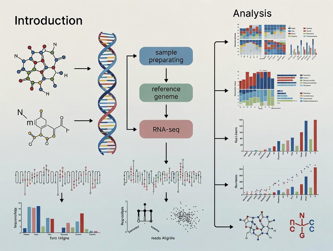
This guide provides researchers, scientists, and drug development professionals with a comprehensive roadmap for RNA-seq data analysis.
From Reads to Insights: A Scientist's Guide to Modern RNA-seq Data Analysis
Abstract
This guide provides researchers, scientists, and drug development professionals with a comprehensive roadmap for RNA-seq data analysis. It begins by establishing foundational concepts and experimental design principles (Intent 1). The core methodological section details the modern bioinformatics pipeline, from raw read processing to differential expression and pathway analysis (Intent 2). To ensure robust results, it addresses common troubleshooting scenarios, quality control pitfalls, and optimization strategies for diverse sample types (Intent 3). Finally, it covers critical validation techniques, discusses the comparative landscape of alternative transcriptomic methods, and explores translational applications (Intent 4). This structured approach equips wet-lab scientists with the knowledge to design, execute, and interpret RNA-seq experiments effectively for biomedical discovery.
RNA-seq Essentials: Laying the Groundwork for Successful Transcriptomics
What is RNA-seq? Core Principles and Key Applications in Biomedical Research
RNA sequencing (RNA-seq) is a high-throughput sequencing technology that provides a comprehensive, quantitative, and unbiased profile of the transcriptome—the complete set of RNA transcripts in a biological sample. This technical guide frames RNA-seq within the broader thesis of its data analysis pipeline, which is foundational for modern biomedical discovery. By converting RNA into a library of complementary DNA (cDNA) fragments with adapters, RNA-seq allows researchers to determine the presence and quantity of RNA, enabling insights into gene expression, alternative splicing, novel transcripts, and gene fusions.
Core Principles and Workflow
The fundamental principle of RNA-seq is the sequencing of cDNA derived from RNA. The standard workflow involves several critical steps:
Diagram Title: RNA-seq Core Experimental Workflow
Detailed Experimental Protocol: Standard Poly-A Selected mRNA-seq
Objective: To profile polyadenylated mRNA from eukaryotic cells.
Materials: See The Scientist's Toolkit below. Protocol:
- RNA Extraction & QC: Isolate total RNA using a guanidinium thiocyanate-phenol-chloroform method (e.g., TRIzol). Assess RNA integrity (RIN > 8.0) using an Agilent Bioanalyzer.
- Poly-A Selection: Use oligo(dT) magnetic beads to enrich for polyadenylated mRNA. Bind RNA to beads, wash away non-poly-A RNA (rRNA, tRNA), and elute purified mRNA.
- Fragmentation: Chemically or enzymatically fragment 10-1000 ng of purified mRNA to ~200-300 nucleotide fragments.
- cDNA Synthesis: Perform first-strand synthesis using reverse transcriptase and random hexamer primers. Synthesize second-strand cDNA with DNA Polymerase I/RNase H.
- Library Construction: End-repair cDNA fragments, add adenine (A) overhangs, and ligate platform-specific adapter sequences with barcodes (for multiplexing).
- Library Amplification & QC: Amplify the adapter-ligated library via PCR (typically 10-15 cycles). Validate library size distribution (~300-500 bp) and concentration via Bioanalyzer/qPCR.
- Sequencing: Pool multiplexed libraries and load onto a sequencer (e.g., Illumina NovaSeq). Perform paired-end sequencing (e.g., 2x150 bp) to a depth of 20-50 million reads per sample.
Key Applications in Biomedical Research
Differential Gene Expression (DGE) Analysis
This is the most common application, quantifying changes in gene expression levels between conditions (e.g., disease vs. healthy, treated vs. untreated).
Data Analysis Protocol for DGE:
- Quality Control: Use FastQC to assess read quality. Trim adapters and low-quality bases with Trimmomatic or Cutadapt.
- Alignment: Map reads to a reference genome using a splice-aware aligner (e.g., STAR, HISAT2).
- Quantification: Count reads aligning to genomic features (genes, exons) using featureCounts or HTSeq.
- Differential Analysis: Use statistical models in R/Bioconductor packages (DESeq2, edgeR, or limma-voom) to identify significantly differentially expressed genes (adjusted p-value < 0.05, |log2 fold change| > 1).
- Interpretation: Perform pathway and gene ontology enrichment analysis (using tools like clusterProfiler or GSEA) on the resulting gene list.
Table 1: Key Quantitative Outputs from a Typical DGE Study
| Metric | Typical Value/Range | Significance |
|---|---|---|
| Sequencing Depth | 20-50 million reads/sample | Balances cost and detection sensitivity. |
| Mapping Rate | 70-90% | Indicates quality of sample and reference. |
| Genes Detected | 10,000-15,000 (human) | Measures comprehensiveness of transcriptome capture. |
| Significant DEGs | Varies widely (100s to 1000s) | Depends on biological effect size and experimental design. |
| False Discovery Rate (FDR) | < 0.05 | Standard threshold for statistical significance. |
Detection of Alternative Splicing and Novel Isoforms
RNA-seq can identify different mRNA isoforms produced from a single gene locus.
Diagram Title: RNA-seq Identifies Alternative Splicing Isoforms
Single-Cell RNA-seq (scRNA-seq)
This application profiles transcriptomes of individual cells, uncovering cellular heterogeneity.
Protocol Highlights (10x Genomics Chromium Platform):
- Single-Cell Partitioning: A suspension of single cells is combined with gel beads containing barcoded oligo-dT primers within nanoliter-scale droplets.
- Reverse Transcription: Within each droplet, RNA from a single cell is reverse-transcribed, tagging all cDNA from that cell with a unique cell barcode. Each transcript also receives a unique molecular identifier (UMI).
- Library Prep: cDNA is pooled, amplified, and prepared for sequencing following a similar protocol to bulk RNA-seq but preserving cell-of-origin information via barcodes.
- Data Analysis: Tools like Cell Ranger align reads and generate a gene expression matrix (cells x genes). Downstream analysis with Seurat or Scanpy involves clustering, dimensionality reduction (UMAP/t-SNE), and marker identification.
Table 2: Key Applications and Their Research Impact
| Application | Primary Output | Impact in Drug Development & Research |
|---|---|---|
| Differential Expression | List of dysregulated genes/pathways | Identifies novel drug targets and biomarkers for disease. |
| Variant & Fusion Detection | Somatic mutations, gene fusions (e.g., EML4-ALK) | Enables precision oncology and targeted therapies. |
| scRNA-seq | Cell-type atlas, differentiation trajectories | Informs immunotherapy targets, understanding disease mechanisms at cellular resolution. |
| Immune Repertoire | B-cell & T-cell receptor diversity | Critical for vaccine development and autoimmune disease research. |
The Scientist's Toolkit: Essential Research Reagents & Materials
Table 3: Key Reagent Solutions for RNA-seq Library Preparation
| Item | Function | Example/Note |
|---|---|---|
| RNA Extraction Kit | Isolates high-integrity total RNA, free of genomic DNA and contaminants. | TRIzol, Qiagen RNeasy, or Monarch kits. Include DNase I treatment. |
| Poly-A Selection Beads | Enriches for messenger RNA by binding polyadenylated tails. | NEBNext Poly(A) mRNA Magnetic Beads, Dynabeads Oligo(dT). |
| RNA Fragmentation Buffer | Chemically breaks RNA into uniform fragments for optimal sequencing. | Often included in library prep kits (e.g., Illumina). |
| Reverse Transcriptase | Synthesizes first-strand cDNA from RNA template. | Must be high-fidelity and processive (e.g., SuperScript IV). |
| Second-Strand Synthesis Mix | Converts RNA:DNA hybrid to double-stranded cDNA. | Contains DNA Polymerase I, RNase H, and dNTPs. |
| Library Prep Kit | Contains enzymes and buffers for end-prep, A-tailing, adapter ligation, and PCR. | Illumina TruSeq, NEBNext Ultra II, Takara SMART-seq. |
| Size Selection Beads | Purifies and selects for correctly sized cDNA fragments. | SPRIselect or AMPure XP beads. |
| Unique Dual Indexes | Adapters with barcodes to multiplex multiple samples in one sequencing run. | Essential for sample pooling and demultiplexing. |
| Sequencing Platform | The instrument performing massively parallel sequencing. | Illumina NovaSeq/HiSeq, PacBio Sequel, Oxford Nanopore. |
This guide serves as a foundational chapter within a broader thesis on RNA-seq data analysis. The quality of biological conclusions drawn from an RNA-seq experiment is fundamentally dictated by decisions made during the experimental design phase. A poorly designed study cannot be salvaged by advanced bioinformatics. This section provides an in-depth technical guide to three pillars of robust design: achieving sufficient statistical power, determining replicate number, and implementing strategies to minimize technical and biological bias.
Core Principles of Experimental Design
Statistical Power and Replicate Number
Power is the probability of detecting a true difference in gene expression when one exists. Insufficient power leads to false negatives, wasting resources and missing biologically significant findings.
Key Determinants of Power:
- Effect Size: The minimum fold-change in expression you aim to detect (e.g., 1.5x, 2x). Smaller effect sizes require more replicates.
- Biological Variability: Inherent variation between individual organisms or cell cultures. Highly variable samples require more replicates.
- Technical Variability: Noise introduced during library preparation and sequencing. This can be reduced by technical replication but is best controlled by improving protocol consistency.
- Significance Threshold: The adjusted p-value (e.g., FDR < 0.05). More stringent thresholds reduce power.
- Sequencing Depth: The number of reads per sample. Beyond a certain point, adding replicates provides more power than increasing depth for differential expression analysis.
Recommendations from Current Literature: Recent studies and power analysis tools (e.g., Scotty, RNASeqPower, PROPER) emphasize that for model organisms or cell lines with controlled variability, biological replicates are non-negotiable. Technical replicates (multiple libraries from the same RNA sample) are not a substitute for biological replicates and are primarily useful for assessing technical noise.
Table 1: General Guideline for Biological Replicate Number (Animal/Cell Line Studies)
| Experimental Goal | Recommended Minimum Biological Replicates per Condition | Rationale |
|---|---|---|
| Pilot Study / Exploratory | 3 | Provides initial estimate of variance for full-study power calculation. |
| Differential Expression (Strong effect >2x) | 4-6 | Balances cost with reasonable power (e.g., >80%) for large changes. |
| Differential Expression (Subtle effect ≤1.5x) | 8-12 | Necessary to achieve sufficient power for detecting small fold-changes. |
| Time-course / Multi-condition | 4-6 per time point/condition | Increased complexity requires maintaining power across multiple comparisons. |
| Human patient cohorts (high variability) | 15-20+ | High biological variability necessitates large sample sizes. |
Protocol 2.1: Conducting an A Priori Power Analysis
- Estimate Parameters: Obtain an estimate of gene-wise dispersion/variance from a pilot study or public dataset from a similar system.
- Define Criteria: Set your target effect size (fold-change), significance threshold (e.g., FDR=0.05), and desired statistical power (e.g., 80%).
- Use a Power Tool: Utilize software to calculate the required number of replicates.
- Example using
PROPERin R:
- Example using
- Iterate: Run simulations across a range of replicate numbers (e.g., 3 to 12) to find the optimal cost-power balance for your study.
Avoiding and Controlling for Bias
Bias systematically distorts measurements away from the true value and must be minimized at every stage.
Major Sources of Bias:
- Sample Collection & Preparation: Time of day, handling stress, batch of reagents, RNA extraction method.
- Library Preparation: Technician, kit lot, library preparation date, RNA integrity (RIN) bias.
- Sequencing: Flow cell, lane, machine, and sequencing date effects.
Strategies to Mitigate Bias:
- Randomization: Randomly assign samples to treatment groups and processing batches.
- Blocking: Group similar experimental units together (e.g., littermates, cells from the same passage).
- Balancing: Ensure each technical batch contains an equal number of samples from each experimental condition. This turns a confounding batch effect into a blocked factor that can be modeled statistically.
Protocol 2.2: Implementing a Balanced Block Design
- List all samples with their biological group (e.g., Control, Treated) and blocking factor (e.g., litter, culture date).
- Assign a random number to each sample within each block.
- For library prep, assign the samples with the lowest random numbers from each biological group to Batch 1, the next set to Batch 2, etc., until all samples are assigned, ensuring balance across batches.
- Repeat this process for sequencing lane assignment, treating library prep batches as a new blocking factor if necessary.
- Record all metadata (group, block, batch, lane, technician, date) meticulously for downstream batch effect correction.
Diagram 1: Balanced Block Design Workflow (100 chars)
The Scientist's Toolkit: Key Research Reagent Solutions
Table 2: Essential Reagents & Kits for Robust RNA-seq Library Prep
| Item | Function & Importance for Reducing Bias |
|---|---|
| RNA Integrity Number (RIN) Analyzer (e.g., Bioanalyzer, TapeStation) | Critical. Quantifies RNA degradation. Using samples with similar, high RIN (>8 for most applications) prevents 3' bias. |
| Ribosomal RNA Depletion Kits (e.g., Ribo-zero, NEBNext rRNA Depletion) | Removes abundant ribosomal RNA, enriching for mRNA and non-coding RNA. Kit lot should be consistent or balanced. |
| mRNA Selection Beads (e.g., Poly(A) Magnetic Beads) | Isolates polyadenylated mRNA. Batch effects can arise; use a single, balanced lot per study. |
| Stranded Library Preparation Kit (e.g., NEBNext Ultra II, Illumina TruSeq Stranded) | Preserves strand orientation of RNA, crucial for accurate transcript annotation and avoiding antisense bias. |
| Unique Dual Index (UDI) Adapters | Allows unambiguous multiplexing of many samples, preventing sample index cross-talk (barcode hopping) bias. |
| High-Fidelity PCR Polymerase | Amplifies cDNA libraries with low error rates and minimal GC-bias during final library amplification. |
| Library Quantification Kit (e.g., qPCR-based) | Accurate molar quantification ensures balanced pooling of libraries, preventing sequencing depth bias. |
A Recommended Standard Workflow
The following workflow integrates the principles of power, replication, and bias avoidance.
Protocol 4.1: Integrated RNA-seq Experimental Pipeline
- Define Hypothesis & Power Analysis: Use pilot data or public data with a tool like
PROPERorScottyto determine the number of biological replicates required for adequate power. - Design with Balance & Randomization: Create a sample collection plan that records biological blocks. Design a laboratory workflow that balances experimental conditions across all technical batches (RNA extraction, library prep kits/lots/dates, sequencing lanes).
- Sample Collection & QC: Collect samples uniformly. Extract total RNA using a standardized, validated protocol. Assess RNA quality and quantity rigorously; exclude or note outliers.
- Library Preparation: Use a stranded library prep protocol. For all steps (rRNA depletion, fragmentation, cDNA synthesis, adapter ligation, PCR), keep meticulous records of reagent lots and technician. Use UDIs.
- Pooling & Sequencing: Quantify libraries precisely by qPCR. Pool in equimolar ratios. Sequence on a platform that provides sufficient depth (commonly 20-40 million reads per sample for standard differential expression).
- Metadata Compilation: Create a comprehensive sample sheet linking each sequenced file to all biological and technical metadata for downstream analysis.
Diagram 2: Integrated RNA-seq Design & Workflow (100 chars)
A meticulously planned RNA-seq experiment is the most critical step in generating reliable and biologically meaningful data. Investing resources in an appropriate number of randomized, balanced biological replicates—as determined by a power analysis—will yield far greater returns than maximizing sequencing depth alone. Simultaneously, rigorous recording and balancing of technical variables transform potential confounders into manageable factors. By adhering to these principles, researchers lay a solid foundation for the subsequent computational analysis chapters of this thesis, ensuring that the final interpretations reflect biology, not experimental artifact.
In RNA-seq data analysis, the initial quality assessment of raw sequencing data is a critical first step that determines the validity of all subsequent conclusions. This guide details the process from receiving raw FASTQ files to generating and interpreting quality control metrics with FastQC, framed within a comprehensive RNA-seq thesis. Ensuring data integrity at this stage is paramount for researchers, scientists, and drug development professionals who rely on accurate transcriptomic profiles for biomarker discovery and therapeutic target identification.
The Anatomy of a FASTQ File
A FASTQ file is the standard output format from high-throughput sequencers, containing both sequence data and per-base quality scores. Each record consists of four lines:
- Sequence Identifier: Begins with '@', containing instrument and flow cell data.
- Nucleotide Sequence.
- Separator Line: Begins with '+', sometimes followed by the identifier again.
- Quality Scores: Encoded as ASCII characters representing Phred quality scores (Q).
Table 1: Phred Quality Score (Q) Interpretation
| Phred Score (Q) | Probability of Incorrect Base Call | Base Call Accuracy | Typical ASCII Encoding (Sanger/Illumina 1.8+) |
|---|---|---|---|
| 10 | 1 in 10 | 90% | + |
| 20 | 1 in 100 | 99% | 5 |
| 30 | 1 in 1000 | 99.9% | ? |
| 40 | 1 in 10,000 | 99.99% | I |
FastQC: An In-Depth Methodology
FastQC is a ubiquitous tool that provides a modular set of analyses. The following protocol details its standard execution.
Experimental Protocol: Running FastQC
Materials:
- Computing Environment: Unix/Linux command line or Windows with appropriate shell.
- Software: Java Runtime Environment (JRE) version 8 or later.
- Input Data: One or more FASTQ files (gzip compression supported).
Procedure:
- Download and Install: Obtain FastQC from the Babraham Bioinformatics website. Unpack the archive.
- Make Executable: Ensure the script is executable.
- Run Analysis: Execute FastQC on your FASTQ file(s). Use the
-oflag to specify an output directory. - Review Output: FastQC generates an HTML report file (
sample_01_R1_fastqc.html) and a compressed data folder for each input file.
Interpreting Key FastQC Modules
Table 2: Core FastQC Module Results and Acceptable Thresholds for RNA-seq
| Module | Purpose | Ideal Result for RNA-seq | Potential Issue Indicated |
|---|---|---|---|
| Per Base Sequence Quality | Mean quality scores across all bases. | Q ≥ 28 for all bases. | Degradation at read ends suggests poor library prep or sequencing chemistry issues. |
| Per Sequence Quality Scores | Distribution of average read qualities. | Sharp peak in the high-quality region (e.g., Q>30). | Broad or bimodal distribution indicates a subset of low-quality reads. |
| Per Base Sequence Content | Proportion of each nucleotide (A,T,C,G) per cycle. | A/T and C/G lines parallel after ~5-10 bases. | Deviation indicates library contamination (e.g., adapter, primer) or overrepresented sequences. |
| Overrepresented Sequences | Lists sequences appearing >0.1% of total. | None listed. | Presence of adapters, primers, or ribosomal RNA (common in RNA-seq) indicates enrichment bias. |
| Adapter Content | Quantifies adapter sequence contamination. | Near 0% across all bases. | Rising curve indicates significant adapter contamination, necessitating trimming. |
Note: RNA-seq data often legitimately fails "Per Base Sequence Content" and "Overrepresented Sequences" due to non-random start sites of cDNA fragments and expected ribosomal RNA reads, respectively.
The Scientist's Toolkit: RNA-seq QC Essential Materials
Table 3: Research Reagent Solutions for RNA-seq Library Preparation and QC
| Item | Function in RNA-seq Workflow |
|---|---|
| Poly(A) Selection Beads (e.g., oligo-dT beads) | Enriches for messenger RNA (mRNA) by binding polyadenylated tails. Critical for eukaryotic transcriptomes. |
| Ribosomal Depletion Kits (e.g., Ribo-Zero) | Removes abundant ribosomal RNA (rRNA) from total RNA, essential for prokaryotic or degraded samples. |
| RNA Fragmentation Buffer (Metal cations) | Chemically or enzymatically fragments RNA to optimal size for sequencing library construction. |
| Reverse Transcriptase (e.g., SuperScript IV) | Synthesizes first-strand cDNA from RNA template. High processivity and fidelity are crucial. |
| Double-Stranded DNA (dsDNA) High-Sensitivity Assay Kit (e.g., Qubit) | Accurately quantifies dilute library concentrations prior to sequencing. |
| Library Quantification Kit for qPCR (e.g., KAPA Biosystems) | Quantifies the concentration of amplifiable library fragments with adapters for precise sequencing loading. |
| High-Sensitivity DNA Chip (e.g., Agilent Bioanalyzer/TapeStation) | Assesses library fragment size distribution and detects adapter dimer contamination. |
Visualizing the RNA-seq Quality Control Workflow
Diagram 1: FastQC Analysis and Decision Workflow (84 chars)
Diagram 2: FASTQ Quality Score Encoding Scheme (73 chars)
Rigorous quality assessment using FastQC on raw FASTQ files establishes the foundation for robust and reproducible RNA-seq analysis. Understanding the metrics and their implications within the biological context of RNA sequencing allows researchers to make informed decisions about data remediation and to proceed with confidence into alignment, quantification, and differential expression analysis, ultimately supporting valid scientific and clinical conclusions.
Within the broader thesis of RNA-seq data analysis, the library preparation step is the critical foundation upon which all subsequent computational and biological interpretations are built. The choices made here—regarding RNA input, strandedness, and scale—fundamentally determine the scope, accuracy, and applicability of the generated data. This guide provides an in-depth technical comparison of core strategies to inform experimental design for researchers and drug development professionals.
Input RNA: mRNA vs. Total RNA
The decision between poly(A)-selected mRNA and ribosomal RNA (rRNA)-depleted total RNA defines the transcriptomic landscape accessible to sequencing.
Poly(A) Selection (mRNA-seq): Enriches for transcripts with a polyadenylated tail, primarily capturing protein-coding mRNAs and some long non-coding RNAs (lncRNAs). It is efficient and clean but will miss non-polyadenylated RNA species (e.g., histone mRNAs, some lncRNAs, and bacterial RNAs).
rRNA Depletion (Total RNA-seq): Removes ribosomal RNA sequences (which constitute >80% of total RNA) via probe hybridization, preserving both polyA+ and polyA- transcripts. This enables the study of non-coding RNAs, pre-mRNAs, viral RNAs, and transcripts with degraded poly(A) tails, often crucial in clinical or degraded samples.
Quantitative Comparison of RNA Input Types
| Feature | Poly(A) Selection (mRNA-seq) | rRNA Depletion (Total RNA-seq) |
|---|---|---|
| Primary Target | Polyadenylated RNA (mRNA, some lncRNAs) | All RNA except rRNA |
| Typical Input | 10 ng – 1 µg total RNA (high quality, RIN >8) | 10 ng – 1 µg total RNA (more tolerant of moderate degradation) |
| Efficiency | High enrichment; minimal rRNA reads (<5%) | Variable; residual rRNA reads typically 5-30% |
| Coverage | Coding transcriptome, 3'-biased with standard protocols | Whole transcriptome, including ncRNA, pre-mRNA, retained introns |
| Cost & Protocol | Generally lower cost; simpler protocol | Higher cost; more complex hybridization/wash steps |
| Ideal Applications | Differential gene expression in healthy tissue/cell lines | Gene expression in non-polyA transcripts, degraded FFPE samples, pathogen detection, novel transcript discovery |
Strandedness: Preserving Transcript Orientation
Standard, non-stranded protocols lose information about which original DNA strand was transcribed. Stranded library preparation retains this orientation, which is critical for:
- Accurately quantifying overlapping genes on opposite strands.
- Identifying antisense transcription and regulatory non-coding RNAs.
- Correctly annotating novel transcripts.
Key Methodologies for Stranded Libraries:
- dUTP/Second-Strand Marking: The most common method. During cDNA synthesis, dTTP is replaced with dUTP in the second strand. The dUTP-containing strand is subsequently enzymatically degraded (using Uracil-Specific Excision Reagent, USER) before PCR amplification, ensuring only the first strand is amplified. This yields libraries where the sequenced read 1 corresponds to the antisense of the original RNA.
- Adaptor Ligation to RNA: Adaptors are ligated directly to the RNA molecule before reverse transcription, physically marking the original strand. This method can be more robust for degraded samples.
- Template-Switching (e.g., SMART): Used prominently in single-cell and low-input protocols. The reverse transcriptase enzyme adds non-templated nucleotides upon reaching the 5' end of the RNA, allowing a template-switching oligo (TSO) to bind and extend, creating a full-length cDNA copy with known, common adaptor sequences on both ends.
Diagram 1: Stranded library prep via dUTP/second-strand marking.
Single-Cell RNA-Seq (scRNA-seq) Considerations
scRNA-seq introduces extreme input material constraints (picograms of RNA) and the need to capture cell-specific barcodes, demanding specialized library preparation.
Core Workflow Paradigms:
- Droplet-Based (e.g., 10x Genomics): Cells are partitioned into nanoliter droplets with gel beads carrying unique barcodes and poly(T) primers. Reverse transcription occurs inside each droplet, tagging all cDNA from a single cell with the same cell barcode. Libraries are prepared from the pooled, barcoded cDNA.
- Plate-Based (Smart-seq2): Cells are sorted into individual wells. Full-length cDNA is generated using a template-switching protocol, followed by tagmentation or PCR-based library construction. This offers superior sensitivity and coverage per cell but at lower throughput.
Critical Protocol Steps for scRNA-seq:
- Cell Viability and Quality: >90% viability is crucial to minimize background from ambient RNA.
- Reverse Transcription & Barcoding: High-efficiency RT is paramount. Cell and Unique Molecular Identifier (UMI) barcodes are incorporated during this step to track transcript origin and mitigate PCR duplication bias.
- cDNA Amplification: Requires a highly uniform and efficient PCR to amplify the femtogram amounts of cDNA without introducing severe bias.
- Library Construction: Often involves tagmentation (fragmentation and adapter insertion in one step by a transposase like Tn5) for efficiency from small cDNA inputs.
Diagram 2: High-throughput droplet-based scRNA-seq workflow.
The Scientist's Toolkit: Key Research Reagent Solutions
| Reagent / Kit | Primary Function |
|---|---|
| Poly(A) Magnetic Beads | Bind polyadenylated tails for mRNA purification and selection from total RNA. |
| Ribo-depletion Probes | Species-specific oligonucleotides that hybridize to rRNA for its removal from total RNA samples. |
| Template Switching Oligo (TSO) | Enables full-length cDNA capture during reverse transcription by providing a known sequence for primer extension. Critical for Smart-seq2 and many low-input protocols. |
| UMI Adapters | Oligonucleotides containing unique molecular identifiers to label individual RNA molecules pre-amplification, enabling accurate digital counting. |
| Tn5 Transposase | Engineered transposase that simultaneously fragments double-stranded DNA and ligates sequencing adapters. Essential for fast, efficient library prep in NGS. |
| USER Enzyme | Uracil-Specific Excision Reagent. Cleaves cDNA strands containing dUTP, enabling strand-specific library generation. |
| Single-Cell Barcoded Beads | Gel beads pre-loaded with millions of unique barcode combinations for massively parallel cell and transcript tagging in droplet-based systems. |
| SPRI Beads | Magnetic beads for size selection and clean-up of nucleic acids during library preparation (e.g., removing primers, adapter dimers, selecting fragment sizes). |
This whitepaper serves as a technical guide within the broader thesis on RNA-seq data analysis for scientific research. The central challenge in contemporary genomics is aligning specific biological questions with the correct analytical workflows. Three cornerstone applications—quantitative gene expression, full-length isoform detection, and gene fusion discovery—exemplify this need. Each goal demands distinct experimental designs, computational tools, and interpretation frameworks. This document provides an in-depth examination of these three pillars, equipping researchers and drug development professionals with the protocols and rationale to execute robust, goal-oriented RNA-seq studies.
Core Analytical Goals and Technology Alignment
The choice of RNA-seq library preparation and sequencing technology is paramount and must be dictated by the primary research objective. The following table summarizes the key alignment.
Table 1: Alignment of Research Goals to RNA-seq Methodologies
| Primary Goal | Recommended Library Prep | Optimal Sequencing | Critical QC Metric | Key Advantage |
|---|---|---|---|---|
| Gene Expression | Poly-A selected, stranded | Short-read (75-150 bp PE), High depth (>30M reads/sample) | rRNA depletion, Library Complexity | Cost-effective, High accuracy for abundance |
| Isoform Detection | Poly-A selected, stranded | Long-read (PacBio HiFi, ONT cDNA), Moderate depth | Read Length N50, cDNA integrity | Resolves full-length transcripts, Direct isoform identification |
| Fusion Discovery | rRNA-depived (total RNA), stranded | Short-read (100-150 bp PE), Very High depth (>50M reads/sample) | Broad expression range, Low adapter contamination | Detects fusions from non-polyadenylated RNA |
Detailed Experimental Protocols
Protocol for Stranded mRNA-seq (Gene Expression & Isoform Detection)
Principle: Enrich for polyadenylated RNA and preserve strand orientation.
- RNA QC: Verify RNA Integrity Number (RIN) > 8.5 (Agilent Bioanalyzer).
- Poly-A Selection: Use oligo-dT magnetic beads to bind mRNA.
- Fragmentation & cDNA Synthesis: Fragment purified mRNA chemically, followed by first-strand cDNA synthesis with random hexamers and Actinomycin D. Perform second-strand synthesis with dUTP incorporation for strand marking.
- Library Construction: End-repair, A-tailing, and adapter ligation. Perform UDG digestion to degrade the second strand (dUTP-containing), ensuring strand specificity.
- PCR Enrichment: Amplify with indexed primers for 10-15 cycles.
- QC & Pooling: Quantify by qPCR, check fragment size (TapeStation), and equimolar pool.
- Sequencing: Sequence on Illumina platform for 75-150 bp paired-end.
Protocol for Fusion Discovery (Total RNA-seq)
Principle: Capture all RNA species, including non-polyadenylated transcripts where fusion partners may reside.
- RNA QC: Verify RIN > 7.0.
- rRNA Depletion: Use ribo-depletion kits (e.g., Ribo-Zero) to remove cytoplasmic and mitochondrial rRNA.
- Fragmentation & cDNA Synthesis: Fragment enriched RNA and synthesize cDNA (stranded protocol as in 3.1).
- Library Construction & Sequencing: Follow steps 4-7 from Protocol 3.1, aiming for higher sequencing depth.
Protocol for Long-Read Isoform Sequencing (Iso-Seq)
Principle: Generate full-length cDNA reads without fragmentation.
- Full-Length cDNA Synthesis: Use SMARTer or similar technology with template-switching oligos to generate full-length, reverse-transcribed cDNA.
- cDNA Size Selection: Use BluePippin or Circulomics to select cDNAs > 1 kb.
- PCR Barcoding: Amplify size-selected cDNA with barcoded primers.
- SMRTbell or Nanopore Library Prep: For PacBio: blunt-ligate cDNA to SMRTbell adapters. For Oxford Nanopore: ligate sequencing adapters to cDNA.
- Sequencing: Sequence on PacBio Sequel II/Revio (HiFi mode) or ONT PromethION.
Computational Workflows and Key Tools
The analysis pipelines diverge significantly after raw data generation. The following diagram illustrates the logical relationships and decision points in a multi-goal RNA-seq analysis strategy.
Diagram Title: RNA-seq Analysis Workflow Decision Tree
The Scientist's Toolkit: Key Research Reagent Solutions
Table 2: Essential Reagents and Kits for RNA-seq Applications
| Item | Function | Example Product(s) |
|---|---|---|
| RNA Integrity Assay | Assesses RNA degradation; critical for library success. | Agilent RNA 6000 Nano Kit (Bioanalyzer) |
| Poly-A Selection Beads | Enriches for eukaryotic mRNA by binding poly-A tail. | NEBNext Poly(A) mRNA Magnetic Isolation Module |
| Ribo-depletion Kits | Removes ribosomal RNA from total RNA for fusion/RNA species analysis. | Illumina Ribo-Zero Plus, QIAseq FastSelect |
| Stranded cDNA Synthesis Kit | Creates strand-specific cDNA libraries, preserving transcript orientation. | NEBNext Ultra II Directional RNA Library Kit |
| Long-read cDNA Prep Kit | Generates full-length, amplified cDNA for isoform sequencing. | PacBio Iso-Seq Express Kit, ONT cDNA-PCR Seq Kit |
| UMI Adapters | Introduces Unique Molecular Identifiers to correct for PCR duplicates. | Illumina TruSeq UDI Adapters, SMARTer UMI oligos |
| High-Fidelity PCR Mix | Amplifies library fragments with minimal bias and errors. | KAPA HiFi HotStart ReadyMix, Q5 Hot Start DNA Polymerase |
| Magnetic Size Selection Beads | Performs clean-up and size selection of DNA fragments. | SPRISelect Beads (Beckman Coulter) |
| Library Quantification Kit | Accurate qPCR-based quantification prior to sequencing. | KAPA Library Quantification Kit |
| Sequencing Control | Spiked-in RNA/DNA controls for run and quantification monitoring. | External RNA Controls Consortium (ERCC) spikes |
Advanced Analysis and Pathway Context
Gene fusions and isoform switches often converge on core oncogenic signaling pathways. Identifying these downstream effects is crucial for interpreting functional impact.
Diagram Title: Signaling Pathways Impacted by Fusions and Isoforms
Table 3: Typical Output Metrics and Benchmarks for RNA-seq Applications
| Analysis Type | Typical Sequencing Depth | Key Output Metric | Expected Resolution/Benchmark | Common Downstream Analysis |
|---|---|---|---|---|
| Differential Gene Expression | 20-50 million reads/sample | Gene-level counts (e.g., TPM, FPKM) | Detects 2-fold change for 90% power in most genes | DESeq2, edgeR, limma-voom; GSEA, ORA |
| Differential Isoform Usage | 50-100 million reads/sample | Isoform proportion (Percent Spliced In - PSI) | Detects ΔPSI > 0.1-0.2 with confidence | SUPPA2, DEXSeq, rMATS; switch analysis |
| Fusion Gene Discovery | 50-150 million reads/sample | # of spanning/split reads per candidate | >5 spanning & >1 split read = high confidence | Arriba, STAR-Fusion; reciprocal validation |
| Full-Length Isoform Sequencing | 2-5 million HiFi reads/sample | # of unique, high-confidence isoforms | 10,000-30,000 isoforms per mammalian cell line | Iso-seq3, FLAIR; novel isoform detection |
The RNA-seq Pipeline Decoded: A Step-by-Step Walkthrough for Scientists
Within the broader thesis of establishing a robust RNA-seq data analysis pipeline for biomedical research, the pre-processing of raw sequencing reads is the critical first computational step. This phase transforms raw, instrument-generated data (FASTQ files) into clean, analysis-ready sequences. The accuracy of all downstream interpretations—differential gene expression, variant calling, and pathway analysis—is fundamentally contingent upon the rigor applied here. For drug development professionals, inconsistencies or artifacts introduced at this stage can lead to erroneous biological conclusions, impacting target identification and validation. This guide details the technical principles and current best practices for this essential cleaning process.
Core Concepts and Necessity
Sequencing instruments, particularly those using Illumina's Sequencing By Synthesis (SBS) technology, produce reads that contain not only the biological sequence of interest but also technical sequences (adapters) and low-quality bases. Adapters are short oligonucleotide sequences necessary for the sequencing process itself but must be identified and removed as they do not originate from the sample. Furthermore, sequencing quality typically degrades along the read length. Failure to address these issues leads to misalignment, reduced mapping rates, and biases in quantitative analysis.
Detailed Methodologies and Protocols
Adapter Trimming
Adapter contamination arises when the DNA/RNA fragment length is shorter than the read length, causing the sequencer to read into the adapter sequence on the opposite strand.
Protocol: Adapter Trimming with cutadapt (Current Best Practice)
- Input: Raw FASTQ files (R1 and R2 for paired-end).
- Tool:
cutadapt(v4.0+). It supports linked adapters for paired-end data and handles dual indexing correctly. - Command Example:
-a: Adapter sequence for the 3' end of read 1.-A: Adapter sequence for the 3' end of read 2.--minimum-length: Discard reads shorter than this after trimming.--max-n: Discard reads containing any ambiguous bases (N).--pair-filter=any: If either read in a pair is discarded, discard both.
Quality Trimming and Filtering
Quality scores (Phred scores) are per-base estimates of error probability. Low-quality bases hinder accurate alignment.
Protocol: Quality-based Trimming with fastp
- Tool:
fastpis a comprehensive all-in-one pre-processing tool known for speed. - Command Example:
--detect_adapter_for_pe: Automatically detects and trims adapters.--qualified_quality_phred: Base quality threshold (Q20).--unqualified_percent_limit: Allows up to 40% of bases to be below Q20 before discarding the read.--length_required: Minimum read length post-trimming.--json/--html: Generates detailed quality control reports.
Table 1: Impact of Pre-processing on Typical Human RNA-seq Data
| Metric | Raw Reads | After Adapter & Quality Trimming | Common Target Range |
|---|---|---|---|
| Total Reads (Paired-end) | 100% | 90-95% | >85% retention |
| Reads with Adapter Content | 5-40%* | <0.5% | Minimized |
| Average Read Quality (Phred Score) | 30-35 | 35-37 | Q30+ |
| % Bases ≥ Q30 | 85-92% | >95% | Maximized |
| Downstream Impact: | |||
| Alignment Rate | — | +3-10% | Typically >90% |
| PCR Duplicate Rate | — | May increase | Monitor |
Varies significantly with library prep and fragment size. *Cleaning removes more low-quality/artifact reads, potentially increasing the relative proportion of PCR duplicates, making duplicate marking more critical later.
Table 2: Comparison of Popular Pre-processing Tools (2024)
| Tool | Primary Strength | Adapter Handling | Quality Control | Speed | Best For |
|---|---|---|---|---|---|
cutadapt |
Precision, flexibility | Excellent (explicit sequences) | Basic trimming | Moderate | Standardized, protocol-aware workflows |
fastp |
All-in-one, speed | Excellent (auto-detection) | Comprehensive, per-read sliding window | Very Fast | Fast turnaround, integrated QC |
Trimmomatic |
Robustness, PE-aware | Good (pre-defined files) | Sliding window & leading/trailing | Fast | Bulk RNA-seq, established pipelines |
fastp + cutadapt |
Maximum control | Optimal | Comprehensive | Moderate | Critical applications requiring utmost precision |
The Scientist's Toolkit: Research Reagent Solutions
Table 3: Essential Reagents and Materials for Library Preparation Impacting Pre-processing
| Item | Function in Library Prep | Impact on Raw Reads & Pre-processing |
|---|---|---|
| Poly(A) Selection Beads | Enriches for mRNA by binding poly-A tails. | Reduces ribosomal RNA reads, affecting complexity. Incomplete removal leads to rRNA contamination detectable in QC. |
| RNA Fragmentation Reagents | Enzymatically or chemically fragments RNA to optimal size. | Determines insert size. Over-fragmentation leads to short inserts and high adapter content, increasing trimming burden. |
| RT & PCR Enzymes | Reverse transcription and library amplification. | Enzyme fidelity influences error rates. PCR over-amplification creates duplicate reads, identified post-alignment. |
| Size Selection Beads (SPRI) | Selects cDNA fragments within a target size range. | Critical for controlling insert size distribution. Poor size selection results in variable adapter content and uneven coverage. |
| Dual-Indexed Adapters | Unique molecular identifiers for sample multiplexing. | Allows simultaneous processing of multiple samples. Index hopping, though rare, must be checked for in downstream steps. |
| Library Quantification Kits | Accurate measurement of library concentration (qPCR-based). | Ensures balanced sequencing depth across samples, preventing low-coverage outliers in the final dataset. |
Visualized Workflows
Title: RNA-seq Read Pre-processing and QC Workflow
Title: Adapter Contamination and Trimming Schematic
Genome Alignment and Spliced Read Mapping with STAR or HISAT2
Within the broader thesis of RNA-seq data analysis for biomedical research, the accurate alignment of sequencing reads to a reference genome is a critical foundational step. This process is complicated by the biological phenomenon of RNA splicing, where introns are removed from pre-mRNA transcripts. Standard DNA read aligners fail to account for these discontinuities. Thus, specialized spliced aligners like STAR and HISAT2 are essential. Their performance directly impacts downstream analyses such as differential gene expression, novel isoform discovery, and fusion gene detection—key pursuits for researchers and drug development professionals aiming to understand disease mechanisms and identify therapeutic targets.
STAR (Spliced Transcripts Alignment to a Reference)
STAR utilizes a novel sequential maximum mappable seed (MMP) search in two stages. It first seeds alignments using Maximal Mappable Prefix (MMP) matches, which are contiguous sequences exactly matching the reference. It then performs detailed stitching and scoring of these seeds to construct full alignments, allowing for large gaps indicative of introns. Its speed derives from uncompressed suffix array-based genome indexing.
HISAT2 (Hierarchical Indexing for Spliced Alignment of Transcripts 2)
HISAT2 employs a hierarchical graph FM-index (GFM) that integrates a global genome index with numerous local indexes for common splice sites and exonic combinations. This architecture allows it to rapidly traverse potential splice junctions. It uses the Bowtie2 algorithm as its core for extending alignments from seeds found via the hierarchical index.
Table 1: Quantitative Comparison of STAR and HISAT2
| Feature | STAR | HISAT2 |
|---|---|---|
| Primary Algorithm | Maximal Mappable Prefix (MMP) search | Hierarchical Graph FM-index (GFM) |
| Index Type | Suffix Array | Burrows-Wheeler Transform (BWT) / FM-index |
| Typical RAM Usage | High (~32 GB for human) | Moderate (~10 GB for human) |
| Speed | Very Fast | Fast |
| Splice Junction Discovery | De novo (annotation-free) possible | Strongly benefits from annotation |
| Alignment Output | Primary & multiple mappings detailed | Configurable focus on primary mappings |
| Best Suited For | Large datasets, novel junction detection, speed-critical pipelines | Resource-constrained environments, annotated genomes |
Detailed Experimental Protocols
Protocol 1: Genome Indexing with STAR
Objective: Generate a genome index for subsequent alignment.
- Gather Input Files: Reference genome FASTA file (
GRCh38.primary_assembly.genome.fa) and gene annotation GTF file (gencode.v44.annotation.gtf). - Command:
--runThreadN: Number of CPU threads.--sjdbOverhang: Read length minus 1. Critical for junction database construction.
- Output: A directory containing the binary genome index.
Protocol 2: RNA-seq Read Alignment with STAR
Objective: Map paired-end FASTQ reads to the indexed genome.
- Input: Index directory, paired-end FASTQ files (
sample_R1.fastq.gz,sample_R2.fastq.gz). - Command:
--outSAMtype: Directly outputs sorted BAM.--quantMode GeneCounts: Generates read counts per gene.
Protocol 3: Genome Indexing with HISAT2
Objective: Build a hierarchical graph-based index.
- Input: Reference genome FASTA file.
- Command:
- Optionally, incorporate known splice sites:
--ssand--exonoptions using extracted splice site data from a GTF.
- Optionally, incorporate known splice sites:
Protocol 4: RNA-seq Read Alignment with HISAT2
Objective: Map reads using the HISAT2 index.
- Input: HISAT2 index, paired-end FASTQ files.
- Command:
Visualized Workflows
Title: STAR Alignment and Quantification Workflow
Title: HISAT2 with StringTie Transcript Assembly Pipeline
The Scientist's Toolkit: Research Reagent Solutions
Table 2: Essential Reagents and Tools for Spliced Alignment Experiments
| Item | Function in Experiment |
|---|---|
| High-Quality Total RNA Extraction Kit (e.g., Qiagen RNeasy, TRIzol) | Isolates intact, degradation-free RNA for library prep, crucial for accurate junction mapping. |
| Strand-Specific RNA-seq Library Prep Kit (e.g., Illumina TruSeq Stranded mRNA) | Preserves transcript orientation information, critical for accurate gene annotation and antisense transcription analysis. |
| RNA Integrity Number (RIN) Analyzer (e.g., Agilent Bioanalyzer) | Quantifies RNA degradation; high RIN (>8) is essential for full-length transcript representation. |
| Ultra-Pure DNase/RNase-Free Water | Prevents nucleic acid degradation and enzyme inhibition during library preparation. |
| PCR Enzyme for Library Amplification (e.g., KAPA HiFi HotStart) | Provides high-fidelity amplification with minimal bias, ensuring equitable representation of all transcripts. |
| Size Selection Beads (e.g., SPRIselect) | Cleans up enzymatic reactions and selects for optimally sized cDNA fragments prior to sequencing. |
| Sequencing Control Spikes (e.g., ERCC RNA Spike-In Mix) | Adds known quantities of synthetic RNAs to assess technical sensitivity, dynamic range, and alignment accuracy. |
| Alignment Software (STAR or HISAT2) | The core computational tool performing the spliced alignment algorithm. |
| High-Performance Computing (HPC) Resources | Essential for memory-intensive indexing (STAR) and processing large sequencing datasets in parallel. |
The quantification of mapped sequencing reads into gene- or transcript-level counts is a critical step in the RNA-seq data analysis pipeline. Following alignment, the digital gene expression matrix serves as the fundamental data structure for all downstream statistical analyses, including differential expression, pathway analysis, and biomarker discovery. For scientists and drug development professionals, the choice of quantification tool directly impacts the robustness, reproducibility, and biological validity of their conclusions. This guide provides an in-depth technical comparison of two established, alignment-based quantification tools: FeatureCounts (part of the Subread package) and HTSeq. We focus on their methodologies, practical implementation, and suitability for different experimental designs prevalent in biomedical research.
Core Tool Comparison: Methodology and Performance
The following table summarizes the key quantitative and methodological characteristics of FeatureCounts and HTSeq, based on recent benchmark studies.
Table 1: Technical Comparison of FeatureCounts and HTSeq
| Feature | FeatureCounts (Subread) | HTSeq (htseq-count) |
|---|---|---|
| Primary Method | Alignment-based, exon-to-gene summarization. | Alignment-based, union-exon model with overlap resolution. |
| Speed | Very fast; utilizes chromosome indexing and built-in multi-threading. | Slower; processes alignments sequentially in a single thread. |
| Memory Efficiency | High. | Moderate. |
| Strandedness Handling | Comprehensive support for stranded protocols (0,1,2). | Full support for stranded (yes, reverse, no) and non-stranded assays. |
| Multi-mapping Reads | Can assign to primary alignment or distribute fractionally (via --fraction). |
Default behavior is to ignore ambiguous reads (--nonunique none). Options: none, all, fraction. |
| Overlap Resolution | Prioritizes longest overlap; can use meta-features. | Strict hierarchical rule: gene > exon > intergenic. |
| Annotation Input | GTF/GFF format, SAF (Simplified Annotation Format). | GTF format. |
| Output Format | Simple tab-delimited count matrix. | Simple tab-delimited count vector per sample. |
| Best Suited For | High-throughput studies, large sample numbers, time-sensitive projects. | Studies requiring precise, conservative counting based on strict genomic overlap rules. |
Detailed Experimental Protocols
Protocol for Quantification with FeatureCounts
Objective: To generate a gene-level count matrix from aligned BAM files for a stranded, paired-end RNA-seq experiment.
Research Reagent Solutions & Essential Materials:
- Aligned Reads: Sequence Alignment/Map (BAM) files from a splice-aware aligner (e.g., STAR, HISAT2). Sorted by genomic coordinate is required.
- Genome Annotation: A reference genome annotation file in Gene Transfer Format (GTF).
- Software: Subread package (v2.0.0+) installed.
- Computing Environment: Linux/Unix server or high-performance computing cluster with sufficient memory (≥8 GB recommended).
Step-by-Step Method:
- Prepare the Environment: Ensure Subread is in your
$PATH. Organize BAM files and the GTF annotation file in your working directory. - Basic Command for Single Sample: Run
featureCountson one BAM file to test parameters.-T 8: Use 8 CPU threads.-s 2: Strand-specific protocol, reverse stranded (e.g., Illumina TruSeq).-a: Path to the GTF file.-o: Output file name.
- Batch Processing for Multiple Samples: Use a shell loop or job array.
- Generate Consolidated Matrix: The primary output file (
sample1.counts.txt) contains a summary section and the counts. The count columns from individual sample outputs must be merged into a single matrix using a script (e.g., in R or Python) for downstream analysis.
Protocol for Quantification with HTSeq (htseq-count)
Objective: To generate gene-level counts using strict overlap resolution for a non-stranded, single-end RNA-seq experiment.
Research Reagent Solutions & Essential Materials:
- Aligned Reads: Sorted BAM files. Must be name-sorted if paired-end.
- Genome Annotation: A GTF file with identical chromosome/contig naming as the BAM files.
- Software: HTSeq Python package (v0.13.0+) installed.
- Computing Environment: Python environment. Lower memory requirement but longer run time.
Step-by-Step Method:
- Prepare Input Files: Ensure BAM files are sorted. For paired-end, they must be sorted by read name (
samtools sort -n). - Basic Command for Single Sample:
-f bam: Input format is BAM.-s no: Assay is non-stranded.-r pos: BAM file is sorted by genomic position (usenamefor name-sorted paired-end).--additional-attr: Adds the gene_name attribute to the output.
- Process Multiple Samples: Similar loop structure as above.
- Post-Processing: HTSeq outputs five special counters at the end of the file (e.g.,
__no_feature,__ambiguous). These lines must be removed before merging individual count files into a matrix. This is crucial for accurate differential expression analysis.
Visualized Workflows and Logical Relationships
Title: RNA-seq Quantification Workflow: FeatureCounts vs HTSeq
Title: Read Assignment Logic: FeatureCounts vs HTSeq
This whitepaper serves as a technical guide within a broader thesis on RNA-seq data analysis. Differential expression (DE) analysis is a cornerstone of transcriptomics, enabling researchers to identify genes whose expression changes significantly between experimental conditions. This guide details the core statistical models of three predominant tools: DESeq2, edgeR, and limma-voom, providing methodologies for their application in drug development and basic research.
Core Statistical Models and Assumptions
Each package employs a distinct model to handle count data's mean-variance relationship.
DESeq2: Uses a negative binomial (NB) distribution. Dispersion is estimated by a shrinkage approach that borrows information across genes, improving stability for experiments with few replicates. It tests using the Wald test or Likelihood Ratio Test (LRT).
edgeR: Also uses an NB model. It offers multiple dispersion estimation methods: common, trended, and tagwise. Quasi-likelihood (QL) methods can be used for increased robustness against outlier counts. Testing is via exact tests or QL F-tests.
limma-voom: Transforms count data using the voom function, which estimates the mean-variance relationship to generate precision weights. These weighted log-counts are then analyzed using limma's empirical Bayes moderated t-test framework, designed for continuous microarray-like data.
Quantitative Comparison of Key Features
Table 1: Core characteristics of DESeq2, edgeR, and limma-voom.
| Feature | DESeq2 | edgeR | limma-voom |
|---|---|---|---|
| Primary Distribution | Negative Binomial | Negative Binomial | Gaussian (after voom) |
| Dispersion Estimation | Shrinkage towards trend | Common, Trended, Tagwise / QL | Mean-variance trend used for weights |
| Statistical Test | Wald test / LRT | Exact test / QL F-test | Moderated t-test (eBayes) |
| Handling of Small Replicates | Strong via dispersion shrinkage | Good, enhanced with QL | Good with precise weighting |
| Speed | Moderate | Fast | Very Fast (post-voom) |
| Optimal Use Case | Experiments with limited replicates, complex designs | Flexible, offers both classic & QL pipelines | Large-scale experiments, multiple contrasts |
Table 2: Typical input requirements and output metrics.
| Parameter | Typical Requirement / Value |
|---|---|
| Minimum Recommended Replicates | 3 per condition (statistical rigor increases with more) |
| Recommended Sequencing Depth | 10-30 million reads per library (mammalian genomes) |
| Key Output Metric | Log2 Fold Change (LFC), Adjusted p-value (FDR) |
| Common FDR Threshold | < 0.05 or < 0.01 |
| Typical Normalization Method | DESeq2: Median of ratios; edgeR: TMM; limma-voom: TMM then voom |
Experimental Protocols
Protocol 1: Standard RNA-seq Workflow for DE Analysis
- Library Preparation & Sequencing: Generate strand-specific, poly-A enriched RNA-seq libraries. Sequence on an Illumina platform to a minimum depth of 20 million paired-end 150bp reads per sample.
- Quality Control: Assess raw read quality using FastQC. Trim adapters and low-quality bases with Trimmomatic or Cutadapt.
- Alignment: Map cleaned reads to a reference genome using a splice-aware aligner (e.g., STAR, HISAT2). For Homo sapiens, use GRCh38.
- Quantification: Generate gene-level read counts using featureCounts or HTSeq-count, using a comprehensive annotation file (e.g., GENCODE).
- DE Analysis (Example: DESeq2):
a. Construct a
DESeqDataSetobject from the count matrix and sample metadata. b. RunDESeq(): This performs estimation of size factors, dispersion estimation, and model fitting. c. Extract results using theresults()function, specifying the contrast of interest. Apply independent filtering and log2 fold change shrinkage (lfcShrink) as appropriate. - Interpretation: Filter significant genes (FDR < 0.05, |LFC| > 1). Perform functional enrichment analysis (GO, KEGG).
Protocol 2: Validation by qRT-PCR
- Primer Design: Design SYBR Green or TaqMan assays for 5-10 significant DE genes and 2-3 stable reference genes (e.g., GAPDH, ACTB).
- cDNA Synthesis: Reverse transcribe 1µg of the same input RNA using a high-capacity cDNA reverse transcription kit.
- qPCR Reaction: Perform reactions in triplicate 10µL reactions on a 384-well plate using a master mix. Use a standard two-step thermal cycling protocol.
- Analysis: Calculate ∆Ct values relative to reference genes, then ∆∆Ct between conditions. Correlate log2 fold changes with RNA-seq results.
Visualized Workflows and Relationships
Title: RNA-seq Differential Expression Analysis Core Workflow
Title: Tool Selection Guide Based on Experimental Design
The Scientist's Toolkit: Research Reagent Solutions
Table 3: Essential reagents and materials for RNA-seq-based DE analysis.
| Item | Function in Workflow | Example Product / Kit |
|---|---|---|
| RNA Isolation Kit | High-quality total RNA extraction from cells/tissues, preserving mRNA integrity. | Qiagen RNeasy Kit, Zymo Research Quick-RNA Kit |
| Poly-A Selection Beads | Enrichment of messenger RNA from total RNA by binding polyadenylated tails. | NEBNext Poly(A) mRNA Magnetic Isolation Module |
| Library Prep Kit | Converts mRNA to a sequenceable library (fragmentation, cDNA synthesis, adapter ligation, indexing). | Illumina Stranded mRNA Prep, NEBNext Ultra II RNA Library Prep |
| RNA Quantification Assay | Accurate measurement of RNA concentration and assessment of purity (260/280 ratio). | Qubit RNA BR Assay, Agilent Bioanalyzer RNA Nano Kit |
| qRT-PCR Master Mix | For validation of DE results via quantitative reverse transcription PCR. | SYBR Green (Bio-Rad, Thermo Fisher), TaqMan Gene Expression Master Mix |
| RNase Inhibitor | Protects RNA samples from degradation during handling and storage. | Recombinant RNase Inhibitor (Takara, Lucigen) |
This guide, part of a broader thesis on RNA-seq data analysis, details essential methods for interpreting differential gene expression results. Following statistical identification of significant genes, researchers must translate lists into biological understanding. Gene Ontology (GO) term enrichment and pathway analysis via Gene Set Enrichment Analysis (GSEA) and the Kyoto Encyclopedia of Genes and Genomes (KEGG) are foundational techniques.
Core Concepts and Methodologies
Gene Ontology (GO) Enrichment Analysis
GO provides a controlled vocabulary describing gene functions across three domains: Biological Process (BP), Molecular Function (MF), and Cellular Component (CC). Enrichment analysis identifies GO terms over-represented in a query gene list compared to a background set (e.g., all expressed genes).
Detailed Protocol: Hypergeometric Test for GO Enrichment
- Input Preparation: Generate a list of differentially expressed genes (DEGs) (e.g., padj < 0.05, |log2FC| > 1). Define a background list (typically all genes detected in the RNA-seq experiment).
- Term Association: Map all genes in both lists to GO terms using a current annotation database (e.g., org.Hs.eg.db for human, from Bioconductor).
- Contingency Table Construction: For each GO term, create a 2x2 table:
- a: Number of DEGs annotated to the term.
- b: Number of background genes annotated to the term, minus a.
- c: Number of DEGs not annotated to the term.
- d: Number of background genes not annotated to the term, minus c.
- Statistical Testing: Apply the hypergeometric test (or Fisher's exact test) to calculate a p-value for the over-representation of the term in the DEG list.
- Multiple Testing Correction: Apply a correction method (e.g., Benjamini-Hochberg) to control the False Discovery Rate (FDR). Terms with FDR < 0.05 are considered significantly enriched.
- Visualization: Plot results as bar charts, dot plots, or directed acyclic graphs.
Gene Set Enrichment Analysis (GSEA)
GSEA evaluates whether a priori defined gene sets show statistically significant, concordant differences between two biological states. It uses all genes from an expression dataset ranked by their association with a phenotype.
Detailed Protocol: Pre-ranked GSEA
- Gene Ranking: Rank all genes from the RNA-seq experiment by a metric of differential expression (e.g., signal-to-noise ratio, log2 fold change). The ranking is typically from the most up-regulated in phenotype A to the most down-regulated.
- Gene Set Database: Select a collection of gene sets (e.g., GO, KEGG, Hallmark, or custom sets).
- Enrichment Score (ES) Calculation: For a given gene set S, walk down the ranked list. Increase a running-sum statistic when a gene in S is encountered, decrease it when a gene not in S is encountered. The magnitude of the increment is based on the gene's correlation with the phenotype. The ES is the maximum deviation from zero of the running sum.
- Significance Assessment: Permute the phenotype labels (or gene labels for pre-ranked) 1000+ times to generate a null distribution of ES. The nominal p-value is derived from this distribution.
- FDR Correction: Normalize ES for gene set size (NES). Calculate the FDR by comparing the proportion of false positives from permuted data to observed results.
- Leading Edge Analysis: Identify the subset of genes within the gene set that contribute most to the enrichment signal at the point where the ES is calculated.
KEGG Pathway Analysis
KEGG maps molecular datasets to curated graphical diagrams of biological pathways. Enrichment analysis can be performed similarly to GO (over-representation analysis) or via GSEA.
Detailed Protocol: KEGG Over-Representation Analysis
- Pathway Mapping: Convert gene identifiers to KEGG Orthology (KO) identifiers using tools like
clusterProfiler(R) or KEGG Mapper. - Statistical Test: Perform a hypergeometric test for each KEGG pathway, comparing the number of DEGs mapped to a pathway versus the expected number from the background.
- FDR Correction: Adjust p-values for multiple testing.
- Pathway Visualization: Use KEGG Mapper's "Color" tool to visually project gene expression data (e.g., log2FC) onto pathway maps.
Table 1: Comparison of Downstream Interpretation Methods
| Feature | GO Enrichment | GSEA | KEGG ORA |
|---|---|---|---|
| Core Principle | Over-representation of terms in a significant gene list. | Rank-based enrichment across an entire expression profile. | Over-representation of genes in curated pathways. |
| Input | A threshold-derived list of DEGs. | A full, ranked gene list from an experiment. | A threshold-derived list of DEGs. |
| Key Strength | Simple, intuitive for focused gene lists. | Captures subtle, coordinated expression changes; no arbitrary threshold. | Direct biological context via well-defined pathway maps. |
| Key Limitation | Highly dependent on significance threshold. | Computationally intensive; requires careful parameter selection. | Pathway coverage is not exhaustive; bias toward well-annotated processes. |
| Primary Output | List of enriched GO terms with p/FDR. | List of enriched gene sets with NES, FDR, leading edge. | List of enriched pathways with p/FDR; colored pathway diagrams. |
| Best Applied When | You have a clear, high-confidence DEG list. | You have subtle, genome-wide expression shifts or want to compare phenotypes holistically. | You need mechanistic, pathway-level hypotheses for validation. |
Table 2: Common Statistical Output Metrics
| Metric | Formula/Description | Typical Threshold | ||
|---|---|---|---|---|
| Fold Change (FC) | 2^(log2FC) |
>2 or <0.5 (for log2FC >1 or <-1) | ||
| Adjusted P-value (padj) | Benjamini-Hochberg FDR correction. | < 0.05 | ||
| Enrichment Score (ES) | Max deviation of running-sum statistic in GSEA. | N/A (see NES) | ||
| Normalized ES (NES) | ES normalized for gene set size. | NES | > 1.5 | |
| False Discovery Rate (FDR) | Estimated probability that a gene set is a false positive. | < 0.25 (GSEA standard) or <0.05 | ||
| Gene Ratio | (# genes in list & term) / (# genes in list) | Higher ratio indicates stronger enrichment. |
Visual Workflows and Pathways
Downstream Analysis Workflow
GO Enrichment Analysis Protocol
Example KEGG Pathway: MAPK Signaling
The Scientist's Toolkit
Table 3: Essential Research Reagents & Tools for Enrichment Analysis
| Item | Function & Description |
|---|---|
| RNA-seq Alignment & Quantification Tools (STAR, Salmon, Kallisto) | Map sequencing reads to a reference genome/transcriptome and estimate gene/transcript abundance. Essential for generating input data. |
| Differential Expression Software (DESeq2, edgeR, limma-voom) | Statistical R/Bioconductor packages to identify genes differentially expressed between conditions. Produces the ranked gene list. |
| Annotation Databases (org.Xx.eg.db, Ensembl, MSigDB) | Provide mappings between gene identifiers (e.g., Ensembl ID) and functional terms (GO, KEGG pathways, Hallmark sets). |
| Enrichment Analysis Suites (clusterProfiler, g:Profiler, Enrichr, fgsea) | R packages or web tools that perform hypergeometric tests and GSEA, integrating current annotation databases. |
| Pathway Visualization Tools (KEGG Mapper, Pathview, Cytoscape) | Project expression data onto pathway diagrams (KEGG) or create custom network visualizations of results. |
| Multiple Testing Correction Algorithms (Benjamini-Hochberg, Bonferroni) | Statistical methods to control false positives when testing thousands of hypotheses (GO terms/pathways) simultaneously. |
Navigating RNA-seq Challenges: QC, Batch Effects, and Advanced Normalization
Within the broader thesis of RNA-seq data analysis, sample quality is the foundational determinant of experimental success. The integrity of extracted RNA dictates the fidelity of downstream sequencing, alignment, and differential expression analysis. This guide provides a technical deep-dive into diagnosing RNA degradation via the RNA Integrity Number (RIN) and other QC metrics, and outlines robust protocols for remediation and prevention of sample failure.
Quantitative Assessment of RNA Quality
The following tables summarize key quantitative metrics and their interpretation.
Table 1: RIN Score Interpretation and Implications for RNA-seq
| RIN Score | Interpretation | Recommended for RNA-seq? | Primary Degradation Indicator |
|---|---|---|---|
| 10.0 - 9.0 | Excellent Integrity | Yes, ideal | Sharp 18S/28S ribosomal peaks. |
| 8.9 - 7.0 | Good Integrity | Yes, suitable | Slight reduction in 28S:18S ratio. |
| 6.9 - 5.0 | Moderate Degradation | Caution; may require protocol adjustment | Broadened ribosomal peaks, increased lower molecular weight smear. |
| 4.9 - 3.0 | Significant Degradation | Problematic; requires remediation or specialized kits | Loss of 28S peak, prominent smear. |
| < 3.0 | Severe Degradation | No, not suitable | No ribosomal peaks, extensive degradation. |
Table 2: Complementary QC Metrics for RNA Sample Assessment
| Metric | Tool/Method | Optimal Range | Indication of Failure |
|---|---|---|---|
| DV200 (%) | Fragment Analyzer, Bioanalyzer | >70% for FFPE; >85% for fresh/frozen | High proportion of fragments <200 nucleotides. |
| 28S/18S Ratio | Bioanalyzer, TapeStation | ~2.0 for mammalian total RNA | Ratio <1.5 suggests degradation. |
| Concentration (ng/µL) | Fluorometry (Qubit) | Dependent on input requirements | Inaccuracies from spectrophotometry (A260/A280) due to contaminants. |
| A260/A280 | Spectrophotometry (NanoDrop) | 1.8 - 2.0 | Deviation indicates protein or solvent contamination. |
| A260/A230 | Spectrophotometry (NanoDrop) | 2.0 - 2.2 | Low values suggest guanidine salts or phenol carryover. |
Experimental Protocols for QC and Remediation
Protocol 3.1: Accurate RNA Integrity Assessment Using a Bioanalyzer
Objective: To determine the RIN score and electrophoretic profile of total RNA samples. Materials: Agilent Bioanalyzer 2100, RNA Nano or Pico Kit, thermal cycler, RNase-free tubes and tips. Procedure:
- Gel-Dye Mix Preparation: Thaw RNA dye concentrate and filter cartridge. Pipette 550 µL of RNA gel matrix into a spin filter, centrifuge at 1500 ± 50 g for 10 minutes at room temperature. Add 65 µL of filtered gel to a RNA dye concentrate vial, vortex, and centrifuge.
- Chip Priming: Load 9 µL of gel-dye mix into the well marked "G". Place the chip in the priming station, close the lid, and press the plunger until held by the clip. Wait exactly 30 seconds, then release the clip. Wait 5 seconds, then slowly pull back the plunger to its home position.
- Sample Loading: Pipette 9 µL of conditioning solution into the well marked "CS". Load 5 µL of RNA marker into each sample well (ø11) and ladder well (ø1). Load 1 µL of each RNA sample (1-50 ng/µL) into subsequent sample wells.
- Chip Run and Analysis: Vortex the chip for 1 minute at 2400 rpm. Place chip in the Bioanalyzer and run the "RNA Nano" assay. The software automatically calculates RIN and 28S/18S ratio.
Protocol 3.2: RNA Clean-up and Remediation Using Solid-Phase Reversible Immobilization (SPRI) Beads
Objective: To remove contaminants (salts, solvents, proteins) and recover intact RNA from partially degraded samples. Materials: RNase-free SPRI beads (e.g., AMPure XP RNA Clean Beads), 80% ethanol, RNase-free water, magnetic stand, low-retention tips. Procedure:
- Binding: Mix RNA sample (up to 50 µL) with 1.8X volume of room-temperature SPRI beads. Vortex thoroughly and incubate for 5 minutes at room temperature.
- Washing: Place tube on a magnetic stand for 5 minutes until supernatant clears. Carefully remove and discard supernatant. With tube on magnet, add 200 µL of freshly prepared 80% ethanol. Incubate 30 seconds, then remove ethanol. Repeat wash once. Air-dry pellet for 2-5 minutes (do not over-dry).
- Elution: Remove tube from magnet. Resuspend bead pellet in 15-30 µL of RNase-free water. Incubate for 2 minutes. Place back on magnet for 5 minutes. Transfer the clean RNA supernatant to a new tube. Quantify using Qubit.
Protocol 3.3: rRNA Depletion for Partially Degraded Samples (RIN 4-6)
Objective: To enable RNA-seq of degraded samples by targeting the remaining intact mRNA. Materials: Commercial rRNA depletion kit (e.g., Illumina Ribo-Zero Plus), thermal cycler, magnetic stand. Procedure:
- Hybridization: Combine 5-1000 ng of total RNA (in ≤10 µL) with 5 µL of rRNA removal solution. Add RNase-free water to 15 µL. Mix and incubate in a thermal cycler at 68°C for 5 minutes, then 37°C for 10 minutes.
- rRNA Capture: Add 15 µL of RNase-free water and 20 µL of magnetic probe removal beads to the reaction. Mix well and incubate at 37°C for 15 minutes.
- Bead Separation: Place tube on magnetic stand for 5 minutes. Carefully transfer the supernatant (~50 µL) containing rRNA-depleted RNA to a new tube. Proceed immediately to library preparation.
Visualizations
Title: RNA Sample QC and Remediation Workflow
Title: Key Pathways Leading to RNA Degradation
The Scientist's Toolkit: Essential Research Reagents & Materials
Table 3: Key Reagent Solutions for RNA Quality Control and Remediation
| Item | Function | Critical Notes |
|---|---|---|
| RNase Inhibitors (e.g., Recombinant RNasin) | Inactivates RNases during extraction and handling. | Essential for all steps post-homogenization. Add fresh to buffers. |
| RNA-specific SPRI Beads (e.g., AMPure XP RNA) | Selective binding of RNA for clean-up and size selection. | More reproducible than ethanol precipitation. Optimize bead:sample ratio. |
| Fluorometric RNA Assay Dyes (Qubit RNA HS/BR) | Accurate quantification of RNA concentration. | Binds specifically to RNA, unaffected by common contaminants. |
| Capillary Electrophoresis Chips (Bioanalyzer RNA Nano/Pico) | Assess integrity (RIN) and size distribution (DV200). | Pico assay for limited or dilute samples (<5 ng/µL). |
| Ribosomal RNA Depletion Kits (Ribo-Zero Plus, AnyDeplete) | Remove abundant rRNA to enrich mRNA in degraded samples. | Critical for FFPE or low-RIN samples. Choose based on sample type. |
| RNA Stabilization Reagents (RNAlater, PAXgene) | Penetrate tissue to inhibit RNase activity immediately upon collection. | Soak small tissue pieces completely. |
| DNase I, RNase-free | Remove genomic DNA contamination post-extraction. | Perform on-column or in-solution; include Mg2+ buffer. |
| Nuclease-free Water and Buffers | Solvent for resuspension and reaction setup. | Certified free of RNases. Do not use DEPC-treated water post-extraction. |
Identifying and Correcting for Technical Batch Effects (ComBat, RUV)
Within the comprehensive framework of an RNA-seq data analysis thesis, the management of non-biological variation is a foundational step. Technical batch effects—systematic errors introduced by factors such as processing date, sequencing lane, or operator—can confound biological signals and lead to spurious conclusions. This whitepaper provides an in-depth technical guide to two prominent methodologies for identifying and correcting these effects: ComBat and Remove Unwanted Variation (RUV). Mastery of these tools is essential for researchers, scientists, and drug development professionals aiming to derive robust, reproducible insights from high-throughput sequencing data.
Core Methodologies
ComBat (Combining Batches)
ComBat uses an empirical Bayes framework to adjust for batch effects while preserving biological variability. It models the data as a combination of biological covariates of interest and known batch variables.
Detailed Protocol:
- Input Data Preparation: Start with a normalized gene expression matrix (genes x samples). Ensure batch identifiers (e.g., Batch1, Batch2) and any desired biological covariates (e.g., disease status) are defined.
- Model Specification: Fit a linear model for each gene g:
Y_gi = α_g + Xβ_g + γ_bi + δ_bi * ε_giwhere:Y_giis the expression for gene g in sample i.α_gis the overall gene expression level.Xβ_grepresents the design matrix for biological covariates.γ_biandδ_biare the additive and multiplicative batch effects for batch b.ε_giis the error term.
- Empirical Bayes Estimation: Pool information across genes to estimate the batch effect parameters (
γ_bi,δ_bi), shrinking them towards the overall mean. This step stabilizes estimates for small sample sizes. - Adjustment: Apply the estimated parameters to adjust the data:
Y_gi* = (Y_gi - γ_bi) / δ_bi - Output: The corrected gene expression matrix.
Remove Unwanted Variation (RUV)
RUV methods correct for batch effects using control genes or replicate samples that are not expected to exhibit biological variation of interest (e.g., housekeeping genes, spike-in controls, or technical replicates).
Common Variations and Protocols:
RUVg (Using Control Genes):
- Identify a set of k negative control genes assumed to be invariant across biological conditions (e.g., ERCC spike-ins or empirically defined least variable genes).
- Perform factor analysis (e.g., SVD) on the control genes alone to estimate the k factors of unwanted variation (
W). - Fit a regression model including
Was covariates alongside biological variables of interest to the full dataset. - Obtain the residuals as the corrected expression values.
RUVs (Using Replicate Samples):
- Identify sets of samples that are technical replicates (identical biological condition processed in different batches).
- Within each set of replicates, calculate the differences from the replicate mean to estimate the unwanted variation.
- Pool these estimates across all replicate sets to form the unwanted factors (
W). - Proceed with regression and residual calculation as in RUVg.
RUVr (Using Residuals):
- Perform a first-pass regression of the expression data on the biological covariates of interest.
- The residuals from this model contain both unwanted variation and noise.
- Estimate the factors of unwanted variation (
W) from these residuals via factor analysis. - Refit the model including
Wto obtain the final corrected data.
Comparative Analysis of Methods
Table 1: Quantitative Comparison of Batch Effect Correction Methods
| Feature | ComBat | RUVg | RUVs | RUVr |
|---|---|---|---|---|
| Core Input Requirement | Known batch labels | List of control genes | Replicate sample structure | None (uses residuals) |
| Underlying Model | Empirical Bayes linear model | Factor analysis (regression on latent factors) | Factor analysis (regression on latent factors) | Factor analysis (regression on latent factors) |
| Preservation of Biological Signal | High (when covariates specified) | Moderate-High (dependent on control gene quality) | High (good for designed experiments) | Variable (risk of removing biological signal) |
| Handling of Unknown Batch Effects | No | Yes | Yes | Yes |
| Typical Runtime | Fast | Moderate (depends on k) | Moderate (depends on k) | Slower (two-step regression) |
| Key Advantage | Powerful adjustment for known batches with small-n stabilization. | Corrects for both known and unknown factors. | Leverages experimental design for accurate estimation. | Does not require controls or replicates. |
| Primary Limitation | Requires explicit batch labels; may over-correct. | Quality critically depends on control gene selection. | Requires replicate samples in design. | Highest risk of removing biological variance. |
Table 2: Common Performance Metrics from Batch Effect Correction Studies*
| Metric | Pre-Correction (Typical Range) | Post-ComBat (Typical Range) | Post-RUV (Typical Range) | Ideal Goal |
|---|---|---|---|---|
| PVCA (Percent Variance Explained by Batch) | 15-40% | <5% | <10% | Minimize |
| Silhouette Score (Batch)* | >0.3 (batch clusters) | <0.1 | <0.2 | Minimize |
| Silhouette Score (Biology)* | Variable, often low | >0.3 | >0.25 | Maximize |
| Differential Expression (DE) Precision (F1-Score) | 0.6-0.75 | 0.8-0.95 | 0.75-0.9 | Maximize |
| *PVCA = Principal Variance Component Analysis. *Silhouette Score: Higher values indicate tighter clustering. |
Table data synthesized from recent benchmarking literature (2022-2024).
Visualization of Workflows and Relationships
Title: ComBat and RUV Correction Workflow Comparison
Title: The Confounding Problem of Batch Effects
The Scientist's Toolkit: Research Reagent Solutions
Table 3: Essential Materials and Tools for Batch Effect Management
| Item | Category | Function in Batch Effect Correction |
|---|---|---|
| ERCC Spike-In Mix | Control Reagent | Exogenous RNA controls added to each sample at known concentrations. Used in RUVg as ideal negative controls to estimate technical variation. |
| UMI (Unique Molecular Identifier) Adapters | Sequencing Reagent | Enables accurate quantification of absolute molecule counts, reducing amplification and sequencing depth batch effects at the library level. |
| Validated Housekeeping Gene Panels | Assay Reagent | Sets of endogenous genes empirically shown to be stable. Can serve as control genes for RUVg when spike-ins are unavailable. |
| Commercial RNA Reference Standards | Reference Material | Well-characterized RNA samples (e.g., from cell lines) processed across batches to monitor and quantify technical variability. |
| sva (Surrogate Variable Analysis) R Package | Software Tool | Provides functions for ComBat and for estimating surrogate variables for unknown batch effects. Industry standard for known-batch correction. |
| ruv R Package | Software Tool | Implements the RUVg, RUVs, and RUVr algorithms. Essential for factor-based correction using controls or replicates. |
| limma R Package | Software Tool | Provides the removeBatchEffect function (simple linear adjustment) and integrates seamlessly with ruv for differential analysis post-correction. |
| Single-Cell RNA-seq Platform Controls | Control Reagent | For single-cell studies, cell hashing reagents or ambient RNA removal kits (e.g., SoupX) mitigate batch effects specific to droplet-based platforms. |
In RNA-seq data analysis, normalization is a critical preprocessing step that enables accurate comparison of gene expression levels across samples and experiments. This technical guide, framed within a broader thesis on RNA-seq data analysis for scientific research, explores and contrasts traditional count normalization methods (TPM, FPKM, RPKM) with variance-stabilizing transformations (VSTs). These strategies address the inherent challenges of sequencing data, including library size differences, gene length biases, and mean-variance relationships. For researchers, scientists, and drug development professionals, selecting the appropriate normalization method is foundational for downstream analyses such as differential expression, clustering, and biomarker discovery.
Core Normalization Methods: Principles and Calculations
Traditional Count-Based Normalizations
These methods generate normalized expression estimates by adjusting raw read counts for technical artifacts.
- RPKM (Reads Per Kilobase per Million mapped reads): Developed for single-end RNA-seq. Normalizes for sequencing depth and gene length.
- Calculation:
RPKM = (read counts * 10^9) / (gene length in kb * total mapped reads)
- Calculation:
- FPKM (Fragments Per Kilobase per Million mapped reads): The paired-end counterpart to RPKM, where a fragment (two reads) corresponds to a single cDNA molecule.
- Calculation:
FPKM = (fragment counts * 10^9) / (gene length in kb * total mapped fragments)
- Calculation:
- TPM (Transcripts Per Million): A successor to RPKM/FPKM that first normalizes for gene length, then for sequencing depth. This method produces a proportional measure where the sum of all TPM values in a sample is 1 million, allowing for more direct sample-to-sample comparison.
- Calculation:
Rate = read counts / gene length in kbPerMillionScalingFactor = sum(all Rates in sample) / 1,000,000TPM = Rate / PerMillionScalingFactor
- Calculation:
Variance-Stabilizing Transformations (VST)
VSTs, such as those implemented in tools like DESeq2, address a fundamental property of count data: the variance increases with the mean. These transformations remove this dependence, ensuring that genes with high expression do not dominate the variance in analyses like PCA. The vst or rlog functions in DESeq2 use a fitted dispersion-mean relationship to apply a transformation that yields homoskedastic (approximately constant variance) data across the dynamic range. This is particularly crucial for linear modeling and distance-based exploratory analyses.
The table below summarizes the key characteristics, applications, and limitations of each normalization strategy.
Table 1: Comparison of RNA-seq Normalization Strategies
| Feature | RPKM/FPKM | TPM | Variance-Stabilizing Transformation (VST) |
|---|---|---|---|
| Primary Purpose | Within-sample gene expression comparison. | Within- and between-sample comparison. | Stabilize variance across mean expression for downstream stats. |
| Corrects For | Sequencing depth, gene length. | Gene length, then sequencing depth. | Mean-variance relationship, library size. |
| Output Scale | Unbounded continuous. Sum varies per sample. | Sum is 1 million for all samples. | Log2-like continuous. Variance is approximately constant. |
| Between-Sample Comparison | Problematic due to inconsistent per-sample sums. | Valid, as values represent relative abundance. | Excellent, as required for comparative statistical tests. |
| Optimal Use Case | Historical or legacy data; qualitative visualization. | Relative expression profiling, e.g., comparing isoform ratios. | Differential expression analysis, PCA, clustering, machine learning. |
| Key Limitation | Not suitable for differential expression between samples. | Does not model count distribution or variance. | Requires a fitted model (e.g., via DESeq2); less intuitive units. |
Experimental Protocols for Key Methodologies
Protocol 1: Generating TPM Values from Raw Counts
- Input Data: A matrix of raw gene/transcript read counts and a corresponding vector of gene lengths (in nucleotides).
- Calculate Reads per Kilobase: For each gene in each sample, divide the raw count by the gene length (in kilobases).
Rate = count / (length/1000). - Sum All Rates: For each sample, calculate the sum of all
Ratevalues. - Compute Per-Million Scaling Factor: Divide the sum from Step 3 by 1,000,000.
- Calculate TPM: For each gene, divide its
Rate(from Step 2) by the sample-specific scaling factor (from Step 4).TPM = Rate / ScalingFactor.
Protocol 2: Applying a Variance-Stabilizing Transformation with DESeq2
- Construct DESeqDataSet: Create a
DESeqDataSetobject from a matrix of integer counts, sample information, and a design formula (e.g.,~ condition). - Estimate Size Factors: Run
DESeq(dds, fitType="parametric")to estimate size factors (for library size normalization) and gene-wise dispersions. - Apply VST: Use the
vst()orrlog()function on theDESeqDataSetobject. Thevstis faster and recommended for larger datasets.vsd <- vst(dds, blind=FALSE). - Extract Matrix: Retrieve the transformed matrix for downstream analysis:
transformed_matrix <- assay(vsd).
Visual Workflows and Logical Relationships
Title: RNA-seq Normalization Method Decision Workflow
Title: TPM Calculation Data Flow
The Scientist's Toolkit: Research Reagent Solutions
Table 2: Essential Resources for RNA-seq Normalization and Analysis
| Item / Solution | Provider / Example | Function in Analysis |
|---|---|---|
| RNA Extraction Kit | Qiagen RNeasy, Zymo Quick-RNA | Isolates high-quality, intact total RNA from biological samples. |
| Poly-A Selection Beads | NEBNext Poly(A) mRNA Magnetic | Enriches for messenger RNA by binding polyadenylated tails, removing rRNA and other RNA. |
| cDNA Synthesis & Library Prep Kit | Illumina TruSeq Stranded mRNA | Converts RNA to cDNA, adds adapters, and amplifies to create sequencer-compatible libraries. |
| High-Performance Computing Cluster | Local HPC, Cloud (AWS, Google) | Provides the computational power required for aligning reads and running normalization pipelines. |
| Alignment Software | STAR, HISAT2 | Maps sequenced reads (FASTQ) to a reference genome to generate count data (BAM/SAM). |
| Quantification Software | featureCounts, HTSeq, Salmon | Summarizes aligned reads per genomic feature (gene/transcript) to produce the raw count matrix. |
| Analysis Suite (R/Bioconductor) | DESeq2, edgeR, limma-voom | Performs statistical normalization (e.g., VST), modeling, and differential expression testing. |
| Interactive Analysis Environment | RStudio, Jupyter Notebook | Provides an integrated environment for scripting, visualization, and documenting the analysis. |
Handling Low-Expression Genes and Addressing Dropouts in Single-Cell RNA-seq
Within the broader thesis on RNA-seq data analysis, single-cell RNA sequencing (scRNA-seq) presents unique challenges distinct from bulk sequencing. The limited starting material per cell leads to two intertwined technical artifacts: the prevalence of genes with very low or zero counts (low-expression genes) and stochastic failure to detect expressed genes, known as "dropouts." These issues confound biological variation with technical noise, complicating downstream analysis such as differential expression, trajectory inference, and cell type identification. This technical guide provides an in-depth examination of the sources, impacts, and computational/experimental strategies for mitigating these critical challenges.
The fundamental cause of dropouts is the low capture efficiency of transcripts during library preparation. While bulk RNA-seq may sequence 70-90% of transcripts, scRNA-seq protocols typically capture only 10-20%. This results in a significant fraction of truly expressed genes having zero counts. Low-expression genes are inherently susceptible to this, but even moderately expressed genes can be affected.
Table 1: Typical Capture Efficiencies and Dropout Rates by scRNA-seq Platform
| Platform | Typical Capture Efficiency | Estimated Dropout Rate for a Gene with 10 Transcripts/Cell | Key Factors Influencing Dropout |
|---|---|---|---|
| Smart-seq2 | 20-30% | ~40% | Full-length, plate-based, higher sensitivity. |
| 10x Genomics (3') | 10-15% | ~70-80% | Droplet-based, 3' biased, high throughput. |
| Drop-seq | 5-10% | >85% | Early droplet method, lower efficiency. |
| inDrops | 10-15% | ~70-80% | Similar to 10x, different chemistry. |
| CEL-seq2 | 15-25% | ~50-60% | Unique molecular identifiers (UMIs), 3' biased. |
Table 2: Impact of Sequencing Depth on Gene Detection
| Mean Reads per Cell | Median Genes Detected per Cell (Human) | Approx. % of Biological Transcripts Sampled |
|---|---|---|
| 20,000 | 1,000 - 2,000 | <10% |
| 50,000 | 2,500 - 4,000 | 15-20% |
| 100,000 | 4,000 - 7,000 | 25-30% |
| 500,000 | 8,000 - 12,000 | 40-50% |
Computational Imputation and Correction Methods
Imputation aims to distinguish technical zeros from true biological absence and recover likely expression values. Each method has distinct assumptions and trade-offs between noise reduction and over-smoothing.
Detailed Protocol: Benchmarking Imputation Methods
- Data Preparation: Start with a raw UMI count matrix (cells x genes). Filter low-quality cells (high mitochondrial %, low gene counts) and genes expressed in <10 cells.
- Create Ground Truth (Simulation): Use a synthetic benchmark like
splatterR package. Simulate a scRNA-seq dataset with known dropouts using a negative binomial model, introducing zeros based on a logistic function of gene mean expression (e.g.,dropout.midparameter set to 3). - Apply Imputation: Run several key algorithms on the simulated data with observed dropouts.
- MAGIC: (
magicR/python).magic_func <- magic(raw_matrix, solver='approximate', t=6). The diffusion timetis critical. - SAVER: (
saverR).saver_output <- saver(raw_matrix, ncores=4). Returns posterior mean estimates. - scImpute: (
scImputeR).scimpute(count_path, infile="csv", outfile="csv", type="count", drop_thre=0.5). Identifies and imputes only "likely dropouts." - ALRA: (
ALRAR).alra_output <- alra(raw_matrix)[[3]]. Based on k-rank approximation.
- MAGIC: (
- Evaluation Metrics: Calculate on held-out, non-zero-inflated data or known truth.
- Root Mean Square Error (RMSE) between imputed and true normalized values.
- Pearson correlation of gene-gene relationships pre- and post-imputation.
- Improvement in clustering resolution (Silhouette score).
- Recovery of known rare cell type markers.
Table 3: Comparison of Major Imputation Algorithms
| Method | Core Principle | Strengths | Weaknesses | Best For |
|---|---|---|---|---|
| MAGIC | Data diffusion via Markov affinity graph. | Powerful denoising, reveals gene-gene relationships. | Can over-smooth, alters data structure. | Pathway analysis, continuous dynamics. |
| SAVER | Bayesian shrinkage towards a gene-specific prior. | Provides uncertainty estimates, conservative. | Computationally intensive for large datasets. | Recovering true expression magnitude. |
| scImpute | Model-based, imputes only likely dropouts. | Preserves true zeros, avoids global smoothing. | Relies on cluster identification step. | Datasets with clear subpopulations. |
| ALRA | Adaptive low-rank approximation (SVD). | Fast, deterministic, preserves sparsity of zeros. | Assumes low-rank structure of data. | Large-scale datasets (e.g., 10x Genomics). |
| DCA | Deep count autoencoder with ZINB model. | Models count distribution and dropouts explicitly. | Complex training, potential for overfitting. | Modeling complex, non-linear noise. |
Experimental and Protocol-Based Solutions
Computational correction has limits; experimental improvements are foundational.
Detailed Protocol: Multiplexed scRNA-seq with Sample Pooling (Cell Hashing) This protocol uses antibody-derived tags to multiplex samples, increasing cell throughput and allowing for deeper sequencing per cell without cost increase.
- Labeling Cells with Hashing Antibodies: For each of 8 separate cell suspensions (e.g., different conditions), label with a unique TotalSeq-B or TotalSeq-C anti-species Hashtag antibody (e.g., BioLegend) for 30 minutes on ice. Use 0.5-1µg antibody per 100,000 cells in 50µL buffer.
- Pooling: Wash each sample twice with PBS + 0.04% BSA. Combine all 8 labeled samples into a single tube. The cells are now distinguishable by their hashtag oligonucleotide.
- Library Preparation: Process the pooled sample through your standard scRNA-seq pipeline (e.g., 10x Genomics Chromium). This generates two libraries: the GENE EXPRESSION library (cDNA) and the HASHTOG library (antibody-derived tags).
- Demultiplexing: After sequencing, use tools like
CITE-seq-CountorCellRanger(v7+) to generate hashtag count matrices. Apply a deconvolution algorithm (HTODemuxin Seurat,hashedDropsin DropletUtils) to assign each cell barcode to its sample of origin based on the hashtag UMI counts. This allows for batch correction and deeper sequencing per condition.
The Scientist's Toolkit: Key Research Reagent Solutions
| Item (Example Product) | Function in Addressing Dropouts/Low Expression |
|---|---|
| UMI Adapters (10x Genomics) | Attach a unique molecular identifier (UMI) to each mRNA molecule during reverse transcription, enabling accurate counting of original transcripts and eliminating PCR amplification bias. |
| Template Switch Oligo (SMARTer kits) | Enables full-length cDNA amplification from minimal input, improving coverage of low-abundance transcripts, especially in low-input or single-cell protocols. |
| Cell Hashing Antibodies (BioLegend TotalSeq) | Allow multiplexing of multiple samples, enabling deeper sequencing per cell for the same cost and reducing batch effects via pooled processing. |
| Spike-in RNAs (ERCC from Thermo Fisher) | Exogenous RNA controls of known concentration added to lysate. Allow absolute quantification and direct modeling of technical noise and detection sensitivity. |
| Methylated dCTP (Smart-seq2) | Incorporated during cDNA synthesis to inhibit degradation by restriction enzymes in subsequent steps, improving yield from low-input material. |
| Magnetic Beads for Cleanup (SPRIselect, Beckman Coulter) | Size-selective purification of cDNA and libraries, critical for removing primers, enzymes, and short fragments that contribute to background noise. |
| Pre-amplification Polymerase (KAPA HiFi) | High-fidelity polymerase for limited-cycle pre-amplification of cDNA, minimizing sequence errors and bias that can obscure low-expression signals. |
Integrated Analysis Workflow
A robust analysis pipeline must integrate careful QC, appropriate normalization, and cautious imputation.
Title: scRNA-seq Analysis Workflow with Imputation Decision Point
Title: Integrated Strategies to Overcome scRNA-seq Dropouts
Emerging experimental methods like single-cell methylation assays and spatial transcriptomics will provide orthogonal data to constrain and validate expression inferences. Computationally, multi-omic integration (RNA+ATAC) and deep generative models are improving dropout correction. The field is moving towards a standardized evaluation framework for these methods. Ultimately, handling low-expression genes and dropouts is not a single-step correction but a consideration that must inform every stage of experimental design and analysis. A cautious, iterative approach—validating computational inferences with orthogonal experimental evidence—remains paramount for deriving robust biological conclusions from the inherently noisy yet profoundly informative world of single-cell transcriptomics.
Optimizing Analysis for FFPE, Low-Input, and Degraded RNA Samples
Within the broader thesis of RNA-seq data analysis for scientific research, the analysis of Formalin-Fixed Paraffin-Embedded (FFPE), low-input, and degraded RNA samples presents a critical frontier. These sample types are ubiquitous in translational research, retrospective studies, and clinical trial archives, yet their compromised nucleic acid integrity poses significant challenges for generating robust sequencing data. This guide provides a technical framework for optimizing library preparation, sequencing, and bioinformatic analysis to derive reliable biological insights from these difficult specimens.
Challenges and Characterization
The primary challenges stem from chemical modification and physical fragmentation.
FFPE Samples: Formalin fixation causes cross-linking and nucleotide modifications (e.g., cytosine deamination). Standard RNA extraction yields fragments typically under 200 nucleotides. Low-Input Samples: Cell-sorting, microdissection, or liquid biopsies often provide < 10 ng of total RNA, increasing stochasticity and amplification bias. Degraded RNA: Fresh or frozen samples can be degraded due to improper handling, leading to a low RNA Integrity Number (RIN).
Quantitative metrics for assessing sample quality are summarized below:
Table 1: Key Quality Metrics for Challenging RNA Samples
| Metric | Ideal Value (Standard RNA) | Typical Range (FFPE/Degraded) | Measurement Tool |
|---|---|---|---|
| RNA Integrity Number (RIN) | 8.0 - 10.0 | 1.0 - 4.0 (FFPE) | Bioanalyzer/Tapestation |
| DV200 (% >200nt) | > 70% | 10% - 60% | Bioanalyzer/Tapestation |
| Concentration | > 50 ng/µL | < 1 ng/µL (low-input) | Fluorometry (Qubit) |
| Fragment Length (Peak) | > 1000 nt | 50 - 200 nt | Bioanalyzer/Tapestation |
Optimized Experimental Protocols
Protocol 1: RNA Extraction and QC for FFPE Samples
- Deparaffinization: Cut 2-3 x 10 µm sections. Add 1 mL xylene, vortex, incubate 2 min at 50°C. Centrifuge. Remove xylene. Wash twice with 1 mL 100% ethanol.
- Proteinase K Digestion: Resuspend pellet in 200 µL digestion buffer (e.g., with 20 µL Proteinase K). Incubate at 56°C for 15 min, then 80°C for 15 min to reverse crosslinks.
- Nucleic Acid Isolation: Use a column-based kit designed for FFPE RNA. Include an on-column DNase I digestion step (15 min at RT).
- Elution: Elute in 20-30 µL nuclease-free water. Quantify by Qubit RNA HS Assay.
- Quality Assessment: Run 1 µL on an Agilent RNA 6000 Pico Kit. Focus on DV200 rather than RIN.
Protocol 2: Low-Input/Ultra-Low-Input Library Preparation
This protocol assumes starting material of 1-10 ng total RNA (e.g., from LCM or FACS).
- RNA Stabilization: Immediately lyse cells in a chaotropic buffer (e.g., with 1% β-mercaptoethanol). Use carrier RNA or protein if input is expected to be < 1 ng.
- Poly-A Selection or Ribodepletion: For mRNA-seq, use magnetic bead-based poly-A selection. For degraded samples, use a probe-based ribosomal RNA depletion kit (e.g., RiboZero), which is more effective on short fragments.
- Reverse Transcription & Template Switching: Use a reverse transcriptase with high processivity and terminal transferase activity (e.g., Maxima H-). A template-switching oligo (TSO) is incorporated to uniformly add known sequence to the 5' end of cDNA.
- Pre-Amplification: Perform limited-cycle (10-14 cycles) PCR to amplify cDNA. Use a high-fidelity, low-bias polymerase.
- Library Construction: Proceed with standard fragmentation (if cDNA is long enough) or tagmentation-based library prep (e.g., Nextera). Use dual-indexed unique molecular identifiers (UMIs) to correct for PCR duplicates.
- Clean-up & QC: Size-select using double-sided SPRI beads (e.g., 0.5x / 1.5x ratios) to remove adapter dimer. Quantify by qPCR (Kapa Library Quant).
Bioinformatics Pipeline Optimization
Standard RNA-seq pipelines fail on these data. Key adaptations include:
- Preprocessing: Use trimming tools sensitive to short reads (e.g.,
cutadapt) with a minimum length threshold of 20-25 bp. - Alignment: Choose a splice-aware aligner (e.g.,
STAR) configured for short reads: reduce--seedSearchStartLmaxand--alignSJoverhangMin. Consider non-splice-aware alignment for highly degraded samples. - Quantification: Use alignment-free, k-mer-based quantification tools (e.g.,
Salmonorkallisto) which are robust to fragmentation. Crucially, enable the--validateMappingsand reduce the-l(fragment length) parameter. - Duplicate Marking: Use UMI-aware deduplication tools (e.g.,
UMI-toolsorfgbio) before alignment or quantification. - Variant Calling: For FFPE, use tools with algorithms to correct formalin-induced artifacts (e.g.,
Mutect2withFilterByOrientationBias).
The Scientist's Toolkit
Table 2: Essential Research Reagent Solutions
| Item | Function | Example Product/Brand |
|---|---|---|
| FFPE RNA Extraction Kit | Optimized for reversing cross-links and purifying fragmented RNA. | Qiagen RNeasy FFPE Kit, Invitrogen RecoverAll Total Nucleic Acid Kit |
| RNA Binding Beads (SPRI) | Size-selective purification and cleanup of libraries; critical for removing adapter dimer from low-input preps. | Beckman Coulter AMPure XP, KAPA Pure Beads |
| Single-Tube Library Prep Kit | Minimizes sample loss by performing reactions in a single tube or well. | Takara SMART-Seq v4 Ultra Low Input, NuGEN Ovation SoLo |
| UMI Adapter Kits | Incorporates Unique Molecular Identifiers to tag original molecules for accurate PCR duplicate removal. | IDT for Illumina - UDI Adapters, Takara SMART-Seq Stranded Kit |
| Ribosomal Depletion Kit | Removes rRNA without poly-A selection, essential for degraded/FFPE RNA. | Illumina RiboZero Plus, NEBNext rRNA Depletion Kit |
| High-Sensitivity Assay Kits | Accurately quantifies low-concentration RNA and DNA libraries. | Thermo Fisher Qubit RNA HS & DNA HS Assays, Kapa Biosystems Library Quant Kit |
| RNA Integrity Assay | Measures fragment size distribution (DV200) for degraded samples. | Agilent RNA 6000 Pico Kit, TapeStation High Sensitivity RNA ScreenTape |
Visualizing Workflows and Pathways
Title: End-to-End Workflow for FFPE RNA-Seq Analysis
Title: RNA Degradation Leads to Technical Biases
Title: UMI-Based Correction for Amplification Bias
Beyond the Pipeline: Validating Results and Choosing the Right Tool
Within the broader thesis of RNA-seq data analysis, the transition from high-throughput discovery to focused, quantitative validation is a critical step. RNA-seq identifies differentially expressed genes (DEGs), but these "hits" require orthogonal confirmation using a targeted, precise, and quantitative method. Quantitative Reverse Transcription Polymerase Chain Reaction (qRT-PCR) remains the gold standard for this validation due to its high sensitivity, specificity, and dynamic range. This guide details the design and best practices for using qRT-PCR to confirm RNA-seq results, ensuring robust and reproducible biological conclusions.
Key Considerations for Candidate Gene Selection
Not all RNA-seq hits are equal candidates for qRT-PCR validation. Prioritization should be based on statistical significance, fold-change, biological relevance, and technical feasibility.
Table 1: Criteria for Prioritizing RNA-seq Hits for qRT-PCR Validation
| Criterion | Recommended Threshold/Guideline | Rationale |
|---|---|---|
| Adjusted p-value | < 0.05 (or stricter, e.g., < 0.01) | Ensures statistical significance, controlling for false discoveries. |
| Fold Change (FC) | |FC| > 2 | Balances biological relevance with technical validation power. |
| Average Read Count | > 10-20 FPKM/RPKM/TPM | Avoids genes with very low expression, which are harder to validate quantitatively. |
| Biological Function | Relevance to hypothesis/pathway | Prioritizes genes with clear connections to the study's mechanistic focus. |
| Isoform Specificity | Unique exon-exon junction | If validating specific isoforms, ensure primer design spans a junction unique to that isoform. |
qRT-PCR Experimental Design and Workflow
A rigorous qRT-PCR experiment requires careful planning at every stage, from RNA handling to data analysis.
Figure 1: qRT-PCR Validation Workflow from RNA-seq Hits
Primer and Probe Design: A Detailed Protocol
Objective: To design sequence-specific oligonucleotides for the accurate and efficient amplification of target and reference genes.
Materials & Reagents:
- Template Sequences: FASTA files of target transcript isoforms (from RefSeq, ENSEMBL).
- Design Software: Primer-BLAST, Primer3Plus, or commercial packages (e.g., IDT PrimerQuest).
- Genome Browser: UCSC Genome Browser or IGV for visualizing exon structure.
Methodology:
- Retrieve Transcript Sequence: Obtain the precise RefSeq or Ensembl transcript ID for the isoform you intend to measure.
- Define Amplicon Parameters:
- Length: 75-150 bp. Optimal for efficient amplification.
- Location: Preferably span an exon-exon junction (with one primer bridging the junction) to avoid genomic DNA (gDNA) amplification.
- If a junction-spanning design is impossible, design within a single exon and plan for rigorous DNase treatment.
- Input Parameters into Design Tool:
- Melting Temperature (Tm): 58-60°C for primers; probe Tm should be 8-10°C higher.
- GC Content: 40-60%.
- Avoid: Self-complementarity (hairpins), 3' end complementarity (primer-dimer), and repetitive sequences.
- In Silico Validation:
- Run Primer-BLAST against the appropriate genome/transcriptome database to ensure specificity.
- Check for secondary structures using tools like mFold or the OligoAnalyzer Tool (IDT).
- Order and Reconstitute: Synthesize primers (and probes if using hydrolysis probes) at a standard scale (25-100 nmole), purify via desalting. Resuspend in nuclease-free water or TE buffer to a high-concentration stock (e.g., 100 µM).
RNA Isolation and Quality Control Protocol
Objective: To obtain high-integrity, DNA-free total RNA suitable for reverse transcription.
Materials & Reagents:
- RNA Isolation Kit: Column-based kits with on-column DNase I digestion (e.g., RNeasy Mini Kit, Qiagen).
- RNase Decontaminant: (e.g., RNaseZap).
- Equipment: Nanodrop spectrophotometer, Bioanalyzer or TapeStation, thermal cycler.
Methodology:
- Homogenize tissue or cells in lysis buffer containing a denaturant (e.g., guanidine thiocyanate) to immediately inhibit RNases.
- Follow kit protocol for binding, washing, and elution. CRITICAL STEP: Perform the on-column DNase I digestion step for 15 minutes.
- Quality Control:
- Purity: Measure A260/A280 (~2.0) and A260/A230 (>2.0) via Nanodrop.
- Integrity: Run 1 µL on an Agilent Bioanalyzer. Accept only samples with RNA Integrity Number (RIN) > 8.0 (or equivalent).
Reverse Transcription and qPCR Setup
Objective: To generate cDNA and perform quantitative PCR with high technical precision.
Materials & Reagents:
- Reverse Transcriptase: High-capacity enzyme (e.g., SuperScript IV, MultiScribe).
- qPCR Master Mix: SYBR Green or TaqMan Universal Master Mix.
- qPCR Plates/Optical Seals.
- Real-Time PCR Instrument: (e.g., Applied Biosystems QuantStudio, Bio-Rad CFX).
Methodology:
- Reverse Transcription:
- Use 500 ng - 1 µg of total RNA per 20 µL reaction.
- Use a mix of random hexamers and oligo-dT primers for comprehensive cDNA synthesis.
- Include a no-reverse transcriptase control (-RT) for each sample to monitor gDNA contamination.
- qPCR Reaction Setup (Triplicates are mandatory):
- Reaction Volume: 10-20 µL.
- cDNA Dilution: Dilute cDNA 1:5 to 1:10 to reduce inhibition from RT components.
- Primer Concentration: Optimize (typically 200-400 nM final for each primer).
- Cycling Conditions: Standard 2-step cycling (95°C denaturation, 60°C annealing/extension) for 40 cycles. Include a melt curve stage for SYBR Green assays.
Data Analysis: The ΔΔCq Method
Normalization is essential to control for variation in RNA input, reverse transcription efficiency, and sample-to-sample differences.
Figure 2: The ΔΔCq Calculation Pathway
Reference Gene Selection: Use at least two stable reference genes. Their stability must be validated under your experimental conditions using software like NormFinder or geNorm.
Table 2: Commonly Used Reference Genes & Considerations
| Gene | Full Name | Common Use | Potential Pitfall |
|---|---|---|---|
| GAPDH | Glyceraldehyde-3-Phosphate Dehydrogenase | Ubiquitous, high expression | Regulation in metabolic studies, hypoxia |
| ACTB | Beta-Actin | Cytoskeletal structure | Variable in proliferation, cell density changes |
| 18S rRNA | 18S Ribosomal RNA | Abundant, stable | Not polyadenylated, can overload RT reaction |
| HPRT1 | Hypoxanthine Phosphoribosyltransferase 1 | Metabolic housekeeping | Lower expression level |
| PPIA | Peptidylprolyl Isomerase A (Cyclophilin A) | Signal transduction | May vary in immunology studies |
The Scientist's Toolkit: Research Reagent Solutions
Table 3: Essential Materials for qRT-PCR Validation
| Item Category | Specific Example | Function & Importance |
|---|---|---|
| RNA Isolation | RNeasy Mini Kit (Qiagen) | Silica-membrane column purification with integrated DNase step for pure RNA. |
| Reverse Transcription | SuperScript IV First-Strand Synthesis System (Thermo Fisher) | High-temperature, high-fidelity RT enzyme for robust cDNA synthesis. |
| qPCR Chemistry | PowerUp SYBR Green Master Mix (Thermo Fisher) or TaqMan Gene Expression Master Mix | Ready-to-use mix containing polymerase, dNTPs, buffer, and dye. |
| Primers/Probes | IDT PrimeTime qPCR Assays (Integrated DNA Technologies) | Predesigned, validated, and lyophilized probe-based assays for specific targets. |
| qPCR Plates | MicroAmp Optical 96-Well Reaction Plate (Thermo Fisher) | Thin-walled, optically clear plates for efficient thermal cycling and signal detection. |
| QC Instrument | Agilent 2100 Bioanalyzer with RNA Nano Kit | Provides electropherogram and RIN for objective RNA integrity assessment. |
Within the broader thesis on RNA-seq data analysis, a foundational decision for any transcriptomics study is the choice of technology. This guide provides a technical comparison of four core platforms—RNA-seq, Microarrays, Nanostring (nCounter), and single-cell RNA-seq (scRNA-seq)—detailing their principles, optimal use cases, and experimental protocols to inform researchers and drug development professionals.
Technology Comparison
Table 1: Core Technical Specifications and Performance Metrics
| Feature | Bulk RNA-seq | Microarray | Nanostring nCounter | scRNA-seq (Droplet-based) |
|---|---|---|---|---|
| Measurement Principle | Sequencing of cDNA | Hybridization to probes | Hybridization & digital barcode counting | Sequencing of barcoded single-cell cDNA |
| Throughput (Samples per run) | Moderate-High (1-96) | Very High (10s-100s) | High (12-800) | Very High (100-10,000 cells) |
| Detection Dynamic Range | >10⁵ | 10³-10⁴ | 10³-10⁴ | ~10³ (per cell) |
| Required RNA Input | 1 ng - 1 µg | 1-100 ng | 1-100 ng | Single cell (~1 pg mRNA) |
| Background Noise | Low | Moderate | Very Low | High (technical noise) |
| Quantitative Precision | High | Moderate-High | Very High | Moderate |
| Ability for Discovery | Excellent (hypothesis-free) | Poor (targeted) | Poor (targeted) | Excellent (hypothesis-free) |
| Variant/isoform Detection | Excellent | Limited | None | Moderate (with long-read) |
| Typical Cost per Sample | $$$ | $ | $$ | $$$$ |
| Best For | Discovery, novel transcripts, splicing | Profiling known genes, large cohorts | Validation, low-input, clinical assays | Cellular heterogeneity, rare cells |
Table 2: Suitability for Common Research Applications
| Application | Recommended Primary Technology | Key Rationale |
|---|---|---|
| Differential Gene Expression (DGE) for known genes | Microarray or Nanostring | Cost-effective, high precision for defined panels. |
| DGE with novel transcript/isoform discovery | Bulk RNA-seq | Unbiased, whole-transcriptome coverage. |
| Gene signature validation (clinical) | Nanostring | High reproducibility, FFPE-compatible, low input. |
| Time-series / perturbation screening | Bulk RNA-seq or Microarray | Balance of cost, throughput, and discovery power. |
| Defining cellular subpopulations | scRNA-seq | Unbiased profiling at single-cell resolution. |
| Tumor microenvironment analysis | scRNA-seq | Deconvolve heterogeneous cell types and states. |
| Spatial context of gene expression | Spatial Transcriptomics / Nanostring GeoMx | Preserves tissue architecture information. |
Detailed Methodologies
Standard Bulk RNA-seq (Poly-A Selection) Protocol
- RNA Extraction & QC: Isolate total RNA using TRIzol or column-based kits. Assess integrity (RIN > 8) via Bioanalyzer.
- Poly-A RNA Selection: Use oligo(dT) magnetic beads to enrich for messenger RNA.
- cDNA Synthesis: Fragment mRNA (~200-300 bp), then synthesize first and second-strand cDNA.
- Library Preparation: Repair cDNA ends, adenylate 3' ends, ligate sequencing adapters, and perform PCR amplification (typically 10-15 cycles).
- Library QC & Quantification: Use qPCR and Bioanalyzer/TapeStation for accurate molarity.
- Sequencing: Pool libraries and sequence on Illumina platform (typically 20-50 million paired-end 150bp reads per sample).
Nanostring nCounter Protocol
- Probe Hybridization: Mix 1-100 ng total RNA with Reporter (color-coded) and Capture probes. Incubate at 65°C for 12-24 hours.
- Purification & Immobilization: Load mixture into the nCounter cartridge. Probes are bound to a streptavidin-coated surface via the Capture probe.
- Data Collection: The cartridge is placed in the Digital Analyzer, which counts individual fluorescent barcodes via high-resolution imaging.
- Data Analysis: Raw counts are normalized using internal positive controls and housekeeping genes (e.g., GAPDH, ACTB).
Droplet-based scRNA-seq (10x Genomics) Protocol
- Single-Cell Suspension: Prepare a viable, single-cell suspension (concentration optimized).
- Gel Bead-in-Emulsion (GEM) Generation: Cells, Gel Beads (with barcoded oligos), and master mix are combined in a microfluidic chip to form ~100,000 oil droplets (GEMs).
- Reverse Transcription: Within each GEM, cells are lysed and mRNA is barcoded with a unique cell-specific barcode and a unique molecular identifier (UMI) during RT.
- cDNA Amplification & Library Prep: Barcoded cDNA is pooled, amplified by PCR, and fragmented for standard Illumina library construction.
- Sequencing: Deep sequencing is performed to attain sufficient coverage (~50,000 reads/cell).
Visualized Workflows and Decision Logic
Diagram 1: Transcriptomics Technology Selection Workflow
Diagram 2: Bulk RNA-seq Library Prep Workflow
The Scientist's Toolkit: Essential Research Reagents & Materials
Table 3: Key Reagent Solutions for Featured Experiments
| Item | Function | Example Product/Brand |
|---|---|---|
| RNA Stabilization Reagent | Preserves RNA integrity immediately upon sample collection. | RNAlater, TRIzol |
| Solid-Phase Reversible Immobilization (SPRI) Beads | Size selection and purification of nucleic acids (cDNA, libraries). | AMPure/SPRIselect Beads |
| Poly-dT Magnetic Beads | Enrichment of polyadenylated mRNA from total RNA. | NEBNext Poly(A) mRNA Magnetic Isolation Module |
| Strand-Specific Library Prep Kit | Creates sequencing libraries preserving original RNA strand information. | Illumina Stranded mRNA Prep |
| Unique Dual Index (UDI) Kits | Multiplex samples with unique barcodes to minimize index hopping. | Illumina IDT for Illumina UDIs |
| Cell Viability Stain | Distinguish live from dead cells for scRNA-seq. | AO/PI, Trypan Blue, DAPI |
| Single-Cell Suspension Kit | Dissociates tissue into viable single cells. | Miltenyi Biotec GentleMACS |
| Nuclease-Free Water | Solvent for all molecular biology reactions to prevent RNA degradation. | Ambion Nuclease-Free Water |
| ERCC RNA Spike-In Mix | External RNA controls for normalization and QC in RNA-seq. | Thermo Fisher ERCC ExFold Spike-In Mix |
| nCounter Reporter ProbeSet | Target-specific, fluorescently barcoded probes for Nanostring assays. | Nanostring PanCancer Pathways Panel |
Within the broader thesis on RNA-seq data analysis, this chapter moves beyond transcriptional profiling in isolation. While RNA-seq reveals the transcriptome—a dynamic snapshot of gene expression—this represents only one layer of biological complexity. True mechanistic understanding in systems biology requires integration with other omics layers. This guide details the technical strategies for integrating RNA-seq data with genomics, proteomics, and metabolomics to construct comprehensive, causal models of cellular systems, driving discovery in basic research and drug development.
Core Multi-Omic Integration Strategies
Integration can be performed at three primary levels: early (data), middle (model), and late (knowledge). The choice depends on the biological question and data types.
Table 1: Multi-Omic Integration Strategies
| Integration Level | Description | Key Methods | Use Case |
|---|---|---|---|
| Early (Data-Level) | Raw or pre-processed data from different omics are combined into a single matrix for analysis. | Concatenation, Multi-Omic Factor Analysis (MOFA), Deep Learning (Autoencoders). | Unsupervised discovery of pan-omic patterns and sample clusters. |
| Middle (Model-Level) | Joint analysis of distinct but connected datasets using statistical models that respect data-type specificity. | Multi-View Learning, Canonical Correlation Analysis (CCA), Network Inference. | Identifying relationships between different molecular layers (e.g., mRNA-protein correlations). |
| Late (Knowledge-Level) | Results from separate omics analyses are interpreted together using prior knowledge. | Pathway Enrichment Overlay, Genome-Scale Metabolic Models (GEMs), Causal Reasoning. | Placing differential expression in functional context with genomic variants or metabolic changes. |
Detailed Experimental & Computational Protocols
Protocol: Integrative Analysis of RNA-seq and ATAC-seq/ChIP-seq
Objective: Identify candidate transcription factors (TFs) driving observed gene expression changes.
- Data Generation:
- RNA-seq: Standard Illumina library prep, sequencing to ~30M paired-end reads/sample. Map to reference genome (STAR), quantify gene counts (featureCounts).
- ATAC-seq: Perform tagmentation on nuclei with Tn5 transposase, sequence (Illumina). Process peaks (MACS2), generate count matrix.
- Integration Analysis (Middle/Model-Level):
- Motif Enrichment: Use HOMER or chromVAR to find enriched TF motifs in differential ATAC-seq peaks.
- TF Activity Inference: Run VIPER or DoRothEA using the RNA-seq gene expression matrix and a regulon (TF-target gene database). This infers TF protein activity from mRNA expression of its targets.
- Triangulation: Cross-reference motif-enriched TFs with TFs showing significant activity changes from VIPER. Overlap yields high-confidence driver TFs.
Protocol: RNA-seq and Proteomics Integration for Post-Transcriptional Insight
Objective: Assess regulation at the post-transcriptional level by comparing transcript and protein abundance.
- Data Generation:
- RNA-seq: As above.
- Mass Spectrometry Proteomics: TMT or label-free LC-MS/MS. Perform protein identification (MaxQuant) and quantification.
- Integration Analysis (Middle/Model-Level):
- Data Matching: Map gene symbols from RNA-seq to protein IDs. Retain only quantified gene-protein pairs.
- Correlation Analysis: Calculate Spearman correlation between log2(fold-change) values for all matched pairs. Global correlation typically ranges from 0.4-0.6.
- Outlier Identification: Statistically identify genes with significant discordance (e.g., significant protein change but no mRNA change) using
limmaor a specialized tool (PECA). These suggest post-transcriptional regulation. - Enrichment: Perform pathway enrichment on discordant gene sets.
Table 2: Typical RNA-Protein Correlation Across Studies
| Sample Type | Median Correlation (ρ) | Key Implication |
|---|---|---|
| Human Cell Lines | 0.47 - 0.58 | Protein abundance is moderately predictable from mRNA. |
| Mouse Tissues | 0.41 - 0.53 | Tissue-specific regulatory mechanisms are prevalent. |
| Yeast (Perturbation) | 0.59 - 0.67 | Simpler systems show stronger correlation. |
Protocol: Multi-Omic Biomarker Discovery in Clinical Cohorts
Objective: Identify robust diagnostic or prognostic signatures by combining omics data.
- Data Collection: RNA-seq (whole blood/tissue), GWAS/genotyping arrays, and clinical metadata from the same patient cohort (e.g., TCGA, ICGC).
- Integration Analysis (Early/Late-Level):
- Dimensionality Reduction: Apply MOFA+ to RNA-seq, somatic mutations, and clinical features. This identifies latent factors that capture shared variance across omics.
- Survival Modeling: Use Cox regression on MOFA factors alongside traditional clinical variables. Test if multi-omic factors improve model performance (C-index).
- Network Propagation: Build a protein-protein interaction network. Seed it with differentially expressed genes and mutated genes, then run network propagation (e.g., HotNet2) to find consensus subnetworks driving disease.
Visualization of Key Concepts and Workflows
Title: Causal Flow of Multi-Omic Information
Title: Multi-Omic Integration Workflow
The Scientist's Toolkit: Key Research Reagent Solutions
Table 3: Essential Reagents & Kits for Featured Multi-Omic Experiments
| Item Name | Vendor Examples | Function in Multi-Omic Workflow |
|---|---|---|
| Poly(A) Magnetic Beads | Thermo Fisher, NEB | mRNA enrichment for standard RNA-seq library prep. |
| Tn5 Transposase (Tagmentase) | Illumina, Diagenode | Key enzyme for ATAC-seq and other tagmentation-based library preps. |
| Tandem Mass Tag (TMT) Kits | Thermo Fisher | Multiplexed isobaric labeling for quantitative proteomics of up to 18 samples. |
| Ribo-Zero/Gloria Kits | Illumina, Takara | Ribosomal RNA depletion for total RNA-seq (essential for non-polyA targets). |
| Single-Cell Multiome ATAC + Gene Exp. Kit | 10x Genomics | Enables simultaneous profiling of chromatin accessibility and transcriptome from the same single cell. |
| MethylationEPIC BeadChip | Illumina | Genome-wide DNA methylation profiling for epigenomics integration. |
| Cellular Metabolic Assay Kits (Seahorse) | Agilent | Functional metabolic phenotyping to ground-truth metabolomic predictions. |
| CITE-seq/REAP-seq Antibody Panels | BioLegend, TotalSeq | Antibodies conjugated to oligonucleotides for simultaneous surface protein and mRNA measurement in single cells. |
Within the broader context of RNA-seq data analysis, validation and independent confirmation of findings are paramount. Public data repositories like the Gene Expression Omnibus (GEO) and the Sequence Read Archive (SRA) have evolved from mere archival sites into indispensable tools for rigorous scientific inquiry. This guide provides a technical framework for leveraging these repositories to validate novel RNA-seq results, perform meta-analyses across studies, and generate robust, reproducible biological insights critical for research and drug development.
A live search confirms the continued exponential growth of these repositories, making them a rich but complex resource.
Table 1: Key Characteristics of GEO and SRA (as of latest data)
| Feature | Gene Expression Omnibus (GEO) | Sequence Read Archive (SRA) |
|---|---|---|
| Primary Content | Processed, curated gene expression matrices (counts, normalized signals), and minimal raw data. | Raw sequencing reads (FASTQ, BAM) and alignment files. |
| Data Structure | Series (GSE), Samples (GSM), Platforms (GPL), Datasets (GDS). | Study (SRP), Experiment (SRX), Run (SRR), Sample (SRS). |
| Typical Use Case | Immediate re-analysis of processed data; meta-analysis of expression profiles. | Downstream re-processing with updated pipelines; novel analysis not possible with processed data alone. |
| Access Method | Web interface, FTP bulk download, GEOquery R package. |
SRA-Toolkit command-line tools (prefetch, fasterq-dump), web browser. |
| Current Size (Approx.) | > 150,000 series; > 6 million samples. | > 40 Petabases of sequence data; tens of millions of runs. |
Core Methodology: A Technical Workflow
Identification and Acquisition of Relevant Studies
Protocol: Systematic Search and Retrieval
- Define Query: Use specific keywords, organism (
"Homo sapiens"[Organism]), platform (GPLxxx), and attributes (e.g.,"RNA-seq"[Strategy]). Utilize filters for date, source, and study type. - GEO Search: Execute search on the NCBI GEO portal. Review GSE pages for detailed protocols and data availability. Download:
- Series Matrix File: Processed expression data for immediate analysis.
- SOFT Format Files: Full metadata and processed data.
- Raw Data Tar Files: If provided (links to SRA).
- SRA Access: For raw data, note the SRA identifier (e.g., SRR1234567). Use the SRA Toolkit:
- Metadata Capture: Programmatically extract critical experimental variables (e.g., phenotype, treatment, batch) using
GEOqueryin R for downstream covariate adjustment.
Validation of Novel Findings
Protocol: In-Silico Validation Using GEO
- Differential Expression (DE) Validation: Upload your gene list (e.g., 200 upregulated genes from your study) to a tool like GEOR2 or use
GEOqueryto fetch a relevant validation GSE. - Re-process (if necessary): If only raw data is available, apply your standardized RNA-seq pipeline (e.g.,
HISAT2/Salmon>tximport>DESeq2). - Correlation Analysis: Compare the log2 fold-change vectors between your study and the public dataset. Calculate Pearson/Spearman correlation. A significant positive correlation validates the directionality of changes.
- Signature Enrichment: Use gene set enrichment analysis (GSEA) to test if your DE gene signature is enriched at the top/bottom of the ranked list from the public dataset.
Conducting a Meta-Analysis
Protocol: Cross-Study Integration and Analysis
- Cohort Selection: Identify multiple independent studies (GSEs) addressing the same biological question. Prioritize studies with similar experimental designs.
- Data Harmonization:
- Gene Identifier Mapping: Map all platform-specific probes or identifiers to a common namespace (e.g., Entrez Gene ID, ENSEMBL ID) using platform annotation files (GPL).
- Batch Effect Correction: Use the
ComBatfunction from thesvaR package orlimma::removeBatchEffectto adjust for inter-study technical variation, treating each GSE as a batch. - Normalization Re-calibration: Re-normalize combined raw count matrices together using a single round of
DESeq2's median-of-ratios oredgeR's TMM normalization.
- Meta-Analysis Execution: Apply a random-effects or fixed-effects model to combine effect sizes (log2 fold-changes) and their standard errors across studies for each gene. Use the
metaforR package. - Assessment of Heterogeneity: Report I² statistic for each meta-analysis to quantify the proportion of total variation due to between-study heterogeneity.
Visualizing Key Workflows and Relationships
Workflow for Leveraging Public Repositories
In-Silico Validation Strategy
The Scientist's Toolkit: Research Reagent Solutions
Table 2: Essential Computational Tools & Resources
| Tool/Resource | Function | Key Application |
|---|---|---|
| SRA Toolkit | Command-line utilities for downloading and converting SRA data. | Bulk retrieval of raw sequencing reads (FASTQ). |
| GEOquery (R) | R/Bioconductor package for programmatic access to GEO. | Metadata and data extraction, integrated analysis. |
| SRAdb (R) | R/Bioconductor package providing a SQLite interface to SRA metadata. | Querying SRA with complex filters before download. |
| Salmon / kallisto | Ultra-fast alignment-free transcript quantification. | Rapid re-processing of SRA RNA-seq data. |
| DESeq2 / edgeR (R) | Statistical packages for differential expression analysis. | Standardized re-analysis of count matrices. |
| sva / limma (R) | Packages for identifying and correcting batch effects. | Critical for multi-study meta-analysis. |
| GEOR2 / CREEDS | Web portals for signature matching across GEO. | Quick initial validation of gene signatures. |
| Metafor (R) | Package for conducting meta-analysis. | Combining effect sizes across multiple studies. |
This technical guide outlines the systematic process of transforming raw RNA sequencing (RNA-seq) data into validated clinical biomarkers and therapeutic targets. Framed within the broader thesis of RNA-seq data analysis, we detail the computational, experimental, and clinical validation pipeline essential for translational research in oncology, neurology, and inflammatory diseases.
Translational bioinformatics bridges high-throughput genomics and clinical application. The pipeline progresses from discovery in heterogeneous cohorts to targeted verification and eventual clinical-grade validation.
Core Analytical Workflow: From Raw Data to Candidate Lists
Standardized Bioinformatics Processing
A reproducible analytical pipeline is non-negotiable for generating robust candidates.
Table 1: Standard RNA-seq Alignment & Quantification Tools (2024 Benchmark Data)
| Tool Category | Example Tools | Alignment Rate (%) | Transcript Detection Accuracy (%) | CPU Hours per Sample (Human Genome) |
|---|---|---|---|---|
| Spliced Aligners | STAR, HISAT2 | 88-95 | 92-97 | 2.5 - 4.0 |
| Pseudo-alignment | Kallisto, Salmon | N/A | 90-95 | 0.3 - 0.8 |
| Unified Tools | CLC Genomics Server, Partek Flow | 90-96 | 93-98 | 1.5 - 3.0 (GUI-managed) |
Experimental Protocol 1: Bulk RNA-seq Library Preparation & Sequencing (Illumina Platform)
- RNA QC: Assess integrity using Agilent Bioanalyzer (RIN > 7 required).
- Library Prep: Use stranded mRNA kits (e.g., Illumina TruSeq) for poly-A selection. Input: 100ng - 1µg total RNA.
- Sequencing: Run on NovaSeq 6000 for high throughput. Target: 30-50 million paired-end (2x150bp) reads per sample.
- QC Raw Data: FastQC v0.12.0. Adapter trimming with Trimmomatic or Cutadapt.
Differential Expression & Pathway Analysis
Statistical identification of dysregulated genes and pathways is the first discovery step.
Table 2: Commonly Used Differential Expression Tools (False Discovery Rate < 0.05)
| Software Package | Statistical Model | Key Strength | Typical Run Time (10 vs 10 samples) |
|---|---|---|---|
| DESeq2 (R) | Negative Binomial | Handling low counts, robustness | 15-20 min |
| edgeR (R) | Negative Binomial | Flexibility in experimental design | 10-15 min |
| Limma-Voom (R) | Linear Modeling | Speed, precision for large datasets | 5-10 min |
Experimental Protocol 2: Confirmatory qRT-PCR for Candidate Biomarkers
- cDNA Synthesis: Use High-Capacity cDNA Reverse Transcription Kit (Applied Biosystems) with 500ng total RNA.
- Primer Design: Design primers spanning exon-exon junctions. Validate efficiency (90-110%) with standard curve.
- qPCR Run: Use SYBR Green or TaqMan chemistry on QuantStudio 7 Pro. Conditions: 95°C (10 min), then 40 cycles of 95°C (15s) and 60°C (1 min).
- Analysis: Calculate ∆∆Ct values. Normalize to 2-3 stable housekeeping genes (e.g., GAPDH, ACTB, HPRT1).
Diagram 1: Core RNA-seq Bioinformatics Workflow
Biomarker Development Pipeline
Biomarker Classes and Technical Validation
Candidates must be assessed for their clinical utility type (diagnostic, prognostic, predictive).
Table 3: Biomarker Validation Assay Platforms
| Assay Platform | Measured Entity | Sensitivity | Throughput | Clinical Readiness Stage |
|---|---|---|---|---|
| Nanostring nCounter | mRNA transcript counts | High (1-5 copies/cell) | Medium | IVD-Cleared (PanCancer Pro) |
| ddPCR | Absolute copy number | Very High (0.1% mutant allele) | Low-Medium | Clinical Lab Use |
| RNA-seq (Targeted) | Predefined gene panels | High | High | LDT Development |
| ISH (RNAscope) | RNA in situ | Spatial context, single-cell | Low | Discovery/Clinical Research |
Experimental Protocol 3: Analytical Validation using Nanostring nCounter
- Hybridization: Mix 100ng total RNA with Reporter CodeSet and Capture ProbeSet. Incubate at 65°C for 16-20 hours.
- Purification & Immobilization: Use nCounter Prep Station to purify complexes and immobilize on cartridge.
- Imaging & Data Acquisition: Scan cartridge with nCounter Digital Analyzer. Collect counts for up to 800 targets.
- Normalization: Use built-in positive controls and housekeeping genes (e.g., CLTC, GAPDH, HPRT1) with nSolver 4.0 software.
Clinical Validation Study Design
Transition to clinical-grade assays requires rigorous statistical planning.
Diagram 2: Biomarker Clinical Validation Pathway
From Target Gene to Therapeutic Candidate
Target Prioritization and Druggability Assessment
Not all differentially expressed genes are viable drug targets.
Table 4: Computational Druggability Assessment Scores (Hypothetical Example)
| Gene Symbol | Log2FC | p.adj | Tissue Specificity Index (0-1) | Essential Gene (CRISPR Score) | Known Drug Target (ChEMBL) | Final Priority Score |
|---|---|---|---|---|---|---|
| TYMS | 3.2 | 1e-10 | 0.15 | -1.2 (Essential) | Yes (5-Fluorouracil) | 95 |
| NEWT1 | 4.5 | 1e-12 | 0.85 | 0.1 (Non-essential) | No | 88 |
| KINX2 | 2.8 | 1e-08 | 0.45 | -0.5 (Essential) | Yes (Multiple TKIs) | 92 |
Experimental Protocol 4: Functional Validation via siRNA/CRISPR Knockdown
- Cell Line Selection: Choose 2-3 disease-relevant cell lines with high target gene expression (from CCLE or in-house RNA-seq).
- Knockdown: Transfect with 25nM ON-TARGETplus siRNA pool (Dharmacon) or transduce with lentiviral CRISPR/Cas9 sgRNA (e.g., from Broad GPP).
- Efficiency Check: At 48-72 hours, harvest cells for qRT-PCR (mRNA knockdown >70%) and western blot (protein knockdown).
- Phenotypic Assay: Measure cell viability (CellTiter-Glo), apoptosis (Caspase-3/7 assay), or migration (Incucyte) over 96 hours.
Signaling Pathway Mapping for Combination Therapy
Understanding target context within pathways identifies resistance mechanisms and combination opportunities.
Diagram 3: Example Target within RTK Signaling Pathway
The Scientist's Toolkit: Research Reagent Solutions
Table 5: Essential Reagents for Translational RNA-seq Studies
| Reagent Category | Specific Product Example | Primary Function in Workflow |
|---|---|---|
| RNA Isolation | Qiagen RNeasy Mini Kit (with DNase I step) | High-quality total RNA extraction from cells and tissues. Preserves mRNA integrity. |
| RNA QC | Agilent RNA 6000 Nano Kit / Bioanalyzer | Quantifies RNA concentration and assigns Integrity Number (RIN) critical for library prep success. |
| Library Prep | Illumina Stranded mRNA Prep, Ligation | Converts purified mRNA into indexed, sequencing-ready libraries with strand information. |
| Target Enrichment | IDT xGen Hybridization Capture Probes | For targeted RNA-seq panels; enriches sequencing reads for specific genes of interest. |
| qRT-PCR Master Mix | TaqMan RNA-to-Ct 1-Step Kit | Combines reverse transcription and qPCR for rapid, sensitive validation of candidate genes. |
| Digital PCR Reagents | Bio-Rad ddPCR Supermix for Probes | Enables absolute quantification of rare transcripts or splice variants without a standard curve. |
| In Situ Hybridization | ACD Bio RNAscope Multiplex Fluorescent Kit | Visualizes and quantifies RNA expression in formalin-fixed paraffin-embedded (FFPE) tissue sections. |
| Single-Cell Partitioning | 10x Genomics Chromium Next GEM Chip G | Partitions single cells or nuclei for downstream 3' or 5' gene expression library construction. |
The translation of RNA-seq findings is a multidisciplinary endeavor requiring stringent bioinformatics, fit-for-purpose assay development, and clinically grounded validation. Success depends on integrating computational prioritization with iterative experimental testing, ultimately guiding decisions for biomarker-led clinical trials and targeted therapy development.
Conclusion
Mastering RNA-seq data analysis empowers scientists to move confidently from experimental design to biological insight. By understanding the foundational principles, executing a rigorous methodological pipeline, proactively troubleshooting technical artifacts, and validating findings through orthogonal methods, researchers can unlock the full potential of transcriptomics. The future of biomedical research lies in the sophisticated integration of RNA-seq with other modalities—such as proteomics and genomics—and its application to complex clinical samples and single-cell atlases. Embracing these best practices will accelerate the translation of RNA-seq discoveries into novel mechanistic understanding, diagnostic tools, and therapeutic interventions, solidifying its role as an indispensable technology in modern life science and drug development.