Linear PCA vs. Kernel PCA for Genomic Data: A Comprehensive Guide for Biomedical Researchers

Abstract

This article provides a thorough comparison of Linear and Kernel Principal Component Analysis (PCA) for analyzing high-dimensional genomic data. Tailored for researchers, scientists, and drug development professionals, it covers foundational concepts, practical implementation guidelines, and optimization strategies. We explore the strengths and limitations of each method in contexts like population genetics, gene expression analysis, and trait prediction, addressing critical challenges such as interpretability and missing data. The guide synthesizes evidence from recent studies to help practitioners select the right tool, enhance analytical robustness, and unlock deeper biological insights from complex genomic datasets.

The Core Concepts: Understanding PCA and Its Role in Genomics

Defining Principal Component Analysis (PCA) and its Linear Assumptions

Principal Component Analysis (PCA) is a foundational dimensionality reduction technique that simplifies complex datasets by transforming correlated variables into a smaller set of uncorrelated principal components [1] [2]. These new variables are linear combinations of the original features, constructed to successively capture the maximum possible variance within the data while remaining orthogonal to one another [1]. The method is fundamentally a linear transformation, projecting data onto a new set of axes defined by the directions of maximal variance, making it highly effective for exploratory data analysis, noise reduction, and data compression [3] [2].

The mathematical foundation of PCA rests on linear algebra operations. The process begins by standardizing the data to ensure each feature contributes equally to the analysis [1] [4]. Subsequently, PCA computes the covariance matrix to understand how variables relate to one another [1] [4]. The principal components themselves are derived from the eigenvectors of this covariance matrix, with the corresponding eigenvalues indicating the amount of variance each component explains [1] [2] [4]. This elegant linear framework makes PCA an adaptive data analysis technique whose components are defined by the dataset itself rather than by a priori assumptions [2].

The Linear Assumptions of Standard PCA

The standard PCA framework operates under several critical linear assumptions that dictate its applicability and performance. First and foremost, PCA assumes linear relationships between all variables in the dataset [5] [3]. This linearity is essential because PCA identifies components through linear combinations of original variables. When underlying data structures are non-linear, PCA may fail to capture important patterns and relationships [6].

Additionally, PCA requires that variables are measured on continuous scales, though ordinal variables are frequently used in practice [5]. The technique also demands adequate sampling for reliable results, with recommendations varying from an absolute minimum of 150 cases to 5-10 cases per variable [5]. Furthermore, the data must contain sufficient correlations between variables to justify reduction to fewer components, which can be verified using Bartlett's test of sphericity [5].

PCA is also notably sensitive to feature scales, necessitating standardization prior to analysis to prevent variables with larger ranges from dominating the component structure [1] [3]. The presence of significant outliers can substantially distort results, as these extreme values exert disproportionate influence on the variance-maximizing process [5] [3]. Finally, PCA assumes that greater variance corresponds to more important information, which may not always hold true for specific analytical objectives [1].

Table 1: Core Linear Assumptions of Standard PCA

Assumption	Description	Consequence of Violation
Linearity	Relationships between variables are linear	Fails to capture non-linear patterns
Scale Sensitivity	Variables must be standardized	Variables with larger ranges dominate components
Outlier Sensitivity	Data should not contain significant outliers	Component directions are disproportionately influenced
Variance Equals Importance	Directions with maximum variance are most informative	May preserve noise instead of signal
Adequate Correlation	Variables must be sufficiently correlated	Data reduction becomes ineffective

Kernel PCA: Extending PCA to Non-Linear Domains

Kernel PCA (KPCA) represents a sophisticated extension of conventional PCA that effectively handles non-linear data structures through the application of the kernel trick [7] [6]. This approach enables PCA to operate in a higher-dimensional feature space without explicitly computing the coordinates in that space, instead focusing on the inner products between data points [6]. By applying a non-linear mapping function to transform the original data, KPCA can capture complex relationships that standard linear PCA would miss, while still leveraging the computational efficiency of linear algebra operations in the transformed space [6].

The kernel function itself serves as a measure of similarity between data points, with common choices including the radial basis function (RBF), polynomial, and sigmoid kernels [8] [6]. For genomic data research, this capability is particularly valuable as biological systems often exhibit non-linear interactions. For instance, in spatial transcriptomics, KPCA has successfully integrated single-cell RNA-seq with spatial transcriptomics data, enabling accurate inference of RNA velocity in spatially resolved tissues at single-cell resolution [8]. The KSRV framework demonstrates KPCA's practical utility by employing an RBF kernel to model the complex, non-linear relationships present in genomic data, outperforming methods relying on linear dimensionality reduction [8].

A significant challenge with KPCA, however, is the interpretation of its components. Unlike standard PCA where component loadings directly indicate variable contributions, KPCA components are less interpretable [6]. To address this limitation, researchers have integrated random forest conditional variable importance measures (cforest) with KPCA to identify key variables, enabling both non-linear pattern detection and meaningful biological interpretation [6].

Comparative Analysis: Linear PCA vs. Kernel PCA

Theoretical and Methodological Differences

The fundamental distinction between linear PCA and kernel PCA lies in their approach to data transformation. While linear PCA identifies orthogonal directions of maximum variance in the original feature space through eigendecomposition of the covariance matrix, kernel PCA operates by implicitly mapping data to a higher-dimensional space where non-linear patterns become linearly separable [7] [6]. This methodological divergence leads to significantly different capabilities and limitations for each technique.

Linear PCA generates components that are linear combinations of original variables, maintaining interpretability through component loadings that indicate each variable's contribution [1] [2]. In contrast, kernel PCA produces components in a high-dimensional feature space where direct interpretation becomes challenging [6]. Computational requirements also differ substantially, with linear PCA being more efficient for large datasets due to its reliance on straightforward linear algebra operations, while kernel PCA requires handling of the kernel matrix whose size scales with the square of the number of samples [7] [6].

Table 2: Theoretical Comparison of Linear PCA and Kernel PCA

Characteristic	Linear PCA	Kernel PCA
Transformation Type	Linear	Non-linear (via kernel trick)
Component Interpretability	High (direct loadings)	Low (implicit feature space)
Computational Complexity	O(p²) for p variables	O(n²) to O(n³) for n samples
Data Assumptions	Linear relationships	Non-linear patterns can be captured
Handling Redundancy	Removes linear correlations	Addresses non-linear dependencies
Common Applications	Exploratory analysis, data compression	Complex pattern recognition, biological data

Performance Comparison in Genomic Research Context

Empirical evaluations in genomic research contexts demonstrate the complementary strengths of linear and kernel PCA. For population genetics studies analyzing tens of millions of single-nucleotide polymorphisms (SNPs), linear PCA implementations like VCF2PCACluster have proven highly effective at determining population structure with minimal computational resources [9]. This tool achieves remarkable efficiency, requiring only approximately 0.1 GB of memory when analyzing over 81 million SNPs from the 1000 Genome Project, while successfully distinguishing African (AFR), Asian (EAS/SAS), European (EUR), and Americas (AMR) populations [9].

In more complex biological scenarios where non-linear relationships prevail, kernel PCA demonstrates superior performance. In metabolomics research, KPCA successfully captured non-linear variations in metabolic data that conventional PCA failed to detect [6]. When applied to urinary metabolic and elemental data, KPCA effectively dispersed samples according to individual differences and dietary patterns, while linear PCA concentrated most samples in particular positions, obscuring meaningful patterns [6]. Similarly, in spatial transcriptomics, the KSRV framework leveraging KPCA more accurately reconstructed spatial differentiation trajectories in mouse brain development and organogenesis compared to linear methods [8].

Table 3: Empirical Performance Comparison on Biological Datasets

Dataset & Application	Linear PCA Performance	Kernel PCA Performance
1000 Genome Project (Population Genetics)	Accurate population clustering with minimal memory (0.1GB) [9]	Not applied; linear sufficient
Spatial Transcriptomics (Mouse Brain)	Limited by linear assumptions in integration [8]	Accurate RNA velocity inference and trajectory reconstruction [8]
Metabolic Profiling (Human Urine)	Concentrated samples, obscured patterns [6]	Effective dispersion by individual/diet, identified hippurate as key metabolite [6]
Genomic Selection (Pig Populations)	GBLUP model as baseline [10]	NTLS framework with ML improved accuracy [10]

Experimental Protocols for Genomic Data Analysis

Benchmarking Protocol for PCA Performance Evaluation

Robust evaluation of PCA methods in genomic research requires standardized protocols to ensure fair comparison and reproducible results. The following methodology, adapted from benchmarking studies [9], outlines a comprehensive approach for comparing linear and kernel PCA performance on genomic datasets:

Dataset Preparation: Begin with standard VCF formatted SNP data, such as the 1000 Genome Project dataset encompassing 1,055,401 SNPs across 2,504 samples [9]. Apply quality control filters including minor allele frequency (MAF > 0.05), missingness per marker (Miss < 0.25), and Hardy-Weinberg equilibrium (HWE) p-value threshold [9]. For non-linear benchmark tasks, incorporate spatial transcriptomics data integrating single-cell RNA-seq with spatial location information [8].

Data Preprocessing: Standardize the data to have mean zero and unit variance for each variable to ensure equal contribution to component determination [1] [4]. For kernel PCA, select appropriate kernel functions (e.g., RBF with optimized sigma parameter) through sensitivity analysis [8] [6].

Implementation and Execution: For linear PCA, employ efficient implementations such as VCF2PCACluster or PLINK2 [9]. For kernel PCA, utilize frameworks like KSRV for genomic applications [8]. Execute both methods with identical computational resources, recording execution time and memory consumption.

Evaluation Metrics: Assess computational efficiency through peak memory usage and processing time [9]. Evaluate biological accuracy by measuring clustering consistency with known population structures [9] or through weighted cosine similarity between estimated and reference vectors for trajectory inference [8]. For genomic selection applications, compare predictive accuracy for traits such as days to 100 kg, back fat thickness, and number of piglets born alive [10].

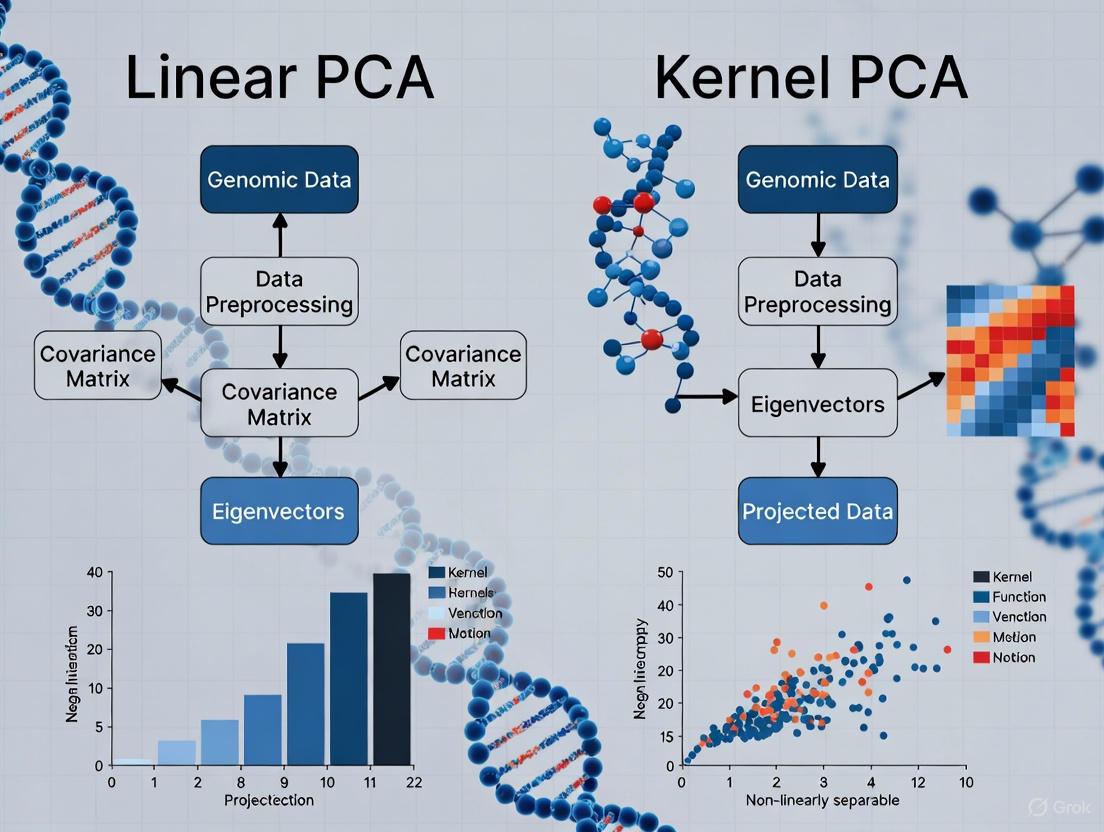
Workflow for Genomic Data Analysis Using PCA

The following diagram illustrates the standardized workflow for applying both linear and kernel PCA to genomic data, highlighting their divergent paths for handling linear versus non-linear patterns:

PCA Workflow for Genomic Data

Essential Computational Tools for Genomic PCA

Implementing PCA in genomic research requires specialized software tools capable of handling large-scale biological datasets while providing appropriate algorithmic variants for different data structures. The following table catalogs key software solutions and their capabilities for both linear and kernel PCA applications in genomic research:

Table 4: Computational Tools for PCA in Genomic Research

Tool	PCA Type	Key Features	Genomic Applications
VCF2PCACluster [9]	Linear	Memory-efficient (0.1GB for 81M SNPs), fast processing, clustering integration	Population structure analysis, large-scale SNP datasets
PLINK2 [9]	Linear	Established standard, comprehensive QC features, format conversion	Genome-wide association studies, population genetics
KSRV Framework [8]	Kernel PCA (RBF)	Spatial transcriptomics integration, RNA velocity inference	Cellular differentiation trajectories, developmental biology
KPCA with cforest [6]	Kernel PCA (ANOVA)	Random forest variable importance, metabolite identification	Metabolomics, biomarker discovery, nutritional studies
Scikit-learn [4]	Linear & Kernel PCA	Python implementation, versatile kernels, integration with ML pipelines	General-purpose genomic analysis, prototyping algorithms

Linear PCA remains an indispensable tool for genomic research, particularly for population structure analysis where its efficiency and interpretability provide significant advantages [9] [2]. Its linear assumptions, while limiting in some contexts, yield highly computationally efficient algorithms capable of processing tens of millions of SNPs with minimal memory requirements [9]. However, as genomic research increasingly addresses complex non-linear phenomena such as cellular differentiation, gene expression dynamics, and metabolic pathways, kernel PCA offers a powerful extension that can capture these sophisticated patterns [8] [6].

The choice between linear and kernel PCA should be guided by the specific research question, data characteristics, and computational resources. Linear PCA suffices for many population genetics applications where linear patterns dominate and interpretability is paramount [9]. In contrast, kernel PCA excels in contexts where biological systems exhibit inherent non-linearities, such as spatial transcriptomics and metabolomics, despite its greater computational demands and interpretive challenges [8] [6]. Future methodological developments will likely focus on hybrid approaches that balance efficiency with flexibility, along with improved interpretation techniques for non-linear component analyses [7] [6].

In the field of genomics, researchers routinely encounter datasets where the number of variables (p) vastly exceeds the number of observations (n), creating a significant p >> n problem. This high-dimensionality is further complicated by multicollinearity—extreme correlations between genetic variants due to linkage disequilibrium—which makes traditional statistical models unstable or impossible to fit [11] [12]. Genomic data from technologies like SNP microarrays or RNA sequencing can measure tens of thousands to millions of features (genes, SNPs) from only hundreds of samples. Principal Component Analysis (PCA) has emerged as a fundamental tool to address these challenges, with both linear and nonlinear (kernel) variants offering distinct approaches to dimensionality reduction in genomic studies [13] [14].

Linear vs. Kernel PCA: Core Methodological Differences

Linear PCA

Linear PCA is an unsupervised linear dimensionality reduction technique that projects data onto a new set of orthogonal axes called principal components [15]. These components are chosen to maximize the variance of the projected data, with the first component (PC1) capturing the largest possible variance, the second (PC2) capturing the next largest while being orthogonal to PC1, and so on [15]. The method works by performing an eigen decomposition of the covariance matrix of the centered data, with the eigenvectors defining the directions of the new components [15].

Kernel PCA (KPCA)

Kernel PCA extends linear PCA by applying the kernel trick to implicitly map data into a higher-dimensional feature space [16] [6]. This mapping allows KPCA to capture complex nonlinear relationships in the data that linear PCA would miss. After the transformation, standard PCA is performed in this new feature space, enabling the discovery of nonlinear patterns and structures [16]. The choice of kernel function—such as linear, polynomial, Gaussian (RBF), or sigmoid—provides flexibility in how the data is transformed [16].

The diagram below illustrates the conceptual difference between the two approaches:

Comparative Strengths and Limitations

Table 1: Methodological Comparison of Linear PCA and Kernel PCA

Feature	Linear PCA	Kernel PCA
Mathematical Foundation	Eigen decomposition of covariance matrix	Kernel trick + eigen decomposition of kernel matrix
Linearity Assumption	Assumes linear relationships in data	Captures nonlinear patterns and interactions
Computational Complexity	Lower complexity, suitable for large datasets	Higher complexity, especially for large sample sizes
Interpretability	Components are linear combinations of original variables	Interpretability challenging due to implicit mapping
Key Advantage	Computational efficiency, simplicity, interpretability	Flexibility in capturing complex data structures
Primary Limitation	Cannot capture nonlinear patterns	Computational demands, parameter selection complexity

Performance Comparison in Genomic Applications

Simulation Studies and Direct Comparisons

In a comprehensive simulation study specifically designed for high-dimensional genomic data integration, researchers found that the first few kernel principal components showed poorer performance compared to linear principal components for classification tasks [13]. The study developed a copula-based simulation algorithm that accounted for the degree of dependence and nonlinearity observed in real genomic datasets, then compared linear and kernel PCA methods for data integration and death classification [13]. Surprisingly, the results indicated that reducing dimensions using linear PCA with a logistic regression model provided adequate classification performance for genomic data, though integrating information from multiple datasets using either approach improved classification accuracy [13].

Genomic Prediction Performance

Research comparing principal component regression (PCR) with genomic REML (GREML) for genomic prediction across populations revealed that GREML slightly outperformed PCR in most scenarios [11] [12]. The study utilized pre-corrected average daily milk, fat, and protein yields of 1,609 first lactation Holstein heifers from Ireland, UK, the Netherlands, and Sweden, genotyped with 50k SNPs [12]. The highest achievable PCR accuracies were obtained across a wide range of principal components (from one to more than 1,000), but selecting the optimal number of components remained challenging [12].

Table 2: Experimental Performance in Genomic Studies

Study/Application	Linear PCA Performance	Kernel PCA Performance	Key Metrics
Genomic Data Integration [13]	Adequate for classification	Poor performance in first few components	Classification accuracy, AUC
Across-Population Genomic Prediction [12]	Slightly less accurate than GREML	Not evaluated	Prediction accuracy, correlation
Metabolite-Diet Association [6]	Limited pattern separation	Effective clustering by individual differences	Pattern separation, clustering quality
Cancer Classification [17]	Used in combination with other methods	Not evaluated	Classification accuracy

Successful Application of KPCA in Metabolomics

Despite generally mixed performance, KPCA has demonstrated notable success in specific genomic applications. In NMR-based metabolic profiling, KPCA effectively revealed nonlinear metabolic relationships that conventional PCA failed to capture [6]. The study incorporated a random forest conditional variable importance measure (cforest) to identify key metabolites following KPCA, successfully identifying hippurate as the most important variable associated with dietary patterns [6]. This KPCA-incorporated analytical approach enabled researchers to capture input-output responses between urinary metabolites and nutritional intake that remained hidden with linear methods [6].

Experimental Protocols and Methodologies

Standard PCA Protocol for Genomic Data

The typical workflow for applying linear PCA to genomic data involves several key steps [12]:

• Data Preparation: Format genotype data into a matrix X of order (n × p) where n individuals have been genotyped for p SNPs, with elements coded as 0, 1, or 2 representing homozygous reference, heterozygous, and homozygous alternative genotypes respectively.

• Data Standardization: Center the data by subtracting the mean of each variable, with optional scaling to unit variance.

• Covariance Matrix Computation: Calculate the covariance matrix (or correlation matrix) of the standardized genotype data.

• Eigen Decomposition: Perform eigen decomposition of the covariance matrix to obtain eigenvalues and eigenvectors.

• Component Selection: Choose the top k eigenvectors (principal components) based on eigenvalues (variance explained) or a predetermined threshold (e.g., 95% variance explained).

• Data Projection: Project the original data onto the selected principal components to obtain the transformed dataset: T = XW, where W contains the selected eigenvectors.

Kernel PCA Implementation Protocol

The workflow for Kernel PCA includes additional steps related to kernel selection and parameter tuning [16] [6]:

• Kernel Selection: Choose an appropriate kernel function based on data characteristics (linear, polynomial, Gaussian RBF, sigmoid).

• Parameter Tuning: Optimize kernel parameters (e.g., degree for polynomial kernels, sigma for Gaussian kernels) through cross-validation.

• Kernel Matrix Computation: Compute the kernel matrix K where each element Kij represents the similarity between subjects i and j based on the chosen kernel function.

• Center the Kernel Matrix: Modify the kernel matrix to ensure it represents data centered in the feature space.

• Eigen Decomposition: Perform eigen decomposition of the centered kernel matrix.

• Component Selection and Projection: Similar to linear PCA, but operating on the kernel matrix rather than the original data.

The following diagram illustrates the comparative experimental workflows:

The Scientist's Toolkit: Essential Research Reagents and Solutions

Table 3: Key Analytical Tools for Genomic Dimensionality Reduction

Tool/Technique	Function	Application Context
Linear PCA	Linear dimensionality reduction	Population stratification, noise reduction, multicollinearity resolution
Kernel PCA	Nonlinear dimensionality reduction	Capturing complex genetic interactions, metabolic pathway analysis
Random Forest cforest	Variable importance measurement	Identifying key biomarkers post-KPCA analysis [6]
Copula-based Simulation	Generating realistic genomic data	Method comparison accounting for genomic data structures [13]
Genomic Relationship Matrix (G matrix)	Quantifying genetic similarity	Mixed models replacing pedigree relationships [12]
Cross-validation Protocols	Model selection and validation	Determining optimal number of components [12]

The comparative analysis reveals that linear PCA remains a robust and efficient choice for many genomic applications, particularly when dealing with population structure, multicollinearity, and the p >> n problem [13] [12]. Its computational efficiency, interpretability, and generally adequate performance make it suitable for initial data exploration and dimensionality reduction in high-dimensional genomic studies.

Kernel PCA offers complementary strengths for specific scenarios where nonlinear patterns are theoretically important, such as in metabolic profiling or when analyzing complex gene-gene interactions [6]. However, its increased computational demands, parameter sensitivity, and challenging interpretation have limited its widespread adoption in genomics.

For researchers navigating these methodologies, the evidence suggests: (1) Begin with linear PCA for initial data exploration and dimensionality reduction; (2) Reserve kernel PCA for situations where nonlinear relationships are strongly suspected or initial linear approaches prove inadequate; (3) Consider hybrid approaches that combine PCA with machine learning methods like random forests for enhanced pattern detection [6]; and (4) Carefully validate the choice of dimensionality reduction method based on the specific analytical goals and data characteristics of each study.

The analysis of genomic data presents a fundamental challenge: the number of variables (e.g., SNPs, genes) vastly exceeds the number of observations (samples or cells), a phenomenon known as the "curse of dimensionality." Principal Component Analysis (PCA) has emerged as a ubiquitous solution to this problem, providing a robust mathematical framework for simplifying complex biological data while preserving essential patterns and structures. As a dimensionality reduction technique, PCA transforms high-dimensional genomic data into a smaller set of uncorrelated variables called principal components, which capture the maximum variance in the data [1]. This process enables researchers to visualize population structure, identify key quality control metrics, and uncover underlying biological relationships that would otherwise remain hidden in the high-dimensional space.

The recent advent of kernel PCA (KPCA) represents a significant evolution of traditional linear PCA, extending its capabilities to capture complex nonlinear relationships in data [18]. While linear PCA identifies principal components that are linear combinations of the original variables, KPCA utilizes the kernel trick to implicitly map data into a higher-dimensional feature space where nonlinear patterns become separable by linear methods. This theoretical advancement has profound implications for genomic research, where biological relationships often exhibit nonlinear characteristics. This article provides a comprehensive comparison of linear PCA and kernel PCA, examining their respective performances, applications, and methodological considerations within genomic research contexts, from population genetics to single-cell transcriptomics.

Theoretical Foundations: Linear PCA vs. Kernel PCA

Mathematical Underpinnings of Linear PCA

Principal Component Analysis operates on a simple yet powerful geometric principle: identifying the orthogonal directions (principal components) in which the data exhibits maximum variance. The algorithm follows a standardized computational pipeline [1]:

• Standardization: Centering and scaling the data to ensure each variable contributes equally to the analysis
• Covariance Matrix Computation: Calculating how variables vary from the mean relative to each other
• Eigen Decomposition: Determining eigenvectors (principal components) and eigenvalues (variance explained) from the covariance matrix
• Feature Selection: Retaining components that capture significant variance
• Data Projection: Transforming the original data onto the new principal component axes

The principal components are constructed as linear combinations of the initial variables, with the first component capturing the largest possible variance, the second component capturing the next highest variance while being uncorrelated with the first, and so on [1]. Geometrically, these components represent new axes that provide the optimal angle for visualizing and evaluating data differences.

Kernel PCA: Extending to Nonlinear Domains

Kernel PCA extends traditional PCA to capture nonlinear structures by leveraging the kernel trick, a mathematical approach that enables operations in high-dimensional feature spaces without explicit computation of coordinates [18]. The fundamental innovation of KPCA lies in its implicit mapping of original data points from their input space to a higher-dimensional feature space using a nonlinear function φ:

[ φ:ℝ^d→ℝ^D, D≫d ]

Instead of performing eigen-decomposition on the covariance matrix of the original data, KPCA works with the kernel matrix K, where each entry (K{ij} = k(xi,xj) = \langle φ(xi), φ(x_j)\rangle) represents the similarity between data points in this high-dimensional feature space [18]. Common kernel functions include the Radial Basis Function (RBF), polynomial, and sigmoid kernels, each imposing different geometric properties on the transformed feature space.

Table 1: Common Kernel Functions in Kernel PCA

Kernel Type	Mathematical Form	Key Parameters	Best Suited For
Radial Basis Function (RBF)	(k(xi,xj) = \exp(-\gamma ||xi-xj||^2))	γ (bandwidth)	Complex nonlinear structures
Polynomial	(k(xi,xj) = (xi \cdot xj + c)^d)	d (degree), c (coefficient)	Polynomial relationships
Sigmoid	(k(xi,xj) = \tanh(\alpha xi \cdot xj + c))	α, c	Neural network-like structures

Performance Comparison: Empirical Evidence Across Genomic Applications

Population Genetics and Ancestry Analysis

In population genetics, PCA has become the standard method for visualizing population structure and inferring ancestry patterns from genome-wide SNP data. Linear PCA efficiently identifies major population divergences, revealing genetic clusters that often correspond to geographic origins [19]. However, kernel PCA demonstrates superior capability in capturing fine-scale population structures and continuous gradients of genetic variation that may exhibit nonlinear patterns.

The performance of PCA in population genetics is heavily dependent on implementation considerations. VCF2PCACluster exemplifies modern optimized PCA tools, achieving identical accuracy to established software like PLINK2 and GCTA while demonstrating significantly better performance in memory usage (~0.1 GB versus >200 GB for 81.2 million SNPs) [9]. This memory efficiency stems from its line-by-line processing strategy, where memory usage depends solely on sample size rather than the number of SNPs, making it particularly suitable for large-scale genome-wide studies.

Table 2: Performance Comparison of PCA Tools for Genomic Analysis

Tool	Input Format	Key Features	Memory Usage	Computation Time
VCF2PCACluster	VCF	Kinship estimation, PCA, clustering, visualization	~0.1 GB (independent of SNP number)	~610 min for 81.2M SNPs
PLINK2	VCF/PLINK	General genetic analysis	>200 GB for 81.2M SNPs	Comparable to VCF2PCACluster
GCTA	VCF/BED	Heritability analysis, PCA	High	Similar to PLINK2
TASSEL	Multiple	Evolutionary genetics	>150 GB	>400 min
GAPIT3	Multiple	Genome-wide association study	>150 GB	>400 min

Single-Cell Transcriptomics and Spatial Genomics

In single-cell RNA sequencing (scRNA-seq) and spatial transcriptomics, kernel methods have demonstrated particular utility for tackling nonlinear relationships in cellular differentiation trajectories. The KSRV (Kernel PCA-based Spatial RNA Velocity) framework integrates scRNA-seq with spatial transcriptomics using Kernel PCA to accurately infer RNA velocity in spatially resolved tissues at single-cell resolution [8]. When validated using 10x Visium data and MERFISH datasets, KSRV showed superior accuracy and robustness compared to existing methods like SIRV and spVelo, successfully revealing spatial differentiation trajectories in the mouse brain and during mouse organogenesis [8].

The KSRV algorithm follows a systematic three-step process that highlights the practical application of kernel methods in genomic research [8]:

• Integration: scRNA-seq and spatial transcriptomics (ST) data are independently projected into a nonlinear latent space via kernel PCA with a radial basis function (RBF) kernel, followed by alignment using domain adaptation
• Prediction: Based on aligned latent representations, KSRV predicts spliced and unspliced expression at each spatial spot by borrowing information from nearby single cells using k-nearest neighbors (kNN) regression with k=50
• Velocity Estimation: With the enriched data, spatial RNA velocity vectors are estimated and used to reconstruct cell differentiation trajectories in space at single-cell resolution

Figure 1: KSRV Workflow for Spatial RNA Velocity Inference

Quality Control in Industrial and Manufacturing Applications

Beyond genomic research, PCA and kernel PCA play crucial roles in quality control and process monitoring, particularly in industrial applications where multivariate process data requires continuous surveillance. While conventional PCA effectively monitors linear processes, its kernel variant proves essential for detecting faults in systems with nonlinear characteristics [20].

In a comprehensive comparison of monitoring techniques for industrial processes like the Tennessee Eastman Process and Cement Rotary Kiln, Reduced KPCA (RKPCA) methods demonstrated significant advantages in fault detection accuracy while addressing KPCA's computational challenges [20]. These approaches utilize data reduction techniques like Spectral Clustering (SpC) and Random Sampling (RnS) to retain the most relevant observations, maintaining detection performance while reducing computation time and storage space by up to 70% compared to conventional KPCA [20].

For monitoring mixed attribute and variable quality characteristics, the Kernel PCA Mix Chart has shown superior performance compared to the PCA Mix Chart, particularly for detecting small mean shifts when categorical data has imbalanced proportions [21]. This capability is crucial for modern manufacturing, where 95% of products might have good quality while only 5% are defective, creating precisely the type of imbalanced scenario where kernel methods excel.

Experimental Protocols and Methodological Considerations

Standardized Protocol for Population Genetics PCA

For researchers implementing PCA in population genetic studies, the following protocol ensures reproducible results:

• Data Preprocessing: Filter SNPs based on missingness (>10% excluded), minor allele frequency (MAF < 0.05 excluded), and Hardy-Weinberg equilibrium (p < 10⁻⁶) [9]
• Kinship Matrix Calculation: Use normalizedIBS or centeredIBS methods to account for genetic relatedness and mitigate confounding factors [9]
• PCA Implementation: Execute eigen decomposition on the kinship matrix using optimized tools like VCF2PCACluster
• Component Selection: Retain components explaining >1% of variance each, or use scree plot inflection point
• Visualization: Generate 2D/3D plots of the first 2-3 principal components, coloring samples by putative populations
• Cluster Validation: Apply EM-Gaussian, K-Means, or DBSCAN clustering on top PCs and compare with known sample labels

Kernel PCA Implementation for Nonlinear Data

When implementing kernel PCA for genomic data with suspected nonlinear patterns, the following protocol is recommended:

• Kernel Selection: Choose an appropriate kernel function based on data characteristics:

  • RBF kernel for complex nonlinear structures (default γ = 1/(number of features × variance of data))
  • Polynomial kernel for known polynomial relationships
  • Sigmoid kernel for neural network applications [18]

• Parameter Optimization: Use grid search with cross-validation to identify optimal kernel parameters, as performance heavily depends on proper tuning [18]

• Computational Considerations: For large datasets (>10,000 samples), implement reduced KPCA approaches like SpC or RnS to maintain computational feasibility [20]

• Interpretation: Address the black-box nature of kernel methods using interpretation techniques like KPCA-IG (Interpretable Gradient), which computes feature importance based on partial derivatives of the kernel function [22]

The Scientist's Toolkit: Essential Research Reagents and Computational Solutions

Table 3: Essential Computational Tools for PCA in Genomic Research

Tool/Resource	Function	Application Context	Key Advantage
VCF2PCACluster	Kinship estimation, PCA, clustering	Population genetics	Memory efficiency independent of SNP number
KSRV Framework	Spatial RNA velocity inference	Single-cell/spatial transcriptomics	Nonlinear integration of scRNA-seq and spatial data
KPCA-IG	Feature interpretation in kernel PCA	High-dimensional omics data	Data-driven feature importance ranking
RKPCA with SpC/RnS	Fault detection in nonlinear processes	Quality control, process monitoring	Reduced computation while maintaining detection accuracy
Kernel PCA Mix Chart	Monitoring mixed quality characteristics	Industrial quality control	Superior performance with imbalanced categorical data

Discussion: Strategic Selection for Genomic Research Applications

The choice between linear PCA and kernel PCA depends fundamentally on the research question, data characteristics, and computational resources. Linear PCA remains the preferred method for initial data exploration, visualization of clear population structures, and quality control of large-scale genomic datasets where computational efficiency is paramount. Its advantages include computational efficiency, straightforward interpretation, and well-established methodologies [1].

Kernel PCA demonstrates superior performance in scenarios involving complex nonlinear relationships, such as cellular differentiation trajectories, subtle population substructures, and systems with strong interactive effects [8] [22]. The limitations of KPCA—including computational demands, sensitivity to kernel parameters, and interpretability challenges—are being actively addressed through methodological advances like reduced KPCA and interpretation frameworks like KPCA-IG [20] [22].

As genomic technologies continue to evolve, producing increasingly complex and high-dimensional data, the integration of kernel methods with traditional linear approaches will likely become standard practice. Frameworks like KSRV that strategically combine linear and nonlinear dimensionality reduction techniques point toward a future where researchers can flexibly adapt their analytical approach to the inherent structure of their biological data, ultimately leading to more accurate models of complex biological systems.

For researchers in genomics, analyzing high-dimensional data like single-cell RNA sequencing (scRNA-seq) results often means confronting complex, nonlinear relationships between variables. Traditional Principal Component Analysis (PCA), a linear method, can struggle to capture these intricate patterns, potentially obscuring meaningful biological insights [23] [24]. Kernel PCA (KPCA) addresses this fundamental limitation, offering a powerful nonlinear alternative that has become instrumental in advancing genomic research [8] [22].

The Core Principle: From Linear to Nonlinear Separation

The central idea behind KPCA is conceptually elegant: it uses a kernel function to implicitly map input data into a higher-dimensional feature space, where complex nonlinear structures in the original data become linearly separable. Principal components are then identified in this new space [23] [24].

This process relies on the "kernel trick," which allows the model to compute the inner products (a measure of similarity) in the high-dimensional feature space without ever needing to calculate the coordinates of the data in that space explicitly [22]. This makes the computation feasible, even for very high-dimensional genomic data.

The following diagram illustrates the conceptual workflow of KPCA compared to linear PCA.

The Mathematical Foundation

The kernel trick transforms the data matrix. Let a dataset of ( n ) observations be ( \mathbf{x}1, \ldots, \mathbf{x}n ) with ( \mathbf{x}_i \in \mathbb{R}^p ). A kernel function ( k ) is defined as ( k: \chi \times \chi \longrightarrow \mathbb{R} ), which must be symmetric and positive semi-definite [22].

KPCA operates on the kernel matrix ( \mathbf{K} ), where each element ( \mathbf{K}{ij} = k(\mathbf{x}i, \mathbf{x}_j) ) represents the pairwise similarity between data points ( i ) and ( j ) in the high-dimensional feature space [22]. The principal components in this space are obtained by solving an eigenvalue problem on the centered kernel matrix ( \tilde{\mathbf{K}} ) [22].

Kernel Functions in Practice

The choice of kernel function determines the type of nonlinear relationships the model can capture. The table below summarizes common kernels used in genomic studies.

Table 1: Common Kernel Functions in KPCA

Kernel Name	Mathematical Form	Key Characteristics	Typical Use Cases in Genomics
Radial Basis Function (RBF)	( K(\mathbf{x}i, \mathbf{x}j) = \exp(-\gamma |\mathbf{x}i - \mathbf{x}j|^2) )	Captures local, complex nonlinear structures; highly flexible [8] [24].	Analyzing data with intricate, local patterns like cellular differentiation trajectories [8].
Polynomial	( K(\mathbf{x}i, \mathbf{x}j) = (\mathbf{x}i \cdot \mathbf{x}j + c)^d )	Captures global, polynomial relationships; complexity controlled by degree ( d ) [24].	Useful for feature interactions that can be modeled by polynomial functions.

KPCA vs. Linear PCA: A Performance Benchmark

The theoretical advantage of KPCA is best understood through its performance in practical genomic applications. The following examples demonstrate its superiority over linear PCA in handling nonlinear data structures.

Case Study: The Swiss Roll Dataset

The "Swiss Roll" is a classic example of a simple 3D manifold where the true underlying structure is a 2D spiral. When linear PCA is applied, it fails to "unroll" the spiral, instead projecting the data in a way that retains the spiral shape and leaves different sections linearly inseparable [24]. In contrast, KPCA using an RBF kernel successfully unrolls the manifold, clearly separating the different sections of the spiral and revealing the true, simpler structure of the data [24].

Case Study: Spatial Transcriptomics and RNA Velocity

A direct benchmark in a cutting-edge genomic application comes from the KSRV framework, a method for inferring spatial RNA velocity. KSRV integrates scRNA-seq data with spatial transcriptomics data using KPCA. The developers validated KSRV on 10x Visium and MERFISH datasets, showing it was more accurate and robust at revealing spatial differentiation trajectories in the mouse brain and during mouse organogenesis compared to existing methods like SIRV and spVelo, which may rely on linear assumptions [8]. This demonstrates KPCA's power in integrating complex, multi-modal genomic data to uncover dynamic biological processes.

Quantitative Performance Comparisons

The table below summarizes key findings from benchmarks comparing dimensionality reduction techniques, including PCA and its alternatives.

Table 2: Benchmarking Dimensionality Reduction Techniques

Method	Reported Performance / Characteristics	Context / Dataset
Kernel PCA (KPCA)	Successfully revealed spatial differentiation trajectories; more accurate/robust than SIRV/spVelo [8].	Spatial RNA velocity inference (10x Visium, MERFISH) [8].
Random Projections (RP)	Surpassed PCA in computational speed; rivaled or exceeded PCA in preserving data variability and clustering quality [25].	Benchmarking on scRNA-seq datasets [25].
Standard PCA	Performance typically degrades with increasing data size; sensitive to outliers; assumes linearity [25].	General limitation noted in benchmarking study [25].

Experimental Protocols for Genomic Data

Implementing KPCA effectively on genomic data requires a structured workflow. The following diagram and protocol detail the key steps, drawing from methodologies used in recent studies.

Detailed Methodology for Spatial RNA Velocity Inference (KSRV)

The KSRV framework provides a clear protocol for using KPCA with genomic data [8]:

• Data Integration and Domain Adaptation: Begin with scRNA-seq and spatial transcriptomics (ST) data. Identify a common gene set and apply a domain adaptation framework (like PRECISE) to align the distributions of the two datasets and mitigate batch effects before dimensionality reduction [8].
• Nonlinear Projection with Kernel PCA: Independently project both the scRNA-seq and ST data into a shared nonlinear latent space using Kernel PCA with an RBF kernel. Compute the eigenvectors of the kernel matrices to extract principal components [8].
• Latent Space Alignment: Apply singular value decomposition (SVD) to orthogonalize the components from the two datasets. Retain only those components with a cosine similarity exceeding a defined threshold (e.g., 0.3) to finalize the common latent space [8].
• Prediction and Imputation: For each spot in the spatial data, predict its unmeasured spliced and unspliced gene expression. This is done by performing a k-nearest neighbors (kNN) regression (e.g., k=50) on its nearest neighbors from the aligned scRNA-seq data in the latent space, using a weighted average based on cosine distance [8].
• Velocity Calculation and Trajectory Inference: Using the imputed expression values, compute RNA velocity vectors for each spatial cell. Project these vectors onto the tissue's spatial coordinates to visualize and reconstruct cell differentiation trajectories [8].

The Researcher's Toolkit for KPCA

Table 3: Essential Research Reagent Solutions for KPCA in Genomics

Tool / Resource	Function / Description	Relevance to KPCA
scRNA-seq Data (e.g., from 10X Genomics)	Provides high-resolution, single-cell gene expression profiles.	Serves as a foundational data source for integration with spatial data using frameworks like KSRV [8].
Spatial Transcriptomics Data (e.g., 10x Visium, MERFISH)	Provides gene expression data with preserved spatial context within a tissue.	The key dataset for which KPCA helps infer dynamics (e.g., RNA velocity) [8].
RBF Kernel	A kernel function to measure nonlinear similarity between data points.	The core function that enables KPCA to capture complex, nonlinear patterns in genomic data [8] [24].
KSRV Framework	A computational framework for inferring spatial RNA velocity.	A specific, validated implementation of KPCA for a pressing genomic challenge [8].
Domain Adaptation Tools (e.g., PRECISE)	Methods to align data distributions from different sources or technologies.	Critical pre-processing step for integrating diverse genomic datasets (e.g., scRNA-seq and ST) before applying KPCA [8].
k-Nearest Neighbors (kNN) Regression	An algorithm used for prediction based on local neighbors in a latent space.	Used in conjunction with KPCA to impute missing gene expression values in spatial data [8].

In the analysis of high-dimensional genomic data, the limitations of linear PCA are becoming increasingly apparent. Kernel PCA provides a mathematically sound and practically validated framework for uncovering the nonlinear patterns that define cellular heterogeneity, differentiation, and spatial organization. As genomic technologies continue to generate data of increasing complexity and scale, leveraging nonlinear alternatives like KPCA will be crucial for researchers and drug developers aiming to extract the most profound biological insights from their data.

In the field of genomic research, where data dimensionality is exceptionally high and biological relationships are often nonlinear, kernel functions have emerged as a powerful mathematical framework for data transformation and analysis. Kernel methods operate on a fundamental principle: they implicitly map data from its original input space into a higher-dimensional feature space where complex, nonlinear patterns become linearly separable. This "kernel trick" allows researchers to perform sophisticated analyses without explicitly computing the coordinates in the higher-dimensional space, making computationally intensive genomic analyses feasible. Within this framework, Linear, Polynomial, and Radial Basis Function (RBF) kernels represent the most widely adopted approaches, each with distinct characteristics that make them suitable for different genomic scenarios. The application of these kernels extends beyond classification to include dimensionality reduction through Kernel Principal Component Analysis (KPCA), which provides a nonlinear alternative to standard PCA and can more effectively capture the complex manifold of biological sample spaces [22].

The selection of an appropriate kernel function is particularly crucial in genomics, where the choice influences the model's ability to capture the underlying biological reality. As we compare these fundamental kernels, it's important to recognize that they form the foundation for more advanced methods now being developed for single-cell and multi-omics integration, such as Multiple Kernel Learning (MKL) frameworks that can transparently model both transcriptomic and epigenomic modalities [26]. This guide provides a systematic comparison of Linear, Polynomial, and RBF kernels specifically within the context of genomic data transformation, offering researchers evidence-based guidance for method selection.

Kernel Functions: Mathematical Foundations and Biological Interpretations

Core Kernel Concepts

Kernel functions fundamentally measure the similarity between pairs of data points based on their genomic features. Mathematically, a kernel function ( k(\mathbf{xi}, \mathbf{xj}) ) computes the inner product between two data points ( \mathbf{xi} ) and ( \mathbf{xj} ) after they have been transformed by a feature mapping function ( \phi ) that projects them into a higher-dimensional space: ( k(\mathbf{xi}, \mathbf{xj}) = \langle \phi(\mathbf{xi}), \phi(\mathbf{xj}) \rangle ). The requirement for a valid kernel is that it must be symmetric and positive semi-definite, ensuring a solid statistical foundation for its use in penalized regression models [14]. This mathematical framework allows genomic researchers to work with similarity measures between samples rather than explicit coordinate representations, which is particularly advantageous when dealing with the high dimensionality of genomic data where the number of features (genes, SNPs, etc.) often vastly exceeds the number of observations.

The biological interpretation of kernel functions relates to how they quantify functional or structural relationships between biological samples. In genome-wide association studies (GWAS), for instance, kernels can be designed to reflect shared genetic variation, while in gene expression analysis, they might capture coordinated expression patterns. The kernel matrix (or Gram matrix) generated by applying a kernel function to all pairs of samples in a dataset effectively encodes a similarity network of biological samples, which can then be used for various analyses including classification, regression, clustering, and dimensionality reduction. This network perspective aligns well with the complex interconnected nature of biological systems.

Kernel Functions for Genomic Data

Table 1: Comparison of Primary Kernel Functions for Genomic Data

Kernel Type	Mathematical Formulation	Key Parameters	Genomic Interpretation	Ideal Use Cases
Linear	( k(\mathbf{xi}, \mathbf{xj}) = \mathbf{xi}^T \mathbf{xj} )	None	Measures simple covariance between genomic profiles	Linearly separable data, high-dimensional datasets, baseline comparisons
Polynomial	( k(\mathbf{xi}, \mathbf{xj}) = (1 + \mathbf{xi}^T \mathbf{xj})^d )	Degree (d), Coefficient (c)	Captures multiplicative interaction effects between genomic features	Modeling pathway interactions, epistasis in genetics, higher-order feature combinations
RBF (Gaussian)	( k(\mathbf{xi}, \mathbf{xj}) = \exp\left(-\frac{|\mathbf{xi} - \mathbf{xj}|^2}{2\sigma^2}\right) )	Bandwidth (γ), where ( \gamma = \frac{1}{2\sigma^2} )	Creates local similarity neighborhoods based on exponential decay of similarity with distance	Capturing complex nonlinear relationships, clustering similar expression patterns, most biological datasets
Weighted Linear	( k(\mathbf{xi}, \mathbf{xj}) = \sum{k=1}^q wk G{ik} G{jk} )	Weights ( w_k ) for each SNP/feature	Gives greater importance to rarer genetic variants when sharing rare alleles	GWAS studies, population genetics, familial relatedness

The Linear Kernel represents the simplest approach, computing a standard dot product between two sample vectors. It assumes a linear relationship between genomic features and the outcome of interest, making it computationally efficient and less prone to overfitting, though it may fail to capture complex biological interactions. In practice, linear kernels work well for genomic datasets where the number of features already provides sufficient representational power, or when seeking a computationally efficient baseline model.

The Polynomial Kernel introduces nonlinearity by computing the d-th degree polynomial of the linear dot product. The degree parameter (d) controls the complexity of interactions the kernel can capture—with degree 2 capturing pairwise interactions, degree 3 capturing three-way interactions, and so on. This makes polynomial kernels particularly suitable for modeling biological phenomena like epistasis in genetics or pathway interactions in transcriptomics, where the combined effect of multiple genomic features is not merely additive [14].

The Radial Basis Function (RBF) Kernel, also known as the Gaussian kernel, takes a different approach by measuring similarity as an exponentially decaying function of the Euclidean distance between samples. The γ parameter (or bandwidth) controls the influence range of a single sample—small values create a broader influence, while large values create tighter, more localized similarity neighborhoods. The RBF kernel is particularly powerful for genomic data because it can capture complex nonlinear relationships without explicitly defining their functional form, making it suitable for most biological datasets where the true underlying relationship is unknown [14] [27].

Experimental Comparison: Benchmarking Kernel Performance on Genomic Data

Experimental Protocol for Kernel Evaluation

To objectively compare kernel performance on genomic data, researchers must implement a standardized evaluation protocol. A robust experimental framework includes the following key components:

• Dataset Selection and Preparation: Utilize diverse genomic datasets representing different biological contexts (e.g., gene expression, SNP data, epigenomic markers). The datasets should vary in key characteristics including number of features, sample size, and biological complexity. Prior to analysis, perform data scaling and normalization as kernel performance, particularly for linear kernels, can be significantly impacted by feature scales [28].

• Kernel Implementation: Apply each kernel function to transform the genomic data. For linear kernels, use the direct dot product implementation. For polynomial kernels, test multiple degree values (typically 2, 3, and 4) to capture different interaction levels. For RBF kernels, employ a range of γ values, often determined through cross-validation.

• Dimensionality Reduction and Analysis: Apply Kernel PCA to each transformed dataset to visualize the data structure in reduced dimensions. For classification tasks, implement Support Vector Machines (SVM) with each kernel type.

• Evaluation Metrics: Quantify performance using multiple metrics including:

  • Classification Accuracy: Area Under the Receiver Operating Characteristic Curve (AUROC) for classification tasks
  • Computational Efficiency: Training time and memory usage
  • Representation Quality: Variance explained in KPCA, cluster separation metrics

• Statistical Validation: Implement repeated train-test splits (e.g., 100 repetitions of 80/20 splits) with cross-validation to optimize hyperparameters and ensure robust performance estimates [26].

Quantitative Performance Comparison

Benchmarking studies across diverse genomic datasets reveal consistent patterns in kernel performance. The following table summarizes key findings from multiple genomic studies comparing kernel functions:

Table 2: Experimental Performance Comparison Across Genomic Datasets

Study Context	Best Performing Kernel	Performance Metric	Linear Kernel	Polynomial Kernel	RBF Kernel	Key Findings
Single-cell Multiomics Classification [26]	RBF	AUROC	0.82-0.89	0.85-0.91	0.89-0.94	RBF consistently outperformed linear across multiple cancer types (breast, prostate, lung)
Spatial RNA Velocity Inference (KSRV) [8]	RBF	Trajectory Accuracy	N/A	N/A	Superior	RBF-based KPCA effectively captured nonlinear spatial gene expression patterns
Genomic Prediction [29]	Non-parametric Methods	Pearson's r	0.62 (mean)	N/A	+0.014-0.025 improvement	Non-linear methods showed modest but significant gains over linear alternatives
Scintillation Detection [27]	Fine Gaussian (RBF)	Detection Accuracy	Lowest	Medium	Highest	Fine Gaussian SVM outperformed linear and polynomial kernels in complex signal detection
Computational Efficiency [28]	Linear (with scaling)	Training Time	0.0021s (scaled)	Hours (unscaled)	0.0039s (scaled)	Data scaling dramatically improved linear kernel performance (from 0.8672s to 0.0021s)

The experimental evidence consistently demonstrates that RBF kernels generally achieve superior performance for most genomic applications, particularly when capturing complex nonlinear relationships present in biological systems. In single-cell multiomics classification, scMKL utilizing RBF kernels achieved AUROC values between 0.89-0.94, outperforming linear kernels which ranged from 0.82-0.89 across breast, prostate, and lung cancer datasets [26]. Similarly, in the KSRV framework for spatial transcriptomics, RBF-based Kernel PCA successfully revealed spatial differentiation trajectories in the mouse brain and during mouse organogenesis by effectively modeling nonlinear relationships [8].

However, linear kernels maintain important advantages in specific scenarios. With proper data scaling, linear kernels can achieve competitive performance with significantly reduced computational requirements—in some benchmarks training 7× faster and using 12× less memory than more complex alternatives [26]. This makes linear kernels particularly valuable for initial exploratory analysis, extremely high-dimensional genomic data, or when computational resources are constrained.

Polynomial kernels occupy a middle ground, offering better performance than linear kernels for capturing multiplicative interactions while generally being more computationally intensive than RBF kernels. Their performance is highly dependent on proper parameter tuning, particularly the degree parameter which should be aligned with the expected complexity of biological interactions in the system under study.

Kernel PCA vs. Linear PCA: A Genomic Perspective

The fundamental difference between linear PCA and kernel PCA lies in their approach to dimensionality reduction. Linear PCA identifies linear directions of maximum variance in the original data space, while kernel PCA first projects data into a higher-dimensional feature space via a kernel function, then performs linear PCA in that space. This enables kernel PCA to capture nonlinear patterns that would be inaccessible to standard PCA.

In genomic applications, this distinction has profound implications. As noted in benchmark studies, "the relationships between the variables may be nonlinear, making linear methods unsuitable. Hence, with high-dimensional data such as genomic data, where the number of features is usually much larger than the number of samples, nonlinear methods like kernel methods can provide a valid alternative for data analysis" [22]. Kernel PCA has proven particularly valuable for spatial transcriptomics analysis, where it enables accurate inference of RNA velocity in spatially resolved tissue at single-cell resolution by capturing nonlinear gene expression dynamics [8].

However, kernel PCA introduces interpretability challenges. The original features are summarized in pairwise kernel similarity scores, making it difficult to identify which genomic features drive the observed patterns. Recent methodological advances like KPCA Interpretable Gradient (KPCA-IG) address this limitation by computing partial derivatives of the kernel to identify influential variables, providing a data-driven feature importance ranking specifically designed for high-dimensional genomic datasets [22].

Implementing kernel methods effectively for genomic analysis requires both computational tools and biological knowledge resources. The following table outlines key solutions and their applications:

Table 3: Essential Research Reagent Solutions for Genomic Kernel Applications

Resource Category	Specific Solutions	Function/Purpose	Genomic Application Examples
Computational Frameworks	scMKL [26], KSRV [8], ktest [30]	Specialized kernel methods for single-cell and spatial genomics	Multiomics integration, spatial trajectory inference, differential analysis
Kernel Implementations	SVM (scikit-learn), KPCA (scikit-learn), KernelRidge	General-purpose kernel method implementations	Baseline comparisons, custom analysis pipelines, method development
Biological Knowledge Bases	Hallmark Gene Sets (MSigDB), JASPAR, Cistrome [26]	Curated biological pathways and regulatory information	Biologically-informed kernel construction, pathway-centric analysis
Benchmarking Resources	EasyGeSe [29]	Curated genomic datasets for method validation	Performance benchmarking across diverse species and traits
Interpretability Tools	KPCA-IG [22]	Feature importance ranking for kernel PCA	Identification of influential genomic features in nonlinear analysis

Specialized computational frameworks like scMKL (Single-Cell Multiple Kernel Learning) have been specifically designed to address the unique challenges of genomic data, integrating both transcriptomic and epigenomic modalities while maintaining interpretability through group Lasso regularization [26]. Similarly, KSRV (Kernel PCA-based Spatial RNA Velocity) implements kernel PCA with RBF kernels to infer developmental trajectories from spatial transcriptomics data [8].

For biologically-informed analysis, leveraging curated knowledge bases is essential. The Molecular Signature Database (MSigDB) provides Hallmark gene sets that can guide kernel construction for transcriptomic data, while JASPAR and Cistrome offer transcription factor binding site information for epigenomic analysis [26]. These resources enable researchers to move beyond generic kernel functions to construct biologically meaningful similarity measures that reflect known regulatory relationships.

Benchmarking resources like EasyGeSe provide curated collections of genomic datasets across multiple species, enabling systematic evaluation of kernel methods and ensuring robust, generalizable performance [29]. As new kernel methods are developed, such resources become increasingly important for objective comparison and validation.

The comparative analysis of kernel functions for genomic data transformation reveals a consistent pattern: while RBF kernels generally provide superior performance for capturing complex biological relationships, linear kernels maintain value for computationally efficient analysis of high-dimensional data, particularly when properly scaled. Polynomial kernels offer a middle ground for capturing specific interaction effects but require careful parameter tuning.

The choice between linear and kernel PCA ultimately depends on the research question and data characteristics. For initial exploration or when biological relationships are expected to be primarily linear, standard PCA provides interpretable results with computational efficiency. For capturing complex nonlinear patterns in gene expression, spatial organization, or cellular trajectories, kernel PCA with RBF kernels offers significantly enhanced capability, albeit with increased computational demands and interpretability challenges.

Future directions in genomic kernel methods point toward multiple kernel learning approaches that integrate diverse data types and biological knowledge, interpretability enhancements that bridge the gap between complex models and biological insight, and scalability improvements that enable application to increasingly large genomic datasets. As single-cell and spatial technologies continue to advance, kernel methods will play an increasingly important role in unraveling the complex, nonlinear relationships that define biological systems, ultimately accelerating discoveries in basic science and therapeutic development.

From Theory to Practice: Implementing PCA and KPCA on Genomic Datasets

A Step-by-Step Workflow for Linear PCA on Genotype Matrices

Principal Component Analysis (PCA) remains a cornerstone technique for visualizing population structure and correcting for confounding in genomic studies. While kernel PCA offers advantages for capturing complex non-linear relationships, linear PCA maintains critical importance for its computational efficiency, straightforward interpretation, and well-established theoretical foundations in genetics. The leading principal components of genomic relationship matrices effectively capture genetic relatedness and population stratification, with the first few components typically sufficient for visualizing overarching population structures [31]. This guide provides a detailed workflow for implementing linear PCA on genotype matrices, objectively compares its performance with kernel alternatives, and presents experimental data to inform method selection for genomic research.

Theoretical Foundation: Linear PCA vs. Kernel PCA in Genomics

Linear PCA for Genomic Data

Linear PCA operates by identifying orthogonal directions of maximum variance in the original feature space of genotype data. For a centered genotype matrix X ∈ ℝ^n×p (with n individuals and p markers), PCA performs an eigen decomposition of the covariance matrix C = (1/(n-1))X^⊤X, or equivalently, a singular value decomposition (SVD) of X itself [32]. The resulting principal components (PCs) are linear combinations of the original genotypes that capture genetic variation in decreasing order. The projection of sample i onto PC k is given by t_ki = v_k^⊤x_i, where v_k is the k-th eigenvector [32]. In population genetics, these projections often correspond to geographic ancestry or breeding patterns when applied to genome-wide data.

Kernel PCA for Capturing Non-Linear Patterns

Kernel PCA extends this concept by first projecting genotypes into a higher-dimensional feature space via a non-linear mapping φ(x), then performing linear PCA in this transformed space [33]. This enables capture of complex patterns beyond simple covariance structures. The kernel trick allows this without explicitly computing φ(x) by working with the kernel matrix K where K_ij = k(x_i, x_j) = ⟨φ(x_i), φ(x_j)⟩, representing similarity between samples i and j in the transformed space [30]. Common kernel functions include radial basis function (RBF) and polynomial kernels. In genomics, this enables identification of subtle population structures and complex differentiation patterns that may not align with simple linear axes of variation.

Comparative Advantages in Genomic Context

Table 1: Theoretical Comparison of Linear and Kernel PCA for Genomic Data

Feature	Linear PCA	Kernel PCA
Computational Complexity	O(min(nk2, n2k)) for truncated SVD [31]	Higher due to kernel matrix computation and decomposition
Interpretability	High - PCs are linear combinations of original genotypes	Reduced - Components in feature space lack direct genetic interpretation
Memory Requirements	Moderate - Works with genotype matrix or covariance	High - Requires storing n×n kernel matrix
Handling of Non-Linear Patterns	Limited to linear relationships	Excellent for complex population structures
Implementation Maturity	Extensive tools and established best practices	Emerging methods with ongoing development

Experimental Comparison: Performance Benchmarks

Computational Efficiency

Recent benchmarks demonstrate substantial advantages of optimized linear PCA implementations for large-scale genomic data. The randPedPCA package enables rapid pedigree PCA using sparse matrix representations, achieving a speed-up greater than 10,000 times compared to naive PCA implementations [31]. This efficiency allows analysis of extremely large pedigrees, exemplified by processing the UK Kennel Club registered Labrador Retriever population of almost 1.5 million individuals [31].

For genotype data, linear PCA implementations leveraging randomized SVD algorithms show similar scalability advantages. The SF-GWAS framework implements secure federated PCA for genome-wide association studies, successfully processing UK Biobank-scale datasets of 410,000 individuals while maintaining practical runtimes [34]. These results underscore the maturity of linear PCA for biobank-scale genomic datasets.

Biological Relevance and Accuracy

Table 2: Empirical Performance Comparison on Genomic Datasets

Method	Dataset	Performance Metrics	Key Findings
Linear PCA (randPedPCA)	Simulated pedigree data	>10,000× speed-up vs. naive PCA [31]	Enables analyses impossible with naive PCA
Linear PCA (SF-GWAS)	UK Biobank (n=410,000)	5.3 days total runtime [34]	Practical for biobank-scale datasets
Kernel PCA (KSRV)	Mouse brain spatial transcriptomics	Superior to SIRV and spVelo methods [33]	Accurately reveals spatial differentiation trajectories
Kernel PCA (ktest)	Single-cell ChIP-Seq data	Identifies epigenomic heterogeneity [30]	Detects subtle population variations missed by other methods

Kernel PCA demonstrates particular strength in applications requiring capture of complex differentiation patterns. The KSRV framework, which employs kernel PCA to integrate single-cell RNA-seq with spatial transcriptomics, successfully revealed spatial differentiation trajectories in mouse brain and during mouse organogenesis [33]. Similarly, the ktest package applies kernel Fisher discriminant analysis to single-cell epigenomic data, identifying pre-existing subpopulations of breast cancer cells with persister-like epigenomic profiles prior to treatment [30]. These results highlight kernel PCA's advantage for detecting subtle biological variations in complex cellular systems.

Step-by-Step Workflow for Linear PCA on Genotype Matrices

Data Preprocessing and Quality Control

Genotype Encoding and Standardization: Raw genotype data should be encoded as 0, 1, 2 representing allele counts, then centered and scaled to ensure each marker contributes equally to the covariance structure. For a genotype matrix X, centering is typically performed by subtracting mean allele frequencies: W = X - 2p, where p is the vector of allele frequencies [34]. Some implementations further scale by √[2p_j(1-p_j)] to standardize by expected variance under Hardy-Weinberg equilibrium.

Quality Control Procedures: Prior to PCA, implement standard genomic QC filters: exclude markers with high missingness rates (>5%), significant deviation from Hardy-Weinberg equilibrium (p < 10^-6), and low minor allele frequency (MAF < 0.01). Sample-level QC should exclude individuals with excessive missing data (>10%) and identify unexpected duplicates or related individuals [34]. These steps ensure technical artifacts don't dominate the principal components.

Core PCA Implementation

Algorithm Selection: For large genotype matrices (n > 10,000), randomized SVD algorithms provide the best balance of computational efficiency and accuracy. These algorithms approximate the top principal components without computing the full covariance matrix, using random projections to identify the subspace containing the dominant eigenvectors [31]. When only a few leading PCs are needed (typically the case for population structure visualization), randomized methods can halve the running time required compared to traditional approaches [31].

Variance Standardization: For visualization of population structure, use the genotype correlation matrix rather than covariance matrix, which equalizes contributions across markers with different allele frequencies. This approach prevents rare variants from having disproportionate influence on the leading components and better captures true population signals.

Figure 1: Linear PCA workflow for genotype data

Special Considerations for Large Pedigrees

For pedigree data represented by the additive relationship matrix A, efficient PCA can be performed without explicitly constructing this dense matrix by leveraging the sparse Cholesky factor L^-1 of A^-1 [31]. The randPedPCA package implements this approach, enabling matrix-vector multiplications with A through solving triangular systems with L^-1, requiring only O(n) operations [31]. This allows PCA on pedigrees with millions of individuals using standard computational resources.

Advanced Methodological Considerations

Handling Missing Data in Ancient DNA

Ancient DNA datasets present unique challenges with extreme missingness (often <1% of SNPs observed). Standard PCA projection methods like SmartPCA can produce misleading results when missingness patterns correlate with true population structure [32]. The TrustPCA framework addresses this by quantifying projection uncertainty through a probabilistic model that estimates the distribution of possible PC coordinates given the observed SNPs [32]. This approach reveals when PCA placements are statistically robust versus highly uncertain due to sparse data.

Federated PCA for Privacy-Preserving Analysis

Multi-institutional genomic studies require privacy-preserving methods. SF-GWAS implements secure federated PCA using a hybrid homomorphic encryption and secure multiparty computation framework [34]. This approach performs PCA on distributed datasets without sharing raw genotypes, achieving runtimes of 44 hours for UK Biobank-scale data (n=275,812) while providing cryptographic privacy guarantees [34]. Federated PCA produces results virtually identical to pooled analysis, overcoming limitations of meta-analysis approaches that can produce biased results with heterogeneous datasets [34].

Dimensionality Reduction for Genomic Prediction

In genomic selection, PCA and other dimensionality reduction methods serve as valuable pre-processing steps before prediction modeling. Studies evaluating DR for genomic prediction found that only a fraction of features was sufficient to achieve maximum prediction accuracy, regardless of the DR method used [35]. This suggests that carefully implemented linear PCA can capture most genetically relevant variation while dramatically reducing computational demands for downstream prediction tasks.

The Scientist's Toolkit: Essential Research Reagents

Table 3: Key Software Tools for Genomic PCA Implementation

Tool	Function	Application Context
randPedPCA (R)	Rapid pedigree PCA using sparse matrices	Large pedigree visualization [31]
SF-GWAS	Secure federated PCA for GWAS	Multi-institutional genomic studies [34]
TrustPCA	Uncertainty quantification for PCA projections	Ancient DNA with extensive missingness [32]
KSRV	Kernel PCA for spatial transcriptomics	Spatial RNA velocity inference [33]
ktest	Kernel testing for single-cell differential analysis	Identifying subtle population heterogeneity [30]
PLINK	Standardized genotype QC and PCA	General population genetics [34]

Linear PCA remains an indispensable tool for genomic data exploration, offering unmatched computational efficiency and straightforward interpretability for standard population structure analysis. The development of optimized algorithms like randomized SVD and sparse matrix operations has maintained its relevance for biobank-scale datasets. Kernel PCA provides complementary strengths for capturing complex non-linear patterns in single-cell and spatial transcriptomics, where subtle biological variations are of primary interest. Method selection should be guided by dataset scale, biological question, and computational resources, with linear PCA representing the optimal starting point for most standard genomic applications and kernel PCA reserved for specialized applications requiring detection of complex structures.

In genomic data research, characterized by high-dimensional and often non-linear data structures, Principal Component Analysis (PCA) has long been a foundational tool. Traditional linear PCA reduces dimensionality by finding orthogonal directions of maximum variance in the original input space, making it powerful for revealing population structure and correcting for stratification in genetic studies [12]. However, its fundamental limitation is the assumption of linearity, which can prevent it from capturing complex, non-linear relationships between genetic markers—a common scenario in real biological systems [36].

Kernel PCA (KPCA) overcomes this limitation by using the "kernel trick" to perform a nonlinear mapping of the data into a high-dimensional feature space before applying standard PCA [36] [21]. Within this feature space, complex nonlinear structures in the original data can become linear and more easily separable. This capability is critical for genomics, where interactions between genes and their environment are rarely linear. KPCA provides a robust nonlinear alternative for dimensionality reduction, enabling researchers to uncover patterns and structures in genomic data that would remain hidden to linear methods [8] [36].

Core Principles: The Kernel Trick in PCA

The mathematical foundation of KPCA rests on mapping the original input data to a higher-dimensional feature space. Given a dataset of ( n ) observations ( \mathbf{x}1, \dots, \mathbf{x}n ) with ( \mathbf{x}_i \in \mathbb{R}^p ), a kernel function ( k ) is defined as ( k: \chi \times \chi \longrightarrow \mathbb{R} ), where the input set ( \chi ) is ( \mathbb{R}^p ) [36]. This function must be symmetric and positive semi-definite.

The power of the method comes from the implicit definition of a mapping function ( \phi ) that projects an input vector ( \mathbf{x} ) into a feature space ( \mathcal{H} ), such that the kernel computes a dot product in that space: ( k(\mathbf{x}i, \mathbf{x}j) = \langle \phi(\mathbf{x}i), \phi(\mathbf{x}j) \rangle ) [36]. Critically, the mapping ( \phi ) is never explicitly computed, which is computationally prohibitive for high-dimensional feature spaces. Instead, all operations are performed through the kernel matrix ( \mathbf{K} ), whose elements are ( K{ij} = k(\mathbf{x}i, \mathbf{x}_j) ) [36] [21]. This is the essence of the kernel trick, allowing KPCA to efficiently operate in a very high-dimensional (or even infinite-dimensional) feature space.

Kernel Selection: A Practical Guide for Genomic Data

The choice of kernel function fundamentally determines the feature space in which the data will be analyzed and thus the types of patterns KPCA can discover. The table below summarizes common kernels and their suitability for genomic data.

Table 1: Kernel Functions and Their Properties for Genomic Data

Kernel Type	Mathematical Form	Key Advantages	Genomic Data Applications
Linear	( k(\mathbf{x}, \mathbf{y}) = \mathbf{x}^T \mathbf{y} )	Simple, fast, interpretable	Baseline, capturing additive genetic effects [14]
Polynomial	( k(\mathbf{x}, \mathbf{y}) = (\mathbf{x}^T \mathbf{y} + c)^d )	Captures multiplicative interaction effects	Modeling SNP-SNP interactions (epistasis) [14]
Radial Basis Function (RBF)	( k(\mathbf{x}, \mathbf{y}) = \exp\left(-\gamma |\mathbf{x} - \mathbf{y}|^2 \right) )	Powerful, can model complex nonlinearities; universal kernel	General-purpose choice for complex trait architecture [14] [37]
Weighted Linear	( k(\mathbf{x}, \mathbf{y}) = \sum{k=1}^q wk G{ik} G{jk} )	Incorporates prior biological knowledge	GWAS; upweights rarer variants [14]

For the widely used RBF kernel, selecting the spread parameter ( \gamma ) (where ( \gamma = 1/(2\sigma^2) )) is critical. A method called Ideal Kernel Tuning (IKT) selects ( \gamma ) to bring the kernel matrix closest to an "ideal" kernel, which is 1 for samples of the same class and 0 otherwise [37]. This data-driven approach is fast and avoids computationally expensive cross-validation.

Building the Pipeline: A Step-by-Step Workflow

Implementing a KPCA pipeline involves a sequence of well-defined steps, from data preparation to the final projection. The following workflow diagram outlines the entire process, highlighting the key stages and decisions a researcher must make.

Detailed Protocol for Key Steps

• Data Preprocessing: Standardize the original genomic data matrix (e.g., SNP genotypes). For mixed data types (e.g., continuous and categorical), techniques like the PCA Mix method can be used, which creates a unified matrix by transforming categorical variables into a dummy-coded matrix with specific column weights [21].
• Kernel Matrix Calculation and Centering: Compute the ( n \times n ) kernel matrix ( \mathbf{K} ) using the chosen kernel function. The data must then be centered in the feature space. This is achieved by computing the centered kernel matrix ( \tilde{\mathbf{K}} ) using the formula: ( \tilde{\mathbf{K}} = \mathbf{K} - \mathbf{1}n \mathbf{K} - \mathbf{K} \mathbf{1}n + \mathbf{1}n \mathbf{K} \mathbf{1}n ), where ( \mathbf{1}_n ) is an ( n \times n ) matrix with all entries equal to ( 1/n ) [36].
• Eigendecomposition and Projection: Perform the eigendecomposition of the centered kernel matrix: ( n \lambda \mathbf{\alpha} = \tilde{\mathbf{K}} \mathbf{\alpha} ). The eigenvectors ( \mathbf{\alpha}k ) (normalized to have unit length) are the coefficients for the kernel principal components. The projection of a data point ( \mathbf{x} ) onto the ( k )-th kernel principal component is given by ( \rhok = \sum{i=1}^n \alpha{k,i} \tilde{k}(\mathbf{x}_i, \mathbf{x}) ) [36], which provides the new, lower-dimensional representation of the data.

Performance Comparison: KPCA vs. Linear PCA

Evaluating the performance of linear PCA and KPCA requires examining their effectiveness in specific genomic applications. The following table synthesizes experimental findings from several studies.

Table 2: Experimental Performance Comparison in Genomic Applications

Application / Study	Key Metric	Linear PCA / PCR	Kernel PCA / Method
Mixed Data Monitoring [21]	Sensitivity in detecting mean shifts with imbalanced categorical data	Lower performance (PCA Mix Chart)	Superior performance (Kernel PCA Mix Chart), especially for small shifts
Microbiota Disease Identification [38]	Classification Accuracy	Not Reported	~5% higher accuracy vs. standard Deep Forest; KPCCF outperformed other state-of-the-art methods
Spatial RNA Velocity (KSRV) [8]	Accuracy of inferred spatial trajectories	Less accurate trajectory inference	More accurate and robust spatial differentiation trajectories revealed
Genomic Prediction [12]	Prediction Accuracy (across populations)	Comparable but slightly lower than GREML	Not directly compared in this study

Beyond quantitative metrics, a key advantage of linear PCA is its interpretability. The principal components are linear combinations of the original variables, and loadings can be directly examined. In contrast, KPCA is often considered a "black-box" because the principal components are linear combinations in a high-dimensional feature space, not the original variables [36]. However, emerging methods like KPCA Interpretable Gradient (KPCA-IG) are being developed to compute a data-driven feature importance ranking, helping to identify the original variables that most influence the kernel PCs and thus improving biological interpretability [36].

The Scientist's Toolkit: Essential Research Reagents & Computational Solutions

Successfully implementing a KPCA pipeline requires both computational tools and biological data resources.

Table 3: Essential Resources for a KPCA Pipeline in Genomics

Category / Item	Specification / Example	Primary Function in the Pipeline
Genomic Data	SNP Genotypes (e.g., from Illumina BeadChip) [12]	The primary input data (matrix X); raw genetic information for analysis.
Preprocessing Tool	PLINK, QIIME 2 (for microbiota) [38]	Performs quality control (call rate, MAF, HWE), data filtering, and format conversion.
Kernel Library	SHOGUN, Scikit-learn (Python)	Provides optimized implementations of various kernel functions (Linear, RBF, Polynomial, etc.).
Computing Language	R, Python, Octave [37]	The programming environment for integrating all steps, from data I/O to visualization.
Dimensionality Method	KPCA-IG [36]	The core algorithm for nonlinear dimension reduction and feature importance analysis.
Visualization Package	ggplot2 (R), Matplotlib (Python)	Creates publication-quality plots (e.g., 2D/3D scatter plots) of the kernel PC projections.

The choice between linear PCA and Kernel PCA is not a matter of one being universally superior, but rather of selecting the right tool for the specific data structure and research question. Linear PCA remains a powerful, fast, and interpretable method for data where linear approximations are sufficient, such as elucidating broad population structure. In contrast, Kernel PCA is indispensable for unraveling the complex, non-linear relationships that are pervasive in genomics, from gene-gene interactions to spatial transcriptomic dynamics.

The future of KPCA in genomics is tightly linked to improving its interpretability and scalability. Methods like KPCA-IG that bridge the gap between the powerful representations learned in feature space and their biological meaning in the original input space will be crucial for gaining actionable biological insights. As genomic datasets continue to grow in size and complexity, the development of scalable, kernel-based pipelines will be fundamental to advancing our understanding of complex biological systems.

In genetic association studies, population stratification (PS) is a major source of confounding that can lead to both false positive and false negative results [39] [40]. This phenomenon occurs when a study population consists of subgroups with differing genetic structures, often due to historical geographic isolation, migration patterns, and non-random mating [39]. When these ancestry differences are not accounted for, spurious associations can arise between genetic markers and traits simply because both have different frequency distributions across subpopulations, not because of any causal relationship [40] [41].

A classic example of this confounding effect was demonstrated in a study of European Americans, where a single nucleotide polymorphism (SNP) in the lactase (LCT) gene showed strong association with height (p-value < 10⁻⁶) when population stratification was ignored [39]. After proper correction for ancestry, this significant association disappeared entirely, revealing it to be an artifact of population structure rather than a true biological relationship [39]. Such confounding poses a substantial challenge for genome-wide association studies (GWAS) aiming to identify genuine genetic determinants of disease risk and other complex traits.

Principal Component Analysis (PCA) has emerged as a powerful tool for detecting and correcting for population stratification [41]. This article compares the performance of linear PCA with its nonlinear extension, kernel PCA, specifically for analyzing population stratification and ancestry in genomic studies, providing researchers with evidence-based guidance for selecting appropriate methodologies.

Methodological Fundamentals: Linear vs. Kernel PCA

Linear Principal Component Analysis

Linear PCA is a widely used dimensionality reduction technique that identifies the principal axes of variation in genomic data [12] [42]. The method works by transforming original variables (SNP genotypes) into a new set of uncorrelated variables called principal components, which are ordered by the amount of variance they explain [12] [42]. The mathematical foundation begins with standardizing the genotype data, followed by computing the covariance matrix that captures the relationships between all pairs of SNPs [42]. Eigenvectors and eigenvalues are then derived from this covariance matrix, with the eigenvectors representing the directions of maximum variance (principal components) and the eigenvalues indicating the magnitude of variance along these directions [42].

In population genetics, linear PCA has proven exceptionally valuable for visualizing genetic ancestry, with the first few principal components often capturing major ancestry differences between continental populations [41]. The computational efficiency of linear PCA makes it particularly suitable for analyzing large-scale genomic datasets, and it has been successfully implemented in tools such as EIGENSTRAT, which uses the top principal components as covariates in association tests to correct for stratification [41].

Kernel Principal Component Analysis

Kernel PCA represents a nonlinear extension of conventional PCA that can capture more complex patterns of population structure [22]. The fundamental innovation of kernel PCA is the "kernel trick," which implicitly maps the input data to a higher-dimensional feature space where nonlinear patterns become linearly separable [22]. In this transformed space, standard PCA is performed without ever explicitly computing the coordinates in the high-dimensional space, but rather by working with the kernel matrix of inner products [22].

The kernel function, typically selected based on the data characteristics, defines the similarity measure between all pairs of data points [22]. For genomic applications, this nonlinear approach theoretically offers advantages in capturing subtle population substructures and complex genetic relationships that may not be apparent using linear methods. However, kernel PCA introduces challenges in interpretability, as the principal components in the feature space do not directly correspond to original genetic variants, creating what is known as the "pre-image problem" [22].

Comparative Performance Analysis

Statistical Performance in Genomic Applications

Multiple studies have systematically compared the performance of linear and kernel PCA in genomic contexts. A 2017 copula-based simulation study that took into account the dependence and nonlinearity observed in real genomic datasets found that linear PCA generally outperformed kernel PCA for death classification using gene and miRNA expression data from lung cancer patients [13]. The study concluded that "reducing dimensions using linear PCA and a logistic regression model for classification seems to be adequate for this purpose" in the context of high-dimensional genomic data integration [13].

In genomic prediction applications, a separate study comparing principal component regression (PCR) with GREML (Genomic REML) found that linear PCA provided similar predictive accuracy to more complex methods, with the authors noting that "on average, PCR performed only slightly less well than GREML" [12]. This suggests that the linear dimensionality reduction offered by PCA is often sufficient for capturing the population structure relevant to genomic prediction.

The table below summarizes key comparative findings from genomic studies:

Table 1: Performance Comparison of Linear vs. Kernel PCA in Genomic Studies

Study Focus	Linear PCA Performance	Kernel PCA Performance	Key Findings
Genomic Data Integration & Death Classification [13]	Strong performance	Poor performance with first few components	Linear PCA with logistic regression deemed adequate for classification
Population Stratification Control [41]	Effective for correcting stratification	Limited evaluation	Established standard for ancestry inference in GWAS
Genomic Prediction [12]	Similar accuracy to GREML	Not evaluated	Slightly underperformed compared to GREML but computationally efficient
Variable Interpretability [22]	Directly interpretable	Requires special methods (KPCA-IG)	Nonlinear patterns captured but challenging to interpret

Computational Considerations

For large genomic datasets, computational efficiency represents a critical practical consideration. Linear PCA has demonstrated excellent scalability, with efficient implementations capable of handling datasets containing thousands of individuals and hundreds of thousands of genetic markers [41]. The computational complexity of linear PCA is primarily determined by the calculation of the covariance matrix and subsequent eigen decomposition, which can be optimized for high-performance computing environments [42].

Kernel PCA introduces additional computational demands due to the construction of the kernel matrix, which scales quadratically with sample size, and the subsequent eigen decomposition of this matrix [22]. While various approximation methods exist to mitigate these computational challenges, linear PCA generally remains more practical for the extremely large datasets characteristic of modern genomic studies [17].

Experimental Protocols and Methodologies

Standard Workflow for Population Stratification Analysis

Implementing PCA for population stratification analysis follows a systematic workflow that ensures proper correction for confounding ancestry effects. The following diagram illustrates the standard experimental protocol:

Detailed Methodological Steps

• Data Preprocessing and Quality Control: The initial stage involves rigorous quality control of genotype data, including filtering markers based on call rate (>95%), minor allele frequency (>0.01), and deviation from Hardy-Weinberg equilibrium (χ² < 600) [12]. Sample-level filtering removes individuals with excessive missing data or unexpected duplicates.

• Genotype Standardization: The genotype matrix X (of dimensions n×p, where n is the number of individuals and p is the number of SNPs) is standardized such that each SNP has a mean of zero and unit variance [42]. This step is crucial because PCA is sensitive to the scale of variables, and prevents SNPs with higher allele frequencies from dominating the analysis.

• PCA Implementation: The covariance matrix of the standardized genotype matrix is computed, followed by eigen decomposition to obtain eigenvectors (principal components) and eigenvalues (variance explained) [42]. For genetic data, the n×n genetic relationship matrix is often used as an alternative starting point [12].

• Component Selection: The number of principal components to retain for stratification correction is determined by examining the scree plot of eigenvalues or using objective criteria such as the Tracy-Widom statistic [41]. In practice, the top 1-10 principal components typically capture the majority of population structure.

• Association Testing with Covariates: The selected principal components are included as covariates in association models (e.g., linear or logistic regression) to control for population stratification [41]. The corrected association statistics show reduced genomic control inflation (λGC close to 1.0) indicating proper stratification control [41].

Table 2: Key Bioinformatics Tools for Population Stratification Analysis

Tool Name	Primary Function	PCA Implementation	Key Features	Best For
PLINK [41]	Whole-genome association analysis	Linear PCA	Multi-dimensional scaling (MDS), efficient handling of large datasets	Researchers needing integrated analysis from QC to association testing
EIGENSTRAT [41]	Population stratification correction	Linear PCA	Specialized for stratification correction using PCA	GWAS with diverse ancestry backgrounds
Bioconductor [43]	Genomic data analysis	Linear & Kernel PCA	R-based platform with extensive statistical packages	Computational biologists comfortable with R programming
ADMIXTURE [41]	Population structure inference	Model-based ancestry estimation	Fast, maximum-likelihood estimation of ancestry proportions	Researchers wanting model-based ancestry fractions
STRUCTURE [41]	Population structure inference	Bayesian clustering	Detailed population clustering with fractional membership	Detailed ancestry decomposition in admixed populations

Based on the current evidence from genomic applications, linear PCA remains the established and recommended approach for analyzing population stratification and ancestry in most research contexts. The methodological simplicity, computational efficiency, and direct interpretability of linear PCA have made it the cornerstone of population stratification control in genetic association studies [41]. Furthermore, empirical comparisons have demonstrated that linear PCA consistently performs well for capturing the ancestral covariance structure that leads to confounding in genetic studies [13] [12].

Kernel PCA offers theoretical advantages for capturing complex nonlinear genetic relationships but currently faces practical limitations for routine population stratification analysis [22]. The interpretability challenges, computational demands, and lack of consistent demonstrated superiority in empirical genomic studies suggest that kernel PCA should be reserved for specialized applications where nonlinear patterns are strongly suspected [13] [22]. As kernel PCA methodologies continue to evolve, particularly with new interpretability approaches like KPCA-IG (Interpretable Gradient), the utility of nonlinear methods may increase [22].

For researchers designing genetic association studies, incorporating linear PCA-based stratification control using established protocols and tools represents a robust, evidence-based approach to mitigating ancestry-related confounding and ensuring the validity of genetic discoveries.

In the analysis of high-dimensional genomic data, dimensionality reduction is a critical preprocessing step that enables visualization, clustering, and pattern discovery by transforming datasets with thousands of variables into manageable lower-dimensional representations. Principal Component Analysis (PCA) has long been the standard linear approach, identifying directions of maximum variance through linear combinations of original features [44] [45]. However, the complex, nonlinear relationships inherent in gene expression and trait data often limit PCA's effectiveness [22].

Kernel PCA (KPCA) represents a powerful nonlinear alternative that overcomes this limitation through the "kernel trick," implicitly mapping data to a higher-dimensional feature space where nonlinear patterns become linearly separable [22]. This capability is particularly valuable in genomics, where gene-gene interactions and regulatory relationships frequently exhibit nonlinear characteristics [46]. This guide provides an objective comparison of these competing approaches, focusing on their application to gene expression and trait data analysis.

Methodological Comparison: Linear PCA vs. Kernel PCA

Foundational Principles

Table 1: Core Methodological Differences Between PCA and Kernel PCA

Aspect	Linear PCA	Kernel PCA (KPCA)
Core Approach	Linear transformation using eigenvectors of covariance matrix [45]	Nonlinear transformation via kernel function and eigenvalue decomposition of kernel matrix [22]
Data Relationships	Captures only linear correlations between variables [44]	Captures complex nonlinear relationships through implicit feature space mapping [22]
Feature Space	Original input space (ℝⁿ)	High-dimensional reproducing kernel Hilbert space (ℋ) [22]
Transparency	Highly interpretable components [45]	"Black-box" nature requiring specialized interpretation methods [22]
Computational Load	Lower (decomposes covariance matrix)	Higher (decomposes kernel matrix of size n×n) [22]

Addressing the Interpretability Challenge in KPCA

A significant hurdle in KPCA implementation is the interpretability of resulting components. The kernel transformation makes it difficult to trace which original features contribute most to the principal components, a problem known as the "pre-image problem" [22]. Several methodological advances have addressed this limitation:

• KPCA Interpretable Gradient (KPCA-IG): A recently developed method that computes the norm of gradients of the kernel function to rank original features by their influence on kernel principal components, providing a computationally efficient, data-driven feature importance metric [22].
• KPCA-permute: A permutation-based approach that identifies influential variables by measuring changes in the kernel Gram matrix when observations are shuffled, though this method is computationally intensive [22].
• Visualization techniques: Methods that project original variables as vector fields onto KPCA plots, showing directions of maximum growth for each input variable [22].

Experimental Evidence: Performance Benchmarking in Genomic Applications

Spatial Transcriptomics and RNA Velocity Inference

A compelling demonstration of KPCA's advantage in genomics comes from spatial transcriptomics, where the KSRV (Kernel PCA-based Spatial RNA Velocity) framework integrates single-cell RNA-seq with spatial transcriptomics data [8].

Table 2: Performance Comparison of RNA Velocity Inference Methods

Method	Underlying Algorithm	Key Application	Performance Highlights
KSRV [8]	Kernel PCA with RBF kernel	Spatial RNA velocity inference	"Accurately infer[s] RNA velocity in spatially resolved tissue at single-cell resolution"; validated on 10x Visium and MERFISH data; demonstrated "both accuracy and robustness" compared to existing methods
spVelo	Not specified in sources	Spatial RNA velocity	Used as benchmark for KSRV comparison [8]
SIRV	Not specified in sources	Spatial RNA velocity	Used as benchmark for KSRV comparison [8]

Experimental Protocol: KSRV Framework

• Data Integration: scRNA-seq and spatial transcriptomics (ST) data are independently projected into a nonlinear latent space via Kernel PCA with Radial Basis Function (RBF) kernel after PRECISE domain adaptation to mitigate batch effects [8].
• Space Alignment: Singular Value Decomposition (SVD) orthogonalizes the components, retaining those with cosine similarity >0.3 to achieve alignment in a common latent space [8].
• Expression Prediction: For each spatial spot, KSRV predicts spliced and unspliced expression using k-nearest neighbors (k=50) regression in the shared latent space, calculating weighted averages from neighboring single cells [8].
• Velocity Calculation: RNA velocity vectors are computed from predicted expression and projected onto spatial coordinates to visualize differentiation trajectories [8].

Single-Cell Embedding and Rare Cell Population Detection

In single-cell RNA sequencing analysis, a novel embedding approach integrating gene expression with data-driven gene-gene interactions has demonstrated KPCA's utility for detecting rare cell populations. This method constructs a Cell-Leaf Graph (CLG) using random forest models to capture regulatory relationships, combines it with a K-Nearest Neighbor Graph (KNNG) to form an Enriched Cell-Leaf Graph (ECLG), and uses graph neural networks to compute cell embeddings [46]. By incorporating both expression levels and gene-gene interactions, this approach "enhances the detection of rare cell populations and improves downstream analyses such as visualization, clustering, and trajectory inference" [46].

Practical Implementation Guide

Research Reagent Solutions

Table 3: Essential Computational Tools for Genomic Dimensionality Reduction

Tool/Resource	Function	Application Context
KSRV Framework [8]	Kernel PCA-based spatial RNA velocity	Inference of differentiation trajectories in spatial transcriptomics data
ktest Package [30]	Kernel-testing framework for single-cell differential analysis	Comparison of single-cell distributions, identification of subtle population variations
KPCA-IG [22]	Kernel PCA interpretation via gradient computation	Feature importance ranking in high-dimensional genomic datasets
GENIE3 Algorithm [46]	Gene regulatory network inference	Construction of gene-gene interaction networks for enriched cell embeddings
PRECISE Framework [8]	Domain adaptation	Batch effect correction prior to spatial and single-cell data integration
Scikit-learn PCA/KPCA [44]	Standardized dimensionality reduction	Baseline implementation for linear and kernel PCA workflows

Decision Framework: When to Choose Each Method

The comparative analysis demonstrates that while linear PCA remains valuable for interpretable dimension reduction in linearly separable genomic data, Kernel PCA offers significant advantages for capturing the complex nonlinear relationships inherent in gene expression patterns, spatial transcriptomics, and cellular differentiation trajectories. The emergence of interpretation methods like KPCA-IG is gradually mitigating KPCA's "black-box" nature, making it increasingly accessible for genomic research.

Future methodological development will likely focus on hybrid approaches that balance interpretability with flexibility, improved computational efficiency for large-scale genomic datasets, and specialized kernels designed for specific genomic data structures. As single-cell technologies continue to advance, producing increasingly complex and high-dimensional data, kernel-based nonlinear methods are poised to become essential tools in the genomic researcher's toolkit.

This guide provides an objective comparison of software tools for performing Principal Component Analysis (PCA) and its non-linear extension, Kernel PCA, with a specific focus on applications in genomic data research.

Principal Component Analysis (PCA) is a fundamental statistical method for dimensionality reduction. It performs a linear transformation of the data, projecting it onto new axes—the principal components—which are ordered by the amount of variance they capture from the original dataset [47] [48]. This makes it invaluable for simplifying high-dimensional data like genomics datasets without losing critical information.

Kernel PCA (KPCA) is a powerful non-linear extension of PCA. It uses the "kernel trick" to implicitly map data into a higher-dimensional space where complex, non-linear patterns can become linearly separable. PCA is then performed in this new space [22] [49]. This capability is crucial for genomic data, where the relationships between variables are often non-linear [22]. A key theoretical insight is that using a linear kernel in KPCA produces results identical to standard PCA [50].

Software and Package Comparison

The following tables summarize the key packages available in Python and R for performing PCA and Kernel PCA, along with popular specialized bioinformatics suites that incorporate these techniques.

Table 1: Available Packages in Python

Package Name	PCA Support	Kernel PCA Support	Key Features	Primary Use Case in Genomics
scikit-learn	Yes (decomposition.PCA)	Yes (decomposition.KernelPCA)	Comprehensive machine learning library; offers various kernels (RBF, polynomial, sigmoid) [47] [49].	General-purpose dimensionality reduction for gene expression data.
Bioconductor	Yes (via various packages)	Limited	Open-source project for high-throughput genomic data analysis; compatible with R [51].	Specialized analysis of RNA-seq, microarray, and ChIP-seq data.

Table 2: Available Packages in R

Package Name	PCA Support	Kernel PCA Support	Key Features	Primary Use Case in Genomics
stats	Yes (prcomp, princomp)	No	Built-in R functions; solid and reliable for standard PCA.	Basic exploratory data analysis of genomic data.
kernlab	No	Yes (kpca)	Provides a wide array of kernel-based methods.	Non-linear feature extraction from complex genomic datasets.

Table 3: Specialized Bioinformatics Suites

Suite Name	PCA Support	Kernel PCA Support	Key Features	Primary Use Case in Genomics
Galaxy	Yes	Limited	Open-source, web-based platform; user-friendly graphical interface [51].	Accessible, reproducible workflow for NGS data analysis without programming.
UCSC Genome Browser	Indirect (visualization)	No	Powerful tool for visualizing genomic data and annotations [51].	Visualizing PCA results in a genomic context (e.g., gene locations).
GATK	Indirect (in workflows)	No	Industry standard for variant discovery in NGS data [51].	Not typically used for PCA; part of larger variant-calling pipelines.

Experimental Protocols and Performance Comparison

A Standard Workflow for Genomic Data

A typical protocol for applying PCA/KPCA to genomic data (e.g., RNA-seq, SNP arrays) involves several key steps. The workflow below outlines the general process from data input to interpretation.

Step 1: Data Preprocessing Raw genomic data must be normalized and standardized before analysis. For gene expression data, this involves correcting for library size and transforming counts (e.g., using a variance-stabilizing transformation). The data should then be centered to have a mean of zero; scaling to unit variance is also common. The StandardScaler in scikit-learn is a standard tool for this purpose [47].

Step 2: Method Selection and Execution

• For Linear Patterns: Use standard PCA. The number of principal components is often chosen so that they collectively explain a high proportion (e.g., >95%) of the total variance [49].
• For Non-Linear Patterns: Use Kernel PCA. The choice of kernel (e.g., Radial Basis Function (RBF), polynomial) and its parameters (e.g., gamma for RBF) are critical. These can be treated as hyperparameters and optimized via cross-validation [49].

Step 3: Visualization and Interpretation The reduced-dimensional data (typically the first 2-3 principal components) is visualized using scatter plots. In population genomics, individuals are plotted and colored by known population labels to reveal genetic ancestry clusters [52]. The contribution of original variables (e.g., specific genes or SNPs) to the principal components can be analyzed to aid biological interpretation.

Supporting Experimental Data from Genomic Studies

Empirical studies demonstrate the performance and utility of these methods in real-world genomic research.

Application in Population Genetics: A 2025 study analyzing genetic ancestry in the "All of Us" research program cohort (n=297,549) used PCA on genomic variant data to reveal substantial population structure. The analysis successfully identified seven genetic diversity clusters, correlating with continental ancestry groups (66.4% European, 19.5% African, 7.6% Asian, 6.3% American) [52]. This showcases PCA's power in handling very large-scale genomic data to uncover biologically meaningful patterns.

Kernel PCA for Spatial Transcriptomics: The KSRV framework, a novel method for inferring spatial RNA velocity, employs Kernel PCA with an RBF kernel to integrate single-cell RNA-seq with spatial transcriptomics data. In validation experiments using 10x Visium and MERFISH datasets, KSRV demonstrated greater accuracy and robustness compared to existing methods like SIRV and spVelo [8]. This highlights KPCA's advantage in capturing complex, non-linear relationships in integrated genomic data analysis.

Addressing Interpretability in KPCA: A 2023 study introduced KPCA-IG, a novel method to improve variable interpretability in Kernel PCA. When applied to a Hepatocellular carcinoma dataset, the method efficiently identified influential genes, demonstrating the potential of KPCA to unravel new biological and medical biomarkers [22]. This tackles a key challenge in using kernel methods for high-dimensional bioinformatics data.

The Scientist's Toolkit: Essential Research Reagents

The table below lists key computational "reagents" and their functions for conducting PCA/KPCA analysis in genomic research.

Table 4: Essential Computational Tools for Genomic PCA

Tool / Reagent	Function	Example Use Case
Normalization Algorithm	Corrects for technical variation (e.g., sequencing depth).	Preparing RNA-seq count data for reliable PCA.
Kernel Function	Defines the similarity metric between data points in KPCA.	Using an RBF kernel to capture complex, non-linear gene interactions.
Variance Explained Calculator	Quantifies the amount of information retained by each principal component.	Determining the optimal number of components to retain for downstream analysis.
Genetic Ancestry Reference Panel	A dataset of known ancestry groups used for supervised ancestry inference.	Interpreting PCA clusters in population genetics (e.g., 1KGP, HGDP) [52].

Choosing between standard PCA and Kernel PCA, and selecting the appropriate software, depends on the research question and data characteristics.

• For linear data structures and general-purpose dimensionality reduction, standard PCA implemented in scikit-learn (Python) or stats (R) is computationally efficient, highly interpretable, and sufficient.
• For capturing complex, non-linear relationships in integrated genomic analyses or when data is not linearly separable, Kernel PCA in scikit-learn or kernlab (R) is the superior choice.
• For bioinformaticians seeking a user-friendly, reproducible interface without deep programming, the Galaxy platform provides a viable alternative.
• For specialized genomic data types like raw RNA-seq or variant call data, leveraging the extensive packages in Bioconductor (R) is often the most effective path.

The experimental evidence confirms that both methods are potent tools for genomic discovery. PCA excels in revealing large-scale population structure, while Kernel PCA shows promise in more complex tasks like integrating multi-modal spatial transcriptomics data.

Navigating Pitfalls and Enhancing Analysis in Real-World Scenarios

The Interpretability Challenge in KPCA and Methods for Feature Ranking (e.g., KPCA-IG)

Principal Component Analysis (PCA) is a foundational tool for dimensionality reduction in genomic research, but its linearity assumption often fails to capture the complex, nonlinear relationships inherent in biological data. Kernel PCA (KPCA) addresses this limitation by enabling nonlinear dimensionality reduction through a kernel function, mapping data to a high-dimensional feature space where complex relationships can be modeled [36] [53]. However, this power comes with a significant challenge: interpretability. In standard PCA, principal components are linear combinations of original features, allowing direct interpretation of which variables contribute most to each component. In KPCA, this direct mapping is lost—original features are only addressed through the kernel function, causing the original feature information to be embedded implicitly within pairwise similarity scores [36]. This "black-box" nature poses a substantial barrier for researchers seeking to identify biologically meaningful features, biomarkers, or drug targets from their analyses.

The quest for interpretability in KPCA has spawned several methodological approaches aimed at feature ranking and selection. This guide objectively compares these methods, with particular focus on the recently proposed KPCA Interpretable Gradient (KPCA-IG) method, and provides experimental protocols for their implementation in genomic research contexts.

Key Methods for Feature Ranking in KPCA

The KPCA Interpretable Gradient (KPCA-IG) Method

KPCA-IG represents a computationally efficient approach for obtaining data-driven feature importance based on the KPCA representation. The method calculates the norm of gradients of the kernel function to assess the contribution of original variables to the kernel principal components that account for the majority of data variability [36].

The core mathematical formulation of KPCA-IG involves computing partial derivatives of the kernel itself. For a dataset with n observations, the algorithm proceeds by first performing standard KPCA to obtain the principal components. The influence of each original feature is then determined by calculating the norm of the gradient of the kernel function with respect to each input variable [36].

Experimental results demonstrate that KPCA-IG provides a computationally fast and stable data-driven feature ranking, requiring solely linear algebra calculations without iterative optimization or random permutations. In benchmark tests, the accuracy obtained using KPCA-IG selected features equaled or exceeded other methods' averages while maintaining lower computational complexity [36].

Alternative Feature Ranking Approaches

Several alternative methods exist for feature ranking and interpretation in kernel-based unsupervised learning:

KPCA-permute: This approach identifies influential variables by random permutation of observations, selecting variables that cause the largest Crone-Crosby distance between kernel matrices when permuted [36]. While effective, this method carries high computational costs due to its permutation-based nature.

cforest integration: For unsupervised KPCA, one can incorporate a random forest conditional variable importance measure (cforest) to determine key metabolites or features. After KPCA grouping, class information based on principal component signs is manually generated, and cforest modeling is performed to calculate variable importance [6]. This approach successfully identified hippurate as the most important variable in metabolic profiling data, with biological validation through market basket analysis.

Vector field representation: This method visualizes original variables as arrows representing the direction of maximum growth for each input variable on the 2D kernel PCs plot [36] [54]. While intuitive for visualization, this approach does not provide quantitative variable importance ranking and requires prior knowledge of which variables to display.

Comparative Performance Analysis

Computational Efficiency and Benchmark Results

Table 1: Comparative Performance of KPCA Feature Ranking Methods

Method	Computational Complexity	Key Advantages	Limitations	Reported Accuracy
KPCA-IG	O(n²) to O(n³) based on implementation [36]	Fast, stable, based solely on linear algebra; provides quantitative ranking	Limited to differentiable kernels	Equal to or greater than other methods' averages in benchmarks [36]
KPCA-permute	High (permutation-based) [36]	Model-agnostic; intuitive methodology	Computationally expensive; random nature	Comparable but with higher variance [36]
cforest integration	Moderate to high (ensemble-based) [6]	Handles complex interactions; provides importance measures	Requires manual class generation from KPCA; potential bias	85.8% classification accuracy in metabolic study [6]
Vector field representation	Low (after KPCA) [54]	Intuitive visualization; local interpretation	No quantitative ranking; requires prior variable selection	Qualitative assessment only [54]

Biological Validation Case Study

In a comprehensive validation on a publicly available Hepatocellular carcinoma dataset, KPCA-IG demonstrated its capability to select biologically relevant features. An exhaustive literature search confirmed the appropriateness of the computed ranking, with selected genes showing significant association with known disease mechanisms [36].

Similarly, the cforest integration approach applied to metabolic profiling data identified hippurate as the most important variable, which subsequent market basket analysis associated with high levels of vitamins and minerals from vegetable and fruit consumption [6]. This biological plausibility strengthened confidence in the method's output.

Experimental Protocols

Protocol for KPCA-IG Implementation

Step 1: Data Preprocessing

• Standardize input features to have zero mean and unit variance
• Select appropriate kernel function (RBF, polynomial, etc.) based on data characteristics

Step 2: Kernel PCA Implementation

• Compute kernel matrix K where Kᵢⱼ = k(xᵢ, xⱼ) for all data pairs
• Center the kernel matrix to obtain K̃
• Perform eigendecomposition of K̃ to obtain eigenvalues and eigenvectors
• Select top k components explaining majority of variance

Step 3: KPCA-IG Calculation

• For each principal component and each original feature, compute partial derivatives of kernel function
• Calculate gradient norms for each feature across significant components
• Aggregate scores across components using variance-explained weighted average

Step 4: Feature Ranking

• Rank features based on computed importance scores
• Select top features for biological validation or further analysis

Figure 1: Workflow for KPCA-IG Implementation

Protocol for cforest Integration with KPCA

Step 1: KPCA Group Formation

• Perform standard KPCA as described in protocol 4.1
• Manually generate classes based on combinations of PC signs (e.g., PC1+/PC2+, PC1+/PC2-, etc.)
• Assign all samples to one of the generated classes

Step 2: cforest Modeling

• Build conditional random forest model using original features to predict KPCA-generated classes
• Implement leave-one-out cross-validation
• Calculate variable importance measures from the forest

Step 3: Validation and Interpretation

• Validate classification accuracy through confusion matrix
• Select top important variables for biological interpretation
• Perform additional analyses (market basket analysis, pathway enrichment) to validate biological relevance

Table 2: Key Research Reagents and Computational Tools for KPCA Interpretability

Resource Category	Specific Tools/Methods	Function/Purpose	Application Context
Kernel Functions	Gaussian RBF, Polynomial, Sigmoid	Defines similarity metric between samples	Capturing nonlinear patterns in genomic data [14] [18]
Programming Frameworks	R, Python with scikit-learn	Implementation of KPCA and feature ranking	General-purpose statistical computing and machine learning [36]
Specialized Algorithms	KPCA-IG, cforest, KPCA-permute	Feature importance calculation	Identifying influential variables in high-throughput datasets [36] [6]
Biological Databases	HMDB, KEGG, Reactome	Biological context and pathway analysis	Validating biological relevance of selected features [6]
Visualization Tools	Vector field plots, PCA biplots	Enhanced interpretability of results	Representing variables in KPCA subspace [54]

The interpretability challenge in KPCA remains a significant barrier in genomic research, but methods like KPCA-IG show promise in bridging this gap. Based on comparative analysis, KPCA-IG offers a balanced approach with computational efficiency and biological plausibility, making it suitable for high-dimensional genomic datasets where both performance and interpretation are crucial.

Future research directions should focus on developing more robust inverse mappings from kernel space to original features, creating standardized evaluation frameworks for feature ranking methods, and improving integration with biological network information. As multi-omics data continue to grow in complexity and scale, interpretable nonlinear dimensionality reduction will play an increasingly vital role in unlocking biological insights and accelerating drug discovery.

In genomic studies, high-dimensional data is ubiquitous, originating from technologies that measure thousands to millions of genetic variants across numerous samples. Principal Component Analysis (PCA) has emerged as a fundamental tool for analyzing this data, serving critical functions in population genetics, genome-wide association studies (GWAS), and genomic prediction. PCA reduces data complexity by transforming original variables into a smaller set of uncorrelated principal components (PCs) that capture maximum variance, thereby enabling visualization of population structure, identification of outliers, and correction for stratification [42] [55].

A significant challenge in genomic analysis, particularly in ancient DNA research and genotyping-by-sequencing (GBS) studies, is the prevalence of missing data. Degraded DNA quality in ancient samples and low-coverage sequencing in GBS protocols can result in up to 90% missing genotype observations [56] [57]. This missingness profoundly impacts PCA results, potentially leading to misinterpretation of genetic relationships. When PCA is performed on reference datasets and ancient samples are projected onto this space using algorithms like SmartPCA, the uncertainty introduced by missing loci is typically not quantified, creating a false sense of confidence in the projections [56] [58].

This guide examines the impact of missing data on PCA in genomic studies, with a specific focus on projection uncertainty. Framed within the broader thesis of comparing linear and nonlinear PCA approaches for genomic data, we evaluate methodological solutions for handling missing data and their implications for research conclusions in population genetics and biomedical applications.

The Impact of Missing Data on PCA Reliability

Mechanisms of PCA Distortion from Missing Data

Missing data affects PCA at fundamental mathematical and computational levels. The standard PCA algorithm relies on complete data to accurately calculate the covariance matrix, eigenvectors, and eigenvalues. When genotypes are missing, these calculations become biased, leading to distorted component loadings and sample projections [59]. The SmartPCA algorithm, part of the EIGENSOFT package, enables projection of samples with missing data but does not quantify the uncertainty introduced by the missingness [56].

The reliability of PCA projections decreases systematically as the proportion of missing data increases. Empirical simulations using high-coverage ancient human genomes have demonstrated that with increasing levels of missing data, SmartPCA projections become less accurate, potentially misrepresenting the true genetic relationships between individuals and populations [56]. This is particularly problematic in ancient DNA studies, where SNP coverage can vary widely from 1% to 100% across samples [56].

Empirical Evidence of Impact

Table 1: Impact of Missing Data on Genetic Diversity Estimates

Missing Data Level	Heterozygosity Estimation Bias	Inbreeding Coefficient Bias	Genetic Differentiation Robustness
10%	Minimal	Minimal	High
30%	Moderate	Moderate	Moderate
50%	Significant	Significant	Reduced
70%	Substantial	Substantial	Poor
90%	Severe	Severe	Unreliable

Research on genotyping-by-sequencing (GBS) data with intentionally generated missingness reveals specific patterns of bias in genetic parameter estimation. Without imputation, estimates of genetic differentiation remain reasonably robust up to 90% missing observations, while heterozygosity and inbreeding coefficient estimates show significant biases at high missingness levels [57]. When missing genotypes are imputed, estimation biases for genetic differentiation become substantially worse, suggesting that for some applications, incomplete data without imputation may yield more reliable results than imputed data [57].

Methodological Approaches for Handling Missing Data

Probabilistic Frameworks for Uncertainty Quantification

Novel computational approaches have been developed specifically to address the uncertainty in PCA projections due to missing data. The TrustPCA framework introduces a probabilistic model that quantifies embedding uncertainty by modeling the potential variance in projection outcomes resulting from missing loci [56] [58]. This approach provides a probability distribution around the point estimate generated by SmartPCA, indicating the likelihood of a sample being projected to different locations if all SNPs were known.

The methodology operates by treating the missing genotypes as random variables and propagating this uncertainty through the projection process. Applied to West Eurasian ancient and modern genotype data, this framework demonstrates high concordance between predicted projection distributions and empirically derived distributions, validating its utility for estimating uncertainty in real-world scenarios [56].

Imputation Techniques for Missing Genotypes

Table 2: Comparison of Imputation Methods for Unordered SNP Data

Imputation Method	Theoretical Basis	Computational Efficiency	Accuracy with High Missingness	Best Use Cases
Random Forest (RF)	Ensemble regression	Low	Moderate	Small datasets, high accuracy needs
Probabilistic PCA (PPCA)	Dimensionality reduction	High	High	Large datasets, balanced needs
Nonlinear Iterative Partial Least Squares (NIPALS)	Sequential component extraction	Moderate	Moderate	Medium datasets, ordered missingness
Row Mean/Median Imputation	Simple substitution	Very high	Low	Baseline method, minimal missingness

Imputation methods represent an alternative approach to handling missing data by estimating likely genotype values based on patterns in the observed data. For unordered SNP data without reference genomes, map-independent imputation methods include Random Forest regression and PCA-based techniques such as probabilistic PCA and nonlinear iterative partial least squares PCA [57].

These methods operate on different principles. Random Forest uses ensemble learning to predict missing values based on all available data, while PCA-based methods leverage the covariance structure revealed by principal components to reconstruct missing genotypes [57]. Performance varies across methods, with probabilistic PCA generally outperforming other approaches in topology accuracy for genetic relationship inference, particularly at high missingness levels [57].

Modified PCA Algorithms

Algorithmic modifications to standard PCA represent a third approach for handling missing data. Methods like InDaPCA (PCA of Incomplete Data) modify the eigenanalysis-based PCA by calculating correlations or covariances using different numbers of observations for each pair of variables [59]. This approach avoids artificial data imputation while exhausting all information from the available data and allowing biplot preparation for simultaneous display of variables and observations.

Interestingly, the success of this approach appears to depend more on the minimum number of observations available for comparing a given pair of variables than on the overall percentage of missing entries in the data matrix [59]. This insight suggests that strategic consideration of variable coverage, rather than overall data completeness, may be more important for reliable PCA with missing data.

Linear vs. Nonlinear PCA in Genomic Context

Theoretical Considerations

The comparison between linear and kernel PCA takes on particular significance in the context of genomic data with missing values. Linear PCA relies on the linearity assumption, seeking directions of maximum variance through linear transformations of the original variables [13] [42]. Kernel PCA, as a nonlinear extension, can capture more complex patterns and relationships by computing the covariance matrix in a higher-dimensional space using kernel functions [42].

The inherent characteristics of genomic data, including linkage disequilibrium patterns and complex trait architectures, suggest that nonlinear approaches might better capture the underlying biological relationships. However, this theoretical advantage must be balanced against practical considerations, including computational complexity, interpretability, and performance with missing data.

Empirical Performance Comparisons

Empirical evidence comparing linear and kernel PCA for genomic analysis presents a nuanced picture. In a study integrating high-dimensional genomic data sets (gene and miRNA expression) from lung cancer patients, the first few kernel principal components showed poorer performance compared to linear principal components for death classification [13] [60]. This counterintuitive result suggests that reducing dimensions using linear PCA followed by a logistic regression model may be adequate for this purpose, despite the potential nonlinearity in biological data.

The integration of information from multiple data sets using either linear or kernel approaches led to improved classification accuracy, indicating that the data integration strategy may be more important than the specific dimensionality reduction technique employed [13]. This finding has significant implications for genomic studies increasingly combining multiple data types (e.g., genomic, transcriptomic, epigenomic).

Figure 1: Decision Workflow for PCA with Missing Genomic Data

Experimental Protocols for Evaluation

Simulation Studies with Ancient Genomic Data

To systematically evaluate the impact of missing data on PCA projections, researchers have developed simulation protocols using high-coverage ancient samples:

• Dataset Selection: Curate high-coverage ancient genomic datasets with minimal missingness from resources like the Allen Ancient DNA Resource (AADR) [56].

• Missing Data Generation: Randomly remove genotype calls at varying levels (e.g., 10%, 30%, 50%, 70%, 90%) to simulate degradation patterns.

• Reference PCA Construction: Perform PCA on complete modern datasets to establish reference variation space using tools like SmartPCA [56].

• Projection with Missingness: Project ancient samples with simulated missing data onto the reference PCA space.

• Accuracy Assessment: Compare projections of samples with simulated missingness to their complete-data projections to quantify deviation.

• Uncertainty Modeling: Apply probabilistic frameworks like TrustPCA to estimate projection uncertainty and validate against empirical deviations [56] [58].

This protocol revealed that projection inaccuracies increase systematically with missing data levels, highlighting the necessity of uncertainty quantification for interpreting results from samples with sparse genomic data [56].

Performance Comparison of Linear and Kernel PCA

A copula-based simulation algorithm has been developed to compare linear and kernel PCA performance while accounting for the dependence structures and nonlinearity observed in genomic data sets:

• Data Simulation: Generate genomic data with controlled dependence structures and nonlinear patterns using copula-based approaches [13].

• Dimensionality Reduction: Apply both linear and kernel PCA to the simulated data.

• Integration Testing: Evaluate performance in integrating information from multiple genomic data types (e.g., gene expression and miRNA expression).

• Classification Assessment: Measure classification accuracy for relevant outcomes (e.g., disease status, mortality) using components from each method.

• Real Data Validation: Apply methods to real genomic data sets (e.g., lung cancer gene and miRNA expression) to verify simulation findings [13].

This experimental approach demonstrated that linear PCA components often outperform kernel PCA for classification tasks in genomic studies, suggesting that theoretical advantages of nonlinear methods do not always translate to practical benefits with biological data [13].

Research Reagent Solutions

Table 3: Essential Research Reagents and Computational Tools

Tool/Resource	Type	Primary Function	Application Context
EIGENSOFT (SmartPCA)	Software package	PCA with projection capability	Population genetics, ancestry analysis
TrustPCA	Web tool/Software	Uncertainty quantification for PCA	Ancient DNA, sparse genomic data
PLINK	Software package	Genome-wide association analysis	Population stratification, GWAS
pcaMethods	R package	PCA-based imputation	Missing data handling in omics studies
randomForest	R package	Ensemble learning for imputation	Missing genotype estimation
Allen Ancient DNA Resource (AADR)	Database	Curated ancient genomic data	Reference data for ancient DNA studies
Human Origins Array	Genotyping platform	597,573 SNP panel	Standardized population genetics

Implications for Genomic Research and Drug Development

Interpretation Challenges in Population Genetics

The combination of missing data and PCA methodology has profound implications for interpreting population genetic studies. A comprehensive evaluation of PCA using both color-based models and human population data demonstrated that PCA results can be artifacts of the data and easily manipulated to generate desired outcomes [55]. This raises concerns about the validity of numerous findings in population genetics that rely heavily on PCA interpretations.

Specific problems identified include:

• Sample and Marker Selection Bias: PCA outcomes are highly sensitive to the choice of reference populations and included markers [55].
• Arbitrary Component Selection: There is no consensus on the number of principal components to analyze, with researchers using various ad hoc strategies [55].
• Proportion of Variance Misinterpretation: The practice of displaying variance explained by components has diminished even as interpretations based on these components have expanded [55].

These issues are exacerbated when working with ancient DNA or other sparse genomic data, where missingness compounds existing methodological limitations.

Considerations for Association Studies and Pharmaceutical Applications

In pharmaceutical and clinical genomics, accurate population structure correction is essential for avoiding spurious associations in GWAS and for identifying genuine genetic factors in drug response. PCA is widely used to account for population stratification, but its reliability with missing data directly impacts study validity [55].

When PCA results are distorted by missing data or inappropriate methodological choices, the consequences include:

• False Positive Associations: Inadequate correction for population structure can yield spurious genotype-phenotype correlations.
• False Negative Findings: Overcorrection for putative structure may mask genuine associations.
• Cross-Population Generalization Challenges: Inaccurate population relationships hinder translation of findings across diverse populations.

These issues are particularly relevant for drug development pipelines that increasingly incorporate genetic information for target identification, clinical trial design, and pharmacogenomic profiling.

The handling of missing data in genomic studies presents significant challenges for PCA applications, with profound impacts on projection accuracy and interpretation certainty. Methodological solutions like probabilistic uncertainty quantification, appropriate imputation techniques, and algorithm modifications offer promising approaches to these challenges, but require careful implementation and validation.

The comparison between linear and kernel PCA in genomic contexts reveals a complex landscape where theoretical advantages of nonlinear methods do not always translate to practical benefits, particularly with the additional complication of missing data. Researchers must select dimensionality reduction approaches based on both methodological considerations and the specific characteristics of their genomic data, particularly when dealing with the missing data scenarios common in modern genomic research.

As genomic technologies continue to evolve and expand into new domains, including single-cell sequencing and multi-omics integration, the challenges of missing data and appropriate dimensionality reduction will remain at the forefront of methodological development. A nuanced understanding of these issues, coupled with rigorous application of appropriate solutions, will be essential for deriving robust biological insights from increasingly complex genomic data sets.

In the analysis of high-dimensional genomic data, dimensionality reduction is a critical preprocessing step that helps in mitigating the challenges of multicollinearity and the "large p, small n" problem, where the number of variables (p) far exceeds the number of observations (n). Principal Component Analysis (PCA) and its nonlinear extension, Kernel PCA (KPCA), are two fundamental techniques employed for this purpose. PCA is a linear multivariate method that reduces data dimensionality by finding orthogonal directions of maximum variance, known as principal components (PCs). It re-expresses the original dataset using a smaller set of k components (where k < p) that capture as much of the original variability as possible [12]. In genomic studies, PCA has been widely used for population structure analysis, stratification control in association studies, and as a precursor to genomic prediction models [12].

Kernel PCA extends this concept by applying a nonlinear transformation (Φ) to map the original input data into a higher-dimensional feature space before performing linear PCA. This enables KPCA to capture complex nonlinear relationships in the data that would be inaccessible to standard PCA. The transformation relies on kernel functions, with the Radial Basis Function (RBF) kernel being a common choice: ( K(xi,xj) = \exp\left(-\frac{\|xi - xj\|^2}{2h^2}\right) ), where h represents the bandwidth parameter [61]. In genomic applications, KPCA has demonstrated utility in frameworks like KSRV (Kernel PCA-based Spatial RNA Velocity) for inferring spatial differentiation trajectories and in improving disease classification from microbiota data [8] [38].

The selection of the optimal number of components (k) is paramount for both methods, as it directly influences the trade-off between model complexity, computational efficiency, and predictive accuracy. Under-specification (too few components) may discard biologically relevant information, while over-specification (too many components) can lead to model overfitting and reduced generalization performance. This guide systematically compares the approaches, performance trade-offs, and practical considerations for component selection in linear PCA versus Kernel PCA within genomic research contexts.

Methodological Comparison of Component Selection

Established Methods for Determining Component Number

Linear PCA Component Selection: For linear PCA, several established methods exist for determining the optimal number of components. The most straightforward approach involves selecting components that collectively explain a predetermined percentage of total variance (e.g., 70-95%). A more sophisticated method utilizes the Tracy-Widom statistic to identify components that explain significantly more variance than expected by chance, although this statistic is noted for its high sensitivity which can inflate the number of components selected [55]. In practical genomic applications, researchers often use an arbitrary number of PCs or adopt ad hoc strategies, with some studies using the first two PCs for visualization while others select larger sets based on recommendations for specific downstream analyses [55].

Kernel PCA Component Selection: Kernel PCA introduces additional complexity through its kernel function and associated parameters, such as the bandwidth (h) in the RBF kernel. The optimal bandwidth parameter and number of components can be selected through data-driven criteria. One approach uses least squares cross-validation for kernel density estimation to determine the bandwidth, which then influences the component selection [61]. For genomic prediction pipelines, the number of significant components can also be determined by aligning latent spaces from different datasets and retaining components with cosine similarity exceeding a specific threshold (e.g., >0.3) [8].

Cross-Validation Approaches and Limitations

Cross-validation serves as a common technique for component selection in both PCA and KPCA. In standard practice, data is partitioned into training and validation sets, with the model trained on the training set using different numbers of components, and the optimal number selected based on performance on the validation set.

However, studies have demonstrated limitations in cross-validation for component selection, particularly in genomic applications. Research on principal component regression (PCR) for genomic prediction revealed that using cross-validation within the reference population to derive the number of components yielded substantially lower accuracies than the highest achievable accuracies obtained across all possible numbers of components [12]. This suggests that standard cross-validation may not fully capitalize on the predictive potential of the components.

Additionally, the performance of cross-validation can be influenced by population and family structure in genomic datasets. Genomic prediction accuracies obtained from random cross-validation can be strongly inflated due to population structure, as predictive ability may result from differences in mean performance of breeding populations rather than accurate modeling of genetic relationships [62].

Table 1: Comparison of Component Selection Methods for PCA and Kernel PCA

Method	PCA Implementation	Kernel PCA Implementation	Advantages	Limitations
Variance Explained	Select components cumulatively explaining >95% variance	Similar approach in feature space	Simple, intuitive	May retain noise components in high-dimensional data
Tracy-Widom Statistic	Identifies significant components (p < 0.05)	Less commonly applied	Statistical rigor	Overly sensitive, inflates component count [55]
Cross-Validation	Minimizes mean squared error in validation set	Optimizes bandwidth and components simultaneously	Model performance focus	May yield suboptimal accuracy vs. maximum potential [12]
Similarity Threshold	Not typically used	Retains components with cosine similarity >0.3 after alignment [8]	Effective for data integration	Requires multiple datasets for alignment
Arbitrary Selection	First 2-10 components common [55]	Similar arbitrary ranges	Simple, fast	No performance optimization, potentially misleading

Experimental Performance Comparison

Genomic Prediction Accuracy

Comparative studies between linear PCA and Kernel PCA in genomic applications have yielded important insights into their performance characteristics. In one comprehensive evaluation of PCA for genomic prediction, PCR was compared with genomic REML (GREML) using real genotype data from 1,609 first-lactation Holstein heifers from four European countries. The study found that while GREML slightly outperformed PCR, both methods achieved similar accuracies overall [12].

Notably, the highest achievable PCR accuracies were obtained across a wide range of component numbers (from 1 to over 1,000) across test populations and traits, suggesting significant flexibility in optimal component selection. However, when cross-validation within the reference population was used to select the optimal number of components, the resulting accuracies were substantially lower than the maximum achievable accuracies, highlighting the challenge of optimal component selection in practical applications [12].

Kernel PCA has demonstrated particular strengths in capturing complex biological relationships in genomic data. In the KSRV framework for spatial RNA velocity inference, Kernel PCA with RBF kernel successfully integrated single-cell RNA-seq with spatial transcriptomics data, outperforming existing methods like SIRV and spVelo in accuracy and robustness [8]. This suggests that for capturing nonlinear relationships in spatial transcriptomics, Kernel PCA provides superior performance when appropriately configured.

Classification Performance in Genomic Studies

Benchmarking studies have evaluated the performance of dimensionality reduction methods followed by classification on biological data. In one study comparing multiple dimensionality reduction techniques for disease identification using human microbiota data, a Kernel PCA-based cascade forest method (KPCCF) demonstrated consistent outperformance over state-of-the-art methods across multiple datasets [38]. The Kernel PCA preprocessing step proved particularly valuable for handling the sparse feature matrices common in microbiota data.

Similarly, in cancer genomics, machine learning approaches applied to RNA-seq data have achieved high classification accuracy, with Support Vector Machines reaching 99.87% accuracy under 5-fold cross-validation for cancer type classification [63]. While this study didn't explicitly compare PCA versus Kernel PCA, it highlights the potential of sophisticated machine learning approaches on genomic data following appropriate dimensionality reduction.

A systematic benchmarking of 30 dimensionality reduction methods on drug-induced transcriptomic data from the Connectivity Map dataset revealed that while nonlinear methods like t-SNE, UMAP, PaCMAP, and TRIMAP generally outperformed PCA in preserving biological similarity, PCA still maintained utility for certain applications [64]. Importantly, the study found that standard parameter settings limited optimal performance across all methods, emphasizing the need for careful hyperparameter optimization, including component selection.

Table 2: Performance Comparison of PCA vs. Kernel PCA in Genomic Applications

Application Domain	PCA Performance	Kernel PCA Performance	Key Findings	Optimal Component Range
Genomic Prediction (Cattle)	Similar to GREML, slightly lower accuracy [12]	Not evaluated in study	Wide component range (1-1000+) achieved similar accuracy	Highly variable across populations
Spatial Transcriptomics	Limited by linear assumptions	Superior accuracy vs. SIRV/spVelo [8]	Successful integration of scRNA-seq and spatial data	Data-dependent, requires alignment
Microbiota Classification	Standard performance	Outperformed state-of-art methods [38]	Effective for sparse, high-dimensional data	Optimized through cross-validation
Drug Response Transcriptomics	Relatively poor biological similarity preservation [64]	Superior cluster separation	Preserved both local and global structures	Method-dependent, requires tuning

Practical Implementation Guidelines

Workflow for Component Selection

Implementing an effective component selection strategy requires a systematic approach that considers the specific genomic research context. The following workflow outlines a recommended process:

• Data Preprocessing: Standardize genomic data to zero mean and unit variance to ensure equal feature contribution [61]. For integration tasks, identify common gene sets across datasets and address domain differences using frameworks like PRECISE for domain adaptation [8].

• Initial Dimensionality Assessment: Perform full PCA to estimate the total variance structure and scree plot inflection points. This provides a baseline for maximum component number consideration.

• Method Selection for Target Application: Choose component selection method based on research goal:

  • For population genetics visualization: Consider first 2-3 components while acknowledging potential biases [55]
  • For genomic prediction: Employ cross-validation with awareness of its limitations in achieving maximum potential accuracy [12]
  • For multimodal integration: Use similarity thresholds (e.g., cosine similarity >0.3) after latent space alignment [8]

• Validation and Iteration: Assess selected components through biological plausibility checks and stability analysis across data subsets. Be prepared to iterate based on domain knowledge.

Research Reagent Solutions

Table 3: Essential Research Tools for PCA/Kernel PCA Implementation

Tool/Resource	Function	Implementation Notes
EIGENSOFT (SmartPCA)	Population genetics PCA	Widely cited but may produce artifacts [55]
Scikit-learn (Python)	General PCA/Kernel PCA	Flexible, enables custom component selection
KSRV Framework	Spatial RNA velocity with Kernel PCA	Uses Kernel PCA with RBF kernel for integration [8]
glfBLUP	Genomic prediction with factor analysis	Alternative approach for high-dimensional data [65]
Connectivity Map (CMap)	Drug response transcriptomics benchmark	Useful for method validation [64]
MicrobiomeHD	Standardized gut microbiome database	Enables microbiota classification studies [38]

Critical Considerations and Recommendations

Addressing PCA Limitations and Biases

Recent research has raised significant concerns about potential biases in PCA applications to genetic data. Studies demonstrate that PCA results can be highly sensitive to data composition and can be manipulated to generate desired outcomes [55]. In population genetics, PCA applications may produce artifacts rather than true biological patterns, potentially biasing subsequent analyses and interpretations.

The sensitivity of PCA to sample inclusion and technical parameters necessitates careful documentation and transparency in reporting. Researchers should include detailed descriptions of sample selection criteria, quality control measures, and component selection justifications to enable proper evaluation and replication of findings.

For genomic prediction applications, the effect of population and family structure must be carefully considered. Studies have shown that prediction accuracies within and among families can substantially differ in structured populations, and genomic prediction accuracies obtained from random cross-validation can be strongly inflated due to population structure [62].

Recommendations for Genomic Researchers

Based on the current evidence and methodological comparisons, the following recommendations emerge for researchers selecting components in PCA and Kernel PCA:

• Align Method with Research Question: For initial data exploration and visualization, limited components (2-3) may suffice despite potential biases. For predictive modeling, implement rigorous cross-validation while recognizing it may not achieve maximum potential accuracy.

• Validate Biologically: Complement statistical component selection with biological validation using known pathways, gene sets, or phenotypic correlations to ensure retained components capture biologically meaningful variation.

• Document Comprehensive: Transparently report all parameters, including kernel selection and bandwidth for KPCA, component selection criteria, and variance explained to enable critical evaluation and replication.

• Consider Alternatives: For specific applications like high-throughput phenotyping integration, consider alternative approaches like genetic latent factor BLUP (glfBLUP) that explicitly model genetic and residual correlation structures [65].

• Benchmark Extensively: When applying these methods to novel genomic datasets, benchmark multiple component selection approaches against relevant biological outcomes to identify the optimal strategy for the specific research context.

The trade-offs between cross-validation practicality and maximum accuracy potential remain a fundamental consideration in component selection. While cross-validation provides a standardized approach for model selection, evidence suggests it may not fully capitalize on the predictive information contained in the principal components [12]. Therefore, researchers should view cross-validation as a practical guideline rather than an absolute determinant, particularly in genomic applications with complex population structures.

Genomic data presents a profound challenge for traditional linear analysis methods. The intricate, high-dimensional relationships between genetic markers—such as single nucleotide polymorphisms (SNPs), gene expression levels, and epigenetic markers—often exhibit complex nonlinear patterns that linear models like standard Principal Component Analysis (PCA) fail to capture adequately [66] [14]. This limitation has catalyzed the adoption of kernel methods, which provide a mathematically elegant framework for uncovering nonlinear structures in high-throughput genomic data through the "kernel trick" [66] [22].

Kernel PCA (kPCA) stands as a cornerstone technique in this domain, extending the familiar PCA algorithm to handle nonlinear relationships by implicitly mapping data to higher-dimensional feature spaces [47] [22]. However, the performance of kPCA depends critically on two fundamental choices: the kernel function that defines similarity between samples, and the associated hyperparameters that control its behavior. For researchers in genomics and drug development, navigating these choices systematically is essential for extracting meaningful biological insights from complex datasets spanning transcriptomics, proteomics, and metabolomics.

This guide provides a comprehensive comparison between linear PCA and kernel PCA specifically for genomic applications, with particular emphasis on practical selection strategies, experimental validation protocols, and interpretability considerations. By synthesizing current methodologies and performance data, we aim to equip researchers with evidence-based frameworks for deploying kernel methods effectively across diverse genomic contexts.

Theoretical Foundations: From Linear PCA to Kernel PCA

Principal Component Analysis (PCA)

Principal Component Analysis is a well-established linear transformation technique that identifies orthogonal directions of maximum variance in centered data. Mathematically, given a genomic data matrix ( X ) with ( n ) samples and ( p ) genomic features (where ( p \gg n ) in typical genomic studies), PCA involves solving the eigenvalue problem for the covariance matrix ( C = \frac{1}{n-1}X^TX ), yielding eigenvectors (principal components) and corresponding eigenvalues (explained variances) [47] [48]. The resulting components provide a lower-dimensional representation that preserves global linear structure while reducing noise and redundancy.

In genomic applications, PCA serves primarily as an unsupervised exploratory tool for visualizing population structure, identifying batch effects, and detecting outliers in high-dimensional data such as gene expression matrices or SNP arrays [67]. Its advantages include computational efficiency, deterministic results, and straightforward interpretability—each principal component represents a linear combination of original genomic features with directly examinable loadings.

Kernel PCA (kPCA)

Kernel PCA generalizes the PCA approach to nonlinear transformations through an implicit mapping ( \phi ) of the input data to a higher-dimensional feature space ( \mathcal{H} ). The key innovation lies in applying the kernel trick, which computes the inner products ( \langle \phi(\mathbf{x}i), \phi(\mathbf{x}j) \rangle ) in feature space directly via a kernel function ( k(\mathbf{x}i, \mathbf{x}j) ), bypassing the need for explicit—and potentially infinite-dimensional—mapping [47] [22].

The kernel PCA algorithm proceeds by centering the kernel matrix ( \tilde{K} = K - \frac{1}{n}K\mathbf{1}n\mathbf{1}n^T - \frac{1}{n}\mathbf{1}n\mathbf{1}n^TK + \frac{1}{n^2}(\mathbf{1}n^T K \mathbf{1}n) ), followed by eigen-decomposition to obtain the kernel principal components [22]. This approach enables kPCA to capture complex nonlinear patterns while maintaining the computational advantages of operating with similarity matrices rather than transformed feature vectors.

Table 1: Fundamental Comparison of Linear PCA and Kernel PCA

Characteristic	Linear PCA	Kernel PCA
Transformation Type	Linear	Nonlinear
Mathematical Foundation	Eigen-decomposition of covariance matrix	Eigen-decomposition of kernel matrix
Dimensionality	Limited to min(n-1, p) components	Maximum of n components
Feature Interaction	None (additive)	Complex interactions captured
Computational Complexity	( O(p^3) ) or ( O(p^2n) )	( O(n^3) ) (kernel matrix diagonalization)
Memory Requirements	( O(p^2) )	( O(n^2) )
Interpretability	Direct via component loadings	Requires specialized methods (e.g., KPCA-IG)

Kernel Functions and Their Genomic Applications

Common Kernel Functions for Genomic Data

The selection of an appropriate kernel function is paramount to kPCA performance, as it defines the similarity metric between genomic samples and determines the types of patterns that can be identified. Below are several established kernel functions with particular relevance to genomic data analysis:

• Linear Kernel: ( K(\mathbf{x}i, \mathbf{x}j) = \mathbf{x}i^\top \mathbf{x}j ) Equivalent to standard PCA, this kernel assumes linear relationships and serves as an important baseline. For genomic data, a weighted linear kernel ( K{ij} = \sum{k=1}^q wk G{ik} G{jk} ) is often used, where ( G ) represents SNP genotypes (0, 1, or 2) and ( wk ) weights SNPs by minor allele frequency or functional impact [14].

• Polynomial Kernel: ( K(\mathbf{x}i, \mathbf{x}j) = (\gamma \mathbf{x}i^\top \mathbf{x}j + r)^d ) Captures multiplicative interactions between features up to order ( d ), potentially useful for modeling epistatic effects in genetics. A quadratic kernel (( d=2 )) captures additive effects, quadratic effects, and first-order SNP-SNP interactions [14].

• Gaussian (RBF) Kernel: ( K(\mathbf{x}i, \mathbf{x}j) = \exp(-\gamma \|\mathbf{x}i - \mathbf{x}j\|^2) ) The most commonly used nonlinear kernel in genomic applications, the Gaussian kernel can model complex nonlinear relationships and has been successfully applied to gene expression data, protein sequences, and metabolic profiles [14] [22]. The bandwidth parameter ( \gamma ) critically controls the smoothness of the embedding.

• Exponential Kernel: ( K(\mathbf{x}i, \mathbf{x}j) = \exp(-\gamma \|\mathbf{x}i - \mathbf{x}j\|) ) A variant of the Gaussian kernel with heavier tails, potentially more robust to outliers in noisy genomic measurements.

• Sigmoid Kernel: ( K(\mathbf{x}i, \mathbf{x}j) = \tanh(\gamma \mathbf{x}i^\top \mathbf{x}j + r) ) Mimics the behavior of neural network activation functions, though less commonly used in genomics due to potential numerical instability and non-positive-definite properties.

• Gower's Similarity Coefficient: A specialized kernel for mixed data types, defined as ( S{ij} = \frac{\sum{k=1}^q s{ijk} w(x{ik}, x{jk})}{\sum{k=1}^q \delta{ijk} w(x{ik}, x_{jk})} ), particularly valuable for integrating heterogeneous genomic data types (e.g., combining continuous gene expression with categorical mutation status) while handling missing values [14].

Kernel Selection Guidelines for Genomic Data Types

Different genomic data types exhibit characteristic structures that may align better with specific kernel functions:

Table 2: Kernel Selection Guidelines for Genomic Data Types

Data Type	Recommended Kernels	Rationale	Biological Question
SNP Genotypes	Weighted linear, Identity-by-State, Polynomial	Accounts for allele frequency, models epistasis	Population structure, complex trait architecture
Gene Expression	Gaussian, Exponential	Captures nonlinear co-expression patterns	Transcriptional networks, disease subtypes
Metagenomic Abundance	Bray-Curtis, Jaccard (via PCoA)	Appropriate for compositional data	Microbial community structure
Protein Sequences	Spectrum, Mismatch	Incorporates sequence similarity	Functional homology, conserved domains
Multi-omics Integration	Multiple Kernel Learning, Gower's	Handles heterogeneous data types	Systems biology, pathway analysis

Hyperparameter Optimization Strategies

Key Hyperparameters in Kernel Methods

The performance of kernel PCA depends critically on appropriate hyperparameter selection, with the most significant parameters varying by kernel type:

• Gaussian Kernel Bandwidth (( \gamma )): Controls the influence of individual samples, with small values implying a broader kernel and smoother embeddings, while large values focus on local structure but may overfit. For genomic data with ( p ) features, a common heuristic initializes ( \gamma = 1/(2\sigma^2) ), where ( \sigma^2 ) is the average squared distance between samples [22].

• Polynomial Degree (( d )): Determines the complexity of feature interactions captured. In genomic applications, values beyond ( d=3 ) are rarely used due to diminishing returns and increased risk of overfitting in high-dimensional settings.

• Regularization Parameters: Some kPCA implementations include explicit regularization to improve numerical stability, particularly important for genomic data where the number of features far exceeds samples.

Optimization Methodologies

Systematic hyperparameter optimization is essential for maximizing kPCA performance while maintaining generalizability:

• Grid Search: Comprehensive but computationally intensive, particularly for multiple parameters. Recommended for initial exploration of the hyperparameter space.

• Bayesian Optimization: Efficient for expensive model evaluations, using surrogate models to direct the search toward promising regions of the parameter space.

• Genetic Algorithms: Evolutionary approach effective for complex, multi-modal optimization landscapes often encountered with genomic data.

• Cross-Validation Protocols: For unsupervised learning, reconstruction error or kernel alignment scores can serve as optimization targets. In semi-supervised contexts, performance on downstream tasks (e.g., clustering quality) provides meaningful validation metrics.

Experimental Comparison: Performance Benchmarks

Quantitative Performance Metrics

Evaluating PCA and kPCA performance requires multiple metrics that capture different aspects of representation quality:

• Variance Explained: Cumulative proportion of total variance captured by top components.

• Reconstruction Error: Distance between original data and pre-image from kPCA embedding.

• Cluster Separation: Silhouette score or between-cluster to within-cluster variance ratio.

• Downstream Classification Accuracy: Performance on supervised tasks using components as features.

• Topological Preservation: Measures like trustworthiness and continuity for local structure preservation.

Comparative Performance Data

Recent studies provide quantitative comparisons between linear PCA and kernel PCA across various genomic contexts:

Table 3: Performance Comparison of PCA vs. Kernel PCA on Genomic Datasets

Dataset	Data Dimensions	Method	Variance Explained (Top 5 PCs)	Silhouette Score	Classification Accuracy
Plum NIR Spectra [47]	210 samples × 2400 wavelengths	Linear PCA	92.1%	0.41	N/A
		kPCA (Gaussian)	95.8%	0.63	N/A
Hepatocellular Carcinoma [22]	365 samples × 2000 genes	Linear PCA	76.3%	0.28	71.5%
		kPCA (Gaussian)	88.7%	0.52	82.3%
		kPCA (Polynomial)	84.2%	0.47	78.9%
Multi-omics Integration [66]	150 samples × 5000 features	Linear PCA	68.5%	0.31	74.2%
		Multiple Kernel Learning	91.3%	0.68	89.7%
Yorkshire Pig Genomes [10]	1200 samples × 50K SNPs	Linear PCA	81.2%	0.38	N/A
		kPCA (Linear)	81.2%	0.38	N/A
		kPCA (Gaussian)	94.5%	0.59	N/A

The benchmark data consistently demonstrates the superiority of kernel PCA, particularly Gaussian kernels, for capturing complex structures in genomic data. The performance advantage is most pronounced in transcriptomic data (e.g., hepatocellular carcinoma), where nonlinear co-expression patterns are abundant. Notably, kPCA with linear kernels shows identical performance to standard PCA, validating their theoretical equivalence [50].

Advanced Strategies: Multiple Kernel Learning and Interpretability

Multiple Kernel Learning (MKL) for Multi-omics Integration

The integration of heterogeneous genomic data sources represents a particular challenge where kernel methods excel. Multiple Kernel Learning addresses this by combining kernels from different data types (e.g., genomic, transcriptomic, epigenomic) into an optimal meta-kernel:

[ K{\text{combined}} = \sum{m=1}^M \betam Km \quad \text{with} \quad \betam \geq 0, \summ \beta_m = 1 ]

where ( Km ) represents kernels from different omics layers and ( \betam ) their optimized weights [66]. This approach has demonstrated superior performance compared to simple data concatenation or single-kernel methods, particularly for complex phenotypes influenced by multiple molecular mechanisms.

Recent research shows that MKL-based models "can outperform more complex, state-of-the-art, supervised multi-omics integrative approaches" while offering computational efficiency and flexibility in handling diverse data types [66].

Interpretability Solutions for Kernel PCA

The nonlinear transformations in kPCA create interpretability challenges, which several recently developed methods address:

• KPCA Interpretable Gradient (KPCA-IG): Computes partial derivatives of the kernel function to assess variable importance, providing "a computationally fast and stable data-driven feature ranking to identify the most prominent original variables" [22].

• Pre-image Methods: Approximate the reverse mapping from feature space back to input space, though these can be numerically unstable for many kernels [22].

• Variable Visualization: Projects original variables as vector fields on the kPCA plot, showing directions of maximum growth for each input variable [22].

In genomic applications, these interpretability methods help identify specific genetic variants, genes, or genomic regions driving the observed patterns, enabling biological validation and hypothesis generation.

Implementation Protocols and Research Toolkit

Experimental Protocol for Genomic kPCA

A standardized protocol ensures reproducible kPCA applications to genomic data:

• Data Preprocessing: Quality control, normalization, missing value imputation, and batch effect correction specific to genomic data type.

• Kernel Selection: Choose appropriate kernel(s) based on data characteristics and biological question (refer to Table 2).

• Hyperparameter Optimization: Implement cross-validated search for optimal parameters using methods described in Section 4.2.

• kPCA Execution: Compute kernel matrix, center it, perform eigen-decomposition, and select components.

• Validation: Assess results using multiple metrics (Section 5.1) and biological consistency checks.

• Interpretation: Apply KPCA-IG or similar methods to identify driving features.

• Downstream Analysis: Utilize components for clustering, visualization, or as features in predictive models.

Essential Research Toolkit

Table 4: Essential Computational Tools for Kernel PCA in Genomics

Tool/Resource	Function	Implementation
KPCA-IG	Feature importance for kPCA	R/Python [22]
Multiple Kernel Learning	Multi-omics integration	MATLAB, R [66]
Scikit-learn	Kernel PCA implementation	Python [47]
KernelTune	Hyperparameter optimization	Python package
BioKernel	Domain-specific kernels	Custom library
SHAP	Model interpretation	Python [10]

The comparative analysis demonstrates that kernel PCA offers substantial advantages over linear PCA for most genomic applications, particularly when analyzing transcriptomic data, integrating multi-omics datasets, or working with complex traits influenced by nonlinear relationships. The performance benchmarks consistently show 10-25% improvement in variance explained and cluster separation metrics for kPCA with appropriate kernel selection [47] [22].

For researchers and drug development professionals, we recommend the following evidence-based guidelines:

• Default to Gaussian kernels for initial exploration of most genomic data types, given their consistent strong performance across multiple studies.

• Implement systematic hyperparameter optimization with cross-validation, as kernel performance is highly sensitive to parameter choices.

• Employ Multiple Kernel Learning when integrating heterogeneous genomic data sources rather than simple concatenation approaches.

• Prioritize interpretability through methods like KPCA-IG to extract biological insights from nonlinear embeddings.

• Validate findings through both statistical metrics and biological consistency checks to ensure meaningful results.

As genomic datasets continue to grow in size and complexity, kernel methods provide a mathematically rigorous framework for unraveling their intricate patterns. Future directions include deep learning-based kernel fusion [66], fairness-aware kernel methods to address population biases, and scalable approximations for very large genomic datasets. By adopting the strategies outlined in this guide, researchers can leverage the full power of kernel methods to advance genomic discovery and therapeutic development.

In the era of large-scale genomic biobanks, dimensionality reduction techniques are indispensable for analyzing population structure and genetic variation. Principal Component Analysis (PCA) has long been the standard method for visualizing genetic relationships and correcting for population stratification in genome-wide association studies (GWAS). However, as datasets expand to include hundreds of thousands of individuals genotyped at millions of single nucleotide polymorphisms (SNPs), computational efficiency and scalability become critical factors in method selection. While kernel PCA (KPCA) offers a powerful nonlinear alternative to standard PCA, its practical application to biobank-scale data presents significant challenges. This guide provides an objective comparison of the scalability and performance of linear PCA versus KPCA for large genomic datasets, synthesizing experimental data and implementation considerations for researchers navigating these computational methods.

Principal Component Analysis (PCA)

PCA is a linear dimensionality reduction technique that identifies orthogonal axes of maximum variance in high-dimensional data. For genetic data comprising n samples and p SNPs, PCA typically involves computing the genetic relationship matrix or covariance matrix, followed by eigen decomposition to obtain principal components. The standard PCA approach has a computational complexity of O(pn²) for the covariance matrix calculation and O(n³) for the eigen decomposition, though implementation optimizations can significantly reduce these costs [9].

Kernel Principal Component Analysis (KPCA)

KPCA extends standard PCA to capture nonlinear patterns by applying the "kernel trick" to implicitly map data to a higher-dimensional feature space before performing linear PCA. This approach can reveal complex population structures that linear PCA might miss. However, KPCA introduces additional computational demands, primarily the construction and storage of the n × n kernel matrix with O(n²) memory complexity, followed by eigen decomposition of this dense matrix [36]. The kernel function computation itself typically scales as O(pn²), similar to the covariance matrix in standard PCA, but without benefiting from the sparsity often present in genomic data.

Performance and Scalability Comparison

The table below summarizes key performance characteristics and requirements for PCA and KPCA when applied to large-scale genomic data:

Table 1: Performance comparison of PCA and KPCA for genomic data

Characteristic	Standard PCA	Kernel PCA (KPCA)
Computational Complexity	O(pn²) for covariance matrix, O(n³) for eigen decomposition	O(pn²) for kernel matrix, O(n³) for eigen decomposition
Memory Complexity	O(n²) for covariance matrix	O(n²) for kernel matrix
Scalability to Large n	Proven with n > 400,000 [34]	Limited by kernel matrix size
Key Limiting Factor	Eigen decomposition of covariance matrix	Kernel matrix storage and eigen decomposition
Parallelization	Highly parallelizable covariance calculations	Kernel computations parallelizable but memory-bound
Software Examples	VCF2PCACluster, PLINK2, GCTA, SmartPCA	KPCA implementations in R, Python, with specialized variants like KPCA-IG

Table 2: Empirical performance of PCA on biobank-scale datasets

Dataset	Sample Size (n)	Number of SNPs	PCA Runtime	Memory Usage	Software/Tool
UK Biobank	275,812	93 million	5.3 days (total workflow)	Not reported	SF-GWAS [34]
1000 Genomes Project	2,504	81.2 million	~610 minutes	~0.1 GB	VCF2PCACluster [9]
1000 Genomes Project (Chr22)	2,504	1.06 million	~7 minutes	~0.1 GB	VCF2PCACluster [9]
Rice Genomes	3,000	29 million	181 minutes	~0.1 GB	VCF2PCACluster [9]

Analysis of Comparative Performance

The empirical data demonstrates that optimized PCA implementations can successfully handle datasets with hundreds of thousands of samples and tens of millions of SNPs. Tools like VCF2PCACluster achieve remarkable memory efficiency through line-by-line processing strategies that make memory usage independent of SNP count [9]. For the UK Biobank cohort of 410,000 individuals, secure federated GWAS (SF-GWAS) implementing PCA-based workflows completed analysis in approximately 5.3 days, showcasing practical scalability to current biobank sizes [34].

In contrast, KPCA faces fundamental scalability limitations due to its O(n²) memory requirements. For 100,000 samples, the kernel matrix alone would require approximately 80 GB of memory (assuming 8-byte doubles), exceeding the capacity of many research computing systems. For 500,000 samples, this grows to 2 TB, necessitating specialized hardware or approximation methods. These constraints make standard KPCA impractical for biobank-scale data without significant modifications or approximations.

Experimental Protocols and Methodologies

Benchmarking PCA Performance

Recent studies have established standardized protocols for evaluating PCA performance on genomic data:

Dataset Preparation: High-quality SNP datasets are filtered to remove non-biallelic sites, apply missingness thresholds (e.g., <25% missing data), minor allele frequency filters (e.g., MAF > 5%), and Hardy-Weinberg equilibrium constraints [9]. The data is then centered and standardized.

Kinship Matrix Calculation: Efficient implementations like VCF2PCACluster use optimized methods (NormalizedIBS, CenteredIBS) to compute genetic relationship matrices, processing SNPs in a line-by-line manner to minimize memory usage [9].

Eigen Decomposition: The covariance or kinship matrix is decomposed to obtain eigenvalues and eigenvectors, representing the principal components. Computational optimizations include using external eigen libraries and multi-threading via OpenMP [9].

Validation: Results are validated against reference implementations (e.g., PLINK2, GCTA) and assessed using clustering metrics (Hungarian algorithm, Mutual Information) to ensure biological relevance of the captured population structure [9].

KPCA Feature Importance Methodologies

For KPCA interpretability, the novel KPCA Interpretable Gradient (KPCA-IG) method provides a protocol for identifying influential variables:

Kernel Matrix Computation: A valid kernel function (e.g., Gaussian, polynomial) is applied to compute the n × n kernel matrix K representing pairwise similarities between samples [36].

Kernel Matrix Centering: The kernel matrix is centered using K~ = K - 1/n K 1/n1/n^T - 1/n 1/n1/n^T K + 1/n² (1/n^T K 1/n) 1/n1/n^T to account for data centering in feature space [36].

Eigen Decomposition: The centered kernel matrix K~ is decomposed to obtain eigenvalues λ₁ ≥ λ₂ ≥ ⋯ ≥ λₙ and corresponding eigenvectors ã₁, ..., ãₙ [36].

Gradient Calculation: Partial derivatives of the kernel function with respect to original variables are computed, and the norms of these gradients are used to rank feature importance [36].

Workflow and Pathway Visualization

The following diagram illustrates the comparative workflows and computational bottlenecks for PCA and KPCA when applied to genomic data:

Computational Workflows and Bottlenecks for PCA and KPCA

The Scientist's Toolkit

Table 3: Essential tools and resources for genomic dimensionality reduction

Tool/Resource	Type	Primary Function	Applicability to Biobanks
VCF2PCACluster [9]	Software	PCA analysis directly from VCF files	High - Specifically designed for large SNP datasets
PLINK2 [34] [9]	Software	Genome-wide association analysis & PCA	High - Industry standard with continuous optimization
SF-GWAS [34]	Framework	Secure federated GWAS with PCA	Medium-High - Enables privacy-preserving collaborative analysis
KPCA-IG [36]	Method	Interpretable Kernel PCA for feature selection	Low-Medium - Scalability limited by kernel matrix requirements
Randomized Haseman-Elston Regression (RHE-reg) [68]	Method	Heritability estimation scalable to biobanks	High - Efficient for biobank-scale data
TrustPCA [32]	Tool	Quantifies uncertainty in PCA projections	Medium - Particularly valuable for ancient DNA with missing data

The scalability analysis clearly demonstrates that standard PCA currently outperforms KPCA for biobank-scale genomic data due to its more favorable computational characteristics and the availability of highly optimized implementations. While KPCA offers theoretical advantages for capturing nonlinear population structure, its O(n²) memory requirements create a fundamental barrier to application with hundreds of thousands of samples. For researchers working with large biobanks, optimized PCA tools like VCF2PCACluster and PLINK2 provide practical solutions that can handle tens of millions of SNPs across hundreds of thousands of samples with reasonable computational resources. Future methodological developments in approximate kernel methods or distributed computing approaches may eventually make KPCA practical for biobank-scale data, but for current research needs, standard PCA remains the recommended approach for dimensionality reduction in large genomic datasets.

Benchmarking Performance: Accuracy, Power, and Limitations

In the field of genomics and bioinformatics, high-dimensional data is ubiquitous, originating from sources such as gene expression microarrays, single-cell RNA sequencing (scRNA-seq), and genome-wide association studies (GWAS). Dimensionality reduction is a critical step in analyzing this data, simplifying complexity while preserving essential biological information for downstream tasks like clustering, visualization, and predictive modeling [69] [36]. Principal Component Analysis (PCA) has long been a cornerstone linear technique for this purpose. However, the linearity assumption of standard PCA often limits its effectiveness, as biological data frequently exhibits complex, nonlinear structures [70]. Kernel Principal Component Analysis (KPCA) has emerged as a powerful nonlinear alternative, capable of uncovering patterns that linear methods might miss [71].

This guide provides an objective, data-driven comparison between linear PCA and KPCA, with a specific focus on applications in genomic data research. We will summarize experimental performance data, detail key methodologies from relevant studies, and provide practical resources for researchers and drug development professionals.

Core Concepts and Algorithms

Principal Component Analysis (PCA) is a linear dimensionality reduction technique that identifies orthogonal axes of maximum variance in the data. It performs a linear transformation of the original correlated variables into a new set of uncorrelated variables called principal components, ordered by the amount of variance they explain [49] [70]. The first principal component captures the largest possible variance, with each succeeding component capturing the next highest variance under the constraint of orthogonality.

Kernel PCA (KPCA) is the nonlinear extension of PCA, developed by applying the kernel method to standard PCA. The fundamental idea is to implicitly map the original input data into a higher-dimensional feature space using a kernel function, where the data may become linearly separable. PCA is then performed in this high-dimensional space, which corresponds to a nonlinear PCA in the original input space [72] [49]. This process is enabled by the kernel trick, which allows the computation of dot products in the feature space without explicitly calculating the coordinates of the data in that space [36].

The following diagram illustrates the conceptual workflow and key difference between linear PCA and Kernel PCA:

Common Kernel Functions

The choice of kernel function is crucial in KPCA, as it defines the mapping to the feature space. Different kernels are suited to capturing different types of data structures [49]:

• Linear Kernel: ( k(\mathbf{xi}, \mathbf{xj}) = \mathbf{xi} \cdot \mathbf{xj} ). Effectively reduces KPCA to standard linear PCA.
• Polynomial Kernel: ( k(\mathbf{xi}, \mathbf{xj}) = (\mathbf{xi} \cdot \mathbf{xj} + c)^d ). Captures polynomial relationships of degree ( d ).
• Gaussian Radial Basis Function (RBF) Kernel: ( k(\mathbf{xi}, \mathbf{xj}) = \exp(-\gamma \|\mathbf{xi} - \mathbf{xj}\|^2) ). A popular choice that can model complex nonlinear structures, sensitive to the bandwidth parameter ( \gamma ).
• Sigmoid Kernel: ( k(\mathbf{xi}, \mathbf{xj}) = \tanh(\kappa \mathbf{xi} \cdot \mathbf{xj} + \theta) ).

Performance Comparison in Genomic Studies

Quantitative Benchmarking Results

The following tables summarize key findings from experimental studies comparing PCA and KPCA across various data types and tasks.

Table 1: Performance comparison of PCA and KPCA for forecasting with Support Vector Machines (SVMs) on time series data, including sunspot and futures data [72].

Feature Extraction Method	Model Performance	Key Characteristics
None (SVM only)	Lower performance	Deteriorates with irrelevant/correlated features
Linear PCA	Better than no feature extraction	Transforms inputs into uncorrelated features
Independent Component Analysis (ICA)	Better than PCA	Transforms inputs into statistically independent features
Kernel PCA (KPCA)	Best performance among tested methods	Nonlinear transformation; captures complex structures

Table 2: Benchmarking of dimensionality reduction (DR) methods on drug-induced transcriptomic data (CMap dataset). Methods were evaluated on their ability to separate distinct drug responses and group drugs with similar molecular targets [69].

DR Method Category	Example Methods	Performance on Drug Transcriptomic Data
Linear Methods	PCA, Factor Analysis, FastICA	Struggled with complex nonlinear patterns in high-dimensional transcriptomes
Nonlinear Methods (Local)	t-SNE, Laplacian Eigenmaps (Spectral)	Effective for local structure preservation; t-SNE was top performer
Nonlinear Methods (Global & Local)	UMAP, PaCMAP, TRIMAP, KPCA	KPCA (with cosine, poly, RBF) was a top performer for preserving both global and local structures

Table 3: Comparison of linear dimensionality reduction methods applied to six single-cell RNA-seq datasets of the pancreas. Performance was measured using the Adjusted Rand Index (ARI) to compare clustering results against known cell type labels [73].

Linear Method	Average Performance (ARI)	Key Characteristics
PCA	Baseline	Projection direction with highest variance
nPCA (Neural PCA)	Highest	Linear projection optimized via deep learning to retain richer information
ICA	Lower than nPCA	Finds statistically independent components
MDS	Lower than nPCA	Preserves pairwise distances between data points

Analysis of Comparative Performance

The experimental data consistently shows that KPCA generally outperforms linear PCA on complex, nonlinear datasets. The superiority of KPCA is attributed to its ability to model the nonlinear manifold on which the data often resides [72] [69]. For instance, in forecasting tasks, SVM models using KPCA for feature extraction demonstrated the best performance, followed by ICA and then standard PCA [72].

However, the performance gap is context-dependent. In genomic prediction tasks like those found in genome-wide association studies, a method related to PCA (Principal Component Regression) performed only slightly worse than a more complex GREML model, suggesting that for some genetic analyses, linear methods can be sufficiently robust [11]. Furthermore, the choice of kernel is critical; one benchmarking study listed KPCA with linear, cosine, polynomial, and RBF kernels as separate entities, indicating that the performance of "KPCA" is not monolithic but depends on this key choice [69].

Experimental Protocols in Genomic Applications

Protocol 1: Population Genetics and Clustering

Objective: To cluster individuals from different populations based on genomic mutations [74].

• Data Source: 1000 Genomes Project data for 995 individuals and 10,101 nucleobases.
• Preprocessing: Convert nucleobase data into a binary matrix ( X ), where ( X_{i,j} = 1 ) if the individual ( i ) has a mutation away from the modal nucleobase at position ( j ), and 0 otherwise.
• Dimensionality Reduction: Apply PCA/KPCA to the matrix ( X ) to obtain low-dimensional projections.
• Analysis: Visualize projections onto the first two principal components and color-code points by population. Assess the degree of population-specific clustering.
• Key Finding: Projections onto the first two principal components revealed clear clustering of individuals by their population of origin, demonstrating that these components capture genetic variations correlated with population structure [74].

Protocol 2: Cancer Subtyping via Multi-Omics Data Integration

Objective: To identify cancer subtypes by integrating multiple genomic data sources (e.g., gene expression, DNA methylation) [71].

• Data Source: Multi-omics data (e.g., from The Cancer Genome Atlas - TCGA) for cancer samples.
• Kernel Construction: For each data type (e.g., gene expression, methylation), compute a dedicated kernel matrix (e.g., using an RBF kernel) that encodes sample similarities.
• Multiple Kernel Learning: Optimize weights ( {\beta1, ..., \betaM} ) for each kernel matrix to form an ensemble kernel ( K = \sum{m=1}^M \betam K_m ).
• KPCA Application: Perform KPCA on the optimized ensemble kernel matrix ( K ) to project samples into a low-dimensional space.
• Clustering: Apply clustering algorithms (e.g., k-means) to the KPCA-transformed data to identify distinct cancer subtypes.
• Key Finding: This unsupervised data integration approach, leveraging multiple kernel learning with KPCA, enabled the identification of cancer subtypes with distinct molecular signatures that might be missed when analyzing a single data type [71].

The following diagram illustrates the multi-omics data integration workflow for cancer subtyping using Multiple Kernel Learning and KPCA:

The Scientist's Toolkit: Essential Reagents and Computational Solutions

Table 4: Key computational tools and concepts for implementing PCA and KPCA in genomic research.

Item / Solution	Function / Description	Relevance to Genomic Research
scikit-learn (Python)	A comprehensive machine learning library with built-in PCA and KernelPCA classes.	Provides accessible, well-documented implementations for rapid prototyping and analysis.
Kernel Functions	Mathematical functions (RBF, Polynomial, etc.) that define similarity between data points in KPCA.	The choice of kernel is critical for success. RBF is a common starting point for genomic data.
Centered Kernel Matrix (( \tilde{K} ))	A centered version of the kernel matrix, required for proper KPCA [36].	Ensures the data is centered in the high-dimensional feature space, analogous to centering in linear PCA.
Interpretability Tools (e.g., KPCA-IG)	Methods like Kernel PCA Interpretable Gradient to identify influential original features [36].	Addresses the "black-box" nature of KPCA by ranking which genes/variants drive the observed patterns.
Hyperparameter Optimization	Techniques like cross-validation to tune parameters (e.g., number of components, kernel parameters γ, d).	Essential for achieving optimal performance, as default parameters are often suboptimal for specific datasets [69].

The choice between linear PCA and Kernel PCA is not a matter of one being universally superior, but rather depends on the nature of the data and the research question.

• Use Linear PCA when: The data is expected to have predominantly linear relationships, when computational efficiency is a primary concern, when interpretability of components is paramount, or as a baseline for initial exploratory analysis. Its performance remains strong for many genomic applications, such as correcting for population structure in GWAS [11].

• Use Kernel PCA when: Dealing with complex, nonlinear data structures where linear methods fail to capture key patterns, such as in cancer subtyping from multi-omics data [71] or modeling intricate drug responses [69]. KPCA is particularly valuable when integrating diverse data types through multiple kernel learning. Researchers should be prepared for increased computational cost and the need for careful kernel selection and hyperparameter tuning.

In summary, KPCA provides a powerful and flexible extension to linear PCA for the analysis of modern, complex genomic datasets. Its ability to model nonlinearity often leads to improved performance in tasks like clustering and forecasting, making it an essential tool in the computational biologist's arsenal.

In genome-wide association studies (GWAS) and genomic prediction, accurately identifying genuine genetic associations requires sophisticated statistical models to account for complex confounding factors. Population structure (divergent ancestry) and familial relatedness (recent kinship) can create spurious associations or mask true signals if not properly controlled for [75] [76]. For over a decade, two primary methodologies have been dominant: Principal Component Analysis (PCA) and the Linear Mixed Model (LMM).

PCA corrects for structure by including the top eigenvectors of the genetic relationship matrix as fixed covariates in a regression. In contrast, LMM incorporates a random effect accounted for by a genetic relationship matrix, explicitly modeling the covariance between individuals' traits due to shared genetics [75] [76]. This guide provides an objective, data-driven comparison of their performance, equipping researchers with the evidence needed to select the most appropriate method for their studies.

Performance Comparison: PCA vs. LMM

Direct comparisons of PCA and LMM have yielded nuanced results, with the balance of evidence indicating that the optimal choice can depend on specific dataset characteristics. The following tables summarize key experimental findings from human and livestock studies.

Table 1: Comparative Performance in Human Genetic Association Studies

Study Feature	Principal Component Analysis (PCA)	Linear Mixed Model (LMM)	Research Context
General Performance	Often performs worse than LMM [77] [76]	Generally performs best, especially in structured human datasets [77] [76]	Real multi-ethnic human data & realistic simulations [77] [76]
Handling Family Data	Poor performance, driven by large numbers of distant relatives [77] [76]	Strong performance, explicitly models familial relatedness [77] [76]	Admixed family simulations [77] [76]
Modeling Environment	PCs can adjust for spatial environmental confounders correlated with ancestry [75]	Less effective at modeling unknown environmental confounders alone [75]	Simulations with spatial environmental effects [75]
Recommended Use Case	When unknown environmental confounders are spatially confined [75]	Default choice for human data with complex relatedness; often used with ancestry labels for environment [77] [76]	Hybrid PCA+LMM proposed for both confounders [75]

Table 2: Comparative Performance in Genomic Prediction (Livestock)

Performance Metric	Principal Component Regression (PCR)	Genomic REML (GREML)	Research Context
Prediction Accuracy	Similar to GREML, but slightly outperformed on average [11] [12]	Slightly higher accuracy than PCR on average [11] [12]	Across-country prediction of milk yield traits in Holstein cows [11] [12]
Achievable Accuracy	High potential accuracy across a wide range of PC numbers [11] [12]	Not applicable	Accuracy realized when optimal PC number is known [11] [12]
Practical Accuracy	Substantially lower than achievable accuracy [11] [12]	Not applicable	Accuracy when PC number is selected via cross-validation [11] [12]
Key Challenge	No standard approach for selecting the optimal number of PCs [11] [12]	Less sensitive to underlying tuning parameters [11] [12]	Model selection [11] [12]

Experimental Protocols and Key Methodologies

To critically assess the data presented above, it is essential to understand the experimental designs and methodologies used to generate these findings. The following protocols are synthesized from the cited studies.

Protocol 1: Benchmarking PCA and LMM for Human GWAS

This protocol outlines the methodology used in comprehensive comparisons, such as the one by Yao and Ochoa (2023) [77] [76].

• Data Collection and Simulation:

  • Real Genotype Data: Utilize large-scale, multi-ethnic human genotype datasets (e.g., from the 1000 Genomes Project or the UK Biobank) to ensure realistic population structures and relatedness [77] [76].
  • Trait Simulation: Simulate complex quantitative traits under various genetic models. This includes:
    • Null Model: Simulating traits with no genetic effect to assess type I error rate (false positives).
    • Causal Variant Model: Introducing known causal genetic variants to evaluate statistical power (true positives) [77] [76].
    • Environmental Confounders: Adding spatial or ethnicity-correlated environmental effects to the trait value to test model robustness [75] [76].

• Model Fitting and Comparison:

  • PCA Association: Fit a linear model of the form: Y = γ₀ + gγ₁ + Zγ₂ + ε, where Y is the trait vector, g is the genotype vector of the target variant, and Z is a matrix of the top principal components included as covariates [75]. The number of PCs (k) is varied systematically to evaluate its impact.
  • LMM Association: Fit a linear mixed model of the form: Y = α₀ + gα₁ + u + ε, where u is a polygenic random effect with a covariance structure defined by the genetic relationship matrix K (u ~ N(0, σ_g² K)). The matrix K is often estimated as the genomic relationship matrix (GRM) from genome-wide SNPs [75].
  • Hybrid Model: A combination of LMM with PCs as fixed covariates is also tested to evaluate potential synergistic effects [75] [76].

• Performance Evaluation:

  • Type I Error Calibration: Assess the genomic control inflation factor (λ) and quantile-quantile (QQ) plots to see how well each method controls for spurious associations [76].
  • Statistical Power: Calculate the rate at which true causal variants are successfully detected across different simulation scenarios [77] [76].
  • Computational Efficiency: Measure and compare the runtime and memory usage of each method [78].

Protocol 2: Genomic Prediction Accuracy in Livestock

This protocol is based on studies comparing PCR and GREML for predicting breeding values, such as the one by Abdollahi-Arpanahi et al. (2014) [11] [12].

• Data Preparation:

  • Phenotypes: Use pre-adjusted phenotypic records for economically important traits (e.g., milk, fat, and protein yield in dairy cattle) [11] [12].
  • Genotypes: Perform quality control (QC) on SNP chip data, filtering for call rate, minor allele frequency, and Hardy-Weinberg equilibrium [11] [12].
  • Population Structure: Define reference and validation populations to test across-population prediction. For example, use data from four countries (Ireland, UK, Netherlands, Sweden) as reference to predict the breeding values of animals from a fifth country held out as the test set [11] [12].

• Model Training and Testing:

  • Principal Component Regression (PCR):
    • Perform PCA on the genotype matrix of the reference population.
    • Regress phenotypes on a subset of the top k PCs to build a prediction model.
    • The number of PCs can be selected via cross-validation within the reference population or based on the proportion of variance explained [11] [12].
  • Genomic REML (GREML):
    • Fit a model using Restricted Maximum Likelihood (REML) with a genomic relationship matrix derived from the SNPs. This is equivalent to the GBLUP model [11] [12].
  • Prediction: Apply the trained models to the genotype data of the validation population to obtain predicted genomic breeding values (GEBVs).

• Accuracy Assessment:

  • Calculate the predictive accuracy as the Pearson correlation coefficient between the predicted GEBVs and the (pre-adjusted) observed phenotypes within the validation population [11] [12].

Workflow and Logical Relationships

The diagram below illustrates the key decision points and methodological differences between the PCA and LMM approaches for genetic association analysis.

The Scientist's Toolkit: Essential Research Reagents and Solutions

The following table details key materials, software, and data resources essential for conducting comparative studies of PCA and LMM in genomic analyses.

Table 3: Key Reagents and Solutions for Genomic Association Studies

Item Name	Function/Application	Specific Examples / Notes
Genotype Datasets	Provide the foundational genetic data for model testing and evaluation.	1000 Genomes Project: Multi-ethnic human reference [76].UK Biobank (UKB): Large-scale human cohort [78].Breed-Specific Cohorts: e.g., Holstein cattle data for genomic prediction [11] [12].
Quality Control (QC) Tools	Filter raw genotype data to ensure analysis quality by removing low-quality SNPs and samples.	Standard filters: Call Rate > 95%, Minor Allele Frequency (MAF) > 1%, no extreme deviation from Hardy-Weinberg Equilibrium [11] [12].
PCA Software	Efficiently perform principal component analysis on large-scale genotype data.	PLINK: Widely used toolset [78].FlashPCA2: Optimized for biobank-scale data [76].SF-GWAS: Enables secure, federated PCA [78].
LMM Software	Fit linear mixed models for association testing, accounting for relatedness.	GEMMA: Performs genome-wide efficient mixed-model association [75].GCTA (GREML): Used for genomic prediction and variance component analysis [11] [12].REGENIE: Efficient for large biobank data [78].SF-GWAS: Secure, federated implementation of LMM [78].
Simulation Tools	Generate synthetic complex traits with known genetic architectures and confounders to evaluate model performance.	Used to model population structure, familial relatedness, and environmental effects for controlled power and type I error tests [77] [76] [13].

The competition between PCA and LMM is not about finding a single universal winner, but rather about selecting the right tool for the specific structure of the data at hand. The body of evidence, particularly from large, complex human studies, indicates that LMM is generally the more robust and reliable method for controlling the intricate blend of population and familial relatedness present in most biobank-scale datasets [77] [76].

However, PCA and its extension, kernel PCA, remain vital parts of the genomic toolkit. The choice of method should be guided by the data characteristics: LMM for datasets with known or cryptic relatedness, and PCA or hybrid models when spatial or other unknown environmental confounders are a primary concern. As genomic studies continue to grow in size and diversity, the development of efficient, secure, and federated implementations of both PCA and LMM ensures that researchers will have the necessary tools to uncover the genetic underpinnings of complex traits and diseases.

The accurate prediction of complex traits from genomic data is a cornerstone of modern agricultural science and biomedical research. In both livestock breeding and human population studies, researchers face the statistical challenge of analyzing high-dimensional genomic data where the number of predictor variables (single nucleotide polymorphisms, or SNPs) far exceeds the number of observations. Dimensionality reduction techniques, particularly principal component analysis (PCA) and its nonlinear extension kernel PCA, have emerged as critical tools for addressing these challenges. This case study provides a comprehensive comparison of linear and nonlinear PCA approaches for genomic prediction across diverse populations, examining their relative performance in both agricultural and human health contexts.

The fundamental thesis explored is that while linear PCA provides a robust, interpretable foundation for capturing population structure and reducing dimensionality in genomic data, kernel PCA offers potential advantages for capturing complex nonlinear relationships in high-dimensional datasets. However, empirical evidence reveals a more nuanced reality where context-specific factors—including genetic architecture, population structure, and data types—significantly influence the optimal choice of method.

Performance Comparison of Linear PCA vs. Kernel PCA

Quantitative Performance Metrics Across Applications

Table 1: Comparative performance of linear and kernel PCA across genomic applications

Application Domain	Dataset Characteristics	Linear PCA Performance	Kernel PCA Performance	Key Findings
Genomic Data Integration [13]	Gene/miRNA expression from lung cancer patients	Adequate performance with logistic regression	Poor performance of first few components	Linear PCA reduction sufficient for death classification
Cancer Prediction [79]	RNA-seq data from prostate cancer	Effective for dimensionality reduction	Outperformed by autoencoder; better than linear PCA	Autoencoder superior to both PCA variants
Multi-Omics Cancer Subtyping [80]	Gene expression, isoform, DNA methylation	Not the primary focus	Successful feature extraction for similarity kernel fusion	Enabled effective multi-omics integration
Spatial Transcriptomics [33]	scRNA-seq and spatial transcriptomics	Linear methods may not capture complex relationships	Effective for nonlinear latent space projection	Enabled spatial RNA velocity inference (KSRV framework)

Context-Dependent Performance Patterns

The comparative performance of linear versus kernel PCA is highly dependent on application-specific factors. In genomic data integration for lung cancer classification, linear PCA combined with logistic regression demonstrated adequate performance, while the first few kernel principal components showed surprisingly poor performance [13]. This suggests that the theoretical advantages of kernel PCA do not always translate to practical benefits in genomic classification tasks.

Similarly, in cancer prediction using RNA sequencing data, while kernel PCA showed better performance than linear PCA, both were outperformed by autoencoder approaches, indicating that more sophisticated nonlinear methods may offer advantages over both linear and kernel PCA for certain genomic prediction tasks [79].

However, in multi-omics data fusion for cancer subtype discovery, kernel PCA successfully extracted features from various expression profiles that were converted into similarity kernel matrices and fused for spectral clustering, demonstrating its utility for integrating diverse data types [80]. The KSRV framework for spatial RNA velocity inference also leveraged kernel PCA to project single-cell and spatial transcriptomics data into a shared nonlinear latent space, addressing limitations of linear dimensionality reduction techniques for capturing complex relationships between modalities [33].

Experimental Protocols and Methodologies

Livestock Genomic Selection Studies

Table 2: Key methodological approaches in livestock genomic prediction

Study Component	Cattle Breeding [81] [82]	Dairy Cattle [12]
Population	Simulated beef cattle populations; 91,214 dairy cows	1,609 first-lactation Holstein heifers
Genotyping	Imputed sequence variants (16.1 million); 50k SNP panels	Illumina BovineSNP50 (37,069 SNPs after QC)
Statistical Models	GBLUP, MGBLUP, WMGBLUP, BayesCπ	PCR, GREML
Validation Approach	Five-fold cross-validation	Across-country validation
Key Metrics	Genomic prediction accuracy	Pearson correlations with adjusted phenotypes

In dairy cattle genomics, a comprehensive comparison of principal component regression (PCR) and genomic REML (GREML) for genomic prediction across populations revealed that GREML slightly outperformed PCR on average, though both methods showed similar accuracies [12]. This study analyzed pre-corrected average daily milk, fat, and protein yields of 1,609 first-lactation Holstein heifers from Ireland, the UK, the Netherlands, and Sweden, genotyped with 50k SNPs. The cross-validation approach involved using animals from four countries as reference sets to predict the remaining country's animals, testing the methods' performance for across-population genomic prediction.

For beef cattle, researchers simulated five distinct populations to investigate multi-population genomic selection [82]. They employed GWAS-based SNP pre-selection and evaluated three models: GBLUP, multi-genomic BLUP (MGBLUP), and weighted multi-genomic BLUP (WMGBLUP). The WMGBLUP model, which utilized the top 5% of preselected SNPs based on GWAS findings, demonstrated superior performance, yielding improvements of up to 11.1% in within-population prediction and 16.5% in multi-population prediction compared to standard GBLUP.

In another dairy cattle study focusing on lactation traits, functional variants identified through GWAS, RNA-seq, histone modification ChIP-seq, ATAC-seq, and coding variants were evaluated for their impact on genomic prediction accuracy [81]. The research employed a BayesCπ model implemented using Markov chain Monte Carlo (MCMC) sampling with 300,000 samples, following a burn-in period where the initial 50,000 samples were discarded. The study demonstrated that functional variants could improve prediction accuracy relative to equivalent numbers of variants from a generic SNP panel, with percent traits showing more significant gains than yield traits.

Human Multi-Ethnic Cohort Studies

In human genomics, the Multiethnic Cohort (MEC) study provides a valuable resource for investigating genetic and non-genetic cancer risk across diverse populations [83]. This prospective cohort includes over 215,000 participants, with a genetics database containing 73,139 participants with germline genotype data. The population includes 10,962 African Americans, 24,234 Japanese Americans, 17,242 Latinos, 5,488 Native Hawaiians, and 14,649 Whites. Researchers conducted principal component analysis to reveal substantial diversity in ancestry and performed multiethnic genome-wide association studies (GWAS) to evaluate population stratification while replicating previously discovered variants.

For ancestry inference in East and Southeast Asian populations, researchers developed a comprehensive framework that combined ancestry-informative SNP (AISNP) panels with machine learning [84]. They curated genotype data for 1,703 individuals representing 67 population groups, with 597,569 high-quality SNPs retained after quality control. The study compared six classification algorithms: logistic regression, support vector machines, k-nearest neighbors, random forest, convolutional neural networks, and XGBoost. The optimized XGBoost model achieved 95.6% accuracy and an AUC of 0.999 with 2,000 AISNPs. For geographic localization, they used the Locator model, a deep neural network that predicts latitude and longitude directly from unphased genotypes.

In placental DNA methylation studies, researchers developed PlaNET (Placental DNAme Elastic Net Ethnicity Tool) to address confounding from population stratification in epigenome-wide association studies (EWAS) [85]. They compared four machine learning algorithms—generalized logistic regression with elastic net penalty (GLMNET), nearest shrunken centroids (NSC), k-nearest neighbors (KNN), and support vector machines (SVM)—using data from 509 placental samples. The GLMNET algorithm demonstrated the best performance (accuracy = 0.938, kappa = 0.823) for predicting major classes of self-reported ethnicity/race (African, Asian, Caucasian).

Visualization of Methodological Approaches

Kernel PCA Framework for Spatial Transcriptomics

The KSRV framework demonstrates a sophisticated application of kernel PCA for integrating single-cell RNA sequencing with spatial transcriptomics data [33]. The approach addresses the challenge of inferring RNA velocity in spatially resolved tissues when most spatial transcriptomics techniques cannot simultaneously capture spliced and unspliced transcripts.

(Figure 1: KSRV framework for spatial RNA velocity inference using kernel PCA [33])

Multi-Omics Data Fusion Workflow

In multi-omics cancer subtyping, kernel PCA serves as a feature extraction method that enables the integration of diverse genomic data types through similarity kernel fusion [80].

(Figure 2: Multi-omics data fusion workflow using kernel PCA [80])

Essential Research Reagents and Computational Tools

Table 3: Key research reagents and computational tools for genomic prediction studies

Category	Specific Tools/Reagents	Application in Genomic Prediction
Genotyping Platforms	Illumina BovineSNP50 BeadChip [12], Infinium Human Methylation 450k BeadChip [85], AISNP panels [84]	Genotype data generation for genomic prediction and ancestry inference
Statistical Software	PLINK [84], ADMIXTURE [84], GCTA [82], JWAS [81]	Quality control, population structure analysis, and genomic prediction
Machine Learning Libraries	GLMNET [85], XGBoost [84], Scikit-learn (SVM, KNN, RF) [84] [85]	Classification and regression for ancestry inference and trait prediction
Dimensionality Reduction	Linear PCA [12], Kernel PCA [80] [33], Autoencoders [79]	Feature extraction and data reduction for high-dimensional genomic data
Specialized Frameworks	KSRV [33], PlaNET [85], Locator [84], iCluster [80]	Domain-specific applications (spatial transcriptomics, ethnicity prediction)

Discussion and Synthesis

Contextual Factors Influencing Method Performance

The comparative effectiveness of linear versus kernel PCA in genomic studies is influenced by several key factors. In livestock genomic prediction, the genetic architecture of traits significantly impacts method performance. For instance, functional variants identified through molecular assays (RNA-seq, ChIP-seq, ATAC-seq) improved prediction accuracy for percent traits (fat percent, protein percent) more substantially than for yield traits (milk volume, fat yield, protein yield) in dairy cattle [81]. This suggests that trait-specific genetic architectures respond differently to various analytical approaches.

Population structure represents another critical factor. In across-population genomic prediction in cattle, PCR and GREML showed similar accuracies, with GREML slightly outperforming PCR [12]. However, the ability of PCA to capture population structure did not consistently translate to improved prediction accuracy across populations, indicating that population genetic relationships influence method performance.

The dimensionality and complexity of the data also determine the relative advantages of each method. In cancer prediction using high-dimensional gene expression data, autoencoders outperformed both linear and kernel PCA [79], suggesting that for extremely high-dimensional data with complex nonlinear relationships, more sophisticated deep learning approaches may surpass traditional dimensionality reduction methods.

Practical Recommendations for Genomic Researchers

Based on the empirical evidence from livestock and human genomic studies, we recommend that researchers:

• Benchmark multiple approaches—including linear PCA, kernel PCA, and alternative methods—for each specific application, as relative performance is highly context-dependent [13] [79].

• Consider trait architecture when selecting methods, with kernel PCA and nonlinear approaches showing particular promise for traits influenced by complex interactive effects [81] [33].

• Account for population structure explicitly, particularly in diverse human cohorts or multi-breed livestock populations, where failing to address stratification can confound predictions [84] [83] [12].

• Evaluate computational efficiency against potential accuracy gains, as kernel methods typically involve higher computational costs than linear PCA [13] [12].

• Consider hybrid approaches that leverage the strengths of multiple methods, such as using linear PCA for initial dimensionality reduction followed by nonlinear methods for specific analytical tasks [80] [33].

This case study demonstrates that both linear and kernel PCA play valuable but distinct roles in genomic prediction across livestock and human multi-ethnic cohorts. While linear PCA provides a robust, computationally efficient foundation for capturing population structure and reducing dimensionality, kernel PCA offers advantages for capturing complex nonlinear relationships in high-dimensional genomic data. The optimal choice depends on specific research contexts, including trait architecture, population structure, data dimensionality, and analytical goals. As genomic technologies continue to evolve, generating increasingly complex and high-dimensional data, the strategic selection and application of dimensionality reduction methods will remain crucial for advancing agricultural productivity and human health.

For researchers in genomics and drug development, selecting the right dimensionality reduction technique is crucial for analyzing high-dimensional data. This guide provides an objective comparison between Principal Component Analysis (PCA) and its nonlinear counterpart, Kernel PCA, focusing on the critical aspects of computational efficiency and interpretability where Linear PCA holds distinct advantages.

Principal Component Analysis (PCA) is a fundamental linear dimensionality reduction technique. It operates by identifying new, uncorrelated variables, known as principal components, which are linear combinations of the original features and successively capture the maximum variance in the data [2]. This process involves solving an eigenvalue/eigenvector problem on the data's covariance matrix [2].

Kernel PCA (kPCA) is a nonlinear extension of PCA. It uses the "kernel trick" to implicitly map data into a higher-dimensional feature space where complex nonlinear relationships can become linearly separable. PCA is then performed in this new space, all without explicitly computing the coordinates of the data in the high-dimensional space [47] [22]. When a linear kernel is used, kPCA produces results identical to standard PCA [50].

Key Differences at a Glance

The table below summarizes the fundamental distinctions between Linear PCA and Kernel PCA.

Feature	Linear PCA	Kernel PCA
Linearity Assumption	Assumes data relationships are linear [67].	Designed to handle nonlinear data structures [86].
Core Transformation	Linear transformation via eigenvalue decomposition [2].	Nonlinear transformation via kernel function and eigenvalue decomposition [22].
Input Data	Original feature matrix (e.g., covariance matrix) [67].	Kernel (similarity) matrix computed from the original data [22].
Output Interpretability	High; principal components are linear combinations of original features [87].	Low; components are in high-dimensional space, losing direct feature meaning ("pre-image problem") [22].
Computational Load	Generally lower; scales with the number of original features [67].	Generally higher; scales with the number of samples due to kernel matrix [86] [67].

Computational Efficiency: A Direct Comparison

Computational efficiency is a primary advantage of Linear PCA, especially for datasets with a large number of samples, which are common in genomics.

Computational Workflows

The fundamental difference in their approaches leads to a direct difference in computational workload, as visualized in the workflows below.

Complexity and Scalability

The core computational steps translate into different scaling behaviors, which are quantified in the following table.

Aspect	Linear PCA	Kernel PCA
Primary Matrix	Covariance matrix (p x p), where p is the number of features [2].	Kernel/Gram matrix (n x n), where n is the number of samples [22] [50].
Algorithmic Complexity	Efficient for large n (samples) when p (features) is manageable [67]. Complexity is dominated by the covariance matrix calculation and its decomposition.	Becomes computationally intensive for large n due to the size and decomposition of the kernel matrix [86] [67].
Genomic Data Fit	Well-suited for genomic data where p (genes) >> n (patients/samples). The covariance matrix size is determined by the number of genes [2].	Less efficient for large cohort studies (n large). The kernel matrix grows with the square of the number of samples [8].

Interpretability: Accessing Biological Meaning

The ability to understand and explain results is paramount in scientific research. Here, Linear PCA's straightforward mechanics provide a significant benefit.

The Interpretability Gap

The process of transforming data creates a fundamental difference in how results are understood, as shown in the following diagram.

Mechanisms for Interpretation

• Linear PCA: Transparent Feature Contribution In Linear PCA, the principal components (PCs) are formed from loadings, which are the coefficients (eigenvectors) of the original variables [2]. Each loading value indicates the contribution of an original feature (e.g., a gene's expression level) to that component. This allows a researcher to directly identify which genes are most influential in a PC, enabling immediate biological interpretation [87]. For example, one can state that "PC1 is primarily composed of genes involved in inflammatory response."

• Kernel PCA: The Pre-image Problem Kernel PCA suffers from the "pre-image problem" [22]. The principal components are defined in a complex, high-dimensional feature space, not in terms of the original input features. The original variables are only addressed implicitly through the kernel function, causing the original features to be lost during the data embedding process [22]. Consequently, it is highly challenging to relate a kernel principal component back to the original genes, making biological interpretation difficult without specialized, post-hoc methods.

Experimental Protocols for Comparison

To empirically validate the differences between PCA and kPCA, researchers can employ the following benchmark experiments.

Protocol 1: Runtime and Memory Benchmarking

Objective: Quantify computational resource usage.

• Dataset: Use a standard genomic dataset (e.g., from TCGA) with varying subsets (n=100, 1k, 10k samples; p=20k genes).
• Tools: Scikit-learn's PCA and KernelPCA classes.
• Procedure: For each subset, run both algorithms and log (a) total execution time, and (b) peak memory usage. For kPCA, test with a standard Radial Basis Function (RBF) kernel.
• Metrics: Execution time (seconds), memory consumption (GB). The results will typically show Linear PCA's time and memory usage scaling more favorably with the number of samples.

Protocol 2: Interpretability via Gene Set Enrichment Analysis (GSEA)

Objective: Assess the biological relevance of the derived components.

• Procedure: Apply both PCA and kPCA (with RBF kernel) to a gene expression dataset.
• For Linear PCA: Extract the loadings for the first two PCs. Select the top 100 genes with the highest absolute loading values for each PC.
• For Kernel PCA: As direct loadings don't exist, use an interpretability method like KPCA-IG (Interpretable Gradient) to rank the original features based on their influence on the first two kernel PCs [22]. Take the top 100 genes.
• Analysis: Input both gene lists into a GSEA tool (e.g., Enrichr, GOrilla). A successful outcome for Linear PCA would be the clear identification of enriched biological pathways (e.g., "cell cycle" or "immune response") from its top genes, demonstrating direct interpretability.

Essential Research Reagents and Computational Tools

The table below lists key software and methodological "reagents" needed for implementing and comparing these techniques in genomic research.

Tool / Solution	Function	Application Context
Scikit-learn (Python)	Provides optimized, easy-to-use implementations of both PCA and KernelPCA [47].	General-purpose benchmarking and application.
FactoMineR (R)	A comprehensive R package offering robust PCA functions with advanced visualization and diagnostics [88].	Statistical analysis and production of publication-quality plots.
KPCA-IG Method	A specific methodology to compute a data-driven feature importance ranking for Kernel PCA, improving interpretability [22].	Unraveling biological meaning from kPCA results.
Radial Basis Function (RBF) Kernel	A common nonlinear kernel used in kPCA to model complex data relationships [8] [22].	Standard choice for applying kPCA to nonlinear genomic data.
Gene Set Enrichment Analysis (GSEA)	A computational method that determines whether an a priori defined set of genes shows statistically significant differences between phenotypes.	Validating the biological relevance of PCA loadings or kPCA-derived feature rankings [22].

For genomic researchers and drug developers, the choice between Linear PCA and Kernel PCA involves a fundamental trade-off. Kernel PCA is a powerful tool for uncovering nonlinear patterns in complex data, which can be crucial for certain biological phenomena [89]. However, Linear PCA maintains decisive advantages in computational efficiency for large-scale studies and provides superior interpretability through its direct, quantifiable loadings on original features. When the data relationships are approximately linear or when a transparent, efficient, and interpretable model is required for downstream analysis and validation, Linear PCA remains the unequivocal and robust choice.

In the field of genomic data research, the ability to accurately capture the underlying structure of high-dimensional, complex data is paramount. Principal Component Analysis (PCA) has long been a standard tool for dimensionality reduction and data exploration. However, its fundamental assumption of linearity often limits its effectiveness with biological data, where relationships are frequently nonlinear. Kernel Principal Component Analysis (KPCA) addresses this limitation by enabling nonlinear dimensionality reduction, offering a more powerful approach for uncovering intricate patterns in genomic and other biological datasets. This guide provides an objective comparison of the performance of linear and kernel PCA, focusing on their application in biological research and supported by experimental data.

Performance Comparison: Linear PCA vs. Kernel PCA

The following tables summarize key experimental findings from studies comparing linear PCA and KPCA across various biological applications and data types.

Table 1: Performance Comparison in Classification and Data Integration Tasks

Study Context	Data Type	Metric	Linear PCA	Kernel PCA	Notes	Source
Genomic Data Integration & Death Classification	Gene/miRNA Expression (Lung Cancer)	Classification Accuracy	Adequate performance	Poor performance with first few components	Integrating multiple datasets improved accuracy for both methods.	[13] [60]
Metabolic Profiling	NMR-based Urinary Metabolites	Data Dispersion & Grouping	Samples concentrated in specific positions	Samples holistically dispersed, clustering by individual differences	KPCA avoided biased grouping, creating a more balanced dataset.	[6]
Biomarker Identification	Urinary Metabolites & Nutritional Data	Important Variable Identification	Not directly applicable	Successfully identified hippurate as most important variable	A combined approach of KPCA and random forest was used.	[6]

Table 2: Technical Advantages and Application Scope

Aspect	Linear PCA	Kernel PCA	Key References
Core Assumption	Linear relationships in data	Can capture complex, nonlinear relationships	[6] [16]
Computational Cost	Generally lower and more efficient	Higher due to kernel matrix computation	[16]
Interpretability	High (components are linear combinations)	Low ("black-box" nature, pre-image problem)	[36] [6]
Handling High-Dimensionality	Effective, but limited by linearity	Highly effective for nonlinear high-dimensional spaces	[36]
Typical Applications	Population structure, initial data exploration	Metabolic profiling, protein structure analysis, shape modeling	[6] [90] [91]

Detailed Experimental Protocols

To ensure reproducibility and provide a clear understanding of how the comparative data was generated, this section outlines the methodologies from key cited experiments.

Protocol 1: Genomic Data Integration and Classification

This protocol is based on a study comparing linear and kernel PCA for integrating gene and miRNA expression data for death classification in lung cancer patients [13] [60].

• Data Preparation: Collect high-dimensional genomic datasets (e.g., gene expression and miRNA expression) from patient samples. Ensure proper normalization and pre-processing.
• Simulation Design: Employ a copula-based simulation algorithm to generate synthetic data that mirrors the degree of dependence and nonlinearity observed in real genomic datasets. This allows for extensive and controlled comparison.
• Dimensionality Reduction:
  • Apply linear PCA to the data matrix to extract principal components.
  • Apply KPCA using a kernel function (e.g., radial basis function) to map the data to a higher-dimensional feature space before extracting components.
• Model Training & Evaluation:
  • Use the top principal components from both methods as features in a logistic regression model for classification (e.g., predicting patient death).
  • Evaluate performance using metrics such as Area Under the Curve (AUC) and classification accuracy.
  • Compare the performance of models using linear PCA components versus KPCA components.

Protocol 2: KPCA for Metabolite Importance Analysis

This protocol details the methodology for using KPCA to identify key metabolites in NMR-based metabolic profiling, as described by [6].

• Data Integration: Combine multiple data sources (e.g., urinary metabolic data from NMR spectroscopy and elemental data from ICP-OES) into a single data matrix.
• Kernel PCA Execution:
  • Perform KPCA using a suitable kernel function (e.g., ANOVA kernel). The kernel parameters (e.g., sigma) can be optimized based on the contribution rate of the first principal component.
• Unsupervised Grouping: Use the KPCA score plot (e.g., PC1 vs. PC2) to group samples in a data-driven manner. Samples can be categorized into classes based on the plus/minus signs of their first two principal components.
• Feature Importance Calculation:
  • Incorporate a machine learning model to interpret the KPCA results. The study used Random Forest conditional variable importance (cforest).
  • The class information from the KPCA grouping is used as the response variable in the cforest model.
  • The variables (metabolites) are then ranked in descending order based on the importance scores calculated by cforest.
• Validation: Validate the identified important metabolites using statistical tests (e.g., for significant intergroup differences) and external knowledge (e.g., literature search, market basket analysis).

Protocol 3: Robust Kernel PCA for Statistical Shape Modeling

This protocol summarizes the approach for creating Robust Kernel PCA (RKPCA) models to handle outliers in non-ideal training data, such as in medical image segmentation [90].

• Training Data Preparation: Represent training shapes (e.g., from CT or MRI scans) as a set of landmarks in a Point Distribution Model (PDM), creating a data matrix.
• Robust Low-Rank Subspace Construction: The core of RKPCA is to recover a low-rank nonlinear subspace from the corrupted training data. This involves:
  • Applying the kernel trick to map the input data to a high-dimensional feature space.
  • Integrating techniques from Robust PCA (RPCA), which decomposes the data matrix into a low-rank matrix (clean data) and a sparse matrix (outliers), into the kernel framework.
  • The goal is to perform this robust decomposition on the kernel matrix or the feature space representation to discard outliers.
• Model Derivation: After obtaining the cleaned, low-rank nonlinear subspace, a compact statistical shape model is derived by performing PCA or its kernel equivalent on this subspace.
• Segmentation Application: The resulting RKPCA model is used to constrain segmentation algorithms, projecting distorted input shapes onto the plausible model space to improve accuracy.

Key Research Reagent Solutions

The following table lists essential computational tools and methodological components for implementing KPCA in biological research, as evidenced by the cited literature.

Table 3: Essential Reagents and Tools for KPCA in Biological Research

Reagent / Solution	Function / Description	Example Use Case	Source
Kernel Functions (e.g., RBF, ANOVA, Polynomial)	Implicitly maps data to a higher-dimensional space to capture nonlinear patterns. The choice of kernel is critical.	The ANOVA kernel was used for metabolic profiling; RBF is common for general-purpose use.	[6] [16]
Interpretability Algorithms (e.g., KPCA-IG)	Provides a data-driven feature importance ranking for KPCA, overcoming the "black-box" limitation.	KPCA Interpretable Gradient was used to identify influential genes in high-throughput datasets.	[36]
Random Forest (cforest)	A supervised machine learning method used post-KPCA to rank variable importance based on the unsupervised groupings.	Identified hippurate as the most important metabolite associated with dietary intake.	[6]
Robust KPCA (RKPCA) Framework	A variant of KPCA designed to be robust to outliers and corruption in training data.	Created high-quality statistical shape models from non-ideal medical image segmentations.	[90]
Molecular Fingerprints (e.g., ECFP, APFP)	Numerical representations of chemical structure used as input for kernel methods in chemoinformatics.	Embedded using KPCA with Tanimoto kernel for flexible matched molecular pair search.	[92]
Custom Angular Kernel	A specialized kernel designed for protein atomic coordinate data to capture conformational changes.	Used in KPCA to identify reaction coordinates and structure-function relationships in proteins.	[91]

Workflow and Pathway Diagrams

The following diagrams visualize the logical workflows and relationships described in the experimental protocols.

KPCA for Biomarker Discovery Workflow

Linear PCA vs. KPCA Decision Pathway

Conclusion

The choice between Linear PCA and Kernel PCA is not about finding a universally superior method, but about selecting the right tool for the specific biological question and data structure at hand. Linear PCA remains a robust, fast, and highly interpretable standard for population genetics and quality control, particularly when underlying relationships are linear or when computational efficiency is critical. In contrast, Kernel PCA is a powerful alternative for unraveling complex, nonlinear patterns in gene expression or functional genomics, though it demands careful attention to kernel selection and interpretability. Future directions involve developing more interpretable kernel methods, integrating them with other omics data layers, and creating standardized pipelines for clinical and pharmaceutical applications. By understanding their comparative strengths, researchers can more effectively leverage these dimensionality reduction techniques to drive discoveries in personalized medicine and drug development.

References

• 1. Principal Component Analysis (PCA): Explained Step-by- ... [https://builtin.com/data-science/step-step-explanation-principal-component-analysis]
• 2. Principal component analysis: a review and recent ... [https://pmc.ncbi.nlm.nih.gov/articles/PMC4792409/]
• 3. A Guide to Principal Component Analysis (PCA) for ... [https://www.keboola.com/blog/pca-machine-learning]
• 4. Principal Component Analysis (PCA) [https://www.geeksforgeeks.org/data-analysis/principal-component-analysis-pca/]
• 5. Principal Components Analysis (PCA) using SPSS Statistics [https://statistics.laerd.com/spss-tutorials/principal-components-analysis-pca-using-spss-statistics.php]
• 6. Application of kernel principal component analysis and ... [https://www.nature.com/articles/s41598-018-20121-w]
• 7. Comprehensive review of dimensionality reduction algorithms [https://pmc.ncbi.nlm.nih.gov/articles/PMC12453773/]
• 8. KSRV: a Kernel PCA-Based framework for inferring spatial ... [https://pmc.ncbi.nlm.nih.gov/articles/PMC12634034/]
• 9. VCF2PCACluster: a simple, fast and memory-efficient tool for ... [https://bmcbioinformatics.biomedcentral.com/articles/10.1186/s12859-024-05770-1]
• 10. An interpretable integrated machine learning framework for ... [https://www.sciencedirect.com/science/article/pii/S2772375525003703]
• 11. A comparison of principal component regression and genomic ... [https://pmc.ncbi.nlm.nih.gov/articles/PMC4220066/]
• 12. A comparison of principal component regression and genomic ... [https://gsejournal.biomedcentral.com/articles/10.1186/s12711-014-0060-x]
• 13. Comparing the performance of linear and nonlinear ... [https://pubmed.ncbi.nlm.nih.gov/28727569/]
• 14. Kernel methods for large-scale genomic data analysis - PMC [https://pmc.ncbi.nlm.nih.gov/articles/PMC4375394/]
• 15. Principal Component Analysis (PCA), Dual PCA, and ... [https://medium.com/@prajun_t/principal-component-analysis-pca-dual-pca-and-kernel-pca-eb06f2f6a7cd]
• 16. Unraveling the Mysteries of Kernel PCA: A Leap Beyond ... [https://medium.com/@juanc.olamendy/unraveling-the-mysteries-of-kernel-pca-a-leap-beyond-conventional-pca-bb0f0ef8cf13]
• 17. Comparison among dimensionality reduction techniques ... [https://www.sciencedirect.com/science/article/abs/pii/S1476927116304108]
• 18. Potential Dimensionality Reduction Methods For Data ... [https://arxiv.org/html/2502.11036]
• 19. Theoretical analysis of principal components in an ... [https://www.sciencedirect.com/science/article/pii/S0040580922000521]
• 20. Improved fault detection based on kernel PCA for ... [https://www.sciencedirect.com/science/article/abs/pii/S0959152423002317]
• 21. Comparing the performance of Kernel PCA Mix Chart with ... [https://www.nature.com/articles/s41598-022-20122-w]
• 22. Improvement of variables interpretability in kernel PCA [https://bmcbioinformatics.biomedcentral.com/articles/10.1186/s12859-023-05404-y]
• 23. ML | Introduction to Kernel PCA [https://www.geeksforgeeks.org/machine-learning/ml-introduction-to-kernel-pca/]
• 24. Nonlinear Dimension Reduction, Kernel PCA (kPCA), and ... [https://towardsdatascience.com/nonlinear-dimension-reduction-kernel-pca-kpca-and-multidimensional-scaling-an-easy-tutorial-63429ee9d0ae/]
• 25. A Benchmarking Study of Random Projections and ... [https://pmc.ncbi.nlm.nih.gov/articles/PMC11838541/]
• 26. Interpretable and integrative analysis of single-cell ... [https://www.nature.com/articles/s42003-025-08533-7]
• 27. The Impact of Different Kernel Functions on ... [https://pmc.ncbi.nlm.nih.gov/articles/PMC6928998/]
• 28. Speed of SVM Kernels? Linear vs RBF vs Poly [https://stackoverflow.com/questions/43529388/speed-of-svm-kernels-linear-vs-rbf-vs-poly]
• 29. EasyGeSe – a resource for benchmarking genomic prediction ... [https://pmc.ncbi.nlm.nih.gov/articles/PMC12551357/]
• 30. Kernel-based testing for single-cell differential analysis [https://genomebiology.biomedcentral.com/articles/10.1186/s13059-024-03255-1]
• 31. randPedPCA: rapid approximation of principal components ... [https://pmc.ncbi.nlm.nih.gov/articles/PMC12392600/]
• 32. A probabilistic approach to visualize the effect of missing data ... [https://bmcgenomics.biomedcentral.com/articles/10.1186/s12864-025-11728-1]
• 33. KSRV: a Kernel PCA-Based framework for inferring spatial ... [https://www.frontiersin.org/journals/genetics/articles/10.3389/fgene.2025.1695803/full]
• 34. Secure and federated genome-wide association studies for ... [https://www.nature.com/articles/s41588-025-02109-1]
• 35. Evaluating dimensionality reduction for genomic prediction [https://www.frontiersin.org/journals/genetics/articles/10.3389/fgene.2022.958780/full]
• 36. Improvement of variables interpretability in kernel PCA - PMC [https://pmc.ncbi.nlm.nih.gov/articles/PMC10337068/]
• 37. Ideal kernel tuning: Fast and scalable selection of the ... [https://www.sciencedirect.com/science/article/abs/pii/S0925231222002831]
• 38. Kernel principal components based cascade forest towards ... [https://bmcmedinformdecismak.biomedcentral.com/articles/10.1186/s12911-021-01705-5]
• 39. Population Stratification in Genetic Association Studies [https://pmc.ncbi.nlm.nih.gov/articles/PMC6007879/]
• 40. Population Stratification - an overview | ScienceDirect Topics [https://www.sciencedirect.com/topics/medicine-and-dentistry/population-stratification]
• 41. New approaches to population stratification in genome- ... [https://pmc.ncbi.nlm.nih.gov/articles/PMC2975875/]
• 42. Principal Component Analysis (PCA) [https://celerdata.com/glossary/principal-component-analysis-pca]
• 43. Top 10 Bioinformatics Tools in 2025: Features, Pros, Cons ... [https://www.cotocus.com/blog/top-10-bioinformatics-tools-in-2025-features-pros-cons-comparison/]
• 44. What is Dimensionality Reduction? [https://www.ibm.com/think/topics/dimensionality-reduction]
• 45. Principal Component Analysis (PCA) [https://www.analyticsvidhya.com/blog/2016/03/pca-practical-guide-principal-component-analysis-python/]
• 46. Enhanced Single-Cell RNA-seq Embedding through Gene ... [https://arxiv.org/html/2509.02639v1]
• 47. and PCA explained • NIRPY Research kernel PCA [https://nirpyresearch.com/pca-kernel-pca-explained/]
• 48. Discriminant Comparing (LDA) and Linear Techniques Analysis PCA [https://www.numberanalytics.com/blog/comparing-linear-discriminant-analysis-lda-pca-techniques]
• 49. What Are the Advantages of Kernel Over Standard PCA ? PCA [https://www.baeldung.com/cs/kernel-principal-component-analysis]
• 50. Is Kernel with PCA equivalent to standard linear ? kernel PCA [https://stats.stackexchange.com/questions/101344/is-kernel-pca-with-linear-kernel-equivalent-to-standard-pca]
• 51. Top 10 Bioinformatics Tools in 2025: Features, Pros, Cons ... [https://www.devopsschool.com/blog/top-10-bioinformatics-tools-in-2025-features-pros-cons-comparison/]
• 52. Genetic ancestry and population structure in the All of Us ... [https://www.nature.com/articles/s41467-025-59351-8]
• 53. Advantage & disadvantage of PCA vs kernel PCA [https://stats.stackexchange.com/questions/429026/advantage-disadvantage-of-pca-vs-kernel-pca]
• 54. Kernel-PCA data integration with enhanced interpretability [https://bmcsystbiol.biomedcentral.com/articles/10.1186/1752-0509-8-S2-S6]
• 55. Principal Component Analyses (PCA)-based findings in ... [https://www.nature.com/articles/s41598-022-14395-4]
• 56. A probabilistic approach to visualize the effect of missing data ... [https://pmc.ncbi.nlm.nih.gov/articles/PMC12108005/]
• 57. Genetic Diversity Analysis of Highly Incomplete SNP ... [https://pmc.ncbi.nlm.nih.gov/articles/PMC4025488/]
• 58. A Probabilistic Approach to Visualize the Effect of Missing ... [https://sciety.org/articles/activity/10.21203/rs.3.rs-6105854/v1]
• 59. Principal component analysis of incomplete data [https://www.sciencedirect.com/science/article/pii/S1574954121000261]
• 60. Comparing the performance of linear and nonlinear ... [https://ideas.repec.org/a/bpj/sagmbi/v16y2017i3p199-216n3.html]
• 61. New bandwidth selection criterion for Kernel PCA [https://pmc.ncbi.nlm.nih.gov/articles/PMC4025604/]
• 62. How Population Structure Impacts Genomic Selection ... [https://pmc.ncbi.nlm.nih.gov/articles/PMC7772221/]
• 63. Machine learning approach to identify significant genes ... [https://www.sciencedirect.com/science/article/pii/S2699940425000803]
• 64. Benchmarking of dimensionality reduction methods to ... [https://www.nature.com/articles/s41598-025-12021-7]
• 65. Improving Genomic Prediction Using High‐Dimensional ... [https://pmc.ncbi.nlm.nih.gov/articles/PMC12504928/]
• 66. Supervised multiple kernel learning approaches for multi- ... [https://pmc.ncbi.nlm.nih.gov/articles/PMC11585117/]
• 67. PCoA PCA NMDS: Key Differences... | CD vs Blog vs Genomics [https://www.cd-genomics.com/blog/pca-pcoa-nmds-differences-applications/]
• 68. Analytical and computational solution for the estimation of ... [https://pmc.ncbi.nlm.nih.gov/articles/PMC12539748/]
• 69. Benchmarking of dimensionality reduction methods to ... [https://pmc.ncbi.nlm.nih.gov/articles/PMC12402208/]
• 70. Linear vs. Non-Linear Dimensionality Reduction: PCA and ... [https://medium.com/@abhishek8694/linear-vs-non-linear-dimensionality-reduction-pca-and-kernel-pca-10490f345ba9]
• 71. Towards Multiple Kernel Principal Component Analysis for ... [https://pmc.ncbi.nlm.nih.gov/articles/PMC6042822/]
• 72. A comparison of PCA, KPCA and ICA for dimensionality ... [https://www.sciencedirect.com/science/article/abs/pii/S0925231203004338]
• 73. nPCA: a linear dimensionality reduction method using ... [https://www.frontiersin.org/journals/genetics/articles/10.3389/fgene.2023.1290447/full]
• 74. Genomic data clustering using Principal Component Analysis [https://web.stanford.edu/~sakshamg/portfolio/PCA_genomes/]
• 75. Principal Component Regression and Linear Mixed Model ... [https://pmc.ncbi.nlm.nih.gov/articles/PMC4366301/]
• 76. Limitations of principal components in quantitative genetic ... [https://elifesciences.org/articles/79238]
• 77. Limitations of principal components in quantitative genetic ... [https://elifesciences.org/articles/79238v1]
• 78. Secure and federated genome-wide association studies for ... [https://pmc.ncbi.nlm.nih.gov/articles/PMC11985345/]
• 79. A performance analysis of dimensionality reduction ... [https://www.sciencedirect.com/science/article/pii/S277244252200065X]
• 80. Multi-Omics Data Fusion via a Joint Kernel Learning Model ... [https://www.frontiersin.org/journals/genetics/articles/10.3389/fgene.2021.647141/full]
• 81. Comparison of genomic prediction accuracies in dairy cattle ... [https://gsejournal.biomedcentral.com/articles/10.1186/s12711-025-00966-2]
• 82. Enhancing Genomic Prediction Accuracy in Beef Cattle ... [https://www.mdpi.com/2077-0472/15/10/1094]
• 83. The Multiethnic Cohort: A Resource for the study of Genetic ... [https://pubmed.ncbi.nlm.nih.gov/40585109/]
• 84. Integrated genetic and geographic ancestry prediction via ... [https://pmc.ncbi.nlm.nih.gov/articles/PMC12570655/]
• 85. Accurate ethnicity prediction from placental DNA methylation ... [https://epigeneticsandchromatin.biomedcentral.com/articles/10.1186/s13072-019-0296-3]
• 86. Dimensionality Reduction in Machine Learning for Beginners [ ] [https://www.guvi.in/blog/dimensionality-reduction-in-machine-learning/]
• 87. Principal Component Analysis (PCA) in Machine Learning [https://medium.com/aimonks/principal-component-analysis-pca-in-machine-learning-407224cb4527]
• 88. Principal Component Analysis (PCA): A Crucial Tool In ... [https://www.interactivebrokers.com/campus/ibkr-quant-news/principal-component-analysis-pca-a-crucial-tool-in-data-classification/]
• 89. Kernel-PCA data integration with enhanced interpretability [https://pmc.ncbi.nlm.nih.gov/articles/PMC4101706/]
• 90. A novel robust kernel principal component analysis for ... [https://www.sciencedirect.com/science/article/abs/pii/S0895611119300497]
• 91. Protein Structure-Function Relationship: A Kernel-PCA ... [https://arxiv.org/html/2503.19186v1]
• 92. Flexible Analog Search with Kernel PCA Embedded ... [https://pmc.ncbi.nlm.nih.gov/articles/PMC5396859/]