Optimizing RNA-Seq Differential Expression Analysis: A Practical Guide for Parameter Selection and Pipeline Configuration
This comprehensive guide addresses the critical challenge of parameter optimization in RNA-Seq differential expression analysis for researchers and drug development professionals.
Optimizing RNA-Seq Differential Expression Analysis: A Practical Guide for Parameter Selection and Pipeline Configuration
Abstract
This comprehensive guide addresses the critical challenge of parameter optimization in RNA-Seq differential expression analysis for researchers and drug development professionals. With numerous available tools and workflows, selecting appropriate methods and parameters significantly impacts the accuracy and biological relevance of results. The article systematically explores foundational RNA-Seq concepts, methodological comparisons of popular tools, troubleshooting strategies for common pitfalls, and validation approaches for pipeline optimization. By synthesizing current evidence from comparative studies, we provide actionable recommendations for constructing robust analysis pipelines tailored to specific experimental designs, sample sizes, and biological questions, ultimately enhancing the reliability of transcriptomic insights in biomedical research.
Understanding the RNA-Seq Analysis Workflow: From Raw Reads to Expression Matrix
Frequently Asked Questions (FAQs)
Q1: Should I always trim my RNA-Seq reads before alignment? While trimming can remove low-quality bases and adapter sequences to improve mapping accuracy, it must be applied with caution. Aggressive trimming can severely shorten reads and introduce unpredictable biases in gene expression estimates. It is recommended to use trimming non-aggressively and in conjunction with a minimum read length filter (e.g., retaining only reads longer than 50 bp) to prevent spurious mapping of short reads that disproportionately affect expression levels [1] [2].
Q2: I get a "no valid exon lines in the GTF file" error during alignment. How can I fix it? This is a common error indicating a problem with your annotation file. The solution is to ensure that the chromosome identifiers in your GTF file exactly match those in the reference genome you are mapping against. For example, if your genome uses "chr1" and your GTF uses "1", they will not match [3]. You can fix this by:
- Easier option: Downloading a GTF file from the same data provider (e.g., UCSC) as your reference genome [3].
- Alternative option: Converting the chromosome identifiers in your GTF file to match the genome using tools like
Replace columnin Galaxy, though this is more complex [3].
Q3: My alignment tool reports a "quality string length is not equal to sequence length" error. What does this mean? This error typically means that one of your FASTQ read files is truncated, or corrupted. The tool expects the sequence and quality score lines to be of equal length for every read. You should not proceed with the analysis, as the tool may produce incomplete and misleading results. Re-upload your data or re-run the file transfer to ensure the FASTQ files are intact [3].
Q4: What is the minimum number of biological replicates needed for a differential expression analysis? While it is technically possible to run an analysis with only two replicates, this greatly reduces your ability to estimate biological variability and control false discovery rates. A minimum of three replicates per condition is often considered the standard for hypothesis-driven experiments. However, more replicates are strongly recommended when biological variability is expected to be high, as they provide greater statistical power to detect true differences in gene expression [4].
Q5: Why is normalization of read counts necessary? Raw read counts are not directly comparable between samples because the total number of sequenced reads (the sequencing depth) can vary. A sample with more total reads will naturally have higher counts for most genes. Normalization adjusts these counts mathematically to remove this technical bias, allowing for meaningful comparisons of gene expression levels across different samples [4].
Troubleshooting Guides
Issue: Poor Alignment Rate After Trimming
- Problem: After running a trimming tool, a very low percentage of your reads successfully align to the reference.
- Investigation & Solution:
| Possible Cause | Diagnostic Steps | Recommended Solution |
|---|---|---|
| Overly aggressive trimming | Check the length distribution of reads after trimming. | Apply less stringent quality thresholds and always use a minimum length filter (e.g., discard reads < 50 bp) [1] [2]. |
| Incorrect adapter sequences | Use FastQC to check if adapter content is still high after trimming. | Ensure the correct adapter sequences were provided to the trimming tool (e.g., Trimmomatic, Cutadapt) [4]. |
Issue: Gene Expression Quantification Errors for Gene Families
- Problem: Genes with high sequence similarity to other genes (e.g., gene families) may have their expression levels severely underestimated or overestimated.
- Background: This is caused by "multi-mapped" reads—reads that can align equally well to multiple locations in the genome. Different quantification tools handle these reads differently, leading to systematic biases. Many of these genes are relevant to human disease [5].
- Solution Strategy: Consider using a two-stage analysis where multi-mapped reads are uniquely assigned to a group of genes (e.g., the entire gene family) rather than being discarded or randomly assigned. This allows you to extract biological signal from otherwise lost data and analyze expression at the gene-group level [5].
Issue: Choosing a Quantification Method
- Problem: With many tools available, it is difficult to choose a method for quantifying gene expression from aligned reads.
- Guidance: The choice depends on your goals and computational constraints. The table below summarizes the core approaches:
| Method Type | Description | Common Tools | Considerations |
|---|---|---|---|
| Alignment-Based Counting | Reads are aligned to a genome, then assigned to genes. | STAR, HISAT2, featureCounts, HTSeq-count [4] [1]. | More computationally intensive. Better for discovering novel transcripts or splice junctions [5]. |
| Pseudoalignment | Faster method that estimates abundance without full base-by-base alignment. | Kallisto, Salmon [4]. | Much faster and less memory-intensive. Well-suited for large datasets and standard differential expression analysis [4]. |
A systematic study comparing 192 analysis pipelines found that pipelines utilizing Salmon (a pseudoaligner) generally demonstrated high accuracy for raw gene expression quantification [1].
Research Reagent Solutions
This table details key materials and computational tools essential for an RNA-Seq experiment.
| Item | Function | Example Tools / Kits |
|---|---|---|
| rRNA Depletion Kit | Removes abundant ribosomal RNA (rRNA) from total RNA, crucial for samples with low mRNA integrity or bacterial RNA. | Ribo-Zero, NEBNext rRNA Depletion Kit |
| Stranded cDNA Library Kit | Creates a sequencing library that preserves the original strand information of RNA, which is vital for identifying antisense transcripts. | Illumina TruSeq Stranded Total RNA Kit |
| Quality Control Tool | Assesses raw sequence data for quality scores, GC content, adapter contamination, and overrepresented sequences. | FastQC [6] [4], NGSQC [6], multiQC [4] |
| Trimming Tool | Removes low-quality bases and adapter sequences from raw sequencing reads. | Trimmomatic [6] [1], Cutadapt [1], fastp [4] |
| Alignment Tool | Maps sequenced reads to a reference genome or transcriptome. | STAR [4] [5], HISAT2 [4] |
| Quantification Tool | Counts the number of reads mapped to each gene or transcript to generate expression values. | featureCounts [4], HTSeq-count [4], Kallisto [4], Salmon [4] [1] |
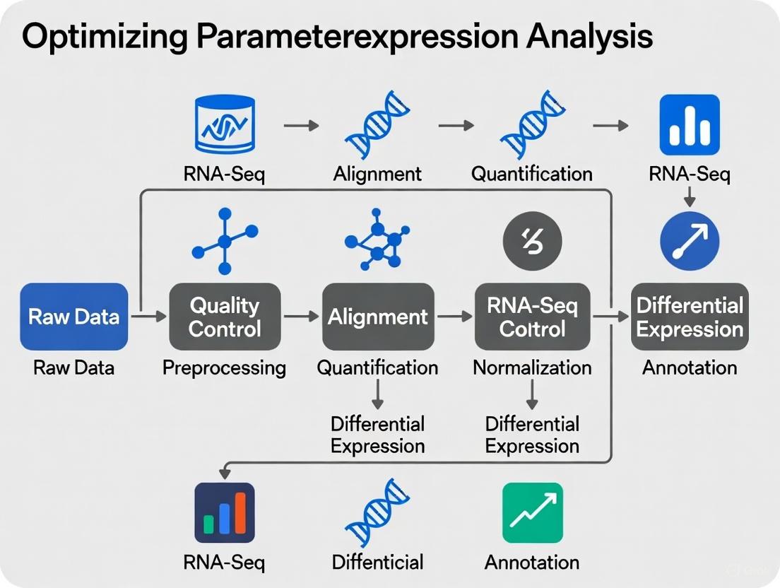
RNA-Seq Experimental Workflow
The following diagram illustrates the core steps in an RNA-Seq data analysis pipeline, from raw data to functional interpretation, including key decision points and outputs.
Normalization Techniques for Read Counts
Normalization is critical for correcting biases that make counts from different samples non-comparable. The table below summarizes common techniques.
| Method | Principle | Key Consideration |
|---|---|---|
| Total Count (TC) | Scales counts by the total number of reads (library size) in each sample. | Simple but highly sensitive to a few highly expressed genes [4]. |
| Upper Quartile (UQ) | Uses the upper quartile of counts (non-zero genes) as a scaling factor. | More robust than TC, but performance can vary [1]. |
| Median of Ratios (DESeq2) | Estimates size factors based on the median of gene-wise ratios between sample and a pseudo-reference sample. | Robust to the presence of many differentially expressed genes [7]. |
| Trimmed Mean of M (TMM) | Uses a weighted trimmed mean of the log expression ratios (M-values) between samples. | A widely used robust method, implemented in edgeR [7]. |
| Transcripts Per Million (TPM) | Normalizes for both sequencing depth and gene length. | Suitable for within-sample comparisons of transcript isoforms [5]. |
A systematic assessment of normalization methods as part of a larger pipeline comparison found that methods like TMM and those used by DESeq2 performed well in generating accurate raw gene expression signals [1].
In RNA-Sequencing (RNA-Seq) differential expression analysis, two fundamental technical uncertainties directly impact the reliability of your results: the uncertainty in read assignment (determining the genomic origin of each sequencing fragment) and the uncertainty in count estimation (quantifying gene expression levels from these assignments). These challenges are present in every RNA-Seq experiment, whether you're working with bulk or single-cell data, and they propagate through your analysis pipeline, potentially affecting downstream biological interpretations.
Read assignment uncertainty arises from factors such as ambiguous alignment of reads to multiple genomic locations, the presence of paralogous genes with similar sequences, and the challenges of accurately assigning reads to specific transcript isoforms. Count estimation uncertainty stems from technical variations in library preparation, sequencing depth, and normalization methods, which can obscure true biological differences [8] [9].
This guide addresses these challenges through practical troubleshooting advice and frequently asked questions, helping you optimize your experimental design and analytical approach for more robust differential expression results.
What is read assignment uncertainty and what causes it?
Read assignment uncertainty occurs when sequencing fragments could potentially align to multiple locations in the reference genome or be assigned to multiple genes or transcripts. This problem is particularly pronounced in several scenarios:
- Genes with paralogs or gene families: Sequence similarity between duplicated genes makes it difficult to uniquely assign reads [9]
- Alternative splicing events: Reads from shared exonic regions can belong to multiple different transcript isoforms
- Repetitive genomic regions: Areas with low-complexity sequences or transposable elements
- Incomplete genome annotation: Regions where gene boundaries or novel transcripts haven't been fully characterized
The practical consequence of this uncertainty is that some reads are "multimapped" and may be excluded from analysis or proportionally assigned, potentially skewing expression estimates for genes with homologous sequences.
What is count estimation uncertainty and what causes it?
Count estimation uncertainty refers to the technical variability in quantifying gene expression levels, even when read assignments are correct. Principal sources include:
- Library preparation biases: Systematic errors introduced during RNA extraction, amplification, or adapter ligation [8] [10]
- Sequencing depth variations: Differences in total read counts between samples affect detection sensitivity [11] [12]
- RNA composition effects: Varying proportions of RNA types between samples can skew results [13]
- GC content bias: Non-uniform amplification and sequencing efficiency based on nucleotide composition [12]
These technical variations mean that raw read counts alone do not perfectly represent true RNA abundance, necessitating appropriate normalization and statistical modeling to distinguish technical artifacts from biological signals.
Experimental Design to Minimize Uncertainty
How can I optimize my experimental design to address these uncertainties?
Strategic experimental design provides the most effective approach to mitigating technical uncertainties in RNA-Seq analysis:
Prioritize biological replication over sequencing depth: Multiple studies have demonstrated that increasing the number of biological replicates provides greater statistical power than increasing sequencing depth [11] [14] [12]. For most experiments, at least 4-6 biological replicates per condition provides a good balance between cost and statistical power [11] [14].
Utilize appropriate sequencing depth: While requirements vary by organism and research question, 20-30 million reads per sample typically provides sufficient coverage for most differential expression studies while allowing for more biological replicates within the same budget [11] [12].
Implement blocking designs: When processing large numbers of samples, distribute samples from all experimental groups across library preparation batches and sequencing lanes to avoid confounding technical and biological effects [8].
Include control RNAs or spike-ins: For specialized applications where global changes in transcript abundance are expected, spike-in RNAs can help normalize for technical variation and improve count estimation accuracy [14].
Table 1: Impact of Experimental Design Choices on Different Types of Genes
| Gene Expression Level | Recommended Biological Replicates | Recommended Library Size | Primary Uncertainty Addressed |
|---|---|---|---|
| Highly expressed genes | 4+ replicates [11] | 10-20 million reads [12] | Count estimation |
| Lowly expressed genes | 6+ replicates [11] | 20-30 million reads [11] | Both read assignment and count estimation |
| Genes with paralogs | 4+ replicates [11] | 20-30 million reads [11] | Read assignment |
What is the optimal balance between replicates and sequencing depth?
The relationship between biological replicates and sequencing depth represents a fundamental trade-off in experimental design, particularly when working with fixed budgets. Based on comprehensive power analyses:
Table 2: Power Analysis for Differential Expression Detection [11] [14] [12]
| Biological Replicates | Minimum Library Size | Expected DE Genes Detected | False Discovery Rate Control |
|---|---|---|---|
| 2-3 replicates | 20-30 million reads | ~60-70% with large effect sizes | Suboptimal (FDR > 10%) |
| 4-6 replicates | 20 million reads | ~80-90% with moderate effects | Good (FDR ~5-10%) |
| 7+ replicates | 15-20 million reads | >90% with small effects | Excellent (FDR < 5%) |
Strikingly, one study found that sequencing depth could be reduced to as low as 15% of the original depth without substantial impacts on false positive or true positive rates when sufficient biological replicates were used [12]. This highlights the critical importance of biological replication over excessive sequencing depth for differential expression analysis.
Computational Strategies to Address Uncertainty
How do I minimize read assignment uncertainty in my analysis?
Computational approaches can significantly reduce read assignment uncertainty:
Implement splice-aware aligners: Tools like STAR, HISAT2, or TopHat2 account for splice junctions when mapping reads across exon boundaries [8] [9]
Utilize transcript quantification methods: Pseudoalignment tools such as Salmon, kallisto, or RSEM can improve assignment accuracy by considering all possible transcript origins for each read [15]. These methods are particularly valuable for:
- Estimating transcript-level expression
- Correcting for changes in gene length across samples
- Handling fragments that align to multiple genes with homologous sequence [15]
Apply appropriate multimapping strategies: Rather than discussing multimapped reads, some pipelines probabilistically assign them to potential genomic origins, preserving more information from your sequencing data
Leverage comprehensive annotation: Use the most current and comprehensive annotation files for your organism, as incomplete annotation is a major source of assignment uncertainty
What normalization methods best address count estimation uncertainty?
Normalization is crucial for addressing count estimation uncertainty. The choice of method depends on your experimental context:
Trimmed Mean of M-values (TMM): Implemented in edgeR, this method assumes most genes are not differentially expressed and scales libraries based on a subset of stable genes [14] [13]
Relative Log Expression (RLE): Used in DESeq2, this method calculates scaling factors based on the geometric mean of read counts across all samples [14] [13]
Transcript-aware normalization: When using transcript quantifiers like Salmon or kallisto, the tximport package can generate offset matrices that correct for changes in effective transcript length across samples [15]
For most standard differential expression analyses, TMM and RLE normalization perform similarly well [14]. However, in experiments with global transcriptomic changes (e.g., cell differentiation), spike-in based normalization may be necessary.
Troubleshooting Common Problems
How do I diagnose and address high read assignment ambiguity?
Problem: A high percentage of reads that multimap to multiple genomic locations, leading to uncertain gene assignments.
Diagnosis Steps:
- Check alignment statistics for multimapping rates (typically reported by aligners like STAR)
- Identify whether problematic genes belong to paralogous families or repetitive regions
- Verify the quality and completeness of your reference genome annotation
Solutions:
- For genes with paralogs: Consider analyzing at the gene family level rather than individual gene level
- Implement a transcript-level analysis with tools that handle fractional read assignment [15]
- Filter out genes with consistently ambiguous assignment if they're not biologically relevant to your study
- Ensure you're using the most recent genome assembly with comprehensive annotation
How do I troubleshoot count estimation problems?
Problem: Unexpected patterns in sample clustering or high technical variation between replicates.
Diagnosis Steps:
- Examine PCA plots colored by technical factors (batch, sequencing lane) rather than biological groups
- Check for correlations between sequencing depth and variance estimates
- Verify that normalization factors are appropriately calculated and applied
Solutions:
- For batch effects: Include batch as a covariate in your statistical model [8] [15]
- For library size differences: Ensure you're using appropriate normalization methods (TMM or RLE) rather than simple library size scaling [13]
- For overdispersion: Use statistical methods like DESeq2 or edgeR that explicitly model overdispersion in count data [14] [15] [13]
- For composition biases: Consider using spike-in normalization if you have global expression changes [14]
Research Reagent Solutions
Table 3: Essential Research Reagents and Computational Tools for Addressing RNA-Seq Uncertainties
| Reagent/Tool | Type | Primary Function | Uncertainty Addressed |
|---|---|---|---|
| Spike-in RNA controls | Wet-bench reagent | Normalization for technical variation | Count estimation |
| UMI barcodes | Molecular biology | Distinguishing biological duplicates from PCR duplicates | Count estimation |
| Strand-specific library kits | Wet-bench reagent | Determining transcript strand orientation | Read assignment |
| Salmon/kallisto | Computational tool | Transcript quantification with bias correction | Both |
| DESeq2/edgeR | Computational tool | Differential expression analysis | Count estimation |
| tximport/tximeta | Computational tool | Importing transcript-level estimates | Both |
Detailed Methodologies
Protocol: Read Assignment Improvement with Pseudoalignment
Purpose: To improve read assignment accuracy using transcript-aware quantification tools.
Steps:
- Download and prepare reference transcriptome: Obtain FASTA files for your organism of interest
- Build transcriptome index: Using Salmon or kallisto's indexing function
- Quantify transcript abundances: Run quantification directly from FASTQ files (skipping alignment)
- Import to differential expression framework: Use tximport in R to create gene-level count matrices with appropriate offsets
- Proceed with standard DE analysis: Using DESeq2 or edgeR with the imported counts
Key Parameters:
- For Salmon: Use
--gcBiasand--seqBiasflags to correct for systematic biases [15] - For kallisto: Specify appropriate fragment length and standard deviation for single-end data
- For tximport: Set
countsFromAbundance = "lengthScaledTPM"for gene-level summarization
Advantages: This approach corrects for potential changes in gene length across samples, increases sensitivity by considering multimapping reads, and typically requires less computational resources than traditional alignment [15].
Protocol: Count Estimation Validation
Purpose: To validate count estimation accuracy and identify potential technical artifacts.
Steps:
- Generate diagnostic plots:
- PCA plot colored by biological and technical factors
- Sample-to-sample distance heatmap
- Distribution of log fold changes across all genes
- Check normalization factors: Verify that size factors in DESeq2 or normalization factors in edgeR are within expected ranges (typically 0.5-2.0)
- Assess dispersion estimates: Plot dispersion estimates against mean expression to ensure proper modeling
- Validate with positive controls: If available, check expression patterns of genes expected to be differentially expressed based on prior knowledge
Interpretation:
- Strong batch effects in PCA: Include batch in design formula
- Extreme normalization factors: Investigate potential sample-specific issues
- Poor dispersion fit: Consider alternative analysis methods or filtering
Frequently Asked Questions
Should I use gene-level or transcript-level analysis for my experiment?
Answer: The choice depends on your biological question and the quality of your reference annotation:
Use gene-level analysis when:
- Your primary interest is in overall gene expression changes rather than isoform usage
- Working with organisms with incomplete transcriptome annotation
- Seeking more robust and reproducible results (gene-level counts typically have less uncertainty)
Use transcript-level analysis when:
- Studying biological processes known to involve alternative splicing
- Working with well-annotated model organisms
- Willing to accept higher uncertainty in exchange for isoform-resolution insights
For most differential expression studies, gene-level analysis provides a good balance between biological insight and technical robustness. If you choose transcript-level analysis, be sure to use methods like those implemented in DESeq2 or edgeR that can handle the increased statistical uncertainty [15].
How many biological replicates do I really need for my RNA-Seq experiment?
Answer: The optimal number of replicates depends on several factors:
- For pilot studies or when expecting large effect sizes: 3-4 biological replicates per condition may be sufficient
- For standard differential expression studies: 5-6 replicates provide good power to detect moderate effect sizes while controlling false discovery rates [11] [14]
- For detecting subtle expression changes (<1.5-fold): 7+ replicates are often necessary
If you have prior RNA-Seq data from similar experiments, tools like DESeq2's estimateSizeFactors and estimateDispersions can help perform power calculations for your specific experimental context. When in doubt, err on the side of more biological replicates rather than deeper sequencing [11] [12].
What quality control metrics specifically indicate problems with read assignment or count estimation?
Answer: Key quality metrics to monitor include:
For read assignment problems:
- Low alignment rates (<70-80% of reads mapping to the reference)
- High percentages of multimapping reads (>10-20%)
- Uneven coverage across transcript bodies
- Systematic differences in these metrics between experimental groups
For count estimation problems:
- Extreme library size differences between samples (>2-fold)
- Poor correlation between technical replicates
- Batch effects visible in PCA plots that correlate with processing date rather than biology
- Abnormal distribution of fold changes (not centered around zero for null comparisons)
Most RNA-Seq analysis pipelines provide these metrics, and tools like MultiQC can help aggregate them across multiple samples for easier identification of problematic samples.
In the context of optimizing parameters for RNA-Seq differential expression analysis, the hybrid approach combining STAR alignment with Salmon quantification leverages the respective strengths of both tools. STAR provides sensitive and accurate splice-aware alignment to the genome, while Salmon uses these alignments for fast, bias-aware transcript quantification [16] [17]. This method is particularly valuable when your research aims include both novel splice junction discovery and highly accurate transcript-level expression estimates for downstream differential expression testing.
The following workflow illustrates the complete process, from raw sequencing reads to a quantified transcriptome, highlighting the integration points between STAR and Salmon.
Detailed Experimental Protocols
Protocol 1: RNA-seq Read Preprocessing and Alignment with STAR
Proper preparation of sequencing reads is a critical first step to ensure high-quality alignment and quantification [18] [19].
1. Quality Control and Trimming
- Tool: FastQC for quality control, followed by Cutadapt for trimming [18].
- Command Example:
2. Genome Alignment with STAR
- Objective: Generate a BAM file containing reads aligned to the reference genome, which will be used by Salmon.
- STAR Command Example [18]:
Protocol 2: Transcript Quantification with Salmon (Alignment-Based Mode)
This protocol uses the BAM file from STAR for transcript-level quantification.
1. Prepare Transcriptome and Decoy File
- Obtain the transcriptome sequences (FASTA) and annotation (GTF) for your organism.
- Building a decoy-aware transcriptome is recommended to reduce spurious mapping of reads from unannotated genomic loci [20] [21]. Scripts like
generateDecoyTranscriptome.shcan automate this process.
2. Run Salmon Quantification
Troubleshooting FAQs
Q1: STAR alignment produces a very small BAM file. What could be wrong?
- A: This often indicates a fundamental issue preventing successful alignment.
- Verify Reference Genome: Ensure you are using the correct genome build and version for your species.
- Check Read Files: Confirm the paths to your input FASTQ files are correct and the files are not corrupted.
- Inspect Log File: STAR generates a detailed log file. Look for error messages or warnings.
- Check Quality Metrics: Use FastQC to ensure your reads are of sufficient quality and do not originate from a different species or are heavily contaminated.
- Output Unmapped Reads: Run STAR with
--outReadsUnmapped Fastxto output the unmapped reads and investigate them further [23].
Q2: Should I use the same reference genome for both STAR and Salmon?
- A: The references are related but different.
- STAR requires a reference genome (e.g.,
genome.fa) and often a gene annotation file (GTF) to build its index. - Salmon requires a transcriptome file (e.g.,
transcripts.fa), which is a FASTA file of all known transcript sequences. This can typically be generated from the same GTF file used for STAR.
- STAR requires a reference genome (e.g.,
Q3: Why are my transcript abundance estimates from Salmon inconsistent or inaccurate?
- A: This can stem from several factors related to the input data and parameters.
- Enable ValidateMappings: Always use the
--validateMappingsflag for more accurate and sensitive mapping during quantification [20] [21]. - Use a Decoy-aware Transcriptome: This prevents mis-mapping of reads that originate from non-transcribed regions and improves accuracy [20].
- Check Library Type: Incorrectly specifying the library type (e.g., stranded vs. unstranded) with the
-lparameter is a common source of error. Use tools likeSalmon quant -l Afor auto-detection or consult your library preparation protocol [22]. - RNA Integrity: Starting with high-quality RNA (RIN > 6) is crucial, as degraded RNA can lead to 3' bias and inaccurate quantification [19].
- Enable ValidateMappings: Always use the
Q4: When is this hybrid approach particularly advantageous over using either tool alone?
- A: The hybrid approach is recommended when your analysis has dual objectives [16]. The table below summarizes the strengths of each tool and the hybrid approach.
| Tool / Approach | Primary Strength | Best For |
|---|---|---|
| STAR Alone | Sensitive alignment to the genome; novel splice junction discovery [16]. | Analyses requiring detection of novel isoforms, fusion genes, or genomic variation. |
| Salmon Alone (quasi-mapping) | Extremely fast transcript quantification directly from reads [16] [17]. | Large-scale studies where speed is critical and a well-annotated transcriptome exists. |
| STAR + Salmon (Hybrid) | Leverages STAR's alignment sensitivity and Salmon's bias-aware accurate quantification [16] [17]. | Optimal for differential expression analysis, especially when seeking a balance between novel feature discovery and quantification precision. |
The Scientist's Toolkit: Essential Research Reagents and Materials
The following table details key reagents, software, and data resources required to implement the STAR+Salmon hybrid workflow.
| Item | Function / Description | Example / Source |
|---|---|---|
| Reference Genome | Sequence of the organism's genome for read alignment. | ENSEMBL, UCSC Genome Browser, NCBI. |
| Gene Annotation (GTF/GFF) | File containing genomic coordinates of genes, transcripts, and exons. | ENSEMBL, GENCODE (for human/mouse). |
| Transcriptome (FASTA) | Sequence file of all known transcripts for quantification. | Can be generated from the GTF and genome FASTA. |
| STAR Aligner | Software for splicing-aware alignment of RNA-seq reads to the genome [18]. | https://github.com/alexdobin/STAR |
| Salmon | Software for fast, bias-aware transcript quantification from alignments or reads [20] [17]. | https://github.com/COMBINE-lab/salmon |
| FastQC | Quality control tool for high-throughput sequence data [18]. | https://www.bioinformatics.babraham.ac.uk/projects/fastqc/ |
| Cutadapt | Tool to find and remove adapter sequences, primers, and other unwanted sequences from reads [18]. | https://cutadapt.readthedocs.io/ |
| High-Quality RNA | Input biological material. Integrity is critical for success (RIN > 6 recommended) [19]. | Extracted from tissue/cells using appropriate kits. |
| Conda/Bioconda | Package manager for easy installation of bioinformatics software like Salmon and STAR [18] [22]. | https://docs.conda.io/ |
The following diagram outlines a logical decision process for troubleshooting the most common issues encountered during the alignment and quantification steps.
Troubleshooting Guides and FAQs
Biological Replicates
Q: What is the fundamental difference between biological and technical replicates? A: Biological replicates and technical replicates serve distinct purposes in experimental design:
- Biological Replicates: These are different biological specimens measured independently (e.g., three different mice from the same strain undergoing the same treatment). They account for the natural biological variation within a population [24] [25].
- Technical Replicates: These involve multiple measurements of the same biological specimen (e.g., taking the same RNA sample and processing it through three separate real-time PCR reactions). They primarily help assess measurement error or technical variability introduced by the experimental procedure itself [24] [25].
Q: Why are biological replicates considered non-negotiable in a robust RNA-Seq experimental design? A: Biological replicates are essential for several critical reasons [24] [25]:
- Estimation of Biological Variance: They allow researchers to measure the natural variation in gene expression that exists between individuals in a population. Without this, it is impossible to determine if an observed difference is due to the experimental condition or merely individual variation.
- Enhanced Statistical Power: Increasing the number of biological replicates strengthens the statistical power of differential expression analysis, making it more likely to detect true positive effects.
- Outlier Detection: They enable the identification of anomalous samples that might skew results. By calculating correlations between replicates, problematic samples can be identified and removed.
- Generalizable Conclusions: Results derived from multiple biological replicates are more likely to represent the true biological phenomenon in the broader population, rather than being an artifact of a single individual.
Q: How many biological replicates should I use for my RNA-Seq experiment? A: While more replicates are always better, practical constraints like cost must be considered. Here are the general guidelines [24] [25]:
- Minimum Recommendation: At least 3 biological replicates per condition is the widely accepted minimum for RNA-Seq experiments.
- Avoiding Two Replicates: Using only two replicates is generally discouraged. If the two results are inconsistent, there is no way to determine which one is reliable.
- Publication Standards: Experiments without biological replicates face significant challenges in publication, particularly in journals with an Impact Factor of 5 or higher.
Table 1: Recommended Number of Biological Replicates for Different Organisms
| Organism Type | Minimum Recommended Replicates | Notes on Biological Variability |
|---|---|---|
| Prokaryotes & Fungi | 3 | Generally lower individual variability, leading to higher correlation between replicates [24] |
| Plants | 3 | Moderate variability; requires strict control over growth conditions and morphology during sampling [24] |
| Animals | 3 or more | Higher individual variability; requires strict control over genetic background, age, sex, and rearing conditions [24] |
Q: Can I pool multiple biological samples into one sequencing run instead of running them as individual replicates? A: No. Pooling multiple biological samples (e.g., mixing RNA from three individuals) and sequencing them as a single sample is not a substitute for proper biological replication [24] [25]. This practice only provides an average expression value for the group and destroys all information about inter-individual variation. Consequently, you lose the ability to perform statistical tests for differential expression, and the results cannot be generalized to the population.
Q: What are the critical factors for selecting appropriate biological replicates? A: To ensure that your replicates truly measure biological variance related to your experiment, you must control for other sources of variation. The following table outlines key criteria [24] [25]:
Table 2: Sampling Requirements for High-Quality Biological Replicates
| Organism | Key Controlled Variables |
|---|---|
| Plants | Same field/plot, uniform growth, identical external morphology, same developmental stage [24] |
| Animals | Identical genetic background, same rearing conditions, same age, same sex, uniform external morphology [24] |
| Cell Cultures | Same passage number, identical culture conditions, harvested at the same confluence [25] |
Sequencing Depth and Data Analysis
Q: What are the essential steps in a standard RNA-Seq data analysis workflow? A: A typical RNA-Seq data analysis involves a series of sequential steps, from raw data to biological interpretation. The workflow can be visualized as follows:
RNA-Seq Analysis Workflow
1. Raw Data Acquisition: Download sequencing data (in SRA format) from public repositories like NCBI GEO using tools like prefetch and fasterq-dump/fastq-dump [26] [27].
2. Quality Control (QC): Assess the quality of the raw sequence files (FASTQ) using FastQC. This checks for per-base sequence quality, adapter contamination, GC content, etc. MultiQC can summarize results from multiple samples [26] [28] [27].
3. Read Trimming/Filtering: Remove low-quality bases, adapter sequences, and other artifacts using tools like fastp, Trimmomatic, or trim_galore based on the QC report [26] [28].
4. Alignment to Reference Genome: Map the high-quality reads to a reference genome using splice-aware aligners such as HISAT2 (commonly used) or STAR [26] [28] [27].
5. Quantification of Gene/Transcript Expression: Generate count matrices (the number of reads mapped to each gene) using StringTie + Ballgown or featureCounts. These raw counts are the primary input for differential expression analysis. Normalized expression values like FPKM, RPKM, or TPM can also be calculated for within-sample comparisons [26] [28].
6. Differential Expression Analysis: Identify genes that are statistically significantly expressed between conditions using specialized R/Bioconductor packages like DESeq2, edgeR, or limma [26] [28].
7. Downstream Analysis: Interpret the biological meaning of the differentially expressed genes through functional enrichment analysis (GO, KEGG) using tools like clusterProfiler or GSEA [26] [28].
Q: What are the key quantification metrics for gene expression, and how do they differ? A: Expression levels can be normalized in different ways to account for technical biases. The table below compares common metrics [29] [26]:
Table 3: Common Gene Expression Quantification Metrics in RNA-Seq
| Metric | Full Name | Formula / Principle | Primary Use |
|---|---|---|---|
| Count | - | Raw number of reads mapping to a gene/transcript. | The direct input for most statistical differential expression tools (e.g., DESeq2, edgeR). |
| CPM | Counts Per Million | (Count / Total Counts) * 10^6 | Simple normalization for total library size, useful for within-sample comparisons. Does not account for gene length. |
| FPKM | Fragments Per Kilobase of transcript per Million mapped reads | (Count / (Gene Length/1000 * Total Counts/10^6)) | Normalizes for both sequencing depth and gene length. Suitable for comparing expression of different genes within the same sample. |
| TPM | Transcripts Per Million | (Count / (Gene Length/1000)) then normalized to per million. | Similar to FPKM but with a different calculation order. Considered more stable for cross-sample comparisons [28]. |
Q: What tools and reagents are essential for a successful RNA-Seq experiment and analysis? A: The following toolkit is critical for generating and processing RNA-Seq data:
Table 4: The Scientist's Toolkit for RNA-Seq Research
| Category | Item / Software | Function / Purpose |
|---|---|---|
| Wet-Lab Reagents | RiboMinus Kit / rRNA Depletion Probes | Removal of abundant ribosomal RNA to enrich for mRNA [27]. |
| SOLiD / Illumina Library Prep Kits | Preparation of sequencing-ready libraries from RNA samples [27] [30]. | |
| QC & Preprocessing | FastQC, MultiQC | Quality control assessment of raw and processed sequencing data [26] [28]. |
| Trimmomatic, fastp | Trimming of adapter sequences and low-quality bases from reads [26] [28]. | |
| Alignment | HISAT2, STAR | Splice-aware alignment of RNA-Seq reads to a reference genome [26] [28] [27]. |
| Quantification | StringTie, featureCounts | Assembly of transcripts and generation of raw count matrices [26] [27]. |
| Differential Expression | DESeq2, edgeR, limma (R/Bioconductor) | Statistical identification of differentially expressed genes [26] [28]. |
| Functional Analysis | clusterProfiler, GSEA, DAVID | Gene Ontology (GO) and pathway (KEGG) enrichment analysis [26] [28]. |
Advanced Applications and Protocols
Q: How does single-cell RNA-Seq (scRNA-seq) differ from bulk RNA-Seq in its experimental design and application? A: Single-cell RNA sequencing (scRNA-seq) represents a major technological shift with distinct design considerations, particularly in the context of complex systems like the tumor microenvironment (TME) [31].
- Objective: While bulk RNA-seq profiles the average gene expression of a population of cells, scRNA-seq measures the transcriptome of individual cells. This allows for the dissection of cellular heterogeneity, identification of rare cell types, and characterization of novel cell states and trajectories [31].
- Application Example: In lung cancer research, scRNA-seq has been used to:
- Discover new malignant cell subpopulations (e.g., TM4SF1+/SCGB3A2+ cells) and immune cell subsets [31].
- Reveal specific cancer-associated fibroblast (CAF) subsets that correlate with poor prognosis [31].
- Analyze cell-cell communication networks using tools like CellPhoneDB and CellChat to understand mechanisms of immune suppression and therapy resistance [31].
- Design Implication: The unit of biological replication shifts from a tissue sample to an individual cell. However, technical replicates (multiple libraries from the same cell pool) and biological replicates (samples from different individuals or conditions) remain crucial for validating findings. High cell numbers (thousands per sample) are often needed to adequately capture population diversity.
Q: Can you outline a generalized experimental protocol for an RNA-Seq study? A: The following diagram and steps summarize a general protocol, adaptable from a non-model organism study [30]:
General RNA-Seq Experimental Protocol
1. Define Experimental Groups and Apply Treatment: Establish clear control and experimental groups (e.g., short-day vs. long-day photoperiod to induce diapause). Ensure adequate biological replication (n>=3 per group) from the outset [30] [32]. 2. Sample Collection and Preparation: Collect tissues or whole organisms under standardized conditions. Immediately stabilize RNA by flash-freezing in liquid nitrogen or using preservative solutions like RNAlater [30]. 3. RNA Extraction and Quality Assessment: Extract total RNA using reliable kits (e.g., phenol-chloroform based). Assess RNA integrity and purity using instruments like the Bioanalyzer; an RNA Integrity Number (RIN) > 8.0 is often recommended for high-quality libraries [30]. 4. Library Preparation and Sequencing: Use a standardized protocol, for example: - Deplete ribosomal RNA or enrich for polyadenylated mRNA. - Fragment RNA and synthesize cDNA. - Add sequencing adapters and amplify the library. - Perform quality control on the final library before sequencing on an Illumina platform (e.g., NovaSeq) to a sufficient depth (e.g., 20-40 million reads per sample for standard bulk RNA-Seq) [27] [30]. 5. Bioinformatic Analysis: Follow the workflow outlined in the previous section, from QC to differential expression and enrichment analysis [26] [28].
By adhering to these fundamental principles of experimental design—incorporating sufficient biological replicates, understanding sequencing depth needs, and following a robust analytical workflow—researchers can generate reliable, statistically sound, and biologically meaningful RNA-Seq data.
RNA sequencing (RNA-seq) is a state-of-the-art method for quantifying gene expression and performing differential expression analysis at high resolution. A number of factors influence gene quantification in RNA-seq, such as sequencing depth, gene length, RNA composition, and sample-to-sample variability [33]. Normalization is the essential process that adjusts raw transcriptomic data to account for these technical factors, ensuring that differences in normalized read counts accurately represent true biological expression rather than technical artifacts [34]. Without proper normalization, researchers risk drawing incorrect biological conclusions due to technical biases inherent in the sequencing process [35].
This guide provides a comprehensive technical resource for researchers navigating the complexities of RNA-seq normalization. Within the broader context of optimizing parameters for differential expression analysis, we compare method assumptions, applications, and limitations through structured comparisons, troubleshooting guides, and practical protocols to support robust experimental design and analysis.
Core Normalization Methods
Table 1: Core Within-Sample Normalization Methods
| Method | Full Name | Normalization Factors | Primary Use Case | Key Advantages | Key Limitations |
|---|---|---|---|---|---|
| CPM/RPM | Counts/Reads Per Million | Sequencing depth | Sequencing protocols where read count is independent of gene length [33] | Simple, intuitive calculation [36] | Does not account for gene length [36] |
| RPKM/FPKM | Reads/Fragments Per Kilobase per Million mapped reads | Gene length & sequencing depth | Within-sample comparisons in single-end (RPKM) or paired-end (FPKM) experiments [33] | Enables comparison of expression levels within a sample [34] | Not recommended for between-sample comparisons; sum of normalized counts varies between samples [33] [37] |
| TPM | Transcripts Per Million | Gene length & sequencing depth | Within-sample comparisons with improved between-sample comparability [33] | Constant sum across samples facilitates proportion-based comparisons [37] [38] | Still affected by RNA composition differences between samples [38] |
Table 2: Advanced Between-Sample Normalization Methods for Differential Expression
| Method | Full Name | Normalization Approach | Key Assumptions | Best For | Implementation |
|---|---|---|---|---|---|
| TMM | Trimmed Mean of M-values | Between-sample scaling using a reference sample [34] | Most genes are not differentially expressed [36] | Datasets with different RNA compositions or containing highly expressed genes [36] | edgeR package [39] |
| RLE/DESeq2 | Relative Log Expression | Between-sample scaling based on geometric means [39] | Most genes are not differentially expressed [36] | Datasets with substantial library size differences or where some genes are only expressed in subsets [36] | DESeq2 package [39] |
| Quantile | Quantile Normalization | Makes expression distributions identical across samples [36] | Observed distribution differences are primarily technical [36] | Complex experimental designs with multiple samples; reduces technical variation [36] | Limma-Voom package [36] |
Choosing the Right Normalization Method
The selection of an appropriate normalization method depends on your experimental design and research questions. For within-sample comparisons (comparing expression of different genes within the same sample), RPKM/FPKM or TPM are appropriate as they account for gene length differences [33] [34]. For between-sample comparisons (comparing the same gene across different samples) or differential expression analysis, more advanced between-sample normalization methods like TMM (edgeR) or RLE (DESeq2) are recommended [33] [34]. When integrating multiple datasets, batch correction methods like ComBat or Limma should be applied to remove technical artifacts introduced by different sequencing runs or facilities [34].
Troubleshooting Common Normalization Issues
Frequently Asked Questions
Why can't I directly compare RPKM/FPKM or TPM values across different samples or studies?
While RPKM/FPKM and TPM are normalized units, they represent the relative abundance of a transcript within the specific population of sequenced RNAs in each sample [38]. When sample preparation protocols or RNA populations differ significantly between samples (e.g., poly(A)+ selection vs. rRNA depletion), the proportion of gene expression is not directly comparable [38]. For example, in samples prepared with rRNA depletion, small RNAs may dominate the sequencing library, artificially deflating the TPM values of protein-coding genes compared to the same sample prepared with poly(A)+ selection [38].
What should I do when my negative controls indicate significant batch effects after normalization?
Batch effects often account for the greatest source of differential expression when combining data from multiple experiments [34]. When significant batch effects persist after standard normalization:
- Apply dedicated batch correction methods such as ComBat or Limma, which use empirical Bayes statistics to adjust for known batch variables (e.g., sequencing center, date) [34].
- Perform surrogate variable analysis (sva) to identify and estimate unknown sources of variation [34].
- Ensure proper experimental design by including technical replicates and randomizing samples across sequencing batches when possible.
How does transcriptome size variation impact single-cell RNA-seq normalization and how should I address it?
In single-cell RNA-seq, cells of different types have significantly different "true" transcriptome sizes (total mRNA molecules per cell) [40]. Standard normalization methods like CP10K (counts per 10,000) assume constant transcriptome size across all cells, which removes biological variation in total mRNA content [40]. This scaling effect causes problems when comparing different cell types or using scRNA-seq data as a reference for bulk RNA-seq deconvolution [40]. To address this, consider:
- Using specialized methods like CLTS (Count based on Linearized Transcriptome Size) that preserve transcriptome size variation [40].
- Being cautious when using CP10K-normalized scRNA-seq data as reference for bulk deconvolution, as it may lead to underestimation of rare cell type proportions [40].
What are the implications of having a large proportion of differentially expressed genes between my conditions?
Many between-sample normalization methods, including TMM and DESeq2, assume that most genes are not differentially expressed [36]. When this assumption is violated:
- TMM normalization may perform poorly as the trimming process could remove too many genes [36].
- Consider using quantile normalization or non-parametric methods that make fewer assumptions about the distribution of differentially expressed genes [36].
- Evaluate the use of spike-in controls as external standards for normalization [35].
Why am I getting different results when using the same data normalized with different methods?
Different normalization methods rely on different statistical approaches and assumptions, which can lead to varying results, particularly for low-count genes or genes with extreme expression values [41] [42]. To address this:
- Understand the assumptions of each method in relation to your data [35].
- Perform sensitivity analyses by testing multiple appropriate normalization methods and comparing consistent findings.
- Validate key results using alternative experimental approaches like qPCR for critical genes [42].
Experimental Protocols for Normalization Assessment
Protocol 1: Systematic Evaluation of Normalization Methods
This protocol is adapted from Abrams et al. (2019) for evaluating normalization efficacy in preserving biological signal while reducing technical noise [42].
Materials Needed:
- RNA-seq count matrix from a standardized dataset with known biological groups and technical replicates
- Computational environment with R/Bioconductor and appropriate normalization packages (edgeR, DESeq2, etc.)
- qPCR validation data for selected genes (optional but recommended)
Procedure:
- Data Preparation: Load your count matrix and ensure proper sample annotation including biological groups and technical batches.
- Normalization Application: Apply multiple normalization methods to your dataset (CPM, TPM, TMM, RLE, Quantile, etc.).
- Variance Decomposition: For each normalized dataset, perform ANOVA to decompose variability into:
- Biological variability (attributable to experimental conditions)
- Technical variability (attributable to sequencing site/batch)
- Residual variability (unexplained noise)
- Linearity Validation: Select genes with known linear relationships (e.g., from mixture designs) and verify that normalization preserves these expected linear relationships.
- Result Interpretation: Compare the proportion of biological variability retained by each method, prioritizing methods that maximize biological signal while minimizing residual noise.
Expected Outcomes: A successful normalization method should increase the proportion of variability attributable to biology compared to raw data while maintaining expected linear relationships between samples [42]. Based on systematic evaluations, TPM often performs well by increasing biological variability from 41% (raw) to 43% while reducing residual variability from 17% to 12% [42].
Protocol 2: Assessing Impact of Normalization on Differential Expression
This protocol evaluates how normalization choices affect differential expression results.
Materials Needed:
- RNA-seq count data from at least two biological conditions with replicates
- R/Bioconductor with edgeR, DESeq2, and limma packages
- Benchmark set of known differentially expressed genes (optional)
Procedure:
- Multiple Normalizations: Apply TMM, RLE, and TPM normalization to your count data.
- Differential Expression Analysis: Perform DE analysis using each normalized dataset with corresponding statistical methods (edgeR for TMM, DESeq2 for RLE).
- Result Comparison: Compare the lists of significantly differentially expressed genes identified by each method, noting:
- Consistency in top differentially expressed genes
- Variation in false discovery rates
- Sensitivity to outliers or highly expressed genes
- Method Validation: If available, compare results to qPCR validation data or known benchmark genes to assess accuracy.
Troubleshooting Notes: Substantial discrepancies between methods often indicate violations of methodological assumptions [35]. If results vary dramatically, investigate whether your data contains extensive global expression shifts or a high proportion of differentially expressed genes, which may require specialized normalization approaches [35].
Table 3: Essential Research Reagents and Computational Resources
| Resource Type | Specific Tool/Reagent | Primary Function | Application Context |
|---|---|---|---|
| Experimental Reagents | Oligo(dT) Magnetic Beads | Poly(A)+ RNA selection | Enriches for mRNA by selecting polyadenylated transcripts [38] |
| rRNA Depletion Kits | Removal of ribosomal RNA | Alternative to poly(A)+ selection; preserves non-polyadenylated transcripts [38] | |
| Spike-in Control RNAs | External RNA controls | Provides known quantities of exogenous transcripts for normalization quality control [35] | |
| Software Packages | edgeR (R/Bioconductor) | TMM normalization & differential expression | Implements TMM normalization for RNA-seq data [39] |
| DESeq2 (R/Bioconductor) | RLE normalization & differential expression | Implements median ratio normalization for DE analysis [39] | |
| Limma (R/Bioconductor) | Quantile normalization & linear modeling | Provides quantile normalization and batch correction methods [34] | |
| Reference Data | SEQC/MAQC-III Dataset | Standardized reference data | Large-scale benchmark dataset for normalization method evaluation [42] |
Advanced Considerations and Future Directions
As RNA-seq technologies evolve, normalization methods continue to improve. Emerging approaches include:
- Beta-Poisson Normalization: Initially designed for single-cell RNA-seq, this model-based method considers both technical noise and biological variability [36].
- SCnorm: Addresses the varying dependencies of counts on sequencing depth across different genes by estimating scale factors separately for groups of genes with similar dependence patterns [36].
- Machine Learning-Based Methods: Deep learning architectures like autoencoders show promise for learning data transformations that normalize technical variation while preserving biological information [36].
When working with specialized RNA-seq applications such as single-cell sequencing or isoform-level analysis, consult method-specific best practices and consider these emerging normalization approaches that address the unique characteristics of these data types.
Selecting Differential Expression Tools: Performance Comparisons and Best Use Cases
This technical support guide provides a comprehensive benchmarking analysis and troubleshooting resource for researchers performing differential expression (DE) analysis with RNA-Seq data. Within the broader context of optimizing parameters for RNA-Seq research, we evaluate four popular tools: DESeq2, edgeR, limma-voom, and EBSeq. Each tool employs distinct statistical approaches for addressing common challenges in RNA-Seq data, including overdispersion, small sample sizes, and varying library sizes. This guide synthesizes performance characteristics based on published studies and community experiences to help you select appropriate tools and troubleshoot common issues during experimental analysis. The FAQuantitative benchmarking reveals that proper tool selection and parameter optimization significantly impact detection power and false discovery rate control, making this guidance essential for robust differential expression analysis.
Tool Comparison & Performance Benchmarking
Statistical Foundations and Ideal Use Cases
Table 1: Core Methodologies and Performance Characteristics of DE Tools
| Aspect | DESeq2 | edgeR | limma-voom | EBSeq |
|---|---|---|---|---|
| Core Statistical Approach | Negative binomial modeling with empirical Bayes shrinkage | Negative binomial modeling with flexible dispersion estimation | Linear modeling with empirical Bayes moderation of log-CPM values | Bayesian modeling with posterior probabilities for DE |
| Default Normalization | Median ratio (RLE) | Trimmed Mean of M-values (TMM) | Weighted log-CPM transformation (voom) | GetNormalizedMat() function |
| Variance Handling | Adaptive shrinkage for dispersion and fold changes | Common, trended, or tagwise dispersion options | Precision weights unlock linear models | Models across-condition vs within-condition variability |
| Ideal Sample Size | ≥3 replicates, performs better with more [43] | ≥2 replicates, efficient with small samples [43] | ≥3 replicates per condition [43] | Not specified in results |
| Best Use Cases | Moderate to large samples, high biological variability, strong FDR control [43] | Very small sample sizes, large datasets, technical replicates [43] | Multi-factor experiments, time-series, complex designs [44] [43] | Genes with large within-condition variation [45] |
| Computational Efficiency | Can be intensive for large datasets [43] | Highly efficient, fast processing [43] | Very efficient, scales well with large datasets [43] | Not specified in results |
| Special Features | Automatic outlier detection, independent filtering, visualization tools [43] | Multiple testing strategies, quasi-likelihood options, fast exact tests [43] | Handles complex designs elegantly, integrates with other omics [44] [43] | Provides posterior probabilities for DE (PPDE), less extreme FC estimates for low expressers [45] |
Quantitative Performance Benchmarks
Table 2: Normalization and Statistical Test Performance Across Conditions
| Normalization Method | Statistical Test | Recommended Sample Size | Performance Characteristics |
|---|---|---|---|
| UQ-pgQ2 | Exact test (edgeR) | Small samples | Better power and specificity, controls false positives [46] |
| UQ-pgQ2 | QL F-test (edgeR) | Large samples (n=5,10,15) | Better type I error control in intra-group analysis [46] |
| RLE (DESeq2) | Wald test (DESeq2) | Large sample sizes | Better performance than exact test with large replicates [46] |
| TMM (edgeR) | QL F-test (edgeR) | Any sample size | Best performance across sample sizes for any normalization [46] |
| RLE/TMM/UQ | Various | Varies | Similar performance given desired sample size [46] |
Troubleshooting Guides & FAQs
Experimental Design and Setup
FAQ: How many biological replicates and what sequencing depth do I need for adequate power?
The number of biological replicates has a larger impact on detection power than library size, except for low-expressed genes where both parameters are equally important [11]. For a standard experiment, we recommend at least four biological replicates per condition and 20 million reads per sample to confidently detect approximately 1000 differentially expressed genes if they exist [11]. For studies with limited resources, edgeR performs reasonably well with only two replicates, while DESeq2 and limma-voom benefit from three or more replicates [43].
Troubleshooting Guide: No DE genes found in analysis
If your analysis returns zero differentially expressed genes despite expecting biological differences:
- Check statistical power: Ensure you have sufficient biological replicates. With small sample sizes, true differences may not reach statistical significance [47]. Consider using edgeR with its exact test or quasi-likelihood F-test for better performance with limited replicates [46] [43].
- Verify experimental design: When comparing multiple groups (e.g., before/after treatment vs. control), include all samples in a single analysis with a properly specified design matrix rather than analyzing subsets separately [47].
- Adjust significance thresholds: Relax adjusted p-value and fold change thresholds initially to check if any genes approach significance, then investigate why effect sizes might be smaller than expected.
- Confirm data integrity: Check that sample groupings and metadata are correctly specified in your analysis code.
Data Preprocessing and Quality Control
FAQ: How should I filter low-expressed genes?
Filtering low-expressed genes improves detection power by reducing multiple testing burden and focusing on biologically meaningful signals. For limma-voom, keep genes expressed in at least 80% of samples with a count per million (CPM) cutoff of 1 [44] [43]. EBSeq employs an automatic filter, excluding genes with more than 75% of values below 10 by default to ensure better model fitting [45]. You can disable this filter in EBSeq by setting Qtrm=1 and QtrmCut=0 if you need to retain low-count genes [45].
Troubleshooting Guide: Input file errors with DESeq2
When DESeq2 reports errors about "repeated input file" or "different number of rows":
- Verify replicate structure: DESeq2 and most DE tools require biological replicates and cannot run with only one sample per condition [48].
- Check feature consistency: Ensure all count files have the same number of rows (genes) in the same order. This indicates whether the same reference annotation was used for all samples [48].
- Validate upstream analysis: If counts have different numbers of features, review your alignment and quantification steps (e.g., featureCounts, HTSeq) to ensure consistency in reference annotations [48].
- Inspect data manipulation: Avoid modifying count files after generation, as this can introduce inconsistencies [48].
Tool-Specific Issues
FAQ: Why does EBSeq assign high PPDE to genes with small fold changes, and vice versa?
EBSeq calls a gene as differentially expressed (assigning high posterior probability of DE or PPDE) when across-condition variability is significantly larger than within-condition variability. A gene with large fold change might not be called DE if it also has large biological variation within conditions, as this variation could explain the across-condition difference [45]. Conversely, genes with smaller fold changes but consistent patterns across replicates may receive higher PPDE values.
FAQ: Can I use TPM/FPKM/RPKM values directly for differential expression analysis?
No, cross-sample comparisons using TPM, FPKM, or RPKM without further normalization is generally not appropriate [45]. These normalized values assume symmetric distribution of differentially expressed genes across samples, which rarely holds true in real experiments. Instead, use raw counts with library size factors or normalized counts from tool-specific functions like GetNormalizedMat() in EBSeq [45].
Troubleshooting Guide: NA values in EBSeq posterior probabilities
If your EBSeq results show "NoTest" status with NA values for posterior probabilities:
- Check default filters: EBSeq excludes genes with >75% of values <10 by default. Adjust with
Qtrm=1andQtrmCut=0parameters to disable this filter [45]. - Address numerical overflow: For genes with extremely large or small within-condition variance, numerical issues can occur. Try adjusting the
ApproxValparameter inEBTest()orEBMultiTest()(default is 10^-10) [45]. - Verify input data: Ensure count data contains appropriate variability and no extreme outliers that could cause computational issues.
Experimental Protocols & Workflows
Comprehensive RNA-Seq Analysis Workflow
Diagram 1: RNA-Seq Differential Expression Analysis Workflow
Tool Selection Decision Guide
Diagram 2: Differential Expression Tool Selection Guide
Detailed DESeq2 Protocol
Methodology for DESeq2 Analysis:
- Data Preparation: Create a count matrix with genes as rows and samples as columns, plus a metadata table with sample information.
- Create DESeq2 Object:
- Pre-filtering: Remove genes with very low counts (e.g., <10 reads across all samples).
- Specify Reference Level:
- Run DESeq Analysis:
- Extract Results:
Detailed edgeR Protocol with QL F-test
Methodology for edgeR Quasi-Likelihood Analysis:
- Create DGEList Object:
- Normalization: Calculate normalization factors using TMM method
- Filter low-expressed genes:
- Design Matrix and Dispersion Estimation:
- QL Framework:
The Scientist's Toolkit
Research Reagent Solutions
Table 3: Essential Computational Tools for RNA-Seq Analysis
| Tool Category | Specific Tools | Primary Function | Application Notes |
|---|---|---|---|
| Quality Control | FastP, TrimGalore, Trimmomatic | Adapter trimming, quality filtering | FastP offers speed and simplicity; TrimGalore provides integrated QC reports [9] |
| Alignment | STAR, HISAT2, TopHat2 | Read alignment to reference genome | STAR provides high accuracy; HISAT2 is efficient for spliced alignment [46] |
| Quantification | featureCounts, HTSeq, RSEM | Generate count matrices from aligned reads | featureCounts is fast and efficient; RSEM estimates transcript abundances [46] [9] |
| DE Analysis | DESeq2, edgeR, limma-voom, EBSeq | Identify differentially expressed genes | Choice depends on experimental design, sample size, and biological question [43] |
| Functional Analysis | GO enrichment, GSEA | Biological interpretation of DE results | Provides pathway analysis and functional annotation of results [11] |
Normalization Methods Reference
Table 4: Comparison of RNA-Seq Normalization Methods
| Normalization Method | Description | Strengths | Limitations |
|---|---|---|---|
| RLE (Relative Log Expression) | Median-based method in DESeq2 | Performs well with moderate to large sample sizes | Can be conservative with small samples [46] |
| TMM (Trimmed Mean of M-values) | Weighted trimmed mean in edgeR | Robust to highly differentially expressed genes | Can be too liberal with some data types [46] |
| Upper Quartile (UQ) | Scales using 75th percentile | Simple and intuitive | Performance varies with expression distribution [46] |
| UQ-pgQ2 | Two-step per-gene Q2 after UQ scaling | Controls false positives with small samples | Recently developed, less widely tested [46] |
| Voom Transformation | Converts counts to log-CPM with precision weights | Enables linear modeling of RNA-seq data | Requires TMM, CPM, or Upper Quartile normalization [49] |
FAQ: How does sample size impact my RNA-Seq study?
The choice of sample size, specifically the number of biological replicates per group, is one of the most critical decisions in an RNA-Seq experimental design. It directly affects the accuracy of biological variance estimation and the statistical power to detect differential expression (DE). Biological replication measures the variation within the target population and is essential for robust statistical inference that can be generalized to the entire population under study [12] [8].
- Small Sample Sizes (e.g., n=3): While n=3 is a common starting point, it often provides limited power to detect anything but the most pronounced expression differences. With only three replicates, the estimation of biological variance can be unstable, which may lead to an increased number of both false positives and false negatives unless tools with specific conservative properties are used [50].
- Larger Sample Sizes (e.g., n≥6): Increasing the number of biological replicates significantly improves the power and reliability of your study. Research has shown that power to detect DE improves markedly when the number of biological replicates is increased [12]. A study with n≥6 replicates allows for a more accurate estimation of the natural variation in gene expression, enabling the confident identification of more subtle, yet biologically important, changes [8].
Table 1: Impact of Sample Size on RNA-Seq Experimental Outcomes
| Factor | Small Samples (n=3) | Larger Samples (n≥6) |
|---|---|---|
| Biological Variance Estimation | Less accurate and stable | More accurate and reliable |
| Statistical Power | Lower; detects only large effect sizes | Higher; can detect subtler expression changes |
| False Discovery Rate (FDR) Control | More challenging; higher risk of false positives/negatives | Better controlled; more robust and trustworthy results |
| Cost Efficiency | Lower per-experiment cost, but higher risk of failed or non-reproducible studies | Higher initial cost, but much better value and reproducibility for the investment |
FAQ: Which differential expression analysis tools are best for small sample sizes (n=3)?
When working with a limited number of replicates like n=3, the primary challenge is controlling false positives due to unstable variance estimates. The choice of software is crucial to mitigate this issue.
Recommendation: For studies with n=3, DESeq (and its successor, DESeq2) is often the recommended tool. It performs more conservatively than other methods, which helps to reduce the number of false positive findings when replicate numbers are low [12] [50].
Table 2: Tool Recommendations for Small vs. Larger Sample Sizes
| Sample Size | Recommended Tools | Key Rationale | Performance Characteristics |
|---|---|---|---|
| Small (n=3) | DESeq/DESeq2 | Conservative approach, better control of false positives. | Performs more conservatively than edgeR and NBPSeq at small sample sizes [12]. |
| Larger (n≥6) | edgeR | High power to uncover true positives. | Slightly better than DESeq and Cuffdiff2 at uncovering true positives, though potentially with more false positives [50]. |
| Larger (n≥6) | Intersection of Tools | Maximizes confidence in results. | Taking the intersection of DEGs from two or more tools (e.g., DESeq & edgeR) is recommended if minimizing false positives is critical [50]. |
Decision Workflow for Tool Selection Based on Sample Size
Given budget constraints, researchers often face the decision of whether to sequence each sample more deeply or to include more biological replicates.
Strong Recommendation: The evidence strongly suggests that greater power is gained through the use of biological replicates than through increasing sequencing depth or using technical (library) replicates [12]. One study even found that sequencing depth could be reduced to as low as 15% in a multiplexed design without substantial impacts on the false positive or true positive rates, underscoring the superior value of additional biological replication [12].
Practical Protocol: Implementing a Multiplexed Design
- Library Preparation: During the library preparation step, ligate distinct indexing barcodes (short, unique DNA sequences) to the cDNA fragments of each biological sample [12].
- Pooling: Combine the individually barcoded libraries into a single pool.
- Sequencing: Sequence the pooled libraries in a single sequencing lane or reaction on a high-throughput platform (e.g., Illumina HiSeq) [12].
- Demultiplexing: After sequencing, use computational tools to allocate the generated reads back to their original samples by identifying the unique barcodes [12].
This protocol allows for the profiling of multiple samples simultaneously, dramatically reducing the cost per sample and making studies with higher biological replication (n≥6) more feasible and cost-effective [12].
Research Reagent Solutions
Table 3: Essential Materials and Tools for RNA-Seq Differential Expression Analysis
| Item Name | Function / Explanation |
|---|---|
| Barcodes/Indexes | Short DNA sequences ligated to samples for multiplexing, allowing multiple libraries to be pooled and sequenced in one lane [12]. |
| DESeq / DESeq2 | A software package for DE analysis that uses a negative binomial model and is known for its conservative performance, ideal for low-replicate studies [12] [50]. |
| edgeR | A software package for DE analysis that also uses a negative binomial model and is noted for its high power to detect true positives with sufficient replication [12] [50]. |
| Negative Binomial Model | The statistical distribution used by most modern DE tools to model RNA-Seq count data and account for technical and biological variation (overdispersion) [50]. |
| Biological Replicates | Independent samples taken from different biological units (e.g., different animals, plants, or primary cell cultures) to measure natural variation within a population [8]. |
Frequently Asked Questions
1. For a short time course experiment with only 4 time points, should I use specialized time course tools or standard pairwise comparison methods? For short time series (typically <8 time points), standard pairwise comparison approaches often outperform specialized time course tools. Research has demonstrated that classical pairwise methods show better overall performance and robustness to noise on short series, with one notable exception being ImpulseDE2. Specialized time course tools tend to produce higher numbers of false positives in these scenarios. For longer time series, however, specialized tools like splineTC and maSigPro become more efficient and generate fewer false positives [51].
2. What is the fundamental statistical reason for choosing pairwise methods over temporal tools for short series? Specialized time course tools must account for temporal dependencies between time points, which requires estimating more complex statistical models with additional parameters. With limited time points (short series), these models can be underpowered and overfit the data, leading to increased false positives. Pairwise methods, building separate models for each comparison, have a simpler statistical structure that is more robust with limited data points [51] [52].
3. How does the number of biological replicates impact my choice of analysis method for time course data? The number of biological replicates significantly influences analysis power more than sequencing depth. For time course experiments, sufficient replicates are crucial for both pairwise and specialized temporal methods to accurately capture biological variation. When resources are limited, prioritizing more replicates over deeper sequencing or more time points generally provides better detection power for differentially expressed genes [11] [53] [54].
4. Can I use standard RNA-seq tools like DESeq2 or edgeR for time course experiments? Yes, both DESeq2 and edgeR can be applied to time course data. These tools can perform pairwise comparisons between individual time points or to a reference time point (typically time zero). They can also model time as a continuous variable in generalized linear models to test for expression trends over time. These packages use negative binomial distributions to model count data, which appropriately handles biological variation [55] [56] [46].
Troubleshooting Guides
Problem: High False Positive Rates in Short Time Course Analysis
Issue: Your time course analysis with limited time points is identifying many potentially false positive differentially expressed genes.
Solution:
- Apply pairwise methods: Use DESeq2 or edgeR to perform comparisons between individual time points or each time point against the baseline instead of specialized temporal tools [51].
- Overlap candidate lists: When using multiple analysis methods, consider taking the intersection of genes identified by different tools, as true positives are more likely to overlap while false positives tend to be method-specific [51].
- Adjust filtering thresholds: Implement more stringent false discovery rate (FDR) controls. Research suggests using approximately 2⁻ʳ as an FDR threshold, where r is your replicate number [54].
Table 1: Method Recommendations Based on Time Series Characteristics
| Series Length | Recommended Approach | Key Tools | Performance Notes |
|---|---|---|---|
| Short (<8 time points) | Pairwise comparisons | DESeq2, edgeR, ImpulseDE2 | Better overall performance, fewer false positives [51] |
| Long (≥8 time points) | Specialized temporal methods | splineTC, maSigPro | More efficient, identifies fewer false positives [51] |
| Any length with limited replicates | Pairwise approaches | DESeq2, edgeR | More robust with limited replication [51] [46] |
Problem: Choosing Between Normalization Methods for Time Course Data
Issue: Uncertainty about which normalization method is most appropriate for time course RNA-seq data.
Solution:
- Standard approaches: Use relative log expression (RLE) normalization (DESeq2) or trimmed mean of M-values (TMM) normalization (edgeR) for most time course experiments [55] [46].
- Complex designs: For data with substantial technical variability or batch effects, consider using the UQ-pgQ2 normalization method, particularly when combined with exact tests or quasi-likelihood F-tests [46].
- Consistency check: Perform principal component analysis (PCA) on normalized data to verify that samples cluster by biological factors rather than technical batches [55].
Problem: Inadequate Experimental Design for Temporal Analysis
Issue: The experimental design may not support robust detection of temporal expression patterns.
Solution:
- Increase replication: Prioritize biological replicates over sequencing depth. Studies show that power increases significantly with more replicates, with 4-6 replicates per time point providing substantially better detection than 2-3 replicates [11] [54].
- Balance time and replication: With limited resources, consider reducing the number of time points in favor of more replicates at each remaining time point for short series [51].
- Validate with positive controls: Include known positive control genes or spike-in standards when possible to verify detection sensitivity [46].
Table 2: Essential Research Reagent Solutions for RNA-Seq Time Course Experiments
| Reagent/Category | Function/Purpose | Implementation Considerations |
|---|---|---|
| Biological Replicates | Account for biological variation | Minimum 4 replicates per time point; 6+ for better power [11] [54] |
| rRNA Depletion Kits | Remove ribosomal RNA | Essential for non-polyA transcripts; improves transcriptome coverage |
| mRNA Enrichment Kits | Select polyadenylated RNA | Standard for mRNA sequencing; may miss non-polyA transcripts |
| UMIs (Unique Molecular Identifiers) | Correct for PCR amplification biases | Essential for accurate transcript quantification; reduces technical noise |
| Spike-in RNA Controls | Normalization and QC | Added to each sample; monitors technical variability across samples [46] |
| Library Preparation Kits | Convert RNA to sequence-ready libraries | Consider compatibility with your sequencing platform |
Experimental Protocol: Comparative Analysis of Methods
Methodology for Evaluating Analysis Approaches
When designing a time course experiment, consider running parallel analyses with both pairwise and specialized temporal methods to evaluate their performance on your specific data.
Input Data Requirements:
- Count matrix: Raw read counts per gene across all samples (output from HTSeq, featureCounts, etc.) [53]
- Experimental design matrix: Sample information including time points, replicates, and conditions [55]
- Quality metrics: Sequencing depth, mapping rates, and sample-level QC statistics [56]
Analysis Workflow:
- Quality Control: Assess read distribution, outlier samples, and batch effects
- Normalization: Apply appropriate normalization (RLE, TMM, or UQ-pgQ2) based on data characteristics [46]
- Parallel Analysis:
- Run pairwise comparisons (e.g., DESeq2, edgeR) comparing each time point to baseline
- Run specialized temporal methods (e.g., splineTC, maSigPro, ImpulseDE2)
- Result Integration: Compare identified gene lists, focusing on overlapping candidates
- Validation: Select candidates for experimental validation, prioritizing genes identified by multiple methods
Key Decision Factors
When choosing between analysis approaches for your time course data, consider these critical factors:
- Series Length: Short series (<8 time points) generally favor pairwise methods [51]
- Replication Level: Limited replication (<3 per time point) increases value of simpler pairwise approaches [11]
- Biological Question: Are you interested in specific time point comparisons or overall temporal trends?
- Computational Resources: Specialized temporal methods often require more computational power and memory
- Expected Patterns: Simple monotonic trends versus complex oscillatory or multiphasic expression patterns
The optimal approach depends on your specific experimental context, and in many cases, running multiple analysis methods provides the most comprehensive insights into your temporal gene expression data.
Frequently Asked Questions
Q1: Which distribution should I choose for a standard RNA-Seq differential expression analysis? For most use cases, the Negative Binomial (NB) distribution is recommended. It is specifically designed to model count-based sequencing data and explicitly accounts for overdispersion (variance greater than the mean), a common characteristic of RNA-Seq data [57] [55]. Popular and widely validated tools like DESeq2 and edgeR are built upon the NB framework [57] [58].
Q2: My sample size is very small (e.g., n=3 per group). Is the Negative Binomial still appropriate? Yes, but the choice of method is crucial. One evaluation study found that with a sample size of 3 per group, EBSeq performed better in terms of false discovery rate (FDR) control and power. For sample sizes of 6 or 12 per group, DESeq2 is recommended [57]. Note that for very small samples, the per-gene dispersion estimates for the NB model are unreliable, and methods that "shrink" dispersion estimates by borrowing information across genes are essential [58].
Q3: When would I consider using a log-normal distribution? The log-normal distribution can be a good choice when the relationship between a continuous covariate (e.g., age, disease severity score) and gene expression is suspected to be nonlinear [59]. Empirical studies of real gene expression profiles have also found that a significant portion (around 80%) of gene expression profiles follow normal or log-normal distributions [60]. If your data is log-normally distributed, both DESeq and DESeq2 have been shown to perform well [57].
Q4: How can I check if my data fits a Negative Binomial distribution?
Formal statistical tests exist, but it is important to know that real RNA-Seq data does not always perfectly fit the NB model. One study that applied a goodness-of-fit test found that the NB assumption was violated in many public datasets [61]. This can lead to poor false discovery rate control. If you suspect a poor fit, consider using non-parametric methods like SAMSeq or compositionally aware tools like ALDEx2 as a complementary analysis [62] [61].
Q5: What is the impact of normalization on the data distribution? Normalization is a critical pre-processing step that places expression data from all samples into the same distribution, removing technical variations like sequencing depth and RNA composition [55]. The choice of normalization method can significantly impact your results. Methods like DESeq's median-of-ratios and edgeR's TMM are designed for count data and are robust [63] [55]. Some common normalization methods like Total Count or Quantile normalization have been shown to perform poorly in comparative studies [63].
Troubleshooting Guides
Issue 1: Poor Model Fit or Inflated False Discoveries
Symptoms: Your differential expression analysis returns an unexpectedly high number of significant genes, or the p-value distribution looks unusual. Validation experiments fail to confirm your top hits.
Possible Causes and Solutions:
Cause: Violation of distributional assumptions. Your data may not conform to the distribution (e.g., Negative Binomial) assumed by your chosen tool.
- Solution A: Conduct a goodness-of-fit test for the Negative Binomial distribution, as described in [61].
- Solution B: Switch to or compare results with a non-parametric method.
SAMSeqis a non-parametric method that can be more robust when distributional assumptions are violated [57] [61].ALDEx2, which uses a log-ratio transformation, is another alternative known for high precision [62].
Cause: Inaccurate dispersion estimation in small sample studies.
- Solution: Use tools that employ shrinkage estimators for dispersion. DESeq2 and edgeR use empirical Bayes methods to stabilize dispersion estimates across genes, which is vital for experiments with low replication [57] [58]. The
sSeqpackage was also specifically proposed for improved dispersion estimation in small sample sizes [58].
- Solution: Use tools that employ shrinkage estimators for dispersion. DESeq2 and edgeR use empirical Bayes methods to stabilize dispersion estimates across genes, which is vital for experiments with low replication [57] [58]. The
Issue 2: Handling Nonlinear Relationships with Covariates
Symptoms: You have a continuous predictor variable (e.g., patient age, drug dosage, time series) and visual inspection suggests a curved, not straight-line, relationship with gene expression.
Possible Cause and Solution:
- Cause: Standard Generalized Linear Models (GLMs) in tools like DESeq2 assume a linear relationship on the log scale.
- Solution: Use a method that can fit generalized additive models (GAMs). The
NBAMSeqpackage extends the Negative Binomial model to include nonlinear smooth functions of covariates, allowing it to capture complex relationships that a linear model would miss [59].
- Solution: Use a method that can fit generalized additive models (GAMs). The
Performance Comparison and Decision Workflow
The table below summarizes key characteristics of the two distributions based on empirical evaluations.
Table 1: Empirical Performance of Data Distributions in RNA-Seq Analysis
| Distribution | Recommended Sample Size | Recommended Tools | Strengths | Weaknesses/Limitations |
|---|---|---|---|---|
| Negative Binomial | • n ≥ 6: DESeq2 [57]• n = 3: EBSeq [57] | DESeq2, edgeR, EBSeq, baySeq, sSeq [57] [58] | • Directly models count data [55].• Explicitly accounts for overdispersion [57].• Widely adopted and validated. | • Poor FDR control if assumption is violated [61].• Unreliable gene-specific dispersion estimates with small n [58]. |
| Log-Normal | All sample sizes (when data is log-normal) [57] | DESeq, DESeq2, VOOM (limma) [57] [59] | • Can be robust [63].• Suitable when data is truly log-normal [60].• VOOM is effective for complex designs. | • May not properly handle the mean-variance relationship of counts [57]. |
The following workflow diagram integrates this information to guide your decision-making process.
Experimental Protocols for Performance Evaluation
Protocol 1: Benchmarking Distributional Fit and Differential Expression Performance
This protocol is adapted from methodologies used in several comparative studies [57] [61] [60].
Objective: To systematically evaluate whether a Negative Binomial or log-normal-based model is more appropriate for a given RNA-Seq dataset and to assess the performance of different tools.
Materials:
- RNA-Seq Count Matrix: A table where rows are genes/transcripts and columns are samples.
- Phenotype Data: A file describing the experimental conditions or covariates for each sample.
- Software: R/Bioconductor environment.
Methodology:
Data Pre-processing:
- Filtering: Remove genes with very low counts across all samples. A common strategy is to remove genes that do not have a minimum count (e.g., 5-10 reads) in a minimum number of samples (e.g., the size of the smallest group) [63] [55].
- Normalization: Account for differences in library size and RNA composition. For NB-based methods, use the built-in normalization (e.g., DESeq2's "median-of-ratios" [55] or edgeR's "TMM" [63]).
Goodness-of-Fit Testing:
- Formally test the fit of the Negative Binomial distribution for each gene using a dedicated goodness-of-fit test, such as the smooth test described in [61].
- Visually inspect the mean-variance relationship in your data. A plot of the variance against the mean should be consistent with the quadratic mean-variance relationship assumed by the NB model [55].
Differential Expression Analysis:
- Analyze the same dataset with multiple methods representing different distributional assumptions. For example:
- NB-based: DESeq2, edgeR
- Log-normal/Linear Model-based: VOOM (limma)
- Non-parametric: SAMSeq
- Compositional Log-ratio: ALDEx2
- Analyze the same dataset with multiple methods representing different distributional assumptions. For example:
Performance Metrics:
- Concordance: Examine the overlap in the lists of significantly differentially expressed genes identified by the different methods.
- False Discovery Rate (FDR) Control: If a "ground truth" is available (e.g., via simulation or spike-in controls like ERCCs), evaluate which methods best control the FDR at the nominal level [57] [61].
- Power (Sensitivity): Assess the number of true positives detected by each method.
The Scientist's Toolkit: Essential Research Reagents & Software
Table 2: Key Tools and Resources for RNA-Seq Distribution Analysis
| Item Name | Type | Primary Function | Key Consideration |
|---|---|---|---|
| DESeq2 [57] [55] | R/Bioconductor Package | Differential expression analysis using a Negative Binomial GLM with shrinkage estimators. | Recommended for sample sizes ≥ 6. Robust and highly cited. |
| edgeR [57] [58] | R/Bioconductor Package | Differential expression analysis using a Negative Binomial model with empirical Bayes dispersion estimation. | Flexible, good for complex experimental designs. |
| EBSeq [57] | R/Bioconductor Package | Differential expression analysis using a Bayesian hierarchical NB model. | Particularly recommended for studies with very small sample sizes (n=3). |
| NBAMSeq [59] | R/Bioconductor Package | Negative Binomial Additive Model. Captures nonlinear effects of continuous covariates. | Use when you suspect a nonlinear relationship between a covariate and expression. |
| ALDEx2 [62] | R/Bioconductor Package | Differential abundance analysis using compositional data analysis and log-ratio transformations. | High precision; useful when NB assumption is violated; works on multiple data types. |
| SAMSeq [57] [61] | R Package | Non-parametric differential expression analysis based on the Wilcoxon rank statistic. | Robust choice when distributional assumptions are in doubt. |
| sSeq [58] | R Package | Differential expression analysis with a simple, effective shrinkage estimator for dispersion. | Designed for improved performance in experiments with small sample size. |
Single-cell RNA sequencing (scRNA-seq) has revolutionized biological research by enabling the profiling of gene expression at the individual cell level, revealing unprecedented insights into cellular heterogeneity [64]. Unlike bulk RNA-seq, which provides averaged expression profiles across cell populations, scRNA-seq can identify rare cell types, transitional states, and the full spectrum of cellular diversity within tissues [64] [65]. However, this technology faces significant technical challenges, primarily dropout events and data heterogeneity, which complicate downstream analysis and biological interpretation [66] [67].
Dropout events refer to the phenomenon where expressed genes in individual cells show zero counts due to technical limitations rather than true biological absence [66] [65]. These events arise from the extremely low starting amounts of mRNA in individual cells and inefficiencies in reverse transcription, amplification, and library preparation [64]. The resulting data sparsity can obscure true biological signals, complicate cell type identification, and reduce statistical power for detecting differentially expressed genes [67]. Simultaneously, scRNA-seq data exhibits multiple sources of heterogeneity—both biological, reflecting true cellular diversity, and technical, arising from experimental variability [68]. Addressing these intertwined challenges requires specialized computational and experimental approaches throughout the entire workflow, from study design to data interpretation.
Methodological Approaches for Dropout Imputation
Computational Frameworks and Algorithms
Multiple computational strategies have been developed to address dropout events in scRNA-seq data, each with distinct theoretical foundations and implementation approaches.
Consensus clustering-based methods like CCI (Consensus Clustering-based Imputation) perform clustering on multiple gene subset samples to define cellular similarities, then leverage information from similar cells to impute gene expression values [66]. This approach demonstrates particular strength in preserving data patterns while improving downstream analytical performance across diverse scenarios [66].
Deep learning-embedded statistical frameworks represent a more recent advancement. ZILLNB integrates zero-inflated negative binomial (ZINB) regression with deep generative modeling, employing an ensemble architecture that combines Information Variational Autoencoder (InfoVAE) and Generative Adversarial Network (GAN) to learn latent representations at cellular and gene levels [68]. These latent factors serve as dynamic covariates within the ZINB regression framework, with parameters iteratively optimized through an Expectation-Maximization algorithm [68]. This hybrid approach enables systematic decomposition of technical variability from intrinsic biological heterogeneity.
Denoising autoencoders with contrastive learning, exemplified by DropDAE, represent another innovative approach. This method corrupts input data by artificially introducing additional dropout events, then trains an autoencoder to reconstruct the original data while incorporating contrastive learning to enhance cluster separation in the latent space [65]. The model's loss function combines mean squared error (for reconstruction accuracy) with triplet loss (for cluster separation), effectively balancing denoising performance with improved cell type identification [65].
Performance Comparison of Imputation Methods
Table 1: Comparative Performance of scRNA-seq Imputation Methods
| Method | Underlying Approach | Key Advantages | Reported Performance Gains |
|---|---|---|---|
| CCI | Consensus clustering | Robust across different scenarios; improves downstream analyses | Comprehensive evaluations show accuracy and generalization [66] |
| ZILLNB | ZINB regression + deep learning (InfoVAE-GAN) | Decomposes technical and biological variability; handles multiple noise sources | ARI/AMI improvements of 0.05-0.2 over existing methods; AUC improvements of 0.05-0.3 for differential expression [68] |
| DropDAE | Denoising autoencoder + contrastive learning | Enhances cluster separation; avoids parametric assumptions | Outperforms existing methods in accuracy and robustness in multiple simulation settings [65] |
| Traditional Statistical Methods (scImpute, VIPER, SAVER, ALRA) | Statistical modeling | Maintain interpretability; explicit probabilistic frameworks | Limited capacity for capturing complex non-linear relationships [68] |
| Deep Learning Methods (DCA, DeepImpute, scMultiGAN) | Neural networks (autoencoders, GANs) | Capture complex nonlinear relationships; scalability | Prone to overfitting; lack mechanistic interpretability [68] |
Troubleshooting Guide: FAQs on Dropout Challenges
Experimental Design and Optimization
Q: What experimental strategies can minimize dropout events during single-cell isolation and library preparation?
A: Several experimental optimizations can significantly reduce dropout rates:
- Pilot experiments are crucial for optimizing conditions with different sample types, helping identify issues before large-scale experiments [69]. Controls should include positive controls with RNA input mass similar to your experimental samples and negative controls treated the same as actual samples.
- Appropriate cell suspension buffers are critical—resuspend cells in EDTA-, Mg2+-, and Ca2+-free 1X PBS to avoid interference with reverse transcription reactions [69]. When using FACS sorting, collect cells into freshly prepared lysis buffer containing RNase inhibitor [69].
- Minimize processing time between cell collection, snap-freezing, and cDNA synthesis to reduce RNA degradation [69]. Work quickly and maintain consistent handling throughout the protocol.
- Practice strict RNA-seq techniques: Use clean lab coats, sleeve covers, gloves changed between steps, and separate pre- and post-PCR workspaces to prevent contamination [69]. Use RNase- and DNase-free, low-binding plasticware to minimize sample loss.
Q: How can researchers optimize scRNA-seq protocols for sensitive cell types like stem cells?
A: Working with sensitive cells like hematopoietic stem/progenitor cells (HSPCs) requires additional considerations:
- Implement careful sorting strategies using surface markers to enrich target populations. For HSPCs, this includes antibodies against CD34 and/or CD133 and CD45 antigens, with depletion of cells expressing lineage differentiation markers [70].
- Adjust quality control thresholds appropriately—for HSPC analysis, cells with fewer than 200 transcripts or more than 2,500 transcripts were excluded, along with those containing >5% mitochondrial transcripts [70].
- Use integrated analysis approaches for similar cell populations—CD34+ and CD133+ HSPCs can be merged and treated as "pseudobulk" for certain analyses despite surface marker differences [70].
Computational Analysis and Quality Control
Q: What quality control metrics specifically help identify dropout-affected datasets?
A: Three key QC covariates should be examined jointly:
- Count depth: The number of counts per barcode, with unexpectedly low counts potentially indicating dying cells or technical issues [71].
- Genes per barcode: The number of detected genes per cell, with low numbers suggesting poor cell quality or technical dropouts [71].
- Mitochondrial fraction: The fraction of counts from mitochondrial genes, with high fractions indicating broken cell membranes where cytoplasmic mRNA has leaked out [71]. These metrics should be examined together rather than in isolation, as each has biological interpretations that could be misinterpreted if considered alone [71].
Q: What computational approaches best address dropout events while preserving biological heterogeneity?
A: The optimal approach depends on your data characteristics and research goals:
- For interpretability: Statistical approaches like ZILLNB provide a principled framework that integrates statistical modeling with deep learning, offering robust performance across diverse analytical tasks while maintaining some interpretability [68].
- For clustering performance: Methods incorporating contrastive learning like DropDAE specifically enhance cluster separation while addressing dropouts, making them ideal for cell type identification [65].
- For general robustness: Consensus-based methods like CCI demonstrate strong performance across different scenarios and good generalization capabilities [66]. Regardless of method, always validate imputation results using biological knowledge and compare multiple approaches when possible.
Essential Research Reagent Solutions
Table 2: Key Research Reagents for scRNA-seq Experiments
| Reagent/Kit | Primary Function | Application Notes |
|---|---|---|
| SMART-Seq v4 | Single-cell RNA-seq library prep | Recommended FACS collection: 11.5 µl 1X Reaction Buffer; Alternative: <5 µl Mg2+- and Ca2+-free 1X PBS [69] |
| SMART-Seq HT | High-throughput scRNA-seq | Recommended FACS collection: 12.5 µl CDS Sorting Solution; Alternatives: 11.5 µl Plain Sorting Solution or <5 µl Mg2+- and Ca2+-free 1X PBS [69] |
| SMART-Seq Stranded | Strand-specific scRNA-seq | Recommended FACS collection: 7 µl Mg2+- and Ca2+-free 1X PBS; Alternative: 8 µl 1.25X Lysis Buffer Mix [69] |
| Chromium Next GEM Chip G | Single-cell partitioning | Enables single-cell isolation and barcoding for 10X Genomics platform [70] |
| Chromium Next GEM Single Cell 3' Kit | Library preparation | Used for GEM generation, barcoding, and library construction in droplet-based systems [70] |
| Ficoll-Paque | Mononuclear cell separation | Enables isolation of mononuclear cells from heterogeneous tissue samples like umbilical cord blood [70] |
Integrated Workflow for Addressing Dropouts and Heterogeneity
Successfully addressing dropout events and heterogeneity requires an integrated approach spanning experimental and computational phases. The following workflow visualization illustrates the critical decision points and their relationships in optimizing scRNA-seq analyses:
Diagram 1: Integrated workflow for addressing scRNA-seq dropouts and heterogeneity, showing critical decision points from experimental design through biological validation.
Methodological Relationships and Applications
Understanding how different methodological approaches interrelate and complement each other is essential for selecting appropriate strategies. The following diagram maps the methodological landscape for addressing scRNA-seq data challenges:
Diagram 2: Methodological landscape showing relationships between experimental and computational approaches for addressing scRNA-seq data challenges.
Addressing dropout events and data heterogeneity in scRNA-seq requires a multifaceted approach combining rigorous experimental design with sophisticated computational methods. Experimental optimizations—including pilot studies, proper buffer conditions, and strict RNA-seq techniques—form the foundation for reducing technical artifacts [69]. Computational advancements in imputation methods, particularly hybrid frameworks like ZILLNB that integrate statistical modeling with deep learning, and cluster-enhanced approaches like DropDAE and CCI, offer powerful solutions for recovering biological signals from sparse data [66] [68] [65].
Future methodological developments will likely focus on better integration of multi-omics data at single-cell resolution, improved handling of rare cell populations, and more interpretable deep learning models that provide biological insights beyond imputation accuracy. As these technologies mature, standardized workflows incorporating current best practices will enable more reliable biological discoveries across diverse applications, from basic developmental biology to clinical translational research [72] [71]. By systematically addressing both technical and analytical challenges, researchers can fully leverage the potential of scRNA-seq to unravel cellular heterogeneity in health and disease.
Addressing Common Pitfalls: Batch Effects, Normalization Challenges, and False Discoveries
Core Concepts and Importance
What is technical variation in RNA-Seq data and why does it matter?
Technical variation in RNA-Seq data refers to non-biological fluctuations in gene expression measurements arising from experimental procedures rather than the biological conditions under study. This includes batch effects, library preparation differences, sequencing lane effects, and other technical artifacts. In differential expression analysis, failing to account for these hidden factors can substantially confound results, leading to both false positives and false negatives [73] [74]. Managing this variation is particularly crucial for drug development research where accurate identification of differentially expressed genes can influence downstream validation experiments and therapeutic target selection.
How do hidden factors differ from measured covariates?
Measured covariates are known sample characteristics (e.g., age, sex, treatment group) that researchers explicitly record during experimental design. In contrast, hidden factors are unmeasured or unanticipated variables that systematically influence gene expression patterns. These hidden factors can correlate with your primary variable of interest, potentially obscuring true biological signals if not properly addressed [73] [74]. Surrogate Variable Analysis (SVA) specifically addresses this challenge by estimating these hidden factors directly from the gene expression data itself.
Adjustment Strategies and Performance
What methods are available for managing technical variation?
Two primary integrated strategies combine covariate selection with hidden factor adjustment:
- FSR_sva: First uses the False Selection Rate (FSR) method to identify relevant measured covariates, then estimates surrogate variables based on these selected covariates [73]
- SVAall_FSR: First estimates surrogate variables using all available covariates, then applies FSR selection to the combined set of original covariates and surrogate variables [73]
When should I choose each method?
The optimal strategy depends on your specific experimental context and the relationship between your measured covariates and primary factor of interest:
| Method | Best Use Case | Performance Characteristics |
|---|---|---|
| FSR_sva | When no available relevant covariates are strongly associated with the main factor of interest | Performs comparably to existing methods in this scenario [73] |
| SVAall_FSR | When some available relevant covariates are strongly correlated with the primary factor of interest | Achieves the best performance among compared methods in this situation [73] |
For single-cell RNA-Seq data where multiple correlated hidden sources exist, IA-SVA (Iteratively Adjusted SVA) is particularly effective as it can estimate hidden factors even when they are correlated with known factors, unlike traditional SVA methods that enforce orthogonality [74].
How effective are these methods in practice?
Simulation studies demonstrate that IA-SVA provides equal or better detection power and estimation accuracy compared to traditional SVA methods while properly controlling Type I error rates (0.04 for IA-SVA versus 0.09 for USVA and SSVA) [74]. IA-SVA shows particular advantages when hidden factors affect a small percentage of genes and when factors are correlated with known variables.
The following workflow illustrates the two main strategies for integrating covariate selection with hidden factor adjustment:
Experimental Protocols
How do I implement the FSR method for covariate selection?
The FSR (False Selection Rate) variable selection method extends the approach of Wu et al. to multi-response settings for RNA-Seq data [73]. Implementation involves these steps:
- Preprocessing: Transform raw counts to log-counts per million using the voom procedure with library sizes computed as the 75th percentile of sample counts [73]
- Model Fitting: For each candidate model containing a subset of covariates, fit linear models for all genes
- Precision Weights: Compute precision weights via LOWESS regression of residual standard deviations on mean log-counts
- Relevance Measurement: For each covariate j, calculate relevance measure r(pj) = ΣI(pgj ≤ 0.05)/max(ΣI(pgj ≥ 0.75)/5, 1) where I is the indicator function
- Backward Selection: Apply backward selection controlling the expected proportion of irrelevant covariates selected at target level α0
This method is implemented in the FSRAnalysisBS function of the R package csrnaseq [73].
What is the complete SVA workflow?
The standard SVA workflow can be implemented using the sva function in the R package sva (version 3.56.0) for log-transformed RNA-seq count data [73]. For enhanced performance with correlated factors:
- Initialization: Use the
ia.svafunction to initialize the algorithm - Iterative Adjustment: Apply
ia.svaiteratively until all significant surrogate variables are identified - Significance Testing: Assess significance of each detected factor using permutation testing
- Gene Identification: Obtain sets of genes associated with each significant hidden factor
- Downstream Analysis: Include significant surrogate variables as covariates in differential expression analysis
IA-SVA specifically improves upon traditional SVA by identifying hidden factors correlated with known factors and providing gene sets associated with each detected hidden source [74].
Troubleshooting Common Issues
How can I diagnose hidden variation in my dataset?
Several quality control approaches can help identify potential hidden variation:
- Principal Component Analysis (PCA): Plot samples in PCA space and color by potential batch variables to identify patterns
- Hierarchical Clustering: Check if samples cluster by technical factors rather than biological groups
- Statistical Tests: Use the
ia.svafunction with permutation testing to statistically assess the presence of hidden factors - Control Genes: Examine expression patterns of known housekeeping genes across samples
Unexplained patterns in these diagnostics suggest potential hidden factors that should be addressed.
What if my hidden factors correlate with my primary variable?
When hidden factors correlate with your primary variable of interest, standard SVA methods that enforce orthogonality may produce biased results. In this case:
- Use IA-SVA which specifically handles correlated factors without the orthogonality constraint [74]
- Consider the SVAall_FSR approach which performs better when covariates are strongly correlated with the primary factor [73]
- Validate findings with orthogonal experimental approaches when possible
Simulation studies show IA-SVA maintains accurate estimation (correlation >0.95 with true factors) even when factors are moderately correlated (|r| = 0.3-0.6) with known variables [74].
How do I validate that my adjustment worked properly?
Post-adjustment validation should include:
- PCA Examination: Confirm that technical patterns are reduced while biological signal remains
- Positive Control Verification: Ensure known biologically relevant genes remain significant
- Negative Control Check: Verify that established non-differentially expressed genes show minimal changes
- Simulation Testing: Compare results with simulated data where ground truth is known
- Biological Consistency: Assess whether results align with established biological knowledge
Essential Research Reagent Solutions
What computational tools are essential for implementing these methods?
| Tool/Resource | Function | Implementation |
|---|---|---|
| csrnaseq R package | FSR-controlled variable selection | FSRAnalysisBS function [73] |
| sva R package (v3.56.0+) | Surrogate Variable Analysis | sva function for log-transformed counts [73] |
| IA-SVA | Handling correlated hidden factors | ia.sva function for single-cell and bulk data [74] |
| voom/limma | Precision weights and differential expression | Transformation and moderated testing [73] |
| FastQC | Raw read quality control | Initial quality assessment [75] [9] |
| Trim Galore/fastp | Read trimming and adapter removal | Data preprocessing [9] |
In RNA sequencing (RNA-Seq) analysis, normalization is not an optional preprocessing step but a critical statistical procedure that directly controls data interpretation and the validity of scientific conclusions. The "Scale Problem" refers to the fundamental challenge that raw read counts from RNA-Seq experiments are influenced by multiple technical factors unrelated to biological expression, particularly sequencing depth (the total number of reads generated per sample) [76] [35]. Without proper normalization, genes appearing differentially expressed might simply reflect these technical variations, leading to compromised analyses.
This technical guide addresses how implicit assumptions embedded within normalization methods directly impact False Discovery Rate (FDR) control. When normalization assumptions align with experimental conditions, statistical tests perform optimally, correctly identifying truly differentially expressed genes. However, when these assumptions are violated—such as in experiments with global transcriptional shifts or extreme expression changes in few genes—the result is inflated FDRs and potentially irreproducible biological conclusions [35] [77]. Understanding these relationships is essential for optimizing differential expression analysis parameters and ensuring research reliability in drug development and biomarker discovery.
Normalization Methods and Their Core Assumptions
Different normalization methods rely on distinct statistical assumptions about data composition and behavior. The table below summarizes major approaches and their inherent assumptions.
Table 1: RNA-Seq Normalization Methods and Their Underlying Assumptions
| Normalization Method | Core Principle | Key Assumptions | Potential Impact if Assumptions are Violated |
|---|---|---|---|
| Total Count (TC) | Scales counts by total library size [78] | Most genes are not differentially expressed; total mRNA output is constant across samples [76] | High false positives if a few genes are extremely differentially expressed [76] [35] |
| Upper Quartile (UQ) | Uses 75th percentile of counts as scaling factor [46] [78] | Genes in upper expression quantile are stable and non-DE [46] | Inflated FDR if high-abundance genes change systematically between conditions [46] |
| TMM | Trimmed Mean of M-values removes extreme log expression ratios [46] | Most genes are not DE; expression changes are symmetric [46] | Performance issues with asymmetric expression changes or widespread transcriptional shifts [35] |
| RLE (DESeq2) | Relative log expression uses median-of-ratios [46] | Majority of genes are not differentially expressed across samples [46] | Conservative behavior with global expression changes; reduced sensitivity [46] [77] |
| RUV (Remove Unwanted Variation) | Uses control genes/samples or residuals to estimate technical factors [77] | Control genes are not influenced by biological conditions of interest [77] | Incorrect normalization if control genes are affected by experimental conditions [77] |
The fundamental assumption shared by most conventional methods (TC, TMM, RLE) is that the majority of genes are not differentially expressed between conditions [35] [46]. While valid for many experiments, this presumption fails in specific biological contexts, such as those involving global transcriptional shifts (e.g., cellular stress responses, certain disease states, or developmental transitions) [35] [77]. In these scenarios, the assumption of a stable transcriptome background is violated, causing normalization inaccuracies that propagate through subsequent differential expression analysis.
Troubleshooting Guide: Normalization Issues and FDR Control
This section addresses common normalization-related problems, their diagnostic signatures, and evidence-based solutions to maintain proper FDR control.
FAQ 1: How can I diagnose whether my normalization method is appropriate for my data?
Problem Identification: Begin by examining Relative Log Expression (RLE) plots and PCA plots before and after normalization [77]. RLE plots (showing the distribution of log-ratios of counts relative to a reference sample) should be tightly centered around zero with minimal spread across all samples after successful normalization. Persistent sample-specific patterns or systematic biases in these visualizations indicate inadequate normalization.
Specific Diagnostic Checks:
- Inspect PCA plots for clustering by technical batches (e.g., sequencing lane, preparation date) rather than biological conditions, which suggests unaccounted technical variation [77]
- Check for correlation between gene length and significance using specialized packages to detect length bias, where longer genes are disproportionately called significant [79]
- Compare positive control results with expected outcomes from known differentially expressed genes to assess calibration
FAQ 2: My experiment involves global transcriptional shifts between conditions. Which normalization approach should I use to control FDR?
Problem Analysis: Global transcriptional shifts—where most or all genes change expression between conditions—violate the core assumption of most standard normalization methods [35] [77]. Using conventional approaches in this context systematically biases expression estimates and inflates FDR.
Recommended Solutions:
- Utilize spike-in controls if available: Synthetic RNA controls added in known quantities before library preparation provide an external reference for normalization that is independent of biological changes [77]
- Apply RUV normalization: The Remove Unwanted Variation (RUV) method uses factor analysis on control genes or samples to separate technical artifacts from biological variation [77]
- Consider non-standard approaches: Methods like conditional quantile normalization can address sample-specific biases like GC-content effects that persist after standard normalization [80]
Implementation Protocol for RUV with Control Genes:
- Identify a set of invariant genes (e.g., housekeeping genes or empirically stable genes)
- Use the
RUVgfunction from the RUVSeq package with these control genes - Include the estimated factors of unwanted variation as covariates in differential expression testing
- Validate results using positive controls or simulation studies where possible [77]
FAQ 3: My RNA-seq data has a few extremely highly expressed genes. How does this affect FDR, and how should I normalize?
Problem Analysis: When a small number of genes consume a substantial fraction of total sequencing reads, they disproportionately influence scaling factors in total count-based methods, making non-differentially expressed genes appear differentially expressed [76] [35]. This occurs because increased expression of few genes artificially dilutes the relative counts of all other genes in that sample.
Solution Strategy:
- Apply robust scaling factors (TMM, RLE, or UQ) that are resistant to outliers by trimming or using stable quantiles [46]
- Consider per-gene normalization methods like UQ-pgQ2 that normalize both between and within samples, potentially improving performance for data skewed toward lowly expressed counts [46] [78]
- Evaluate normalization success by checking whether positive controls (known non-DE genes) show consistent normalized expression across samples
Table 2: Performance Comparison of Normalization Methods Under Different Data Scenarios
| Data Characteristics | Recommended Methods | FDR Control Performance | Power Considerations |
|---|---|---|---|
| Balanced design, few DE genes | TMM, RLE [46] | Good control with balanced sensitivity and specificity [46] | High detection power for true DE genes [46] |
| Few extremely highly expressed genes | UQ-pgQ2, RLE [46] [78] | Better specificity (>85%) and actual FDR closer to nominal level [46] [78] | Maintains >92% detection power while controlling FDR [78] |
| Global transcriptional shifts | RUV, Spike-in controls [77] | Superior to standard methods when majority of genes change [77] | Maintains sensitivity while properly controlling false positives [77] |
| Small sample sizes (n<5) | UQ-pgQ2 with exact test or QL F-test [46] | Better control of false positives compared to other methods [46] | Good power for small sample sizes while controlling type I error [46] |
Implementation Protocols
Protocol 1: Comprehensive Normalization Selection Workflow
The following diagram illustrates a systematic decision process for selecting appropriate normalization methods based on experimental design and data characteristics:
Normalization Method Selection Workflow
Protocol 2: Validation Procedure for Normalization Quality
After applying normalization, researchers should implement these validation steps:
RLE Distribution Analysis:
- Compute median log-expression for each gene across all samples
- Calculate deviations of each sample from this reference
- Plot distribution of deviations: successful normalization shows distributions centered at zero with similar spread across samples [77]
Positive Control Verification:
- Identify known non-DE genes (housekeeping genes or empirically stable genes)
- Check that these genes show minimal fold-change between conditions after normalization
- Verify that known DE genes (from literature or prior studies) remain significant
FDR Calibration Check:
- Generate diagnostic plots comparing p-value distributions before and after normalization
- In the absence of true positive controls, create simulated data with known truth to verify FDR control [46]
- Check for uniformity of p-values from non-DE tests (e.g., comparisons between technical replicates)
Table 3: Key Research Reagents and Computational Tools for Normalization
| Resource Type | Specific Examples | Primary Function | Implementation Considerations |
|---|---|---|---|
| Spike-in Controls | ERCC RNA Spike-In Mix [77] | External RNA controls for normalization | Must be added in known concentrations during library prep; performance varies by protocol [77] |
| Housekeeping Genes | GAPDH, ACTB, RPIs [77] | Endogenous control genes for normalization | Require validation for specific tissues/conditions; stability should be verified [77] |
| R Packages | edgeR (TMM), DESeq2 (RLE), RUVSeq [46] [77] | Implementation of normalization algorithms | edgeR/DESeq2 suit standard designs; RUVSeq handles complex batch effects [46] [77] |
| Quality Control Tools | FastQC, RSeQC, Qualimap [75] [9] | Pre-normalization quality assessment | Identify biases needing correction (e.g., GC-content, gene length) [80] |
| Simulation Frameworks | polyester, Splatter, compcodeR | Method validation and FDR assessment | Generate data with known differential expression to test normalization performance |
Normalization in RNA-Seq analysis represents a critical methodological intersection where statistical assumptions directly influence biological conclusions. The implicit presumptions underlying each normalization method—particularly regarding the stability of the transcriptional background—create a "scale problem" with measurable impacts on false discovery rates in differential expression analysis. Through careful method selection guided by experimental design, rigorous validation using diagnostic visualizations, and appropriate application of control-based approaches when needed, researchers can optimize this fundamental parameter in RNA-Seq analysis. The frameworks and protocols provided here provide a pathway to more reproducible transcriptomic research, more reliable biomarker identification, and ultimately more valid scientific discoveries in pharmaceutical development and basic research.
Quality control (QC) and read trimming are foundational steps in RNA sequencing (RNA-seq) data analysis. The primary challenge is to strike a balance: removing technical artifacts such as adapter sequences and low-quality bases while preserving sufficient high-quality data for accurate biological interpretation. Due to intrinsic limitations of high-throughput sequencing technologies and RNA-Seq protocols, quality issues are common in raw data and can significantly distort analytical results, leading to erroneous conclusions [81]. A rigorous QC process is therefore essential before any downstream differential expression analysis.
The quality of your RNA-seq data directly impacts the reliability of your differential expression results. This guide provides troubleshooting advice and detailed protocols to help you optimize this critical data preprocessing phase, ensuring your analysis is built on a solid foundation.
Troubleshooting Guides
Low Mapping Rates
Problem: An unusually low percentage of reads are successfully aligning to the reference genome or transcriptome.
Diagnosis and Solutions:
- Check Raw Read Quality: Begin by examining the Phred quality scores of your raw reads using FastQC. A general guideline is to aim for scores above 30. Look for a significant drop in quality at the 3' ends of reads [75] [82].
- Inspect for Adapter Contamination: Use FastQC to check for overrepresented sequences, which often indicate adapter contamination. Adapters that are not removed will prevent reads from mapping correctly [83].
- Trim Adapters and Low-Quality Bases: Execute adapter and quality trimming using tools like Trimmomatic or Cutadapt.
- Example Trimmomatic Command:
- This command performs: ILLUMINACLIP (adapter trimming), LEADING/TRAILING (remove low-quality bases from ends), SLIDINGWINDOW (trim reads when quality drops in a window), and MINLEN (discard reads that become too short) [83].
- Verify Reference Genome Suitability: Ensure you are using the most recent, unmasked reference genome for your organism. A poorly chosen or outdated reference is a common cause of low mapping rates [82].
- Assess RNA Integrity: Check the RNA Integrity Number (RIN) of your original samples. A RIN below 7 indicates significant RNA degradation, which can manifest as low mapping rates and 3' bias in coverage [75] [82].
Prevention: Always perform QC checks on raw reads before alignment. Use a consistent and appropriate trimming strategy for your library preparation kit.
Suspected RNA Contamination
Problem: The data shows an unexpectedly high proportion of reads mapping to ribosomal RNA (rRNA) or to genomes of other species.
Diagnosis and Solutions:
- Identify Contamination Type: Use tools like RNA-SeQC or RNA-QC-Chain to quantify the percentage of reads mapping to rRNA and other non-target genomic regions [81] [84].
- Filter Contaminating Reads: For rRNA removal, tools like
rRNA-filterin RNA-QC-Chain can identify and extract rRNA fragments using Hidden Markov Models (HMMs), which is alignment-free and effective for both prokaryotic and eukaryotic data [81]. - Analyze Taxonomic Content: The extracted rRNA fragments can be mapped against databases like SILVA to identify the species from which the contamination originated, helping you diagnose the source [81].
- Review Library Prep Protocol: If high rRNA persistence is a known issue for your sample type (e.g., bacterial RNA or degraded clinical samples), consider switching from poly(A) selection to ribosomal depletion protocols in future experiments [75].
Prevention: Use RNase-free techniques during sample extraction and choose the appropriate RNA enrichment method (poly(A) selection vs. ribosomal depletion) for your biological material [75] [82].
3'/5' Bias in Coverage
Problem: Read coverage is not uniform across transcripts, showing a strong bias towards either the 3' or 5' end.
Diagnosis and Solutions:
- Confirm with QC Tools: Tools like RNA-SeQC and Qualimap can generate metrics and plots (e.g., "5'/3' coverage") that quantitatively assess coverage uniformity across transcript bodies [84] [75].
- Inspect RNA Quality: This bias is frequently a symptom of RNA degradation. Re-examine the RIN values of your input samples. Degraded RNA will typically show higher coverage at the 3' end in poly(A)-selected libraries [75].
- Check Library Prep Workflow: Ensure the library preparation protocol was followed correctly, as biases can be introduced during reverse transcription and fragmentation steps.
Prevention: Prioritize high-quality, intact RNA (RIN > 7) as starting material. Handle samples quickly and use RNA stabilizers when necessary [82].
Frequently Asked Questions (FAQs)
Q1: What is the difference between read trimming and read filtering?
A: Trimming refers to the removal of specific parts of a read, such as low-quality bases from the ends or adapter sequences from within the read. Filtering refers to the complete removal of entire reads from the dataset, typically because they are too short after trimming or are flagged as duplicates. It is crucial not to remove duplicates in RNA-seq data, as this information is related to transcript abundance [81] [83].
Q2: How much data loss during trimming is acceptable?
A: There is no universal threshold, as the amount of "acceptable" data loss depends on the initial quality of your sequencing run. The key is to monitor the retention rate. After trimming, you should retain the majority of your reads. If you are losing over 20-30% of your data, you should investigate the root cause, such as excessive adapter content or poor overall sequence quality [83]. The goal is to remove technical artifacts while preserving the biological signal.
Q3: What are the key QC metrics I should check after read alignment?
A: After alignment, you should evaluate a comprehensive set of metrics, which can be summarized in the following table [81] [84] [85]:
Table: Key Post-Alignment QC Metrics for RNA-Seq Data
| Metric Category | Specific Metrics | Ideal/Target Value |
|---|---|---|
| Read Mapping | Percentage of Mapped Reads | >70-90% (depends on organism and mapper) [75] |
| Genomic Distribution | Exonic, Intronic, and Intergenic Rates | High exonic rate (>60%) is typically good for poly(A) libraries |
| Transcript Coverage | 3'/5' Bias, Coverage Uniformity | Uniform coverage; 3' bias can indicate degradation |
| Strand Specificity | Percentage of Sense-derived Reads | ~99% for strand-specific protocols; ~50% for non-specific [84] |
| Library Complexity | Number of genes detected, Expression profile efficiency | Higher numbers indicate better complexity |
Q4: Which differential expression tools are considered the most stable and reliable?
A: Method stability—the consistency of results under small data perturbations—is a crucial but often overlooked aspect of differential expression analysis. Studies that evaluate this have found that methods like limma+voom, DESeq2, and NOIseq often show more consistent results [86] [87]. For greater reliability, consider using a consensus approach, where genes identified as differentially expressed by multiple methods (e.g., at least two out of three) are considered high-confidence hits [86].
Experimental Protocols
Comprehensive Workflow for RNA-Seq QC and Trimming
The following diagram illustrates the integrated workflow for RNA-Seq quality control and trimming, incorporating steps from raw data processing to readiness for differential expression analysis.
Protocol: Step-by-Step Trimming with Trimmomatic
This protocol details the process of cleaning raw RNA-seq reads using Trimmomatic, a flexible and widely-used tool [83] [82].
Objective: To remove Illumina adapter sequences and low-quality bases from raw RNA-seq FASTQ files, producing high-quality, trimmed reads ready for alignment.
Materials and Reagents:
- Software: Trimmomatic (Java-based)
- Input Data: Paired-end or single-end RNA-seq data in FASTQ format.
- Adapter File: A FASTA file containing the adapter sequences used in your library prep (e.g.,
TruSeq3-PE.fafor paired-end).
Method:
- Quality Assessment: Run FastQC on the raw FASTQ files to assess initial quality and identify adapter contamination levels.
- Run Trimmomatic: Execute the tool from the command line.
- Example for Paired-End Reads:
- Parameter Explanation:
ILLUMINACLIP: Removes adapters. Parameters specify the adapter file, maximum mismatch count, palindrome clip threshold, and simple clip threshold.LEADING:3/TRAILING:3: Removes bases from the start/end of the read if quality is below Phred 3.SLIDINGWINDOW:4:15: Scans the read with a 4-base window, trimming when the average quality per base drops below 15.MINLEN:36: Discards any reads shorter than 36 bases after trimming.
- Post-Trim QC: Run FastQC again on the trimmed output files (e.g.,
output_forward_paired.fq.gz) to confirm the removal of adapters and improvement in quality scores. - Output Management: The
_pairedoutput files should be used for subsequent alignment. The_unpairedfiles can be discarded if your aligner requires strict pairs.
The Scientist's Toolkit
Table: Essential Software Tools for RNA-Seq QC and Trimming
| Tool Name | Primary Function | Key Features | Best For |
|---|---|---|---|
| FastQC [75] [83] | Raw Read QC | Generates visual reports on base quality, GC content, adapter contamination. | Initial quality assessment of FASTQ files. |
| Trimmomatic [83] [82] | Read Trimming | Flexible, provides thorough adapter and quality trimming. | A versatile and robust choice for most RNA-seq trimming needs. |
| Cutadapt [83] | Read Trimming | Specializes in precise adapter removal. | Situations where adapter contamination is the primary concern. |
| RNA-QC-Chain [81] | Comprehensive QC Pipeline | Integrates trimming, rRNA filtering, and alignment stats. One-stop solution. | Users wanting an all-in-one QC package with contamination filtering. |
| RNA-SeQC [84] | Alignment QC | Provides extensive metrics on mapped reads, coverage, and bias. | Detailed, standardized quality assessment after alignment. |
| MultiQC [82] | QC Report Aggregation | Combines results from FastQC, Trimmomatic, RNA-SeQC, etc., into a single report. | Projects with many samples, for efficient visualization of summary statistics. |
| SEECER [88] | Error Correction | Uses HMMs to correct sequencing errors, especially useful for de novo assembly. | Specialized projects like de novo transcriptome assembly where read accuracy is paramount. |
In RNA-Seq data analysis, a fundamental assumption is that the relative abundance of sequenced reads accurately reflects the true transcript proportions within the biological sample. Library composition bias violates this assumption, occurring when significant, genuine differences in the transcriptional landscape exist between experimental conditions. These authentic biological differences in RNA composition systematically distort gene expression measurements when standard normalization methods are applied.
Consider an extreme case: comparing a cell type expressing predominantly a few highly abundant transcripts against another cell type with more diverse, evenly expressed transcripts. Standard global scaling methods like Counts Per Million (CPM) or Total Count normalization will incorrectly redistribute counts, artificially deflating expression in the former and inflating it in the latter. This bias arises because these methods assume total RNA output is constant across samples, an assumption invalidated by genuine compositional differences. Recognizing and correcting for this bias is therefore not merely a technical adjustment but a critical step for ensuring biological validity in differential expression analysis, particularly in drug development where false leads can derail research pipelines.
Troubleshooting Guides
Guide 1: Diagnosing Library Composition Bias in Your Dataset
Problem: You suspect that true biological differences in RNA output are skewing your normalized counts and confounding your differential expression results.
Solution: Perform a systematic diagnostic check using key metrics and visualizations to detect the signature of composition bias.
Methodology:
- Calculate Total Counts and Detect Outliers:
- Begin by examining the total count (library size) for each sample. While variation is normal, extreme outliers can be an initial red flag.
- Code Snippet (R):
- Generate a Pseudo-Reference and Create an MA Plot:
- An MA plot (M: log ratio, A: mean average) comparing each sample to a pseudo-reference (e.g., the geometric mean of all samples) can reveal systematic trends related to average expression.
- Code Snippet (R):
- Analyze RNA Composition with Biotype Proportions:
- This is a crucial diagnostic. Use the
NOISeqR package to compare the distribution of different RNA biotypes (e.g., protein-coding, lincRNA, rRNA) across conditions [89]. - Code Snippet (R):
- Interpretation: A significant difference in the proportion of a major biotype (like a higher percentage of protein-coding reads in one condition) strongly indicates potential library composition bias.
- This is a crucial diagnostic. Use the
Decision Matrix:
| Observation | Indication | Recommended Action |
|---|---|---|
| Large variation in library size AND a trend in the MA plot | High likelihood of composition bias. | Proceed with normalization methods robust to composition bias (e.g., TMM, RLE). |
| Significant difference in biotype proportions (e.g., protein-coding) between conditions. | Strong evidence of composition bias. | Avoid CPM/TMM. Use TMM, RLE, or quantile normalization. |
| Uniform library sizes and no trend in MA plot. | Composition bias is unlikely. | Standard normalization (CPM) may be sufficient. |
Guide 2: Correcting Normalization When Bias is Detected
Problem: Diagnostics have confirmed library composition bias. You need to apply a normalization technique that is robust to this effect for a reliable differential expression analysis.
Solution: Implement a normalization method designed to be robust against compositional differences, such as the Trimmed Mean of M-values (TMM) or the Relative Log Expression (RLE).
Detailed Protocol: TMM Normalization with edgeR
The TMM method assumes most genes are not differentially expressed (DE). It trims extreme log fold-changes (M-values) and gene abundance (A-values) to calculate a scaling factor that is robust to both DE genes and RNA composition differences [90].
- Load and Filter Data:
- Calculate TMM Scaling Factors:
- A norm.factor of 1 indicates no adjustment. A value below 1 means the library size is scaled down, and above 1 means it is scaled up.
- Proceed with Downstream Analysis:
- These TMM factors are automatically incorporated into the statistical model for differential expression testing in
edgeR(e.g., when usingglmQLFit).
- These TMM factors are automatically incorporated into the statistical model for differential expression testing in
Detailed Protocol: RLE Normalization with DESeq2
The RLE method similarly uses a pseudo-reference sample (the geometric mean for each gene) and calculates a median ratio for each sample to determine the size factor.
- Load and Create DESeq2 Object:
- Perform RLE Normalization (Estimate Size Factors):
- Run Differential Expression:
Comparison of Robust Normalization Methods:
| Method | Underlying Principle | Key Strength | Best Suited For |
|---|---|---|---|
| TMM (edgeR) | Weighted trimmed mean of log-expression ratios (M-values). | Robust to both asymmetrical DE and extreme outliers. | Most standard RNA-Seq designs with composition bias. |
| RLE (DESeq2) | Median ratio of counts to a pseudo-reference sample. | Robust when a large proportion of genes are not DE. | Standard experiments; can be sensitive if >50% of genes are DE. |
| Upper Quartile | Scales using the 75th percentile of counts. | Simple, robust to a high number of DE genes. | Experiments where a very large fraction of genes are expected to be DE. |
| Quantile | Forces the distribution of counts to be identical across samples. | Powerful for removing technical batch effects. | Datasets with severe technical artifacts; use with caution for biological questions. |
Frequently Asked Questions (FAQs)
FAQ 1: What is the concrete difference between library composition bias and batch effects, and why does it matter for normalization?
Both are sources of variation, but they originate from fundamentally different processes. A batch effect is a technical artifact introduced by processing samples in different batches, on different days, or by different personnel. It is non-biological and should always be corrected or accounted for statistically. In contrast, library composition bias is a biological phenomenon stemming from true, large-scale differences in the transcriptome between conditions (e.g., a stimulated cell vs. a resting cell). Normalization must be carefully chosen to avoid correcting away these real biological signals. Methods like TMM and RLE are designed to be robust to this by assuming the majority of genes are not differentially expressed.
FAQ 2: My data has passed QC checks, but TMM normalization fails to correct a global shift between conditions. What are my options?
If robust scaling methods like TMM are insufficient, the problem may be more extreme. Consider these advanced strategies:
- Non-Parametric Methods: Use tools like
NOISeq[89], which employs a non-parametric approach for differential expression that is less sensitive to specific distributional assumptions and can be more robust to extreme composition biases. - Quantile Normalization: This method forces the entire distribution of counts to be the same across all samples. While powerful, it is the most aggressive option and should be used with extreme caution as it can remove both technical and desired biological variance. It is often more suitable for removing batch effects than for correcting inter-condition composition bias.
- Spike-in Controls: In the experimental design, add a fixed amount of exogenous RNA transcripts (spike-ins) to each sample. These controls are unaffected by the biological state of the cells and can be used to create global scaling factors that directly correct for composition bias, as the total RNA content is no longer inferred but controlled.
FAQ 3: How does sequencing depth interact with library composition bias?
Sequencing depth acts as an amplifier. In shallow sequencing runs, the sampling noise is high, and the effect of composition bias can be masked by this noise. As you sequence more deeply, the sampling variance decreases, and the systematic error introduced by composition bias becomes increasingly pronounced and can dominate the results. Therefore, projects with very deep sequencing must be particularly vigilant in diagnosing and correcting for this bias.
The Scientist's Toolkit
Research Reagent Solutions
| Item / Reagent | Function / Application | Key Consideration |
|---|---|---|
| External RNA Controls Consortium (ERCC) Spike-in Mix | A set of synthetic, exogenous RNA transcripts added to lysates in known concentrations. Used to create an absolute standard for normalization and diagnose composition bias. | Requires careful titration and is ideal for experiments with extreme expected changes in total RNA content. |
| UMI (Unique Molecular Identifier) Adapters | Oligonucleotide tags that label each original molecule, allowing bioinformatic removal of PCR duplicates. | Dramatically reduces technical noise from amplification, clarifying the underlying biological signal and bias. |
| Strand-specific Library Prep Kits | Preserves information on which DNA strand was transcribed, simplifying transcript assignment and improving accuracy of counting [75]. | Reduces misassignment ambiguity, which is crucial for complex transcriptomes. |
| Ribosomal RNA Depletion Kits | Removes abundant rRNA, increasing the sequencing depth of informative transcripts (mRNA, lncRNA) [75]. | Essential for samples with degraded RNA (e.g., FFPE) or organisms without polyadenylated mRNA. |
| Poly(A) RNA Selection | Enriches for messenger RNA by capturing the poly-A tail. | Standard for high-quality eukaryotic RNA; results are confounded if RNA integrity (RIN) is low. |
Workflow and Visualizations
RNA-Seq Normalization Decision Workflow
The diagram below outlines a systematic workflow for diagnosing and addressing library composition bias in RNA-Seq data analysis.
How TMM Normalization Works
This diagram illustrates the step-by-step process of the Trimmed Mean of M-values (TMM) normalization method.
Troubleshooting Guides
Guide 1: Resolving Inadequate Read Coverage for Minor Organisms in Multi-Species RNA-Seq
Problem: In host-pathogen or multi-species studies, you cannot obtain sufficient sequencing reads from the minor organism (e.g., pathogen, symbiont) for statistically robust differential expression analysis.
Explanation: In multi-species systems, the RNA content of organisms can differ by orders of magnitude. A single mammalian cell contains approximately 100 times more RNA than a single bacterial cell [91]. Without enrichment, the minor organism may represent only a tiny fraction (<0.1%) of total sequenced reads [91].
Solution: Implement targeted enrichment strategies specific to your experimental system.
For prokaryotic minor organisms: Use ribosomal RNA (rRNA) depletion kits effective against both major and minor organisms (e.g., Illumina Ribo-Zero, NEBNext rRNA depletion) combined with poly(A) depletion to remove host polyadenylated RNA [91].
For eukaryotic minor organisms: When rRNA/polyA enrichment is insufficient, employ targeted capture approaches (Hybrid Capture) using probes designed against the minor organism's transcriptome [91].
Validation: Use qRT-PCR or test sequencing to measure organism proportions before full sequencing. Ensure library preparation methods are compatible with all organisms (e.g., do not rely solely on polyA-tail priming for bacterial transcripts) [91].
Performance Optimization:
- Targeted capture can achieve enrichment factors exceeding 1000-fold for extremely low-abundance organisms [91].
- Calculate required sequencing depth based on pilot data to ensure adequate coverage for the minor organism.
Guide 2: Addressing High False Discovery Rates (FDR) in Differential Expression Analysis
Problem: Your differential expression analysis yields an unexpectedly high number of false positives, or results fail to validate with other methods.
Explanation: False discovery rates in RNA-Seq are strongly influenced by experimental design parameters, particularly the number of biological replicates [11] [92]. Many analysis tools use similar parameters across species without accounting for species-specific characteristics [9].
Solution: Optimize statistical parameters and replicate numbers.
Replicate guidance: Include at least 4 biological replicates per condition for most systems, increasing to 6-12 for detecting subtle expression changes [92]. Biological replicates have greater impact on power than sequencing depth [11] [92].
FDR threshold: Set FDR threshold to approximately 2⁻ʳ, where r is the number of biological replicates [92].
Tool selection: For well-annotated model organisms, DESeq2 and edgeR generally provide good FDR control. For non-model organisms or when annotations are incomplete, consider performance-tuned pipelines specific to your organism group [9] [92].
Verification: Conduct pilot studies or use public datasets similar to your experimental system to verify power before committing to full sequencing [92].
Guide 3: Optimizing Data Preprocessing for Different Species
Problem: Standard RNA-Seq preprocessing parameters yield poor alignment rates or apparent quality issues, particularly for non-model organisms.
Explanation: Different species have distinct transcriptomic features (GC content, gene structure, isoform diversity) that affect preprocessing efficiency [9]. Using default parameters across diverse species can introduce mapping errors and quantification biases.
Solution: Adapt preprocessing strategies to species-specific characteristics.
Quality trimming: Use position-based trimming (e.g., trimming based on quality score drop-offs) rather than fixed parameters. Tools like fastp often outperform others for quality improvement [9].
Alignment parameters: For organisms with high polymorphism rates or incomplete references, increase allowed mismatches. For those with many paralogous genes, use stricter mapping quality thresholds [9].
Strandedness: Implement strand-specific protocols particularly for organisms with prevalent antisense transcription or overlapping genes [75].
Performance Metrics:
- Expect 70-90% mapping rates for well-annotated genomes; lower percentages may indicate need for parameter adjustment or reference improvement [75].
- Check for 3' bias in polyA-selected samples, which may indicate RNA degradation [75].
Frequently Asked Questions (FAQs)
FAQ 1: How do I determine the optimal sequencing depth for my organism and research question?
Answer: Sequencing depth requirements depend on transcriptome complexity and study goals. For standard differential expression in well-annotated eukaryotes, 20-25 million reads per sample often suffices [11] [92]. However, complex transcriptomes or detection of low-abundance transcripts may require 40-100 million reads [75]. For single-cell RNA-Seq, far fewer reads (50,000-1 million per cell) are typically adequate for cell type identification [75]. Always perform saturation analysis to verify sufficient depth has been achieved [91].
FAQ 2: What are the key differences in parameter optimization for single-cell versus bulk RNA-Seq?
Answer: Single-cell RNA-Seq requires specialized parameter optimization due to technical artifacts like zero-inflation and batch effects. Key considerations include:
- Quality control: Set thresholds for count depth, genes per cell, and mitochondrial fraction that are appropriate for your cell types [71].
- Normalization: Use methods designed for UMI count data with strong mean-variance relationships.
- Dimensionality reduction: PCA-based methods (scran, Seurat) work well with default parameters, while more complex models (ZINB-WaVE, scVI) require careful tuning but can achieve better performance when optimized [93].
FAQ 3: How should I adjust parameters when working with non-model organisms or poorly annotated genomes?
Answer: For non-model organisms:
- Prefer alignment to genome when available, or de novo transcriptome assembly if not [75].
- Increase stringency for duplicate removal when gene families are poorly characterized.
- Use transcript abundance estimation methods that are robust to annotation errors.
- Consider targeted sequencing approaches if specific pathways are of interest [91].
- Validate findings with orthogonal methods when reference quality is uncertain [9].
FAQ 4: What are the most critical parameters to document for analysis reproducibility?
Answer: Ensure comprehensive documentation of:
- Biological replicate number and sequencing depth [92]
- Read trimming thresholds and quality control metrics [9]
- Alignment tool and parameters (mismatch allowances, etc.) [75]
- Normalization method (TMM, RLE, etc.) [92]
- Differential expression statistical thresholds (FDR, fold-change cutoffs) [11]
- Any species-specific parameter adjustments [9]
Experimental Protocols
Protocol 1: Evaluating Parameter Settings for RNA-Seq Alignment
Purpose: Systematically determine optimal alignment parameters for a new species or experimental system.
Materials: Subset of RNA-Seq data (minimum 3 samples), reference genome/transcriptome, computing resources.
Methodology:
- Parameter selection: Identify key tunable parameters in your chosen aligner (e.g., mismatch allowance, splice junction overhang, multi-mapping handling).
- Grid testing: Test parameter combinations in a systematic grid, holding other factors constant.
- Metric collection: For each combination, record mapping rate, exon mapping rate, strand specificity, and runtime.
- Validation: Compare alignment results to known expressed genes or orthogonal data (e.g., qPCR).
- Downstream impact: Assess how parameter choices affect differential expression results.
Optimization Criteria: Select parameters that maximize mapping rate while maintaining biological validity (e.g., proper strand specificity, exon vs. intron mapping).
Protocol 2: Power Analysis for Experimental Design
Purpose: Determine optimal replicate number and sequencing depth before committing to full-scale sequencing.
Materials: Pilot RNA-Seq data (2-3 replicates per condition) or similar public dataset.
Methodology:
- Data collection: Obtain or generate pilot data representing your experimental conditions.
- Subsampling: Create downsampled datasets simulating different sequencing depths (e.g., 10M, 20M, 30M reads).
- Replicate sampling: Create subset combinations simulating different replicate numbers (e.g., n=3, 4, 5, 6).
- DE analysis: Perform differential expression analysis on each simulated design.
- Saturation analysis: Identify the point where additional replicates or depth yield diminishing returns in DE gene detection.
Decision Framework: Choose the design that provides sufficient power within budget constraints, prioritizing biological replicates over sequencing depth for most applications [11].
Data Presentation
Table 1: Impact of Experimental Parameters on Differential Expression Analysis
| Parameter | Recommended Range | Impact on Results | Species-Specific Considerations |
|---|---|---|---|
| Biological Replicates | 4-12 per condition [92] | Major impact on statistical power and FDR control [11] | More replicates needed for heterogeneous samples (e.g., tumor tissues) |
| Sequencing Depth | 20-100M reads/sample [92] [75] | Greater impact on low-abundance transcript detection [11] | Complex transcriptomes (e.g., plants with high ploidy) require greater depth |
| Alignment Mismatch Allowance | 2-8% of read length | Balance between mapping rate and specificity | Increase for divergent organisms or highly polymorphic populations |
| FDR Threshold | 2⁻ʳ (where r = replicate number) [92] | Direct control of false positive rate | Adjust based on conservation of biological system and downstream validation resources |
| Minimum Expression Threshold | 0.5-1 CPM in multiple samples | Reduces noise in low-expression genes | Higher thresholds may be needed for organisms with high transcriptional noise |
Table 2: Species-Specific Parameter Recommendations
| Organism Type | Library Preparation | Recommended Alignment | Special Considerations |
|---|---|---|---|
| Mammals | PolyA selection for mRNA; rRNA depletion for total RNA [75] | Standard splice-aware aligners | Strand-specific protocols recommended for precise isoform quantification [75] |
| Plants | rRNA depletion (polyA selection may miss non-polyadenylated transcripts) | Adjust for higher GC content; account for larger genomes | High duplicate gene content requires careful multi-mapping read handling [9] |
| Fungi | Protocol depends on target RNA (mRNA vs. non-coding) | Standard parameters generally effective | Pathogenic fungi may require specialized normalization [9] |
| Bacteria | rRNA depletion essential (lack polyA tails) [91] | No splice junction handling; may allow higher mismatch rates | High RNA degradation rate requires rapid processing and stabilization |
| Mixed Communities | Targeted capture for low-abundance members [91] | Separate alignment to each reference genome | Composition varies greatly; pilot sequencing essential for planning [91] |
Workflow Visualization
RNA-Seq Parameter Optimization Workflow
Experimental Design Decision Framework
The Scientist's Toolkit
Table 3: Essential Research Reagents and Solutions
| Tool/Category | Specific Examples | Function | Application Notes |
|---|---|---|---|
| RNA Enrichment Kits | Illumina Ribo-Zero, NEBNext rRNA depletion | Remove abundant rRNA | Essential for bacterial RNA-seq; choose broad-spectrum kits for multiple species [91] |
| PolyA Selection | NEBNext Poly(A) mRNA Magnetic Isolation Module | Enrich for eukaryotic mRNA | Not suitable for bacterial transcripts; requires high RNA integrity [91] [75] |
| Targeted Capture | Custom RNA capture panels | Enrich for specific transcripts | Critical for very low-abundance organisms; requires prior sequence knowledge [91] |
| Stranded Library Prep | dUTP-based methods | Preserve strand information | Essential for antisense transcript detection; recommended for novel annotation [75] |
| Quality Control Tools | FastQC, Trimmomatic, fastp | Assess read quality and trim adapters | fastp shows strong performance for quality improvement [9] |
| Alignment Software | STAR, HISAT2, Bowtie2 | Map reads to reference | Choice depends on reference quality and organism complexity [9] |
| DE Analysis Packages | DESeq2, edgeR, limma | Identify differentially expressed genes | DESeq2 and edgeR show robust performance across organisms [11] [92] |
Evaluating Analysis Pipelines: Validation Strategies and Performance Metrics
RNA sequencing (RNA-seq) has become the gold standard for whole-transcriptome gene expression quantification, yet deriving accurate biological insights requires rigorous benchmarking of analysis workflows [94]. This technical support guide details how to use simulated data and quantitative reverse transcription PCR (qRT-PCR) validation to evaluate and optimize your RNA-seq differential expression analysis pipelines, ensuring reliable and reproducible results for drug development and clinical research.
FAQs on Core Concepts
What is the purpose of benchmarking RNA-seq analysis workflows?
Benchmarking assesses the performance of RNA-seq data analysis methods to determine their accuracy in quantifying gene expression and identifying differentially expressed genes (DEGs). It is crucial because different computational workflows can yield varying results, and understanding their strengths and limitations helps researchers select the most appropriate tools for their specific experimental conditions and biological questions [9].
Why is qRT-PCR commonly used for RNA-seq validation?
qRT-PCR is often used as an orthogonal validation method for RNA-seq due to its high sensitivity, specificity, and accuracy for quantifying the expression of individual genes [95]. It serves as a reliable reference standard in benchmarking studies because it is not prone to the same technical biases as RNA-seq, such as transcript-length bias or normalization issues related to highly expressed genes [96].
When is independent verification of RNA-seq results with qRT-PCR necessary?
Independent verification is particularly valuable in these scenarios:
- Critical Findings: Your primary biological conclusions rest on the differential expression of just a few genes [95].
- Low Expression or Fold Change: The genes of interest have low expression levels or show relatively small fold changes (e.g., below 2) [95].
- Extended Studies: You need to measure the expression of key genes in additional biological samples, strains, or conditions not included in the original RNA-seq experiment [95]. When experiments are well-designed with sufficient biological replicates and analyzed with state-of-the-art pipelines, genome-wide validation may be unnecessary [95].
What are the main types of RNA-seq data simulation?
There are two primary approaches, each with advantages and limitations:
Table: Comparison of RNA-seq Simulation Methods
| Simulation Type | Core Methodology | Key Advantages | Potential Limitations |
|---|---|---|---|
| Parametric | Generates read counts from a theoretical model (e.g., Negative Binomial distribution) [97]. | - Allows testing under ideal, controlled conditions.- Useful for probing specific theoretical properties of methods. | - Simulated data may lack the complex, "annoying" variation present in real biological data [98].- Can lead to over-optimistic performance estimates [97]. |
| Non-Parametric / Data-based | Adds a prespecified signal to a real RNA-seq dataset (e.g., via binomial thinning) or subsamples from real data [98] [97]. | - Preserves the complex, unwanted variation of real data, leading to more realistic performance evaluation [98].- Better reflects "model-violating" scenarios. | - The process of adding signal carries its own assumptions [98].- Requires a high-quality source dataset. |
Troubleshooting Guides
Guide: Designing a Benchmarking Study with qRT-PCR Validation
Problem: Researchers need a robust experimental design to validate RNA-seq findings or benchmark analysis tools using qRT-PCR.
Solution: Follow this structured protocol:
Select Genes for qRT-PCR Validation:
- Random Selection: For an unbiased assessment of an entire RNA-seq pipeline, randomly select a sufficient number of genes from the full list of DEGs [99].
- Targeted Selection: If benchmarking for a specific application (e.g., low-abundance transcripts), intentionally include genes with challenging characteristics, such as low expression, short transcript length, or few exons, as these are more prone to inaccurate quantification by RNA-seq [94] [95].
Choose and Validate qRT-PCR Reference Genes:
- Do not rely solely on RNA-seq to pre-select reference genes. A robust statistical approach applied to a panel of conventional candidate genes is as effective and more efficient [96].
- Use a workflow that combines visual inspection of raw data, Coefficient of Variation (CV) analysis, and algorithms like NormFinder to identify the most stably expressed reference genes for your specific experimental conditions [96].
- Ensure high amplification efficiencies (90-110%) and primer specificities for both reference and target genes [100].
Correlate Expression Measurements:
- Compare the log2 fold changes (LFC) for the selected genes between the RNA-seq and qRT-PCR data.
- Calculate correlation coefficients (e.g., Spearman) to assess agreement [99].
- Be aware that even with high overall correlation, a small subset of genes (≈1.8%) may show severe non-concordance, often those with low expression and small fold-changes [95].
Guide: Implementing Data-based RNA-seq Simulation
Problem: Parametric simulations create overly optimistic performance estimates, and researchers need to generate more realistic simulated data.
Solution: Utilize data-based simulation methods like the binomial thinning approach implemented in R packages such as seqgendiff [98].
Protocol: Data-based Simulation with Binomial Thinning
Source Dataset: Obtain a high-quality RNA-seq count matrix (Y) from a public repository or your own data. This dataset should have a sufficient number of biological replicates [98] [97].
Define Experimental Design: Specify your design matrix (X2, X3) and the desired effect sizes (fold changes) in the coefficient matrix (B2, B3). This allows simulation of everything from simple two-group comparisons to complex designs [98].
Apply Binomial Thinning: Use the
seqgendiffpackage to heterogeneously subsample the counts in your source dataset (Y) according to your specified design and coefficients. This process mathematically adds the prespecified differential expression signal to the real data [98].Output: The procedure generates a modified count matrix (Ỹ). The resulting simulated data retains the unwanted variation and complex correlation structure of the original real dataset, providing a more challenging and realistic testbed for evaluating analysis methods [98].
Guide: Addressing Inconsistent Results Between RNA-seq and qRT-PCR
Problem: A subset of genes shows discordant differential expression results between RNA-seq and qRT-PCR.
Solution:
Inspect Gene Characteristics: Check the genomic features of the non-concordant genes. Discordance is more common in genes that are:
Check Fold Change Magnitude: Non-concordant results are heavily enriched for genes with small absolute fold changes (e.g., < 1.5 or 2) [95]. Biological interpretation should focus on genes with larger, more robust expression changes.
Verify Your qRT-PCR Analysis: Ensure your qRT-PCR data normalization is not the source of error. Re-check the stability of your reference genes across all experimental conditions using established statistical workflows [96].
The Scientist's Toolkit
Table: Essential Reagents and Computational Tools for Benchmarking
| Item Name | Function / Application | Key Notes |
|---|---|---|
| seqgendiff R Package | Data-based RNA-seq simulation via binomial thinning. | Allows simulation of arbitrary experimental designs while preserving unwanted variation from a real source dataset [98]. |
| SimSeq R Package | Nonparametric simulation of RNA-seq datasets by subsampling. | Generates data that closely matches the joint distribution of a source dataset; useful for FDR control studies [97]. |
| Reference Gene Panels | Normalization of qRT-PCR data. | A set of conventional candidate genes (e.g., ACTB, GAPDH, 18S rRNA) used as input for statistical validation workflows. Do not require pre-selection by RNA-seq [96]. |
| NormFinder Algorithm | Statistical tool for identifying stable reference genes. | Evaluates expression stability within and between sample groups; part of a robust qPCR analysis workflow [96]. |
| High-Quality Source Dataset | Foundation for data-based simulations. | A real RNA-seq dataset with many replicates, high sequencing depth, and good quality to serve as a realistic "plasmode" for simulation [98] [97]. |
| Trim Galore / fastp | Quality control and adapter trimming of raw RNA-seq reads. | Critical pre-processing steps that impact downstream alignment and quantification accuracy [9]. |
| edgeR / DESeq2 | Differential expression analysis software. | Commonly used methods whose performance should be evaluated in benchmarking studies; they can show differences in sensitivity and specificity [99]. |
FAQ 1: How do I choose a differential expression method to control false discoveries in my RNA-Seq data?
The choice of differential expression (DE) method significantly impacts the false discovery rate (FDR), and this performance is often dependent on your data's characteristics, such as sample size and expression abundance.
- For bulk RNA-Seq data, methods like DESeq2 and edgeR are widely recommended as they generally provide a good balance of power and specificity [101] [46]. It is critical to pair them with the appropriate statistical test. For studies with small sample sizes (e.g., n<5), an exact test in edgeR combined with a normalization method like UQ-pgQ2 can help control false positives. For larger sample sizes, a Quasi-Likelihood (QL) F-test in edgeR or a Wald test in DESeq2 is more powerful while maintaining controlled type I error rates [46].
- For data with specific challenges, such as circular RNA (circRNA) data characterized by a high proportion of low and zero counts, many standard bulk RNA-Seq tools perform poorly. In these cases, Limma-Voom has been shown to provide more consistent performance, and some single-cell RNA-seq methods designed for sparse data can also be applied [102].
- Consider a non-parametric approach. The NOISeq method, which models noise distribution directly from the data, is notably robust against variations in sequencing depth and is effective at controlling the rate of false discoveries, especially in the absence of biological replicates [103].
FAQ 2: What has a greater impact on statistical power: increasing sequencing depth or increasing sample size?
When designing an RNA-Seq experiment with a fixed budget, prioritizing increasing sample size is generally more potent for increasing statistical power than increasing sequencing depth.
A comprehensive power analysis study using parameters from diverse public data sets found that while both factors increase power, increasing the number of biological replicates is the more effective strategy [101]. This is especially true once a baseline sequencing depth is achieved; the same study indicated that the gain in power diminishes significantly once sequencing depth reaches approximately 20 million reads per sample [101]. Therefore, for a given budget, you should first determine a local optimal power by favoring sample size over ultra-deep sequencing.
FAQ 3: Which quality control metrics are most critical for ensuring accurate differential expression results?
Robust quality control (QC) is a prerequisite for reliable differential expression analysis. Key metrics to evaluate include:
- Alignment and Annotation Metrics: Use tools like RNA-SeQC or RNA-QC-Chain to generate reports on the number of alignable reads, the proportion of reads mapping to exonic regions, ribosomal RNA (rRNA) content, and strand specificity [84] [81] [104]. High rRNA content can indicate contamination, while a low exonic mapping rate may suggest issues with library preparation.
- Coverage Uniformity: Assess the 3'/5' bias and genebody coverage. A strong bias can indicate RNA degradation, which skews expression estimates [84] [81].
- Complexity and Contamination: Check for external sequence contamination and library complexity. Low complexity can inflate the perceived expression of a few highly abundant transcripts [81].
The table below summarizes these essential QC metrics.
| Metric Category | Specific Metric | Target/Interpretation | Tool Example |
|---|---|---|---|
| Read Counts | rRNA Content | Should be low (indicates effective rRNA depletion) | RNA-SeQC [84], RNA-QC-Chain [81] |
| Exonic/Intronic Rate | High exonic rate expected for mRNA-seq | RNA-SeQC [84] | |
| Coverage | 3'/5' Bias | Low bias indicates intact RNA and proper library prep | RNA-SeQC [84], RSeQC [81] |
| Genebody Coverage | Uniform coverage across transcript bodies | RNA-SeQC [84] | |
| Expression Correlation | Inter-sample Correlation | High correlation within condition replicates | RNA-SeQC [84] |
FAQ 4: Why are some of my known disease-relevant genes not called as differentially expressed?
The underestimation of expression for certain genes is a known systematic bias in RNA-Seq quantification. This often affects genes in families with high sequence similarity (e.g., cancer-testis antigens like GAGE genes) because reads originating from them cannot be uniquely mapped to a single member, leading to ambiguous counts [5].
- Investigate Multi-Mapped Reads: If your DE tool discards or down-weights multi-mapped reads, the expression of these genes will be systematically underestimated. Some algorithms handle this better than others [5].
- Alternative Analysis Strategy: Consider a two-stage analysis where multi-mapped reads are not discarded but are instead assigned to a group of genes (e.g., the gene family). This allows you to test for differential expression at the group level and recover biological signal that would otherwise be lost [5].
- Error Correction: For de novo transcriptome studies, using an error correction tool like SEECER, which is designed for RNA-Seq data, can improve alignment and assembly accuracy, thereby leading to more reliable expression estimates [88].
Experimental Protocol: Power and FDR Analysis for Pipeline Selection
Objective: To empirically determine the optimal differential expression pipeline (normalization + statistical test) for a specific RNA-Seq study, evaluating its power and false discovery rate (FDR).
Materials:
- Computing Environment: R or Python with relevant bioinformatics packages.
- Software: DESeq2, edgeR, Limma-Voom, NOISeq, or other DE tools of interest.
- Data: A well-characterized, public RNA-Seq dataset with multiple biological replicates per condition (e.g., from the MAQC project) [46].
Methodology:
- Data Simulation: Use a negative binomial distribution to simulate RNA-Seq count data. Parameters for the simulation (e.g., dispersion, fold-change) should be estimated from a real data set that resembles your experimental system (e.g., similar tissue, technology) [101]. Spike-in a known set of differentially expressed (DE) genes and non-DE genes.
- Pipeline Application: Apply each candidate differential expression pipeline (e.g., DESeq2 with RLE normalization, edgeR with TMM and QL F-test) to the simulated data set.
- Performance Calculation:
- Power (Recall): Calculate the proportion of known, spiked-in DE genes that are correctly identified as DE by the pipeline.
Power = True Positives / (True Positives + False Negatives) - False Discovery Rate (FDR): Calculate the proportion of called DE genes that are, in fact, non-DE.
FDR = False Positives / (False Positives + True Positives) - Overall Accuracy: Compute metrics like the Area Under the Curve (AUC) from a Receiver Operator Characteristic (ROC) plot or the F1-score (the harmonic mean of precision and recall) [101] [46].
- Power (Recall): Calculate the proportion of known, spiked-in DE genes that are correctly identified as DE by the pipeline.
- Validation with Real Data: Use a real dataset with validated DE genes (e.g., by qRT-PCR) to compare the pipelines' findings and assess the concordance with the gold standard [46].
The Scientist's Toolkit: Essential Reagents and Computational Tools
| Item Name | Function in Analysis | Brief Explanation |
|---|---|---|
| DESeq2 | Differential Expression Analysis | Uses a negative binomial model and a Wald test for DE; generally robust and powerful for bulk RNA-Seq [101] [46]. |
| edgeR | Differential Expression Analysis | Uses a negative binomial model and offers exact tests/QL F-tests; performs well in comparative benchmarks [101] [46]. |
| Limma-Voom | Differential Expression Analysis | Applies linear models to RNA-Seq data by transforming counts using precision weights; highly consistent, especially for complex designs and circRNA data [102] [46]. |
| RNA-SeQC | Data Quality Control | Provides comprehensive QC metrics including alignment statistics, coverage uniformity, and rRNA contamination [84] [104]. |
| MAQC/SEQC Datasets | Benchmarking Standard | Publicly available datasets with validated expression differences; used as a gold standard for testing and optimizing analysis pipelines [46]. |
Workflow for Optimizing an RNA-Seq Pipeline
The following diagram illustrates a logical workflow for selecting and validating a differential expression analysis pipeline to achieve high accuracy and precision.
Frequently Asked Questions
Why do different differential expression analysis tools produce different results? Different tools use distinct statistical models and handling of RNA-Seq data. For example, some methods like limma use a linear model after a variance-stabilizing transformation, while DESeq2 and edgeR use negative binomial distributions to model count data directly [105] [106]. These foundational differences in handling biological variance and data distribution can lead to varying lists of significant genes.
What is the impact of sample size on tool agreement? Very small sample sizes, which are still common in RNA-Seq experiments, impose problems for all evaluated methods [105]. Any results obtained under such conditions should be interpreted with caution. For larger sample sizes, the methods tend to be more robust and show better agreement [105].
Which methods typically show the highest agreement? Studies have indicated that limma+voom, DESeq2, and NOIseq often show more consistent and balanced results in terms of precision, accuracy, and sensitivity [107]. Using a consensus approach between these methods can produce a list of differentially expressed genes (DEGs) with greater reliability [107].
How can I improve agreement between tools in my analysis? Using a consensus approach, where a gene is only considered differentially expressed if it is identified by multiple methods, can significantly enhance result reliability. One study found that consensus among five different DEG identification methods guarantees a list of DEGs with great accuracy [107].
Does read mapping software affect differential expression results? The choice of read mapping methodology (e.g., Bowtie2, TopHat, STAR, kallisto) has been found to have minimal impact on the final DEG analysis, particularly when working with data that has an annotated reference genome [107].
Troubleshooting Guides
Issue 1: Low Overlap in DEG Lists Between Tools
Problem: When using DESeq2, edgeR, and limma on the same dataset, you find surprisingly few genes in common between their significant DEG lists.
Solution:
- Verify Normalization: Ensure each tool is using an appropriate normalization method. For instance, while DESeq2 uses its own library size correction, edgeR and limma often require explicit normalization such as the TMM (Trimmed Mean of M-values) method [105] [106].
- Check Filtering Steps: Confirm that low-count genes have been filtered consistently. A common approach is to keep genes with counts per million (CPM) values greater than one in at least two samples [106].
- Reconcile Statistical Cutoffs: Apply consistent thresholds for significance (e.g., adjusted p-value < 0.05 and absolute log2 fold change > 1) across all tools.
- Adopt a Consensus Strategy: Rely on the union or intersection of the tools. For higher confidence, consider a gene to be differentially expressed only if it is called by at least two out of three methods [107].
Issue 2: High Number of False Positives
Problem: Your validation experiments (e.g., qRT-PCR) fail to confirm many genes identified as significant by your computational pipeline.
Solution:
- Investigate Dispersion Estimation: False positives can arise from inaccurate estimation of gene-wise dispersion. Review the dispersion plots in DESeq2 or edgeR to ensure the models have fit correctly.
- Consider a More Stringent Approach: Utilize tools known for robust performance in your experimental context. Studies have shown that limma+voom, NOIseq, and DESeq2 can provide more balanced results [107].
- Apply an Outer Filter: Use the independent filtering function in DESeq2, or filter your results based on the overall mean of normalized counts to remove genes with very low counts, which are less likely to be successfully validated.
Issue 3: Inconsistent Results with Small Sample Sizes
Problem: You have a limited number of biological replicates (e.g., n=3 per condition) and find that results vary drastically between analytical runs or tools.
Solution:
- Acknowledge the Limitation: Be transparent that very small sample sizes are problematic for all differential expression methods and interpret all results with caution [105].
- Leverage Sharing of Information Across Genes: Methods like DESeq2 and edgeR use empirical Bayes techniques to shrink gene-wise dispersion estimates towards a shared trend, which improves reliability with small samples [106].
- Use a Conservative Consensus: In such scenarios, a consensus approach across multiple tools becomes even more critical to avoid being misled by the artifacts of a single method [107].
- Explore Non-Parametric Methods: Consider using a non-parametric tool like SAMseq, which has been shown to perform well under many different conditions, including those with smaller sample sizes [105].
Comparison of Differential Expression Methods
The table below summarizes the key characteristics, advantages, and limitations of commonly used differential expression analysis tools.
Table 1: Key Characteristics of Popular Differential Expression Tools
| Tool Name | Statistical Model | Normalization Requirement | Key Feature | Reported Performance |
|---|---|---|---|---|
| DESeq2 [107] [106] | Negative Binomial | Uses internal size factors; pre-filtering of low counts recommended [106] | Empirical Bayes shrinkage for dispersion and LFC estimates | High accuracy; one of the most consistent methods [107] |
| edgeR [107] [106] | Negative Binomial | Requires normalization (e.g., TMM); pre-filtering of low counts recommended [106] | Robust statistical methods for a variety of experimental designs | High performance; similar to DESeq2 [107] |
| limma (+voom) [105] [107] [106] | Linear Model after log-transformation | Requires normalization (e.g., TMM) and the voom transformation [106] |
Applies mature microarray methods to RNA-Seq data via precision weights | Performs well under many conditions; highly consistent [105] [107] |
| NOIseq [107] | Non-parametric | Has its own normalization factors | Models noise from the data; does not assume a specific distribution | Balanced results in terms of precision, accuracy, and sensitivity [107] |
| SAMseq [105] | Non-parametric | Suitable for raw counts or RPKM values | Resampling-based method for multiple data types | Performs well with larger sample sizes [105] |
Experimental Protocol: A Consensus DEG Analysis Workflow
This protocol outlines a robust method for identifying differentially expressed genes by leveraging a consensus across multiple tools, thereby mitigating the bias of any single algorithm [107].
1. Data Acquisition and Preprocessing
- Download count data from a repository like TCGA using packages like
TCGAbiolinksin R [106]. - Convert ensemble gene IDs to gene symbols using an annotation file (e.g., gencode.v22.annotation.gtf) [106].
2. Data Filtering
- Filter out low-expressed genes to reduce noise. A standard method is to keep genes with counts per million (CPM) > 1 in at least two samples [106].
- This step can be performed using the
edgeRpackage.
3. Individual Differential Expression Analyses Run the following three analyses in parallel:
4. Generate Consensus DEG List
- Extract the lists of significant genes from DESeq2, edgeR, and limma using a defined threshold (e.g., adjusted p-value < 0.05).
- A conservative and highly reliable approach is to take the intersection of these three lists.
- For broader coverage, consider a gene significant if it is called by at least 2 out of the 3 methods [107].
Workflow for a consensus-based differential expression analysis
The Scientist's Toolkit: Essential Research Reagents & Software
Table 2: Key Resources for RNA-Seq Differential Expression Analysis
| Item Name | Function/Purpose | Specific Example / Note |
|---|---|---|
| R / RStudio | Open-source programming environment for statistical computing and graphics. | The foundational platform for running all major differential expression tools [105] [106]. |
| Bioconductor | A repository of R packages specifically for the analysis of high-throughput genomic data. | Provides the DESeq2, edgeR, limma, and other bioinformatics packages [105] [107]. |
| TCGAbiolinks | An R/Bioconductor package for querying and downloading data from The Cancer Genome Atlas (TCGA). | Used to acquire real RNA-Seq count data for analysis [106]. |
| HTSeq-Count Data | The standard input format for most DEG tools, containing the number of reads mapping to each genomic feature. | Rows represent genes, columns represent samples [105] [106]. |
| Annotation File | A reference file (e.g., GTF format) that maps stable gene identifiers (like ENSEMBL IDs) to gene symbols. | Essential for converting and interpreting results (e.g., gencode.v22.annotation.gtf) [106]. |
| TMM Normalization | A normalization method to correct for differences in library composition and size between samples. | Used by edgeR and the limma-voom pipeline to make counts comparable across samples [105] [106]. |
Troubleshooting Common RNA-Seq Analysis Pipeline Issues
FAQ 1: My RNA-seq pipeline results show a high number of false positives in differential expression. What could be causing this and how can I resolve it?
Incorrect normalization methods and poor data quality are primary culprits for false positives in differential expression analysis. Different tools have specific requirements for data preprocessing and normalization.
Solutions:
- Apply Appropriate Normalization: Use TMM (Trimmed Mean of M-values) normalization for edgeR and the geometric mean method for DESeq2 to correct for differences in library size and composition [13].
- Filter Low-Expressed Genes: Remove genes with zero or very low counts across most samples, as they can interfere with statistical testing. A common approach is to keep genes expressed in at least 80% of samples [43].
- Validate with Multiple Tools: Cross-check significant results using different statistical approaches (e.g., limma, DESeq2, and edgeR) to identify consistently differentially expressed genes [108] [43].
- Check Data Quality: Ensure RNA integrity and assess sequencing quality metrics. Address issues like RNA degradation or genomic DNA contamination that can skew results [109].
FAQ 2: I am getting unexpected results after a software update changed the default parameters in my DE tool. Which parameters are most critical to check?
Software updates may alter default settings, affecting normalization, statistical testing, and significance thresholds.
Critical Parameters to Verify:
- Normalization Method: Confirm that the correct normalization (e.g., TMM for edgeR, geometric mean for DESeq2) is applied [13].
- Multiple Testing Correction: Ensure appropriate false discovery rate (FDR) control (e.g., Benjamini-Hochberg) is used [43].
- Fold Change Thresholds: Check minimum log fold change cutoffs, as some tools may not set these by default [43].
- Dispersion Estimation: For tools like edgeR and DESeq2, review dispersion estimation methods (common, trended, or tagwise) as they impact variance modeling [43].
FAQ 3: My pipeline failed due to RNA degradation. How can I prevent this in future experiments?
RNA degradation severely compromises data quality and pipeline success. Prevention focuses on rigorous handling and quality control.
Prevention Strategies:
- Prevent RNase Contamination: Use RNase-free tubes, tips, and solutions. Wear gloves and work in a dedicated clean area [109].
- Proper Sample Storage: Immediately freeze samples in liquid nitrogen and store at -65°C to -85°C. Avoid repeated freeze-thaw cycles by storing samples in single-use aliquots [109].
- Assess RNA Integrity: Check RNA quality using an Agilent Bioanalyzer or similar system before library preparation [108].
- Optimize Homogenization: Ensure complete and rapid homogenization of starting material in a denaturing lysis buffer to immediately inactivate RNases [109].
FAQ 4: How do I choose between limma, DESeq2, and edgeR for my differential expression analysis?
The choice depends on your experimental design, sample size, and data characteristics. Here is a comparative table to guide tool selection:
| Aspect | limma | DESeq2 | edgeR |
|---|---|---|---|
| Core Statistical Approach | Linear modeling with empirical Bayes moderation [43] | Negative binomial modeling with empirical Bayes shrinkage [43] | Negative binomial modeling with flexible dispersion estimation [43] |
| Data Transformation | voom transformation to log-CPM [43] |
Internal normalization based on geometric mean [13] [43] | TMM normalization by default [13] [43] |
| Ideal Sample Size | ≥3 replicates per condition [43] | ≥3 replicates, performs well with more [43] | ≥2 replicates, efficient with small samples [13] [43] |
| Best Use Cases | Small samples, multi-factor experiments, time-series data [43] | Moderate-large samples, high biological variability, subtle changes [43] | Very small sample sizes, large datasets, technical replicates [13] [43] |
| Computational Efficiency | Very efficient, scales well [43] | Can be computationally intensive [43] | Highly efficient, fast processing [43] |
FAQ 5: What are the key steps for optimizing my RNA-seq pipeline for performance and cost-efficiency?
Pipeline optimization balances technical accuracy with resource management.
Optimization Steps:
- Benchmarking: Systematically compare alternative algorithms and parameter combinations for each pipeline step (trimming, alignment, counting) to find the optimal workflow for your data type [108].
- Cost Management: Use cloud-based services with pay-as-you-go models (e.g., AWS Glue, Google Cloud Dataflow) to avoid over-provisioning resources [110].
- Processing Speed: Leverage parallel processing frameworks like Apache Spark for computationally intensive transformations [110].
- Automated Quality Control: Implement automated validation and cleaning steps to maintain data quality and prevent pipeline failures due to schema changes or data issues [110].
Experimental Protocols for Key Benchmarking Experiments
Protocol: Systematic Pipeline Comparison for Differential Expression Analysis
This protocol is adapted from large-scale method comparison studies to evaluate the performance of different RNA-seq analysis pipelines [108].
1. Experimental Design and Sample Preparation:
- Use at least two distinct biological sample types (e.g., different cell lines, treated vs. untreated).
- Include a minimum of three biological replicates per condition to ensure statistical robustness [43].
- Spike-in controls are recommended to assess technical variability and accuracy.
2. Data Generation:
- Sequence all libraries on the same platform (e.g., Illumina HiSeq 2500) using a standardized protocol (e.g., 101bp paired-end reads) to minimize technical batch effects [108].
3. Pipeline Construction and Testing:
- Construct multiple analysis pipelines by combining different algorithms for each step:
- Apply each pipeline combination to the same raw dataset.
4. Validation with qRT-PCR:
- Select a set of genes (e.g., 30-50) representing high, medium, and low expression levels for validation.
- Perform qRT-PCR using the same RNA samples. Use a robust normalization method, such as the global median of stable genes, for qRT-PCR data analysis [108].
- Compare RNA-seq results with qRT-PCR data to assess accuracy and precision.
5. Performance Evaluation:
- For raw gene expression quantification, use non-parametric statistics to measure precision and accuracy against the qRT-PCR benchmark [108].
- For differential expression, calculate performance metrics including sensitivity, specificity, and false discovery rate for each pipeline [108].
Pipeline Comparison Workflow
Tool Performance Decision Guide
The Scientist's Toolkit: Research Reagent Solutions
| Reagent/Kit | Function | Application Notes |
|---|---|---|
| RNeasy Plus Mini Kit (QIAGEN) | Total RNA extraction and purification from cells and tissues [108] | Includes gDNA elimination column; ideal for cell lines; ensures RNA integrity for sequencing [108]. |
| TruSeq Stranded RNA Library Prep Kit (Illumina) | Construction of strand-specific RNA-seq libraries [108] | Standardized protocol improves reproducibility; compatible with Illumina sequencing platforms [108]. |
| SuperScript First-Strand Synthesis System (Thermo Fisher) | cDNA synthesis for qRT-PCR validation [108] | Uses oligo dT primers; generates high-quality cDNA from total RNA templates [108]. |
| TaqMan qRT-PCR Assays (Applied Biosystems) | Gene expression validation by quantitative PCR [108] | Provides high specificity and sensitivity for confirming RNA-seq results; pre-designed probes available [108]. |
| RNase Inhibitors | Protection of RNA samples from degradation during processing [109] | Essential for maintaining RNA integrity; should be added to storage buffers and reactions [109]. |
| TRIzol Reagent | Monophasic lysis agent for RNA, DNA, and protein isolation [109] | Effective for difficult-to-lyse samples; requires careful phase separation to avoid contamination [109]. |
Core Concepts: Compositional Data and Scale Uncertainty
What is the fundamental principle behind ALDEx2's approach to sequencing data? ALDEx2 is grounded in the principle that high-throughput sequencing data (e.g., RNA-Seq, 16S rRNA) are fundamentally compositional [111]. This means the total number of reads per sample is arbitrary and determined by the sequencing depth, not the biological system. Therefore, the meaningful information lies in the relative abundances of features (genes, taxa) rather than their absolute counts. ALDEx2 uses a Dirichlet-multinomial model to generate Monte Carlo (MC) instances of the sampling distribution, which are then transformed using a centered log-ratio (clr) transformation prior to statistical testing [112] [113] [111]. This approach accounts for the constrained nature of the data and avoids the pitfalls of treating it as raw counts.
What is "Scale Uncertainty" and why is it a problem for traditional normalizations? Traditional statistical normalizations (e.g., Total Sum Scaling - TSS) make a strong, implicit assumption that the total microbial load or biomass (the scale) is constant across all samples [114]. In reality, the scale of the underlying biological system is unmeasured and can vary. This creates scale uncertainty.
- The Problem: When this constant-scale assumption is violated, normalization methods can produce highly biased results, leading to dramatically increased rates of both false positives and false negatives [114]. One analysis found false positive rates could exceed 50% with common tools, while ALDEx2 with scale models controlled them at the nominal 5% level [114].
- The Illustration: If a taxon appears to have 2,000 reads in Community A and 5,000 reads in Community B, you might conclude it has increased. However, if Community B was sequenced more deeply, TSS normalization would suggest a decrease. The true change (increase or decrease) actually depends on the unmeasured biological scale (total microbial load) of each community [114].
Frequently Asked Questions (FAQs) and Troubleshooting
Installation and Setup
Q: I encounter a "ResolvePackageNotFound" error when trying to install the ALDEx2 QIIME 2 plugin. What should I do? A: This often indicates a conflict within your Conda environment. Try installing the main ALDEx2 R package from Bioconductor using the following command, which specifies multiple channels to resolve dependencies [115]:
Q: I get an ImportError related to a missing 'Differential' module when running ALDEx2 in QIIME 2. What causes this?
A: This is typically a version incompatibility issue, often between the q2-aldex2 plugin and the core QIIME 2 installation [116]. Ensure all your packages (QIIME 2, the q2-aldex2 plugin, and the ALDEx2 R library) are updated to mutually compatible versions.
Data Input and Preprocessing
Q: ALDEx2 fails with the error "not all reads are integers." How can I fix this? A: ALDEx2 requires input data to be whole numbers (integers) as it models count data [117]. If your data contains non-integer values (e.g., from metabolic pathway prediction tools like PICRUSt2 or other normalized data), you must round the values to the nearest integer before analysis. Note that rounding may have minor effects on the results and should be documented [117].
Methodology and Interpretation
Q: When should I use the test="t" versus test="glm" or test="kw" arguments?
A: Your choice depends on the experimental design [112] [113]:
test="t": Use for standard two-group comparisons (e.g., Control vs. Treatment). This performs both Welch's t-test and Wilcoxon rank tests.test="glm"ortest="kw": Use for more complex designs involving multiple groups (e.g., Group A, B, and C) or continuous variables. Thetest="glm"option requires amodel.matrixas theconditionsinput.
Q: What is the difference between the denom="all" and denom="iqlr" options?
A: This chooses the denominator for the clr transformation [112] [113]:
denom="all": Uses the geometric mean of all features. This is the standard clr transformation and is a good default.denom="iqlr": Uses the geometric mean of features with variance that falls within the inter-quartile range (IQLR). This can be more robust when there are systematic, differential features in one condition that could skew the overall geometric mean.
Implementing Scale Simulation in ALDEx2
Scale Simulation Random Variables (SSRVs) are a Bayesian modeling approach integrated into ALDEx2 to explicitly account for scale uncertainty. Instead of assuming a fixed scale, they allow you to define a scale model that represents your prior knowledge or hypotheses about the variation in total microbial load or biomass across samples [114].
The Scale Simulation Workflow
The following diagram illustrates how scale simulation is integrated into the differential abundance analysis workflow.
Research Reagent Solutions for Scale Simulation
Table: Essential Components for Scale Model Analysis with ALDEx2
| Component | Function in Analysis | Key Consideration for Researchers |
|---|---|---|
| Sequence Count Table | The primary input data (e.g., from RNA-Seq, 16S). Must be non-negative integers [112] [117]. | Ensure data integrity; round non-integer inputs if necessary [117]. |
| Scale Model (SSRV) | A statistical model representing prior belief about variation in the system's total biomass (scale) [114]. | Can be based on expert knowledge or external data (e.g., qPCR, flow cytometry). |
| External Scale Measurements | Data from qPCR, flow cytometry, or DNA spike-ins used to inform the scale model [114]. | Not always required but can drastically improve accuracy by informing the model. |
| Housekeeping Genes/Features | A set of features assumed to be stable across conditions; can be used to build an internal scale model [118]. | Requires prior biological knowledge to select appropriate features. |
Experimental Protocol: Incorporating a Scale Model
The following steps outline the general protocol for moving beyond default normalizations to an explicit scale model.
Formulate a Scale Hypothesis: Based on your biological knowledge, define a hypothesis for how the total biomass might vary. For example: "The microbial load in the treatment group is expected to be between 1.5 and 3 times higher than in the control group."
Define the Scale Model: Translate your hypothesis into a statistical distribution for the SSRV. This distribution represents the potential values of the scale factor for each sample or group. In the updated ALDEx2, this is specified through the
gammaparameter or related functions designed for scale simulation [112] [114].Run ALDEx2 with the Scale Model: Execute the standard ALDEx2 workflow (
aldex.clr,aldex.ttest/aldex.glm,aldex.effect) but include the defined scale model (SSRV) as an input. This process is visualized in the workflow diagram above.Interpret Results with Scale in Mind: The resulting p-values and effect sizes now account for the uncertainty in the system's scale. This leads to more robust and reliable identifications of differentially abundant features, with significantly reduced false discovery rates [114].
Integrating scale simulation into your ALDEx2 workflow represents a state-of-the-art approach for differential abundance analysis.
- Reduced False Discoveries: By explicitly modeling scale uncertainty, this method dramatically lowers false positive rates compared to tools that rely on implicit normalization assumptions [114] [62].
- Increased Robustness: Conclusions are less dependent on the potentially flawed assumption of constant scale, making your analysis more transparent and reproducible [118] [114].
- Flexibility: Scale models can be informed by external data or biological priors, allowing you to incorporate more information into your statistical model [114].
Adopting these emerging approaches in ALDEx2 ensures your research on RNA-Seq differential expression is both statistically rigorous and biologically insightful.
Conclusion
Optimizing parameters for RNA-Seq differential expression analysis requires careful consideration of the entire analytical workflow, from experimental design through tool selection and validation. Evidence consistently shows that method performance varies significantly by sample size, data distribution, and experimental design, with no single tool outperforming others across all scenarios. For small sample sizes (n=3), EBSeq shows advantages, while DESeq2 performs better with larger samples (n≥6). Critical to success is addressing hidden confounding factors through proper covariate selection and understanding how normalization assumptions impact false discovery rates. As RNA-Seq applications expand to increasingly complex designs including time-course and single-cell analyses, researchers must prioritize pipeline validation using simulated data and experimental methods like qRT-PCR. Future directions should focus on developing more transparent scale assumptions in normalization methods, creating standardized benchmarking frameworks, and establishing species-specific optimization guidelines to enhance reproducibility and biological insight across diverse research applications.
References
- 1. Systematic comparison and assessment of RNA-seq procedures for gene expression quantitative analysis | Scientific Reports [https://www.nature.com/articles/s41598-020-76881-x]
- 2. Trimming of sequence reads alters RNA-Seq gene expression estimates | BMC Bioinformatics | Full Text [https://bmcbioinformatics.biomedcentral.com/articles/10.1186/s12859-016-0956-2]
- 3. RNA Seq, error alignment after trimming - usegalaxy.eu support - Galaxy Community Help [https://help.galaxyproject.org/t/rna-seq-error-alignment-after-trimming/8791]
- 4. Frontiers | From bench to bytes: a practical guide to RNA sequencing... [https://www.frontiersin.org/journals/genetics/articles/10.3389/fgene.2025.1697922/full]
- 5. Errors in RNA-Seq quantification affect genes of relevance to human disease | Genome Biology | Full Text [https://genomebiology.biomedcentral.com/articles/10.1186/s13059-015-0734-x]
- 6. A survey of best for practices - RNA data seq - PMC analysis [https://pmc.ncbi.nlm.nih.gov/articles/PMC4728800/]
- 7. 16 Differential gene expression — Single-cell analysis best practices [https://www.sc-best-practices.org/conditions/differential_gene_expression.html]
- 8. RNA-seq Data: Challenges in and Recommendations for Experimental Design and Analysis - PMC [https://pmc.ncbi.nlm.nih.gov/articles/PMC4230301/]
- 9. A comprehensive workflow for optimizing - RNA data seq analysis [https://bmcgenomics.biomedcentral.com/articles/10.1186/s12864-024-10414-y]
- 10. How to Troubleshoot Sequencing Preparation Errors (NGS Guide ) [https://www.cd-genomics.com/resource-sequencing-preparation-troubleshooting.html]
- 11. of an Optimization - RNA Gene Seq ... Differential Expression Analysis [https://pubmed.ncbi.nlm.nih.gov/29491871/]
- 12. Efficient experimental design and analysis strategies for the detection of differential expression using RNA-Sequencing | BMC Genomics | Full Text [https://bmcgenomics.biomedcentral.com/articles/10.1186/1471-2164-13-484]
- 13. Differential gene expression analysis pipelines and bioinformatic tools for the identification of specific biomarkers: A review - PMC [https://pmc.ncbi.nlm.nih.gov/articles/PMC10951429/]
- 14. Frontiers | Optimization of an RNA - Seq Gene... Differential [https://www.frontiersin.org/journals/plant-science/articles/10.3389/fpls.2018.00108/full]
- 15. Analyzing RNA-seq data with DESeq2 [https://bioconductor.org/packages/devel/bioc/vignettes/DESeq2/inst/doc/DESeq2.html]
- 16. Kallisto vs. STAR : Alignment and Quantification of Bulk RNA-seq Data [https://www.elucidata.io/blog/kallisto-vs-star-alignment-and-quantification-of-bulk-rna-seq-data]
- 17. : fast and bias-aware Salmon of transcript expression... quantification [https://pmc.ncbi.nlm.nih.gov/articles/PMC5600148/]
- 18. Hands-on: RNA-seq Alignment with STAR / RNA-seq Alignment with... [https://training.galaxyproject.org/training-material/topics/transcriptomics/tutorials/rna-seq-bash-star-align/tutorial.html]
- 19. RNA Sequencing and Analysis - PMC [https://pmc.ncbi.nlm.nih.gov/articles/PMC4863231/]
- 20. - Salmon 1.10.2 documentation Salmon [https://salmon.readthedocs.io/en/latest/salmon.html]
- 21. Salmon — Salmon 1.1.0 documentation [https://gensoft.pasteur.fr/docs/salmon/1.1.0/salmon.html]
- 22. Getting Started – Salmon: Fast, accurate and bias-aware transcript quantification from RNA-seq data [https://combine-lab.github.io/salmon/getting_started/]
- 23. STAR Alignment Trouble [https://www.biostars.org/p/246707/]
- 24. 转录组测序中生物学重复如何来设_R芮R的博客-CSDN博客 [https://blog.csdn.net/weixin_30301449/article/details/96585791]
- 25. 如何来设定转录组测序中的生物学重复-丁香实验 [https://www.biomart.cn/lab-web/news/article/31m3060go4qd2.html]
- 26. - RNA 据 seq -CSDN博客 数 分 析 [https://blog.csdn.net/yiyaaaaaaaa/article/details/118573394]
- 27. RNA-seq数据上游分析流程(从原始数据开始)_rnaseq分析流程-CSDN博客 [https://blog.csdn.net/weixin_40640700/article/details/115206170]
- 28. RNA-seq数据分析全流程(思路篇) - Omics - Hunter [https://evvail.com/2020/10/07/1660.html]
- 29. RNA-seq数据综合分析教程 | Public Library of Bioinformatics [https://www.plob.org/article/11454.html]
- 30. 实验和 生 信息 物 议定书光周期滞育的亚洲虎蚊的 学 列 RNA 序 分 析 [https://www.jove.com/cn/t/51961/an-experimental-bioinformatics-protocol-for-rna-seq-analyses]
- 31. 单细胞 RNA 技术在肺癌肿瘤微环境研究中的进展 - PMC 测 序 [https://pmc.ncbi.nlm.nih.gov/articles/PMC11258646/]
- 32. 转录组研究全攻略——实验设计、结果挖掘、验证_转录组学结果中如何筛选所需要的基因序列-CSDN博客 [https://blog.csdn.net/Igenebook/article/details/145543462]
- 33. Gene expression units explained: RPM, RPKM , FPKM , TPM , DESeq... [https://www.reneshbedre.com/blog/expression_units.html]
- 34. RNA-Seq Normalization: Methods and Stages | BigOmics [https://bigomics.ch/blog/why-how-normalize-rna-seq-data/]
- 35. Selecting between-sample RNA-Seq normalization methods from the perspective of their assumptions - PMC [https://pmc.ncbi.nlm.nih.gov/articles/PMC6171491/]
- 36. Pluto Bio • Navigating RNA - Seq Data: A Comprehensive... | Pluto Bio [https://pluto.bio/resources/Learning%20Series/navigating-rna-seq-data-a-guide-to-normalization-methods]
- 37. , RPKM and FPKM , clearly explained | RNA-Seq Blog TPM [https://www.rna-seqblog.com/rpkm-fpkm-and-tpm-clearly-explained/]
- 38. Misuse of RPKM or TPM normalization when comparing across... [https://pmc.ncbi.nlm.nih.gov/articles/PMC7373998/]
- 39. Frontiers | In Papyro Comparison of TMM (edgeR), RLE (DESeq2), and... [https://www.frontiersin.org/journals/genetics/articles/10.3389/fgene.2016.00164/full]
- 40. Transcriptome size matters for single-cell RNA-seq normalization and bulk deconvolution | Nature Communications [https://www.nature.com/articles/s41467-025-56623-1]
- 41. Evaluation of statistical methods for normalization and differential... [https://pubmed.ncbi.nlm.nih.gov/20167110/]
- 42. A protocol to evaluate RNA sequencing normalization methods | BMC Bioinformatics | Full Text [https://bmcbioinformatics.biomedcentral.com/articles/10.1186/s12859-019-3247-x]
- 43. How to Analyze RNAseq Data for Absolute Beginners Part 20... [https://ngs101.com/how-to-analyze-rnaseq-data-for-absolute-beginners-part-20-comparing-limma-deseq2-and-edger-in-differential-expression-analysis/]
- 44. Differential Expression with Limma-Voom [https://ucdavis-bioinformatics-training.github.io/2018-June-RNA-Seq-Workshop/thursday/DE.html]
- 45. GitHub - lengning/EBSeq: EBSeq: An R package for RNA-Seq Differential Expression Analysis [https://github.com/lengning/EBSeq]
- 46. Choice of library size normalization and statistical methods for... [https://bmcgenomics.biomedcentral.com/articles/10.1186/s12864-020-6502-7]
- 47. Analysis: no DE genes found in subset Troubleshooting DESeq 2 [https://support.bioconductor.org/p/9140830/]
- 48. problems with Troubleshooting - usegalaxy.org support... DESeq 2 [https://help.galaxyproject.org/t/troubleshooting-problems-with-deseq2/6290]
- 49. ANOVA/LIMMA-trend/LIMMA-voom | Partek [https://help.partek.illumina.com/partek-flow/user-manual/task-menu/differential-analysis/anova-limma-trend-limma-voom]
- 50. A Comparative Study of Techniques for Differential ... Expression [https://journals.plos.org/plosone/article?id=10.1371/journal.pone.0103207]
- 51. of differential gene expression tools for Comparative ... analysis RNA [https://pubmed.ncbi.nlm.nih.gov/29028903/]
- 52. Temporal Dynamic Methods for Bulk RNA-Seq Time Series Data - PMC [https://pmc.ncbi.nlm.nih.gov/articles/PMC7997275/]
- 53. Comprehensive evaluation of differential gene expression analysis methods for RNA-seq data | Genome Biology | Full Text [https://genomebiology.biomedcentral.com/articles/10.1186/gb-2013-14-9-r95]
- 54. Frontiers | Optimization of an RNA-Seq Differential Gene Expression ... [https://www.frontiersin.org/articles/10.3389/fpls.2018.00108/full]
- 55. Lesson 14: Differential Expression Analysis for Bulk RNA Sequencing: The Actual Analysis - Bioinformatics for Beginners, January 2025 [https://bioinformatics.ccr.cancer.gov/docs/bioinformatics-for-beginners-2025/Module2_RNA_Sequencing/Lesson14/]
- 56. Dynamics in Transcriptomics: Advancements in RNA-seq Time Course and Downstream Analysis - PMC [https://www.ncbi.nlm.nih.gov/pmc/articles/PMC4564389/]
- 57. An evaluation of RNA - seq methods - PMC differential analysis [https://pmc.ncbi.nlm.nih.gov/articles/PMC9480998/]
- 58. Shrinkage estimation of dispersion in Negative Binomial models for RNA-seq experiments with small sample size - PMC [https://pmc.ncbi.nlm.nih.gov/articles/PMC3654711/]
- 59. Negative binomial additive model for RNA-Seq data analysis | BMC Bioinformatics | Full Text [https://bmcbioinformatics.biomedcentral.com/articles/10.1186/s12859-020-3506-x]
- 60. Density distribution of gene expression profiles and evaluation of using maximal information coefficient to identify differentially expressed genes | PLOS One [https://journals.plos.org/plosone/article?id=10.1371/journal.pone.0219551]
- 61. Sequence count data are poorly fit by the negative binomial distribution | PLOS One [https://journals.plos.org/plosone/article?id=10.1371/journal.pone.0224909]
- 62. Benchmarking differential expression analysis tools for RNA-Seq: normalization-based vs. log-ratio transformation-based methods | BMC Bioinformatics | Full Text [https://bmcbioinformatics.biomedcentral.com/articles/10.1186/s12859-018-2261-8]
- 63. of normalization and Comparison ... differential expression analyses [https://bmcgenomics.biomedcentral.com/articles/10.1186/s12864-015-2353-z]
- 64. Dissecting Cellular Heterogeneity Using Single-Cell RNA Sequencing - PMC [https://pmc.ncbi.nlm.nih.gov/articles/PMC6449718/]
- 65. DropDAE: Denosing Autoencoder with Contrastive Learning for... [https://www.mdpi.com/2306-5354/12/8/829]
- 66. CCI: A Consensus Clustering-Based Imputation Method for... [https://pubmed.ncbi.nlm.nih.gov/39851305/]
- 67. ‑ Single sequencing data dimensionality reduction (Review) cell RNA [https://www.spandidos-publications.com/10.3892/wasj.2025.315]
- 68. Denoising single-cell RNA-seq data with a deep learning-embedded statistical framework | BMC Bioinformatics | Full Text [https://bmcbioinformatics.biomedcentral.com/articles/10.1186/s12859-025-06296-w]
- 69. 5 tips for successful single-cell RNA-seq [https://www.takarabio.com/about/bioview-blog/tips-and-troubleshooting/5-tips-to-make-your-single-cell-rna-seq-experiments-a-success]
- 70. Frontiers | Optimizing single cell RNA sequencing of stem cells. A streamlined workflow for enhanced sensitivity and reproducibility in hematopoietic studies. The use of human umbilical cord blood-derived hematopoietic stem and progenitor cells [https://www.frontiersin.org/journals/cell-and-developmental-biology/articles/10.3389/fcell.2025.1590889/full]
- 71. Current best practices in single‐cell RNA‐seq analysis: a tutorial - PMC [https://pmc.ncbi.nlm.nih.gov/articles/PMC6582955/]
- 72. Current best practices in single-cell RNA-seq analysis: a tutorial - PubMed [https://pubmed.ncbi.nlm.nih.gov/31217225/]
- 73. for Covariate - Selection ... RNA Seq Differential Expression Analysis [https://www.mdpi.com/2227-7390/13/18/3047]
- 74. Detection of correlated hidden from single cell transcriptomes... factors [https://pmc.ncbi.nlm.nih.gov/articles/PMC6242813/]
- 75. A survey of best practices for RNA-seq data analysis | Genome Biology | Full Text [https://genomebiology.biomedcentral.com/articles/10.1186/s13059-016-0881-8]
- 76. , testing, and Normalization estimation for... false discovery rate [https://pmc.ncbi.nlm.nih.gov/articles/PMC3372940/]
- 77. Normalization of RNA-seq data using factor analysis of control genes or samples - PMC [https://pmc.ncbi.nlm.nih.gov/articles/PMC4404308/]
- 78. A comparison of per sample global scaling and per gene... | PLOS One [https://journals.plos.org/plosone/article?id=10.1371/journal.pone.0176185]
- 79. Controlling the false - discovery by procedures adapted to the... rate [https://link.springer.com/article/10.1016/j.jkss.2017.08.001]
- 80. Removing technical variability in RNA-seq data using conditional quantile normalization - PMC [https://pmc.ncbi.nlm.nih.gov/articles/PMC3297825/]
- 81. RNA- QC -chain: comprehensive and fast quality for control - RNA ... Seq [https://bmcgenomics.biomedcentral.com/articles/10.1186/s12864-018-4503-6]
- 82. 10 Best Practices for Effective RNA-Seq Data Analysis [https://www.getfocal.co/post/10-best-practices-for-effective-rna-seq-data-analysis]
- 83. Pluto Bio • Trimming - RNA Data: A Step-by-Step Guide | Pluto Bio seq [https://pluto.bio/resources/Learning%20Series/how-to-trim-rna-seq-data]
- 84. RNA-SeQC: RNA-seq metrics for quality control and process optimization - PMC [https://pmc.ncbi.nlm.nih.gov/articles/PMC3356847/]
- 85. An RNA-Seq QC Overview | RNA-Seq Blog [https://www.rna-seqblog.com/an-rna-seq-qc-overview/]
- 86. - RNA : An extended review and... Seq differential expression analysis [https://pubmed.ncbi.nlm.nih.gov/29267363/]
- 87. Stability of methods for of differential - expression ... analysis RNA seq [https://bmcgenomics.biomedcentral.com/articles/10.1186/s12864-018-5390-6]
- 88. Probabilistic error correction for RNA sequencing - PMC [https://www.ncbi.nlm.nih.gov/pmc/articles/PMC3664804/]
- 89. Data quality aware analysis of differential in expression - RNA ... seq [https://pmc.ncbi.nlm.nih.gov/articles/PMC4666377/]
- 90. - RNA in R seq analysis [https://sbc.shef.ac.uk/RNAseq-R/rna-seq-preprocessing.nb.html]
- 91. Best practices on the differential of... expression analysis [https://pmc.ncbi.nlm.nih.gov/articles/PMC8082843/]
- 92. Optimization of an RNA-Seq Differential Gene Expression Analysis Depending on Biological Replicate Number and Library Size - PMC [https://pmc.ncbi.nlm.nih.gov/articles/PMC5817962/]
- 93. parameters of dimensionality reduction methods for single-cell... Tuning [https://genomebiology.biomedcentral.com/articles/10.1186/s13059-020-02128-7]
- 94. of Benchmarking -sequencing analysis workflows using... RNA [https://pubmed.ncbi.nlm.nih.gov/28484260/]
- 95. Do results obtained with RNA-sequencing require independent verification? - PMC [https://pmc.ncbi.nlm.nih.gov/articles/PMC7823214/]
- 96. RNA-Seq is not required to determine stable reference genes for qPCR normalization | PLOS Computational Biology [https://journals.plos.org/ploscompbiol/article?id=10.1371/journal.pcbi.1009868]
- 97. SimSeq: a nonparametric approach to simulation of RNA-sequence datasets - PMC [https://pmc.ncbi.nlm.nih.gov/articles/PMC4481850/]
- 98. Data-based RNA-seq simulations by binomial thinning | BMC Bioinformatics | Full Text [https://bmcbioinformatics.biomedcentral.com/articles/10.1186/s12859-020-3450-9]
- 99. Experimental validation of methods for differential gene expression analysis and sample pooling in RNA-seq | BMC Genomics | Full Text [https://bmcgenomics.biomedcentral.com/articles/10.1186/s12864-015-1767-y]
- 100. Use of RNA-seq data to identify and validate RT-qPCR reference genes for studying the tomato-Pseudomonas pathosystem | Scientific Reports [https://www.nature.com/articles/srep44905]
- 101. analysis and sample size estimation for Power - RNA differential... Seq [https://pmc.ncbi.nlm.nih.gov/articles/PMC4201821/]
- 102. Systematic benchmarking of bulk and single-cell RNA - seq statistical... [https://www.researchsquare.com/article/rs-2018316/v1]
- 103. in Differential - expression : A matter of depth - PMC RNA seq [https://pmc.ncbi.nlm.nih.gov/articles/PMC3227109/]
- 104. RNA-SeQC: RNA-seq metrics for quality control and process optimization - PubMed [https://pubmed.ncbi.nlm.nih.gov/22539670/]
- 105. A comparison of methods for differential of... expression analysis [https://bmcbioinformatics.biomedcentral.com/articles/10.1186/1471-2105-14-91]
- 106. Three Differential for Expression ... Analysis Methods RNA [https://www.jove.com/t/62528/three-differential-expression-analysis-methods-for-rna-sequencing]
- 107. - RNA : An extended... | PLOS One Seq differential expression analysis [https://journals.plos.org/plosone/article?id=10.1371/journal.pone.0190152]
- 108. Systematic comparison and assessment of RNA - seq procedures for... [https://www.nature.com/articles/s41598-020-76881-x?error=cookies_not_supported]
- 109. : Troubleshooting Extraction for Sequencing - CD... Guide RNA [https://rna.cd-genomics.com/resource/troubleshooting-rna-extraction.html]
- 110. How to Improve Data Pipeline Using 6 Steps? Optimization [https://hevodata.com/learn/data-pipeline-optimization/]
- 111. Unifying the analysis of high-throughput sequencing datasets: characterizing RNA-seq, 16S rRNA gene sequencing and selective growth experiments by compositional data analysis - PMC [https://www.ncbi.nlm.nih.gov/pmc/articles/PMC4030730/]
- 112. Package 'ALDEx2' reference manual [https://bioc.r-universe.dev/ALDEx2/doc/manual.html]
- 113. ALDEx2: vignettes/ALDEx2_vignette.Rmd [https://rdrr.io/bioc/ALDEx2/f/vignettes/ALDEx2_vignette.Rmd]
- 114. Incorporating scale in microbiome and gene expression... uncertainty [https://genomebiology.biomedcentral.com/articles/10.1186/s13059-025-03609-3]
- 115. Aldex installation and activation - Technical Support - QIIME 2 Forum [https://forum.qiime2.org/t/aldex-installation-and-activation/28921]
- 116. ALDEx2 Troubleshooting Installation - Library Plugin Support - QIIME 2 Forum [https://forum.qiime2.org/t/aldex2-troubleshooting-installation/15535]
- 117. Aldex2 error when processing picrust2 output - Library Plugin Support - QIIME 2 Forum [https://forum.qiime2.org/t/aldex2-error-when-processing-picrust2-output/14104]
- 118. for analysis of RNA-sequencing count data... Explicit Scale Simulation [https://pubmed.ncbi.nlm.nih.gov/40837840/]