Optimizing Your RNA-seq Preprocessing Workflow: A Practical Guide for Reliable Gene Expression Analysis
A robust RNA-seq preprocessing workflow is the critical foundation for all downstream transcriptomic analyses, directly impacting the accuracy and reproducibility of biological insights.
Optimizing Your RNA-seq Preprocessing Workflow: A Practical Guide for Reliable Gene Expression Analysis
Abstract
A robust RNA-seq preprocessing workflow is the critical foundation for all downstream transcriptomic analyses, directly impacting the accuracy and reproducibility of biological insights. This article provides a comprehensive guide for researchers and drug development professionals, detailing each step from foundational concepts and best-practice methodologies to advanced troubleshooting and validation techniques. We explore the necessity of quality control, adapter trimming, and read alignment, compare the performance of popular tools like FastQC, Trimmomatic, HISAT2, and Salmon, and outline strategies for workflow optimization to enhance efficiency and cost-effectiveness. By integrating validation and comparative analysis, this guide empowers scientists to construct and optimize reliable, species-appropriate RNA-seq preprocessing pipelines for confident differential gene expression and biomarker discovery.
Laying the Groundwork: Core Principles of RNA-seq Preprocessing
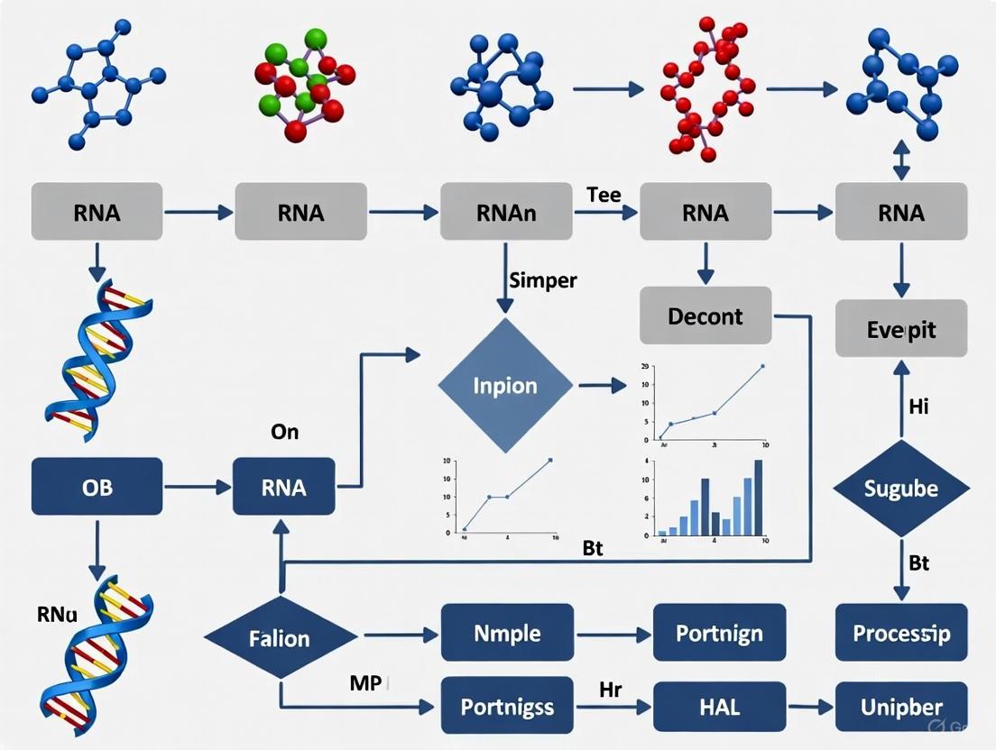
RNA sequencing (RNA-seq) is a fundamental technique in molecular biology that enables detailed analysis of the transcriptome. This technical support guide details the critical steps and considerations for the preprocessing phase of RNA-seq data analysis, which transforms raw sequencing data (FASTQ files) into a gene count matrix suitable for downstream differential expression and other bioinformatic analyses. This process is a cornerstone of reproducible research and is vital for extracting accurate biological insights from transcriptomic data [1] [2].
The following workflow provides a high-level overview of the primary steps in the RNA-seq preprocessing pipeline, from raw data to a normalized count matrix.
Troubleshooting Guides
Troubleshooting RNA Extraction and Quality
Successful RNA-seq analysis begins with high-quality RNA. The table below outlines common RNA extraction issues, their causes, and recommended solutions [3].
| Problem | Causes | Solutions |
|---|---|---|
| RNA Degradation | RNase contamination; improper storage; repeated freeze-thaw cycles. | Use RNase-free reagents and equipment; store samples at -85°C to -65°C; aliquot samples to avoid freeze-thaw cycles [3]. |
| Low Purity (Downstream Inhibition) | Protein, polysaccharide, or fat contamination; salt residue. | Reduce starting sample volume; increase volume of lysis reagent; increase number of ethanol rinses [3]. |
| Genomic DNA Contamination | High sample input; incomplete removal of DNA during extraction. | Reduce sample input volume; use reverse transcription reagents with a genomic DNA removal module [3]. |
| Low RNA Yield | Excessive sample amount; inadequate lysis reagent volume; incomplete homogenization. | Adjust sample amount to ensure effective homogenization; ensure sufficient volume of lysis reagent (e.g., TRIzol) [3]. |
Troubleshooting Computational Preprocessing
Issues can also arise during the computational steps of the pipeline. Key considerations for experimental design and tool selection are critical for ensuring data quality [1] [2].
| Problem | Causes | Solutions |
|---|---|---|
| Poor Read Alignment | Incorrect alignment tool parameters; high sequence divergence; adapter contamination. | Use splice-aware aligners (e.g., STAR); trim adapter sequences with tools like fastp or Trim Galore; consider species-specific optimization of parameters [1]. |
| Technical Variation & Batch Effects | Library preparation batch effects; differences in flow cell or sequencing lane. | Multiplex samples across lanes; use a randomized or blocked experimental design; apply batch effect correction tools (e.g., ComBat, Limma) during normalization [4] [5] [2]. |
| Inaccurate Quantification | PCR duplicates; ambiguous read mapping; not accounting for gene length or sequencing depth. | For single-cell data, use UMIs to collapse PCR duplicates; use quantification tools (e.g., Salmon, Kallisto) that are aware of transcript length and library depth [5] [6]. |
Frequently Asked Questions (FAQs)
Q1: What is the difference between FASTA and FASTQ file formats? The FASTA format contains sequence data (nucleotide or amino acid) preceded by a description line starting with a ">" symbol. The FASTQ format, used for raw sequencing data, extends this by including quality scores for each base call in the sequence, which are essential for quality control [7] [8].
Q2: Why is normalization necessary in RNA-seq, and what are the common methods? Normalization adjusts raw count data to remove technical variations (e.g., sequencing depth, gene length) that would otherwise mask true biological differences [5]. Common methods include:
- Within-sample: TPM (Transcripts Per Million) and FPKM/RPKM adjust for sequencing depth and gene length, allowing for comparisons of expression between different genes within the same sample [5].
- Between-sample: TMM (Trimmed Mean of M-values) assumes most genes are not differentially expressed and calculates scaling factors relative to a reference sample to compare expression across samples [5].
Q3: What is a "batch effect" and how can it be corrected? A batch effect is technical variation introduced when samples are processed in different groups (batches), such as on different days or by different personnel. This variation can confound biological results [4] [5]. Computational correction methods like ComBat (which uses empirical Bayes statistics) and tools in the Seurat package can be used to remove these effects after normalization, provided the batch information is known [4] [5].
Q4: How are PCR duplicates handled differently in bulk vs. single-cell RNA-seq? In bulk RNA-seq, duplicates are often removed based on their genomic start and end coordinates. In single-cell RNA-seq, Unique Molecular Identifiers (UMIs) are used. Reads with the same UMI that map to the same gene are considered technical duplicates from PCR amplification and are collapsed into a single count, while reads with different UMIs are considered to come from original mRNA molecules and are counted separately [6].
Q5: What are the key considerations for designing an RNA-seq experiment?
- Replicates: Biological replicates (samples from different individuals/conditions) are essential for capturing biological variance and should be prioritized over technical replicates [2].
- Sequencing Depth and Read Length: Sufficient depth is needed to detect expressed genes, especially those with low expression. Longer reads (e.g., paired-end) can improve alignment accuracy and the ability to detect alternative splicing events [2].
- Randomization: To avoid confounding batch effects with biological conditions, samples from all experimental groups should be randomized during library preparation and sequencing [2].
The Scientist's Toolkit: Research Reagent Solutions
The following table lists essential tools, software, and materials used in a typical RNA-seq preprocessing workflow.
| Item | Function in the Pipeline |
|---|---|
| fastp / Trim Galore | Used for quality control, adapter trimming, and filtering of low-quality reads from raw FASTQ files [1]. |
| STAR | A splice-aware aligner that accurately maps RNA-seq reads to a reference genome, accounting for intron-exon boundaries [6] [2]. |
| Salmon / Kallisto | Tools for transcript quantification. They use lightweight alignment or pseudoalignment to rapidly estimate the abundance of transcripts from RNA-seq data [6] [8]. |
| UMI-tools / zUMIs | Software packages designed to process single-cell RNA-seq data, including the demultiplexing of samples and collapsing of PCR duplicates using UMIs [6]. |
| EdgeR / DESeq2 | R packages used for downstream differential expression analysis. They require a normalized count matrix as input and employ statistical models based on the negative binomial distribution [2]. |
| Cell Ranger | A specialized pipeline (from 10x Genomics) for processing single-cell RNA-seq data generated using their platform, handling all steps from demultiplexing to count matrix generation [6]. |
Optimized Workflow and Normalization Strategies
As part of thesis research on workflow optimization, it has been demonstrated that the default parameters of analysis software are not universally optimal across all species. A comprehensive study testing 288 analysis pipelines on fungal data established that careful selection and tuning of tools at each step can provide more accurate biological insights than using default configurations [1]. The diagram below illustrates the key decision points and strategies for normalization and batch effect correction within an optimized workflow.
FAQs on Experimental Design
Q1: What is the minimum number of biological replicates required for a robust RNA-seq experiment?
Biological replicates are essential for capturing the natural variation within a population and are a prerequisite for statistical significance testing in differential expression analysis. The absolute minimum is 3 replicates per condition [9], with 4 being the optimum minimum [9]. This is because most statistical algorithms used for differential expression, such as DESeq2, require a minimum of 3 samples per group to function correctly [10]. Treating cells from a single sample as replicates in single-cell RNA-seq is a statistical mistake; biological replicates (multiple independent samples) are still necessary, and methods like "pseudobulking" should be used to account for between-sample variation [11].
Q2: How do I choose between sequencing depth and the number of replicates when resources are limited?
When facing budget constraints, the general recommendation is to prioritize the number of biological replicates over extreme sequencing depth [12]. More replicates provide a better estimate of biological variance, which increases the statistical power to detect differentially expressed genes. A well-replicated study with modest depth is more robust than an under-replicated one sequenced very deeply. If possible, a staged sequencing approach can be a compromise, where the same samples are sequenced in multiple runs and the data is combined later [12].
Q3: Should I use paired-end or single-end sequencing for my experiment?
The choice depends on your research goals. Paired-end (PE) sequencing is preferable for applications like de novo transcript discovery, isoform expression analysis, and alternative splicing studies because it provides more mapping information [13]. For standard gene expression profiling in well-annotated organisms, the cheaper single-end (SE) reads are often sufficient [13]. The NIH CCBR also notes that single-end sequencing is typically the most economical option [9].
Q4: How does my library preparation method impact the data I can generate?
The library preparation method directly determines the type of RNA species you can analyze and the applications possible [12]. The key decision is often between a 3' enrichment method and a whole transcriptome approach.
- 3' mRNA-Seq: This method is cost-effective and excellent for gene expression profiling. However, as reads are localized to the 3' end of transcripts, it is not suitable for investigating alternative splicing, differential transcript usage, or transcript isoform identification [12].
- Whole Transcriptome Sequencing: This provides full transcript coverage and is necessary for the analyses mentioned above. It requires either poly(A) enrichment (for coding mRNA) or rRNA depletion (for non-coding RNAs or degraded samples) [13] [12]. The table below summarizes these choices.
Table 1: Choosing a Library Preparation Method
| Method | Best For | Pros | Cons |
|---|---|---|---|
| 3' mRNA-Seq | Gene expression profiling, high-throughput projects [12] | Highly multiplexable, minimal computational resources needed [12] | Not suitable for splicing or isoform analysis [12] |
| Whole Transcriptome (Poly(A)) | Analyzing polyadenylated mRNA (coding) [13] [12] | Focuses on mRNA; high fraction of exonic reads [13] | Requires high-quality RNA (RIN >8); misses non-polyA RNA [13] [9] |
| Whole Transcriptome (rRNA depletion) | Non-coding RNAs, degraded samples (e.g., FFPE), prokaryotes [13] [12] | Works with degraded RNA; captures both coding and non-coding RNA [12] | More expensive; higher ribosomal RNA residue possible [13] |
Q5: How can I avoid batch effects in my RNA-seq study?
Technical variation from library preparation and sequencing lanes is a major source of batch effects [2]. To minimize this:
- Process all RNA extractions simultaneously. Extractions done at different times can introduce strong batch effects [9].
- Multiplex your samples. If possible, all samples should be indexed, pooled, and run across all sequencing lanes to confound lane effects with other variables [2] [9].
- Use a blocking design. If full multiplexing is impossible, ensure that replicates for each experimental condition are distributed across all processing batches and sequencing lanes. This allows bioinformatic tools to measure and correct for these technical effects later [2] [9].
Troubleshooting Guides
Problem: Inconsistent or statistically weak differential expression results.
- Potential Cause 1: Insufficient replicates.
- Solution: Increase the number of biological replicates. With only 2 replicates, it is impossible to reliably estimate biological variance, and statistical power is very low. Plan for at least 3-4 biological replicates per condition [9].
- Potential Cause 2: Confounding batch effects.
- Solution: Review your experimental metadata. If samples were processed in batches, use statistical models in your differential expression analysis (e.g., in DESeq2) to include "batch" as a covariate to correct for its effect [9].
- Potential Cause 3: Incorrect analysis for single-cell data.
- Solution: Do not treat individual cells as biological replicates. Use a "pseudobulk" approach, where counts are aggregated for each cell type within each biological sample, and then standard bulk RNA-seq differential expression tools are applied to these aggregated counts [11].
Problem: Low mapping rates or biased coverage.
- Potential Cause 1: Poor RNA quality.
- Potential Cause 2: Inadequate read trimming.
- Potential Cause 3: Incorrect library type for the organism.
The Scientist's Toolkit: Key Reagents and Materials
Table 2: Essential Research Reagents and Materials for RNA-seq
| Item | Function |
|---|---|
| RNA Extraction Kit | Isolates high-quality total RNA from cells or tissues. The choice of kit may vary based on sample type (e.g., bacterial vs. mammalian) and RNA species of interest (e.g., small RNAs) [12] [10]. |
| Library Preparation Kit | Converts purified RNA into a sequencing-compatible library. The specific kit determines the scope of the experiment (e.g., 3' counting, whole transcriptome, small RNA) [12] [10]. |
| Poly(dT) Magnetic Beads | Used in poly(A) selection to enrich for messenger RNA by binding to the poly-adenylated tail. This removes ribosomal RNA (rRNA) [13]. |
| Ribosomal RNA Depletion Probes | Probes that hybridize to and remove abundant rRNA, allowing for the sequencing of other RNA species. Essential for prokaryotes, non-polyA RNAs, or degraded samples [13] [12]. |
| Spike-in Control RNAs (e.g., ERCC, SIRV) | Synthetic RNA molecules added to the sample in known quantities. They are used to assess technical performance, detect amplification biases, and sometimes to aid in normalization [12]. |
| Unique Molecular Identifier (UMI) Adapters | Adapters containing random molecular barcodes that tag individual RNA molecules before amplification. This allows for the accurate counting of original transcript molecules and correction for PCR duplication bias [11]. |
Experimental Design and Analysis Workflow
The following diagram outlines the key decision points and their consequences in planning an RNA-seq study, integrating the concepts of replicates, library preparation, and sequencing strategy.
To ensure the success of your RNA-seq experiment and the optimization of your preprocessing workflow, adhere to these core principles:
- Replicate Power: Biological replicates are non-negotiable. Plan for a minimum of 3, and ideally 4 or more, independent biological replicates per condition to ensure statistically robust results [9].
- Design to Control Batch Effects: From the start, design your experiment to minimize technical confounding. Process samples randomly and use multiplexing across sequencing lanes to make batch effects measurable and correctable [2] [9].
- Align Methods with Goals: Let your biological question dictate your technical choices. If studying isoform usage, you must use a whole transcriptome, paired-end sequencing approach. For simple gene counting, 3' mRNA-Seq is sufficient and more cost-effective [13] [12].
- Validate with a Pilot Study: Before launching a large-scale project, conduct a pilot experiment with a representative subset of samples. This allows you to verify that your chosen RNA quality, library preparation, and sequencing depth parameters will deliver the data required to answer your research question [12].
FAQs and Troubleshooting Guides
This guide addresses common questions and issues researchers encounter when working with key file formats in the RNA-seq preprocessing workflow. Proper handling of these formats is crucial for generating accurate and reproducible results in transcriptome analysis.
FASTQ Format
What is the basic structure of a FASTQ file? Each sequence in a FASTQ file consists of exactly four lines [14] [15]:
- Sequence Identifier and Description: Begins with an
@character and contains information about the sequencing run and the cluster [14] [16]. - The Sequence: The actual base calls (A, C, T, G, N) [14].
- A Separator: A
+sign, which may optionally be followed by the same sequence identifier [14]. - Quality Scores: Encoded quality scores for each base in the sequence line. The length of this line must match the length of the sequence line [14] [16]. The scores are Phred-scaled and typically use ASCII characters with an offset of 33 (Sanger encoding) [15].
How can I quickly check the number of reads in a FASTQ file? You can use command-line tools:
- Using
seqkit stats: The commandseqkit stats your_file.fqprovides comprehensive statistics, including the number of sequences [14]. - Using basic Bash commands: The command
echo $(( $(wc -l < your_file.fq) / 4 ))calculates the number of records by dividing the total line count by four [16].
My FASTQ files are too large to open in a text editor. How can I view them? FASTQ files are not meant to be opened in standard text editors due to their size [15]. Use command-line tools instead:
- Use
head -n 4 your_file.fqto view the first read [14]. - Use
zcatfor compressed.gzfiles (e.g.,zcat your_file.fastq.gz | head -n 4).
How do I combine multiple FASTQ files from the same sample?
You can consolidate files using the cat command. However, for a large number of files, a more robust method is recommended [16]:
The base quality of my reads is low. What should I do? Low quality at the 3' end of reads is common. Use trimming/filtering tools like fastp or Trim Galore (which integrates Cutadapt and FastQC) to remove low-quality bases and adapter sequences before proceeding to alignment [1]. This step can significantly improve the subsequent mapping rate [1].
SAM/BAM Format
What is the difference between SAM and BAM files?
- SAM (Sequence Alignment Map) is a human-readable, tab-delimited text format [17].
- BAM is the compressed binary version of SAM. It is much smaller in size and allows for efficient indexing and random access, which is required by many downstream analysis tools [17].
What are the mandatory fields in a SAM/BAM alignment record? Each alignment line has 11 mandatory fields [18]:
Table: Mandatory Fields in a SAM/BAM File
| Col | Field | Type | Brief Description |
|---|---|---|---|
| 1 | QNAME | String | Query template name (read identifier) |
| 2 | FLAG | Integer | Bitwise flag encoding multiple properties (e.g., paired-end, strand, mapping quality) |
| 3 | RNAME | String | Reference sequence name the read aligns to |
| 4 | POS | Integer | 1-based leftmost mapping position of the first aligned base |
| 5 | MAPQ | Integer | Mapping quality, indicating the reliability of the alignment (-10log10(Pr(mapping position is wrong))) |
| 6 | CIGAR | String | String that describes the alignment (e.g., matches, deletions, insertions, splicing) |
| 7 | RNEXT | String | Reference name of the mate/next read |
| 8 | PNEXT | Integer | Position of the mate/next read |
| 9 | TLEN | Integer | Observed template length (insert size) |
| 10 | SEQ | String | The raw sequence itself |
| 11 | QUAL | String | The base quality scores, encoded in the same Phred+33 format as the FASTQ file |
How do I interpret the bitwise FLAG field?
The FLAG is an integer that is the sum of numeric codes representing different alignment attributes. For example, a FLAG value of 99 (64 + 32 + 2 + 1) for a paired-end read means: the read is paired, it is the first read in the pair, its mate is mapped, and both reads are mapped in a proper pair. Use online tools like the SAMflag tool or the samtools flag command to decode these values [18].
My downstream tool requires a sorted BAM file. How do I create one?
Use samtools sort. Sorting by coordinate is essential for many tasks, including variant calling and visualization [17].
The -@ option allows you to use multiple threads to speed up the process [17].
How can I view alignments for a specific genomic region?
You first need to index the sorted BAM file and then use samtools view [17].
What is the CIGAR string and why is it important for RNA-seq?
The CIGAR (Compact Idiosyncratic Gapped Alignment Report) string describes how a read aligns to the reference. It is crucial for RNA-seq because it can represent spliced alignments. Operations like N (skipped region from the reference) denote introns, showing where splicing has occurred. For example, a CIGAR string of 50M1000N50M means 50 bases match the reference, then 1000 bases are skipped (an intron), followed by another 50 matching bases [17].
GTF/GFF3 Format
What is the difference between GFF3 and GTF files? While both are 9-column, tab-delimited formats for genomic annotations, they have key differences in history and usage [19] [20]:
Table: Comparison of GFF3 and GTF File Formats
| Aspect | GTF (Gene Transfer Format) | GFF3 (General Feature Format version 3) |
|---|---|---|
| Origin & Focus | Evolved from GFF2; more gene-centric. | Developed by the Sequence Ontology Project; broader scope for all genomic features (genes, RNAs, regulatory regions). |
| Feature Types (3rd column) | Limited types (e.g., gene, transcript, exon, CDS, UTR) [19]. |
A wider variety of types (e.g., gene, mRNA, tRNA, ncRNA, chromosome, biological_region) [19]. |
| Attribute Column (9th column) | Uses specific, structured key-value pairs (e.g., gene_id "ENSG000001"; transcript_id "ENST000001"). |
More flexible key-value pairs. Uses a flat list of tags. Relationships are often defined with the Parent tag. |
| Hierarchy Representation | Implied hierarchy based on shared gene_id and transcript_id attributes. |
Explicit hierarchy using the ID and Parent attributes to build a tree structure. |
Should I use GTF or GFF3 for RNA-seq analysis?
For standard RNA-seq differential expression analysis, the GTF format from Ensembl is most commonly used. Its structured attribute column with consistent gene_id and transcript_id tags is directly compatible with quantification tools like featureCounts and HTSeq [20]. However, always check which format your specific analysis tool requires.
The gene IDs in my GTF/GFF3 file do not match the ones in my expression matrix. What is wrong?
This is a common issue. The problem often lies in the version numbers of the gene identifiers. For example, ENSG000001 and ENSG000001.5 are treated as different IDs. Ensure that the annotation file (GTF/GFF3) and the reference genome used for alignment are from the same source and version. Mismatches can lead to failed quantification.
How can I convert between GFF3 and GTF formats? Use dedicated bioinformatics tools like AGAT or GenomeTools to convert between formats while preserving the integrity of the annotation information [20]. For example, to convert GFF3 to GTF with AGAT:
The Scientist's Toolkit
Table: Essential Tools and File Formats for RNA-seq Preprocessing
| Item Name | Function / Role in the Workflow |
|---|---|
| FastQC | Generates a quality control report for raw or trimmed FASTQ files, highlighting potential issues [14]. |
| fastp / Trim Galore | Performs adapter trimming and quality filtering of FASTQ reads to improve downstream mapping [1]. |
| STAR / HISAT2 | Aligns (maps) sequencing reads from FASTQ files to a reference genome, producing SAM/BAM files. |
| SAMtools | A versatile toolkit for manipulating SAM/BAM files, including sorting, indexing, and filtering [17]. |
| BAM Index (.bai) | A separate index file for a sorted BAM file that enables fast random access to genomic regions [17]. |
| Ensembl GTF Annotation | Provides gene model annotations, defining the coordinates of genes, transcripts, and exons for read quantification [19] [20]. |
| seqkit | A cross-platform and efficient toolkit for FASTA/Q file manipulation [14] [16]. |
Experimental Protocols and Data
Protocol: Assessing FASTQ File Quality with FastQC and seqkit
- Obtain Basic Statistics: Run
seqkit stats *.fqto get a quick overview of read counts and average read lengths for all your files [14]. - Generate a Quality Report: Run
fastqc *.fqto start the analysis. FastQC will process each file and generate an HTML report [14]. - Interpret Key FastQC Modules:
- Per Base Sequence Quality: Check that quality scores are high (e.g., >Q28) across all bases, with a common drop at the read ends.
- Per Base Sequence Content: The four lines for A, C, G, T should be roughly parallel. Deviations can indicate adapter contamination or overrepresented sequences.
- Overrepresented Sequences: Identifies sequences (like adapters) that appear much more frequently than others.
Quantitative Data from a Typical RNA-seq Run
The table below shows example statistics generated by seqkit stats for a paired-end RNA-seq dataset, illustrating the consistency expected between read pairs (R1 and R2) [14]:
Table: Example FASTQ File Statistics for HBR and UHR Samples
| File | Format | Type | Number of Sequences | Average Length (bp) |
|---|---|---|---|---|
| HBR1R1.fq | FASTQ | DNA | 118,571 | 100 |
| HBR1R2.fq | FASTQ | DNA | 118,571 | 100 |
| HBR2R1.fq | FASTQ | DNA | 144,826 | 100 |
| HBR2R2.fq | FASTQ | DNA | 144,826 | 100 |
| UHR1R1.fq | FASTQ | DNA | 227,392 | 100 |
| UHR1R2.fq | FASTQ | DNA | 227,392 | 100 |
Workflow Visualization
The following diagram illustrates the role of each file format within a standardized RNA-seq preprocessing workflow, which is critical for optimization research [1].
Frequently Asked Questions
Q1: What is RNA-seq strandedness and why is incorrectly specifying it so detrimental? Strandedness refers to whether the RNA-seq library preparation protocol preserves the original orientation (strand) of the RNA transcript. Incorrectly specifying this parameter during analysis can lead to severe consequences, including:
- Loss of >95% of reads during mapping to a reference [21].
- Increased false positives and negatives in differential expression analysis, with one study noting over 10% false positives and over 6% false negatives [21].
- Compromised accuracy in transcript assembly and quantification, especially for genes that overlap on opposite strands [21] [13].
Q2: How can I quickly determine the strandedness of my RNA-seq data if it's not documented? If strandedness is unavailable from metadata or the sequencing facility, you can use dedicated tools.
how_are_we_stranded_here: A Python library designed to quickly infer strandedness from paired-end RNA-seq data. It works by pseudoaligning a sample of reads (default: 200,000) to a transcriptome and then usingRSeQC's infer_experiment.pyto determine the read orientation relative to transcripts. It is fast, with runs often taking less than a minute [21] [22].RSeQC's infer_experiment.py: This tool can be run directly on an aligned BAM file. It samples reads and compares their genomic coordinates and strand to a reference gene model to gauge the strand-specific protocol used [23].
Q3: Should I always discard single-end (SE) reads from a paired-end (PE) library during pre-processing? Not necessarily. Common practice involves:
- Processing PE reads where both pairs pass quality filtering as proper pairs.
- Retaining reads where only one of the pair passes filtering as a single-end read. This prevents the loss of valuable data that still indicates the presence of a transcript [24] [25]. These "orphaned" reads are typically counted as one fragment, the same as a properly aligned pair [24].
Q4: What is a Q30 quality score and why is it considered a benchmark? The Phred Quality Score (Q score) measures the probability that a base was called incorrectly by the sequencer [26] [27]. A score of Q30 means there is a 1 in 1,000 probability of an incorrect base call, which translates to a base call accuracy of 99.9% [26]. This benchmark ensures that virtually all reads are perfect, minimizing false-positive variant calls and providing a high-confidence foundation for downstream analysis [26].
Experimental Protocols for Key Determinations
Protocol 1: Quick Strandedness Determination usinghow_are_we_stranded_here
This protocol is designed for rapid, pre-alignment quality control [21].
- Installation: Install the library via pip (
pip install how_are_we_stranded_here) or conda (conda install --channel bioconda how_are_we_stranded_here). - Prerequisite: Obtain the transcriptome FASTA and GTF annotation files for your organism.
- Indexing: Create a kallisto index of the organism's transcriptome. Note: This is the most time-consuming step (e.g., ~6-7 minutes for human) but is reusable for the same species [21].
- Execution: Run the tool on your paired-end FASTQ files. By default, it samples 200,000 reads for pseudoalignment.
- Interpretation: The tool outputs a "stranded proportion."
- Proportion ~1.0: Data is stranded (all reads explained by one orientation).
- Proportion ~0.5: Data is unstranded (a near-even mix of orientations) [21].
Protocol 2: Strandedness Determination from a BAM File usingRSeQC
Use this protocol if you already have aligned BAM files [23].
- Tool Setup: Ensure RSeQC is installed, with
infer_experiment.pyaccessible. - Data Preparation: Convert your GTF annotation file to BED12 format using the
gtf2bedscript or a similar tool. - Execution: Run
infer_experiment.pyon your sorted BAM file, providing the BED12 file as the reference gene model. - Interpretation: The tool reports the fraction of reads explained by "1++,1--,2+-,2-+" (FR/Second Strand) and "1+-,1-+,2++,2--" (RF/First Strand).
- If one fraction is >0.9, your data is stranded, and you should use the corresponding layout.
- If the two fractions are close to 0.5, your data is unstranded [23].
Structured Data for Easy Comparison
Table 1: Decoding Strandedness Terminology Across Software
Software tools use different terms for the same library types. This table helps translate between them [23].
| Library Type | Infer Experiment (RSeQC) Output |
HISAT2 | featureCounts | HTSeq-Count |
|---|---|---|---|---|
| PE - SF | "1++,1--,2+-,2-+" | --rna-strandness F |
-s 1 |
--stranded=yes |
| PE - SR | "1+-,1-+,2++,2--" | --rna-strandness R |
-s 2 |
--stranded=reverse |
| SE - SF | "++,--" | --rna-strandness F |
-s 1 |
--strended=yes |
| SE - SR | "+-,-+" | --rna-strandness R |
-s 2 |
--stranded=reverse |
| Unstranded | Undecided / ~50% split | --rna-strandness unspecified |
-s 0 |
--stranded=no |
Table 2: Interpreting Sequencing Quality Scores
This table defines standard quality thresholds used in data trimming and filtering [26] [27].
| Quality Score (Q) | Probability of Incorrect Base Call | Base Call Accuracy | Common Application in RNA-seq |
|---|---|---|---|
| Q20 | 1 in 100 | 99% | A common, though lenient, threshold for trimming low-quality bases [27]. |
| Q30 | 1 in 1,000 | 99.9% | The benchmark for high-quality data; ensures virtually all reads are perfect [26]. |
The Scientist's Toolkit
Table 3: Essential Research Reagent Solutions
| Item | Function in RNA-seq Preprocessing |
|---|---|
| FastQC | Provides an initial quality report on raw sequence data in FASTQ files, assessing per-base sequence quality, GC content, adapter contamination, and more [25] [13]. |
| Trimmomatic / fastp | Performs adapter trimming and removal of low-quality bases to clean the raw reads, which is crucial for improving downstream mapping rates [1] [25] [13]. |
| RSeQC | A suite of tools for comprehensive quality control on RNA-seq data after alignment, including the vital infer_experiment.py for strandedness determination [21] [23] [13]. |
| STAR / HISAT2 | "Splice-aware" aligners that accurately map RNA-seq reads to a reference genome, accounting for reads that span exon-intron junctions [25] [13]. |
| kallisto | A pseudoaligner used for fast transcript-level quantification and a key component of the how_are_we_stranded_here workflow [21]. |
Workflow Diagrams
Strandedness Determination Workflow
RNA-seq Preprocessing Quality Control
A Step-by-Step Guide to Implementing a Robust Preprocessing Pipeline
Core Concepts: FastQC and MultiQC
What are FastQC and MultiQC, and what are their primary functions in an RNA-seq workflow?
FastQC is a quality control tool that provides a simple way to perform initial quality checks on raw sequence data from high-throughput sequencing pipelines. Its main functions are to import data from BAM, SAM, or FastQ files; provide a quick overview of potential problem areas; generate summary graphs and tables for rapid data assessment; and export results to HTML-based reports for easy sharing and documentation [28] [29].
MultiQC is an aggregation tool that searches specified directories for analysis logs and compiles them into a single interactive HTML report. It is particularly valuable in RNA-seq workflows for comparing QC metrics across all samples simultaneously, enabling researchers to quickly identify outliers and consistency issues. MultiQC can parse output from 36 different bioinformatics tools, including FastQC, STAR, Qualimap, and Salmon, providing a unified view of quality throughout the RNA-seq pipeline [30].
What is the fundamental structure of a FASTQ file, and how are quality scores encoded?
A FASTQ file contains sequence reads with quality information and follows a specific four-line structure for each record [28]:
- Line 1: Always begins with '@' followed by information about the read
- Line 2: The actual DNA sequence
- Line 3: Always begins with a '+' and sometimes contains the same information as line 1
- Line 4: Has a string of characters representing quality scores; must contain the same number of characters as line 2
Quality scores (Phred scores) are encoded as ASCII characters and represent the probability that a base was called incorrectly. The most commonly used encoding is fastqsanger (Phred-33). The quality score is calculated as Q = -10 × log10(P), where P is the probability that a base call is erroneous [28].
Table: Interpretation of Phred Quality Scores
| Phred Quality Score | Probability of Incorrect Base Call | Base Call Accuracy |
|---|---|---|
| 10 | 1 in 10 | 90% |
| 20 | 1 in 100 | 99% |
| 30 | 1 in 1000 | 99.9% |
| 40 | 1 in 10,000 | 99.99% |
Troubleshooting Common FastQC Issues
Why does my RNA-seq data "fail" Per base sequence content, and is this truly problematic?
This is a common concern. The "Per base sequence content" module often raises a failure flag for RNA-seq data due to non-randomness in the first 10-12 bases, which is actually expected behavior rather than indicating poor data quality [31].
Root Cause: During RNA-seq library preparation, 'random' hexamer priming occurs. This priming is not perfectly random, leading to an enrichment of particular bases in these initial nucleotide positions. This bias is a technical artifact of the library preparation method, not a sequencing error.
Assessment & Solution: This "failure" can generally be ignored for RNA-seq data, as it reflects expected biological protocol limitations rather than sequencing quality issues. Most alignment tools (STAR, HISAT2, Salmon) can adequately handle this bias during mapping [31].
Why do I see a drop in quality scores toward the end of reads, and when should I be concerned?
A gradual decrease in quality toward the 3' end of reads is common in Illumina sequencing and can result from two expected phenomena [31]:
- Signal Decay: Fluorescent signal intensity naturally decays with each sequencing cycle due to degrading fluorophores and a proportion of strands in the cluster not elongating.
- Phasing: As cycles progress, clusters lose synchronicity as some strands experience random failure of nucleotides to incorporate, leading to signal blurring.
Worrisome patterns that warrant contacting your sequencing facility include [31]:
- Sudden, dramatic drops in quality scores at specific positions
- Consistently low quality scores across the entire read length
- Large percentages of reads with low average quality scores
Table: Interpreting Quality Score Patterns in FastQC
| Pattern | Likely Cause | Action Required |
|---|---|---|
| Gradual decrease at 3' end | Expected signal decay/phasing | None typically needed |
| Sharp, sudden quality drop | Instrument failure | Contact sequencing facility |
| Consistently low scores across all bases | Overclustering or poor sequencing | Contact sequencing facility |
| Small bump of low-quality reads | Minor sequencing issue | Check if percentage is significant |
My MultiQC report shows conflicting pass/fail status between different quality metrics. How should I interpret this?
This situation, where samples pass one quality metric but fail another, requires careful interpretation of the underlying data rather than relying solely on the pass/fail status [32].
Example Scenario: In one case, samples showed "good" results for per sequence quality scores (all samples passed) but "failed" for sequence quality histograms showing mean quality scores for each base position. The solution was to recognize that while the overall average quality was high (>35), FastQC's failure trigger was based on lower quartile values falling below thresholds at specific base positions [32].
Interpretation Strategy:
- Focus on the actual data trends rather than binary pass/fail indicators
- Check if "failures" occur in expected areas (e.g., first few bases in RNA-seq)
- Compare metrics across all samples to identify true outliers
- Use MultiQC's interactive features to explore the underlying data behind each metric
Experimental Protocols
Protocol: Running FastQC Quality Assessment
Objective: Assess quality of raw RNA-seq FASTQ files using FastQC [28].
Materials Needed:
- Raw FASTQ files from RNA-seq experiment
- Computer cluster with SLURM scheduler or local compute environment
- FastQC software module
Methodology:
- Access Computing Environment: Start an interactive session on the cluster:
Navigate to Data Directory:
Load FastQC Module:
Run FastQC with Multi-threading (using 6 cores for 6 FASTQ files):
Organize Results:
Alternative Job Submission Script:
For larger datasets, create a job submission script (mov10_fastqc.run) with SLURM directives [28]:
Protocol: Generating MultiQC Reports for Cross-Sample Comparison
Objective: Aggregate and compare QC metrics from multiple tools and samples using MultiQC [30].
Materials Needed:
- Output from FastQC, STAR, Qualimap, and/or Salmon
- MultiQC software module
Methodology:
- Create Output Directory:
Load MultiQC Module:
Run MultiQC (example with multiple tool outputs):
Transfer and View Report: Use FileZilla or SCP to transfer the HTML report to your local machine for viewing in a web browser.
Protocol: Comprehensive RNA-seq QC Assessment
Objective: Perform complete quality assessment from raw reads to alignment statistics [30] [25].
Key Metrics to Track:
- Number of raw reads
- Percentage of reads aligned to genome
- Percentage of reads associated with genes
- Sequence duplication levels
- 5'-3' bias
- GC content distribution
Assessment Guidelines:
- Alignment Rates: A good quality sample should have at least 75% of reads uniquely mapped. Values below 60% warrant troubleshooting [30].
- Sequence Duplication: High duplication percentages may indicate low library complexity or over-amplification [30].
- 5'-3' Bias: Investigate biases approaching 0.5 or 2, which could indicate RNA degradation or sample preparation issues [30].
- Exonic vs. Intergenic Reads: Expect >60% exonic reads for well-annotated organisms. High intergenic reads (>30%) may indicate DNA contamination [30].
Workflow Visualization
Table: Essential Software Tools for RNA-seq Quality Control
| Tool Name | Primary Function | Key Application in RNA-seq QC |
|---|---|---|
| FastQC | Raw read quality assessment | Provides initial quality metrics on raw FASTQ files, identifying adapter contamination, quality score distribution, and sequence biases [29] [25] |
| MultiQC | QC metric aggregation | Compiles results from multiple tools and samples into a single interactive report, enabling cross-sample comparison and outlier detection [30] |
| Trimmomatic | Read trimming | Removes adapter sequences and low-quality bases from reads, improving downstream alignment rates [25] |
| Trim Galore | Wrapper for trimming | Integrates Cutadapt and FastQC to perform adapter and quality trimming with automatic quality reporting [1] |
| fastp | Rapid preprocessing | Performs adapter trimming, quality filtering, and polyG tail trimming with integrated QC reporting [1] |
| STAR | Splice-aware alignment | Aligns RNA-seq reads to reference genome, providing mapping statistics and splice junction information [30] [25] |
| Salmon | Transcript quantification | Provides fast transcript-level quantification and mapping rate statistics without full alignment [30] |
| Qualimap | Alignment QC | Evaluates alignment characteristics including coverage bias, RNA-seq specificity, and 5'-3' bias [30] |
Table: Critical QC Metrics and Interpretation Guidelines
| QC Metric | Optimal Range | Potential Issue | Recommended Action |
|---|---|---|---|
| % Uniquely Mapped Reads | >75% | <60% indicates potential alignment issues | Check RNA integrity, reference genome compatibility, or alignment parameters [30] |
| % Duplicate Reads | Variable, <50% typical | High duplication suggests low complexity | Consider library preparation optimization if consistently high [30] |
| 5'-3' Bias | ~1.0 (0.8-1.2) | Values <0.5 or >2 indicate bias | May indicate RNA degradation; check RIN scores if available [30] |
| % Exonic Reads | >60% for human/mouse | <50% may indicate DNA contamination | Verify ribosomal RNA depletion efficiency [30] |
| % GC Content | Species-specific | Deviations from expected distribution | May indicate contamination or technical artifacts [31] |
| Average Quality Score | >Q30 across most bases | Scores | Consider quality trimming or contact sequencing facility [28] [25] |
Within the framework of RNA-seq preprocessing workflow optimization research, the initial steps of adapter trimming and quality filtering are paramount. These steps directly influence the quality of all subsequent analyses, including alignment accuracy, quantification reliability, and the ultimate biological interpretations derived from differential expression and alternative splicing studies [1]. Current research demonstrates that the default parameters of analysis software are often applied uniformly across data from different species without optimization. However, the performance and accuracy of these tools can vary significantly when processing data from diverse organisms, including humans, animals, plants, and fungi [1]. For laboratory researchers, navigating the complex landscape of analytical tools to construct a bespoke and efficient workflow presents a substantial challenge. This guide addresses this gap by providing a detailed, evidence-based troubleshooting resource for three predominant trimming tools—Trimmomatic, fastp, and Cutadapt—to empower researchers in building robust, optimized RNA-seq preprocessing pipelines.
Tool Comparison and Selection Guide
Selecting an appropriate trimming tool is the first critical decision in the preprocessing workflow. The choice often balances factors such as operational simplicity, processing speed, and the richness of features. The following table summarizes the key characteristics, strengths, and limitations of Trimmomatic, fastp, and Cutadapt to guide this selection.
Table 1: Comparison of Adapter Trimming and Quality Filtering Tools
| Tool | Primary Strength | Best For | Common Challenges | Citation |
|---|---|---|---|---|
| Trimmomatic | High sensitivity for adapter detection in paired-end data (palindrome mode) | Users requiring robust, proven methods for complex adapter contamination | Complex parameter setup; confusing adapter file specifications | [33] [34] [35] |
| fastp | Integrated quality control and reporting; rapid processing speed | Researchers seeking an all-in-one solution for fast preprocessing and QC | May provide different results compared to other tools on the same data | [1] [33] |
| Cutadapt | Flexible and precise handling of diverse adapter types and configurations | Applications requiring custom or non-standard adapter layouts | Requires clear understanding of 5' vs. 3' adapter definitions | [36] |
The decision process can be visualized as a workflow to help researchers select the most suitable tool based on their primary requirements.
Troubleshooting Common Adapter Trimming Issues
Trimmomatic: No Adapters Trimmed Despite Known Contamination
Problem Description: A user runs Trimmomatic with a known correct adapter sequence but the tool reports that zero reads were trimmed, even when visual inspection (e.g., via grep) confirms adapter presence in the raw FASTQ files [33].
Diagnosis and Solution: This common issue typically stems from two main sources: incorrect adapter sequence specification or misunderstanding Trimmomatic's operational modes.
- Incorrect Adapter Sequence: The sequences provided to Trimmomatic must be the reverse complement of the adapter sequences observable in the raw FASTQ files. The palindromic mode, in particular, requires this. If your adapter sequence is
AGATCGGAAGAGC, you might need to supply its reverse complement to Trimmomatic [33]. - Operational Mode Confusion: Trimmomatic has two distinct modes for adapter clipping: "simple mode" and "palindrome mode." The palindromic mode is automatically triggered based on the presence of a
/in the adapter name in the provided FASTA file (e.g.,>Prefix/1). This mode is highly sensitive for paired-end data but requires specific sequence formatting. For a fair comparison with other tools that use the "old fashioned" way of cutting, it is often recommended to avoid the palindromic mode and use the standard simple mode with the common core adapter sequence (e.g.,AGATCGGAAGAGC) [33].
Experimental Protocol for Validation: To systematically diagnose and resolve this issue, follow this protocol:
- Verify Adapter Presence: Use
grep -B1 -A2 "AGATCGGAAGAGC" your_raw_file.fastq | head -20to visually confirm adapter contamination. - Check Adapter File: Ensure your adapter FASTA file contains the correct sequences. For standard Illumina adapters, using just the common core sequence
AGATCGGAAGAGCis often sufficient and more reliable [33]. - Run a Controlled Test: Execute Trimmomatic with a minimal parameter set, ensuring you are not using the palindromic mode inadvertently. A typical command for single-end data might be:
- Compare with Alternate Tool: Run the same dataset through
fastporbbdukwith the same core adapter sequence to verify if the issue is tool-specific [33].
Inconsistent Trimming Results Across Different Tools
Problem Description: When analyzing the same dataset with Trimmomatic, fastp, and Cutadapt, the percentage of trimmed reads and bases differs drastically, leading to confusion about which result to trust [33].
Diagnosis and Solution: The discrepancies arise from several factors inherent to how these tools are designed and configured.
- Different Default Behaviors: Each tool has a unique set of default parameters and underlying algorithms for adapter detection and quality trimming. For instance, some tools may be more aggressive in quality-based trimming by default.
- Adapter Sequence and
k-merMatching: Thek-mersize used for matching (kinbbdukor similar parameters in other tools) significantly impacts sensitivity. A longerkrequires a more exact match, potentially reducing false positives but also missing partial adapter sequences [33]. - Under-the-Hood Filtering: Tools may apply additional, non-obvious filtering steps (e.g.,
tboandtpeinbbdukfor trimming one-base overlaps in paired-end data) that are not immediately apparent to the user [33].
Experimental Protocol for Harmonization: To perform a fair and consistent comparison between tools:
- Standardize the Adapter: Use the exact same core adapter sequence for all tools (e.g.,
AGATCGGAAGAGC). Do not rely on auto-detection for benchmarking [33]. - Document All Parameters: Explicitly set and document all key parameters related to stringency, such as error rates and minimum match lengths, aiming for equivalent values across tools where possible.
- Benchmark with a Subset: Use a subset of your data (e.g., 1 million reads) for rapid iteration and comparison.
- Evaluate Downstream Impact: The true test of a trimming tool's efficacy is its effect on downstream analysis. Compare the alignment rate, the percentage of uniquely mapped reads, and the number of detected genes in the subsequent RNA-seq workflow after using each tool's output [1].
fastp: Unbalanced Base Distribution After Trimming
Problem Description: After processing with fastp, while overall base quality (Q20/Q30) is improved, an unbalanced base distribution is observed in the tail of reads, potentially indicating over-trimming or a processing artifact [1].
Diagnosis and Solution: This issue, noted in benchmarking studies, suggests that while fastp effectively enhances data quality, it may introduce sequence biases in certain scenarios [1]. This can be particularly critical for applications like single-cell RNA-seq or when analyzing transcriptome ends.
- Parameter Tuning: Investigate and adjust parameters related to quality filtering and read cutting, such as
--cut_front,--cut_tail,--cut_window_size, and--cut_mean_quality. - Leverage Reporting: Use the comprehensive JSON report generated by fastp to identify the specific stage where the distribution becomes unbalanced.
- Tool Supplementation: If the issue persists, consider using fastp primarily for its speed and adapter trimming, followed by a more conservative quality trimming with another tool, or switch to an alternative like Trimmomatic's
MAXINFOtarget=0.5, which adaptively trims reads based on a balance between read length and accuracy [1] [35].
Frequently Asked Questions (FAQs)
Q1: What is the single most important parameter to get right in adapter trimming?
A1: The correct adapter sequence itself is paramount. Using the wrong sequence will lead to a failure to remove contaminants, regardless of other parameter tuning. Always confirm the adapter type used in your library preparation kit with your sequencing facility. For standard Illumina multiplexed adapters, the core sequence AGATCGGAAGAGC is a common starting point [33].
Q2: Should I trim for quality even if my data looks good and the aligner handles it? A2: Yes, it is generally considered best practice. While modern aligners are robust, proactive quality trimming improves alignment rates and reduces mis-mappings. Evidence suggests that tailored parameter configurations, as opposed to default settings, can provide more accurate biological insights [1]. Trimming low-quality bases gives a clearer picture of the actual high-quality sequence data available for downstream analysis [34].
Q3: How do I handle 5' adapters versus 3' adapters in Cutadapt?
A3: In Cutadapt, the option used defines the adapter type. Use -a for a regular 3' adapter (the adapter follows the sequence of interest) and -g for a regular 5' adapter (the adapter precedes the sequence of interest). Furthermore, you can "anchor" adapters to the starts or ends of reads for more precise matching: use -g ^ADAPTER for an anchored 5' adapter (must be at the very start of the read) and -a ADAPTER$ for an anchored 3' adapter (must be at the very end of the read) [36].
Q4: What is the recommended quality threshold for leading/trailing trimming? A4: A value of 3 is often used to remove the special Illumina 'low quality segment' (marked with a quality score of 2). For more aggressive quality-based trimming, a threshold in the range of 10-15 is common, with 15 being more conservative [35]. The choice can be informed by the quality score distribution in your FastQC report.
Table 2: Key Research Reagent Solutions for RNA-seq Preprocessing
| Item | Function/Description | Example/Note |
|---|---|---|
| Reference Materials | Provides "ground truth" for benchmarking and validating workflow performance. | Quartet and MAQC reference RNA samples with known differential expression profiles [37]. |
| Spike-in Control RNAs | Allows for monitoring of technical performance and normalization. | External RNA Control Consortium (ERCC) synthetic RNAs spiked into samples [37]. |
| Adapter Sequence Files | FASTA files containing standard Illumina adapter and primer sequences for accurate trimming. | Files like TruSeq3-SE.fa or TruSeq3-PE.fa provided with Trimmomatic [34]. |
| Quality Control Software | Assesses the quality of raw and processed sequencing data. | FastQC is the standard tool; fastp provides integrated QC [1] [34]. |
Optimizing the adapter trimming and quality filtering stage is a non-trivial yet crucial component of RNA-seq preprocessing workflow optimization. As large-scale benchmarking studies have revealed, the choice of tools and their parameters introduces a significant source of variation in final results, especially when aiming to detect subtle differential expression with clinical relevance [37]. The following integrated workflow summarizes the key steps for reliable preprocessing, from raw data to trimmed output.
The evidence is clear: a one-size-fits-all approach to RNA-seq preprocessing is suboptimal. Researchers are encouraged to benchmark their chosen tools on a subset of their data, leveraging reference materials where possible, to establish a tailored and validated preprocessing workflow that ensures the highest data quality for their specific biological questions and study systems [1] [37].
A technical support guide for researchers optimizing RNA-seq preprocessing workflows.
Accurate alignment of transcribed RNA to a reference genome is a critical step in RNA sequencing analysis, enabling the connection of genomic information with phenotypic and physiological data [38]. The choice of alignment tool directly impacts the quality of all downstream analyses, including differential gene expression and transcript isoform discovery. This guide provides a structured comparison of mainstream alignment strategies—the full-aligners HISAT2 and STAR, and the pseudoaligner Salmon—to help you select and troubleshoot the optimal tool for your specific research context within a drug development or scientific research environment.
Tool Selection Guide
1. Which tool should I choose for standard gene expression quantification in a model organism with a good reference genome?
For most standard gene expression analyses, all three tools are excellent choices, as they produce highly correlated raw count distributions and significantly overlapping differential expression results [38]. The decision often comes down to your specific computational constraints and research goals.
- Choose STAR when you prioritize high sensitivity for detecting novel splice junctions and have access to substantial computational resources (e.g., a server with >30 GB RAM for the human genome).
- Choose HISAT2 if you are working with limited memory (RAM) or need a faster runtime. It is a robust and efficient general-purpose aligner [39] [25].
- Choose Salmon when your primary goal is fast and accurate gene/transcript quantification and you are willing to forgo the generation of a genomic BAM file, which is useful for visualization but computationally expensive to create.
2. How do I approach alignment if my primary interest is in differential expression analysis for drug treatment studies?
If your goal is Differential Gene Expression (DGE) analysis, you can confidently use any of these tools with a standard downstream analysis package like DESeq2. A comparative study showed that while the raw counts from different mappers are highly correlated, the choice of the differential expression software can have a more dramatic impact on the final results than the choice of aligner itself [38]. Therefore, ensure consistency in your DGE methodology across comparisons.
3. What are the key computational considerations when choosing an aligner?
The computational profiles of these tools differ significantly, which is a crucial factor in project planning, especially when processing large datasets.
Table 1: Computational Resource Comparison of RNA-seq Aligners
| Aligner | Typical Memory Usage | Speed | Primary Index Type | Key Consideration |
|---|---|---|---|---|
| STAR | High (e.g., ~38 GB for human GRCh37) [40] | Fast, but resource-intensive [41] | Suffix Array [39] | Requires high-throughput disks for optimal scaling with multiple threads [41]. |
| HISAT2 | Lower than STAR [40] | Very fast (~3x faster than other aligners in one comparison) [39] | Graph FM-index [38] | Ideal for environments with memory limitations. |
| Salmon | Low (in quasi-mapping mode) | Very fast ("lightweight") [42] | Duplex-linked de Bruijn graph [38] | Bypasses traditional alignment, leading to significant speed and resource gains. |
4. My aligner reports many multimapped reads. Is this a problem, and how should it be handled?
Multimapped reads, which align to multiple locations in the genome due to repetitive sequences or paralogs, are a common challenge. Most aligners, including BWA and STAR, will report a quantitative measure of these multireads [39]. Tools like Salmon and kallisto have built-in statistical models to probabilistically assign these reads, which is a key advantage of their quantification-focused approach [38]. For alignment-based tools, it is standard practice to either discard multireads or use tools that can account for them in a probabilistic manner during the quantification step.
Troubleshooting FAQs
1. I am seeing a high rate of spurious spliced alignments in repetitive regions. How can I resolve this?
Widely used splice-aware aligners like STAR and HISAT2 can sometimes introduce erroneous spliced alignments between repeated sequences (e.g., Alu elements in humans) [43]. This can lead to the inclusion of falsely spliced transcripts, or "phantom" introns, in your analysis.
- Solution: Use a tool like EASTR (Emending Alignments of Spliced Transcript Reads) to post-process your alignment files. EASTR detects and removes these falsely spliced alignments by examining the sequence similarity between the flanking regions of an intron and their frequency in the genome [43]. Applying EASTR before transcript assembly has been shown to substantially reduce false positive introns, exons, and transcripts in diverse species, including human, maize, and Arabidopsis thaliana [43].
2. A large percentage of my reads are not aligning. What are the potential causes and fixes?
A high rate of unaligned reads can stem from both biological and technical issues [39].
- Potential Causes:
- Reference Mismatch: Your sample may have significant genetic polymorphisms relative to the reference genome, or the reference may be incomplete.
- Adapter Contamination: Sequencing adapters were not adequately trimmed from your raw reads.
- Low-Quality Reads: The presence of many low-quality bases prevents confident alignment.
- High RNA Complexity: Libraries prepared with rRNA-depletion (ribo-minus) methods have been observed to have a higher proportion of spurious alignments and may present more mapping challenges compared to poly(A) selected libraries [43].
- Troubleshooting Steps:
- Re-inspect Raw Reads: Use FastQC and MultiQC on your raw and trimmed FASTQ files to check for adapter content, overall quality, and GC content [25].
- Verify Trimming: Ensure your pre-processing step (using tools like Trimmomatic or Trim Galore!) successfully removed adapters and low-quality bases [25] [44].
- Check Reference Compatibility: Confirm that you are using the correct version of the reference genome and that your annotation file (GTF/GFF) matches the genome version.
3. How can I determine the strandedness of my RNA-seq library, and why is it important?
Stranded information is crucial when analyzing genomic regions with overlapping genes on opposite DNA strands. Incorrectly specifying strandedness can lead to misassignment of reads and inaccurate quantification.
- Solution: Most modern pipelines can automatically infer strandedness. For example, the nf-core/RNA-seq pipeline will sub-sample reads and use Salmon Quant to infer the strandedness, classifying the library as forward-stranded, reverse-stranded, or unstranded based on configurable thresholds [40]. The results are then displayed in the MultiQC report for verification [40]. You can also check your library preparation kit's manual, as the method (e.g., the standard dUTP method) determines the expected strand orientation.
Experimental Protocols & Workflows
Standard Operating Procedure (SOP): RNA-seq Alignment and Quantification
The following workflow outlines the key steps for RNA-seq data processing, from raw reads to gene counts [25] [42].
Phase 1: Pre-processing of Raw Reads
- Step 1.1: Quality Check. Use FastQC on raw FASTQ files to assess read quality, GC content, and adapter contamination. Collate reports across all samples with MultiQC [25].
- Step 1.2: Adapter and Quality Trimming. Use a tool like Trimmomatic or Trim Galore! to perform three key clean-up steps simultaneously [25]:
- Remove adapter sequences.
- Trim low-quality bases from the ends of reads (e.g., Phred score < 25).
- Discard reads that become very short (e.g., < 20 bases) after trimming.
- Step 1.3: Quality Re-check. Run FastQC again on the trimmed FASTQ files to confirm improvements in data quality [25].
Phase 2: Alignment and Quantification
This phase can follow one of two primary paths, as shown in the workflow diagram.
Protocol 1: Traditional Alignment-based Approach
- Alignment: Use a splice-aware aligner like STAR or HISAT2 to map reads to the reference genome. The aligner must be provided with:
- The reference genome (FASTA) and its pre-built index.
- Gene annotation file (GTF/GFF) that matches the genome version.
- Information on whether the data is single-end or paired-end and the library's strandedness [25].
- Quantification: Use a tool like featureCounts or HTSeq to generate a count matrix based on the genomic alignments (BAM files), assigning reads to genes.
- Alignment: Use a splice-aware aligner like STAR or HISAT2 to map reads to the reference genome. The aligner must be provided with:
Protocol 2: Lightweight Alignment/Pseudoalignment Approach
- Pseudoalignment and Quantification: Use Salmon (in quasi-mapping mode) or Kallisto. These tools require a reference transcriptome (FASTA) and bypass the generation of a full genomic BAM file, directly producing a count matrix of transcript abundances [42]. This method is typically much faster and less resource-intensive [42].
Phase 3: Downstream Analysis
- The final count matrix from either protocol is used for Differential Expression Analysis with tools like DESeq2 or edgeR [42].
Validation and Benchmarking Protocol
To validate your RNA-seq pipeline and results, consider this benchmarking approach:
- Housekeeping Gene Set: Identify a set of constitutively expressed genes in your dataset. Their expression should remain stable across conditions, providing a benchmark for precision [44].
- qRT-PCR Validation: Select a subset of genes (e.g., 30-32) representing high, low, and medium expression levels for validation using quantitative RT-PCR. Use a robust normalization method (e.g., global median normalization or the most stable gene) for the qRT-PCR data [44].
- Performance Metrics: Compare the RNA-seq results against the qRT-PCR gold standard to measure the accuracy and precision of the different alignment and quantification pipelines [44].
The Scientist's Toolkit
Table 2: Essential Research Reagents and Computational Tools
| Item Name | Category | Function / Application |
|---|---|---|
| STAR | Software | Spliced Transcripts Alignment to a Reference; aligns RNA-seq reads using a suffix array index [39] [25]. |
| HISAT2 | Software | Hierarchical Indexing for Spliced Alignment of Transcripts 2; uses a graph FM-index for memory-efficient alignment [38] [25]. |
| Salmon | Software | Provides fast, bias-aware quantification of transcript expression using quasi-mapping or pseudoalignment [38] [42]. |
| DESeq2 | Software | Performs differential gene expression analysis from count data using a negative binomial model [38] [42]. |
| Trimmomatic | Software | A flexible tool for the adapter removal and quality trimming of FASTQ files [25] [44]. |
| FastQC | Software | Provides quality control reports for raw sequencing data, highlighting potential issues [25]. |
| EASTR | Software | Post-alignment tool that detects and removes falsely spliced alignments in repetitive regions [43]. |
| Reference Genome (FASTA) | Data | The genomic sequence of the organism used as the alignment scaffold [25]. |
| Gene Annotation (GTF/GFF) | Data | File specifying the locations and structures of genes and transcripts on the reference genome [25]. |
| SRA Toolkit | Software | Collection of tools to access and convert data from the NCBI Sequence Read Archive (SRA) [41]. |
Frequently Asked Questions (FAQs)
Q1: A very high percentage of my reads are being reported as __no_feature by HTSeq-count. What are the primary causes?
- Incorrect Strandedness Setting: This is a very common cause. The default setting in HTSeq-count is
--stranded=yes. If your RNA-Seq library was prepared with a non-strand-specific protocol, this will cause approximately half of your reads to be lost as they will not be assigned to features on the correct strand. Always confirm your library type and set the--strandedoption accordingly (yes,no, orreverse) [45] [46]. - Mismatched Chromosome Names: The chromosome names (seqnames) in your BAM file and your GTF/GFF file must match exactly. A common discrepancy is "chr1" in the BAM file versus "1" in the GTF file, or vice versa. Visually inspect the headers of both files to ensure consistency [47] [48] [49].
- Incorrect Feature Type or Attribute: By default, HTSeq-count uses
exonas the feature--typeandgene_idas the--idattr. If your annotation file uses different values (e.g.,CDSfor type orIDfor the attribute), you must specify these parameters in the command [45] [46]. - Poor Read Alignment or Library Quality: If reads do not align correctly to genomic regions containing features, they cannot be counted. Examine your BAM files in a genome browser alongside the annotation file to verify that reads align to exonic regions. Also, check for issues like high levels of sequence duplication or overrepresented sequences from poor library construction [49].
Q2: What is the difference between HTSeq-count's union, intersection-strict, and intersection-nonempty modes?
These modes determine how a read is assigned when it overlaps multiple genomic features. The following table summarizes the three overlap resolution modes [45]:
Table: HTSeq-count Overlap Resolution Modes
| Mode | Description | Use Case |
|---|---|---|
union |
A read is counted for a feature if it overlaps the feature and any of its overlapping features do not form an set with more than one feature. This is the default and recommended for most analyses. | Standard RNA-seq analysis. Provides a balanced approach. |
intersection-strict |
A read is only counted for a feature if every single base of the read overlaps the feature. | Very conservative counting; may underestimate counts. |
intersection-nonempty |
A read is counted for a feature if at least one base of the read overlaps the feature and the read does not also overlap any other feature. | Less conservative than intersection-strict. |
Q3: My quantification tool (HTSeq-count or featureCounts) fails to run or produces zero counts, even though my BAM file has alignments. What should I check?
- File Format Validity: Ensure your BAM file is not corrupted or truncated. Use tools like
samtools quickcheckto validate the BAM file. If using a SAM file as input for HTSeq-count, confirm it has a proper header [50] [51]. - Reference Mismatch: The most severe cause is a complete mismatch between the reference genome used for alignment and the annotation file used for counting. For example, attempting to count reads aligned to a transcriptome (e.g., with XM/XP accessions) using a genome-based GTF file will fail because the coordinates are incompatible. Always use an annotation file that corresponds to the exact same reference build your reads were aligned to [47] [52].
- GTF/GFF Formatting: Check that your annotation file is properly formatted. Some tools are sensitive to header lines or specific fields. Ensure the file is not malformed [49].
Troubleshooting Guides
Diagnosis Workflow
The following diagram outlines a logical workflow for diagnosing common issues in read counting.
Guide: Resolving Strandedness Issues
Incorrect strandedness settings are a prevalent source of low count yields. This protocol provides a method to empirically determine the correct setting.
Experimental Protocol: Determining RNA-seq Library Strandedness
- Select a Subset: Isolate a subset of your BAM file (e.g., 100,000 properly aligned read pairs) using
samtools view. - Run Inferring Experiment: Use the
infer_experiment.pyscript from the RSeQC package [49].-r genes.bed: A BED file of gene coordinates.-i sample_subset.bam: Your subset BAM file.
- Interpret Output: The script will output a fraction, for example:
Fraction of reads failed to determine: 0.05Fraction of reads explained by "1++,1--,2+-,2-+": 0.90Fraction of reads explained by "1+-,1-+,2++,2--": 0.05This result indicates that 90% of reads are in the forward strand orientation, meaning the data is strand-specific. You would then use--stranded=yesin HTSeq-count. If the two fractions are roughly equal (~0.5 each), your data is unstranded, and you should use--stranded=no.
Parameter Optimization Tables
Table: Key HTSeq-count Parameters for Optimization [45]
| Parameter | Default Value | Description & Optimization Guidance |
|---|---|---|
--stranded |
yes |
Critical to check. Set to no for non-strand-specific libraries. reverse for certain stranded protocols [46]. |
--mode |
union |
Determines how reads overlapping multiple features are handled. union is recommended for most use cases [45] [46]. |
--type |
exon |
The feature type from the GTF/GFF file to count against. Must match the annotation (e.g., could be "CDS", "mRNA") [45] [46]. |
--idattr |
gene_id |
The GTF attribute used to group features into counting units. Must match the annotation (e.g., gene_id, ID, transcript_id) [45] [52]. |
--a |
10 |
Minimum alignment quality score. Reads with lower scores are skipped. Adjust if many uniquely mapped reads have low scores. |
Table: Interpretation of HTSeq-count's Special Counters [45]
| Special Counter | Description | Troubleshooting Implication |
|---|---|---|
__no_feature |
Read does not overlap any feature. | High percentage: Check strandedness, chromosome names, annotation file, or alignment quality. |
__ambiguous |
Read overlaps multiple features. | High percentage: Expected in genes with overlapping exons/UTRs. Consider a different --mode. |
__alignment_not_unique |
Read multi-mapped to the genome. | High percentage: Expected in repetitive regions. Filter your BAM for uniquely mapped reads first. |
__too_low_aQual |
Read was skipped due to low mapping quality. | Check the distribution of MAPQ scores in your BAM file. |
The Scientist's Toolkit
Table: Essential Research Reagents and Tools for Post-Alignment Quantification
| Item | Function / Explanation |
|---|---|
| SAM/BAM File | The aligned sequencing reads, the primary input for quantification. Must be sorted (by name or position) as required by the tool [45]. |
| Annotation File (GTF/GFF3) | Provides the genomic coordinates of features (e.g., genes, exons). Must be from the same genome build and have consistent chromosome naming as the BAM file [48] [49]. |
| HTSeq-count | A Python-based script to assign reads to genomic features and generate a count matrix. Highly configurable for different annotation styles [45]. |
| featureCounts | A popular alternative from the Subread package, known for fast performance and efficient handling of multi-mapping reads [46] [49]. |
| samtools | A toolkit for manipulating SAM/BAM files. Used for sorting, indexing, subsetting, and validating alignment files before quantification [45] [51]. |
| RSeQC | A Python package for RNA-seq quality control. Its infer_experiment.py script is crucial for determining library strandedness [49]. |
| Genome Browser (IGV/UCSC) | Allows visual inspection of read alignments against the reference genome and annotation tracks, which is vital for verifying assignments and troubleshooting [46] [49]. |
In RNA sequencing (RNA-seq) analysis, normalization is not merely a optional step but a fundamental prerequisite for ensuring data integrity and biological validity. It adjusts raw transcriptomic data to account for various technical factors that may mask actual biological effects and lead to incorrect conclusions [5]. The process corrects for technical variability including sequencing depth, gene length, and sample-to-sample variability [5]. This technical guide explores four prominent normalization methods—CPM, RPKM/FPKM, TPM, and TMM—with particular emphasis on their applicability for cross-sample comparison, a critical consideration in robust experimental design.
Understanding the Normalization Landscape
Why Normalization is Essential
RNA-seq generates raw count data that is influenced by multiple technical factors rather than just biological differences. Sequencing depth varies between samples, meaning a sample with more total reads will naturally have higher counts for most genes [5]. Gene length also affects quantification, as longer transcripts generate more fragments than shorter ones at the same expression level [5]. Normalization methods exist to minimize these technical variables, ensuring reliable transcriptomic data comparison [5].
The Three Stages of RNA-seq Normalization
RNA-seq normalization occurs at three distinct levels, each serving different analytical purposes:
- Within-sample normalization: Enables comparison of gene expression within an individual sample by adjusting for transcript length and sequencing depth [5].
- Within-dataset normalization (between samples): Facilitates comparison across different samples within the same experiment by accounting for technical variations like sequencing depth [5].
- Across-datasets normalization: Corrects for batch effects when integrating data from multiple independent studies sequenced at different times, with varying methods, or across multiple facilities [5].
Normalization Methods Deep Dive
CPM (Counts Per Million)
Calculation Method: CPM is calculated by dividing the raw read counts by the total number of reads in the sample (per million) [5].
Formula: CPM = (Number of reads mapped to a gene / Total mapped reads in sample) × 1,000,000 [5]
Best Use Cases:
- Simple normalization for sequencing depth only
- Preliminary data exploration
- Within-sample comparisons when used with other methods
Limitations:
- Does not normalize for gene length [5]
- Not suitable for direct between-sample comparisons of expression levels [5]
RPKM and FPKM
Calculation Method: RPKM (Reads Per Kilobase Million) for single-end data and FPKM (Fragments Per Kilobase Million) for paired-end data normalize for both sequencing depth and gene length [5] [53].
Formula: RPKM/FPKM = (Number of reads/fragments mapped to a gene × 10^9) / (Total mapped reads × Gene length in base pairs) [5]
Key Difference: FPKM accounts for the fact that two reads can correspond to a single fragment in paired-end sequencing, avoiding double-counting [53].
Best Use Cases:
- Comparing expression of different genes within the same sample [5]
- Historical data comparison (being superseded by TPM)
Limitations:
- The sum of normalized values differs between samples [53]
- Expression of a gene in one sample may appear different from another sample even at identical true expression levels [5]
TPM (Transcripts Per Million)
Calculation Method: TPM follows a different order of operations than RPKM/FPKM, normalizing for gene length first, then sequencing depth [5] [53].
Formula:
- Calculate reads per kilobase (RPK): RPK = Read counts / (Gene length in base pairs / 1,000)
- Calculate per-million scaling factor: Scaling factor = Total RPK in sample / 1,000,000
- TPM = RPK / Scaling factor [53]
Best Use Cases:
- Preferred method for within-sample comparisons [5]
- Studies requiring proportional analysis of transcript abundance
Limitations:
- Still requires between-sample normalization methods for reliable cross-sample comparisons [5]
TMM (Trimmed Mean of M-values)
Calculation Method: TMM operates under the assumption that most genes are not differentially expressed between samples [5]. It calculates scaling factors relative to a reference sample:
- One sample is designated as the reference
- Fold changes and absolute expression levels are calculated relative to the reference
- Genes are trimmed to remove differentially expressed genes
- The trimmed mean of fold changes is calculated for each sample
- Read counts are scaled by this trimmed mean [5]
Best Use Cases:
- Between-sample normalization [5]
- Differential expression analysis
- Studies with assumption that most genes are not DE
Limitations:
- Performance affected when many genes are uniquely or highly expressed in one condition [5]
Comparative Analysis of Normalization Methods
Table 1: Comprehensive Comparison of RNA-seq Normalization Methods
| Method | Normalizes For | Primary Use Case | Cross-Sample Comparison | Key Advantage | Key Limitation |
|---|---|---|---|---|---|
| CPM | Sequencing depth only | Within-sample (with other methods) | Not suitable alone [5] | Simple calculation | Does not account for gene length [5] |
| RPKM/FPKM | Sequencing depth & gene length | Within-sample gene comparison [5] | Not recommended | Gene length adjustment | Sum of normalized values varies between samples [53] |
| TPM | Sequencing depth & gene length | Within-sample comparison [5] | Better than RPKM/FPKM | Constant sum across samples [53] | Still needs between-sample methods [5] |
| TMM | Sequencing depth & composition | Between-sample normalization [5] | Excellent | Robust to differentially expressed genes [5] | Assumes most genes not DE |
Table 2: Method Suitability for Different Research Goals
| Research Goal | Recommended Method | Considerations |
|---|---|---|
| Gene expression within a sample | TPM or FPKM/RPKM [5] | TPM preferred for constant sum across samples [53] |
| Differential expression between samples | TMM or other between-sample methods [5] | TMM assumes most genes not differentially expressed [5] |
| Proportional transcript abundance | TPM [53] | TPM sum is constant, enabling proportion comparison |
| Integrating multiple datasets | Between-sample normalization + batch correction [5] | Combat or Limma recommended for batch effects [5] |
Practical Implementation and Workflow
Decision Framework for Method Selection
Diagram 1: Normalization Method Selection Workflow
Computational Implementation
For researchers implementing these methods programmatically:
TPM Implementation Logic:
Benchmarking Insights: Recent studies comparing normalization methods found that between-sample normalization methods (TMM, RLE) enable production of condition-specific models with considerably lower variability compared to within-sample methods (FPKM, TPM) [54]. Between-sample methods also more accurately capture disease-associated genes in metabolic modeling applications [54].
Troubleshooting Guide: FAQs
Q1: Why does my TPM-normalized data still show technical variability between samples? TPM normalizes for sequencing depth and gene length but does not account for other technical factors like RNA composition or batch effects. For reliable cross-sample comparison, apply between-sample normalization methods like TMM after TPM normalization, or use TMM directly on raw counts [5].
Q2: When should I use FPKM versus TPM? While mathematically similar, TPM is generally preferred over FPKM because the sum of all TPM values is constant across samples, making inter-sample comparisons more intuitive [53]. This allows direct comparison of the proportion of transcripts between samples.
Q3: How does TMM handle samples with vastly different expression profiles? TMM operates on the assumption that most genes are not differentially expressed. If this assumption is violated (e.g., many genes are uniquely expressed in one condition), TMM's performance may degrade. In such cases, consider using a different between-sample method or verifying results with an alternative approach [5].
Q4: What normalization method is best for integrating multiple datasets? For dataset integration, begin with within-dataset normalization (like TMM) followed by specialized batch correction methods such as ComBat or Limma to address known batch effects [5]. For unknown sources of variation, surrogate variable analysis (sva) can be employed after initial normalization [5].
Q5: How do I handle low-count genes in normalization? Low-count genes can disproportionately affect normalization, particularly for methods assuming most genes are not differentially expressed. Consider filtering out very low-count genes before normalization, as they often represent noise rather than biological signal and can skew normalization factors.
The Scientist's Toolkit
Table 3: Essential Tools for RNA-seq Normalization Implementation
| Tool/Resource | Function | Implementation |
|---|---|---|
| edgeR | TMM normalization | R package: calcNormFactors() with method="TMM" |
| DESeq2 | RLE normalization | R package: estimateSizeFactors() |
| Salmon/kallisto | Transcript quantification | Output can be used for TPM calculation |
| Omics Playground | Multiple normalization methods | Web platform with one-click normalization [5] |
| FastQC | Quality control | Essential pre-normalization quality check |
| MultiQC | QC aggregation | Aggregate reports across multiple samples |
Advanced Considerations
Covariate Adjustment
In complex organisms, covariates such as age, gender, and post-mortem interval can significantly affect transcriptional data. Recent research demonstrates that covariate adjustment following normalization can improve accuracy in identifying disease-associated genes and pathways [54]. For Alzheimer's disease and cancer studies, covariate adjustment has shown particular benefit in reducing false positive predictions [54].
Method Performance in Specific Contexts
Benchmarking studies reveal that normalization performance can vary by species and biological context [1]. While default parameters are often developed using human data, applications in plants, animals, and fungi may require parameter optimization. For plant pathogenic fungi data, comprehensive testing of 288 analytical pipelines revealed that tuned parameters provided more accurate biological insights compared to default settings [1].
Normalization method selection fundamentally shapes RNA-seq analytical outcomes. For cross-sample comparisons, TMM and related between-sample methods generally outperform within-sample methods like TPM and FPKM by specifically addressing technical variability between samples. The optimal approach often combines multiple strategies: using TPM for within-sample assessments followed by TMM for cross-sample comparisons, with additional batch correction for multi-dataset integration. As benchmarking studies consistently show, carefully selected normalization strategies tailored to specific biological contexts and research questions yield more accurate and biologically meaningful results.
Troubleshooting Common Pitfalls and Optimizing for Performance and Cost
In the context of optimizing RNA-seq preprocessing workflows, rigorous quality control (QC) is not merely a preliminary step but a fundamental component that determines the reliability of all subsequent analyses, from differential gene expression to variant calling [55] [56]. Sequencing data can be affected by a range of issues, including adapter contamination, low-quality bases, and the presence of unwanted sequences from host organisms or control spike-ins [57] [56]. This guide provides a structured, troubleshooting-focused approach to interpreting QC reports and implementing effective solutions, ensuring your data is of the highest quality for downstream research and drug development applications.
Frequently Asked Questions (FAQs)
1. What are the most critical issues to look for in a raw sequencing data QC report? You should prioritize checking for three key issues:
- Adapter Contamination: Indicates that adapter sequences have not been fully trimmed and may interfere with alignment [56].
- Low-Quality Bases: A drop in base quality scores, particularly at the ends of reads, can lead to miscalls and alignment errors [58].
- Unexpected Species Presence: The detection of species not part of your sample (e.g., host genome, contaminants, or spike-ins) can skew quantification and must be removed for a clean analysis [58] [57].
2. My QC report shows a steep drop in base quality at the read ends. What does this mean? This is a common phenomenon in Illumina sequencing and is often due to a decreasing signal-to-noise ratio as the sequencing cycle progresses [58]. While some drop-off is expected, a significant quality decrease requires trimming to prevent these low-quality bases from affecting downstream alignment and quantification.
3. How can I tell if my data is contaminated with adapter sequences? Tools like FastQC will often have a module specifically for "Adapter Content." This module will show a plot indicating the percentage of reads in your library that contain adapter sequences at each position. A rising curve indicates significant adapter contamination that needs to be removed [56].
4. Why is it important to remove rRNA sequences from RNA-Seq data? Ribosomal RNA (rRNA) is often highly abundant in total RNA samples, even after depletion methods. If not removed computationally, rRNA reads can constitute a large portion of your data, drastically reducing the number of informative mRNA reads available for gene expression analysis and leading to increased computational costs and biased results [57].
Troubleshooting Guides
Issue 1: Adapter Contamination
1. Problem Identification:
- What to look for: In your QC report (e.g., from FastQC), check the "Adapter Content" plot. A noticeable percentage of adapter sequence indicates contamination [56].
- Potential Impact: Adapter sequences can prevent reads from aligning correctly to the reference genome, leading to reduced mapping rates and false positives in variant calling [56].
2. Resolution Protocol:
- Recommended Tool: Cutadapt or the integrated adapter trimming function in fastp [1] [56].
- Methodology:
- Provide the tool with the exact adapter sequences used in your library preparation kit.
- Execute the trimming command. These tools scan reads and remove any adapter sequences present.
- Post-trimming QC: Always run a QC tool like FastQC again on the trimmed data to confirm that the adapter content has been reduced to negligible levels.
Issue 2: Low-Quality Bases
1. Problem Identification:
- What to look for: The "Per Base Sequence Quality" plot in FastQC shows the quality scores across all bases. A warning or failure is triggered if the lower quartile of quality scores falls below a threshold (e.g., Q20 or Q28) [1] [56].
- Potential Impact: Low-quality bases, especially at read ends, increase the rate of base-calling errors and misalignments, compromising the accuracy of SNP calling and transcript quantification [56].
2. Resolution Protocol:
- Recommended Tool: fastp or Trimmomatic [1] [56].
- Methodology:
- Use a sliding window approach to trim read ends. A standard parameter is to trim bases where the average quality in a 4-base window falls below Q20.
- Drop entire reads if their post-trimming length falls below a minimum threshold (e.g., 36 bp) to ensure reliable alignment.
- Validation: After trimming, regenerate quality reports to confirm an improvement in the per-base quality plot and that the overall read length distribution remains suitable for analysis.
Issue 3: Species Contamination and Unwanted Sequences
1. Problem Identification:
- What to look for: Use a taxonomic classifier like Kraken2 to profile the species present in your raw reads [58]. The report will list all detected species and their relative abundances.
- Potential Impact: Contamination from host DNA (e.g., in microbiome studies), control spike-ins (e.g., PhiX), or highly abundant rRNA can consume sequencing depth, confound differential abundance estimates, and introduce bias [57].
2. Resolution Protocol:
- Recommended Tool: CLEAN or a Kraken2/Bracken workflow [58] [57].
- Methodology:
- Create a reference file containing the genomes or sequences you wish to remove (e.g., human genome, PhiX, rRNA sequences).
- Run the decontamination tool (e.g., CLEAN uses minimap2 or BWA to map reads to the contamination reference).
- The tool will output two files: "clean" reads (unmapped) and "contaminated" reads (mapped). Use the "clean" reads for all downstream analyses.
- Validation: Re-run Kraken2 on the cleaned data to verify the successful removal of the target contaminants.
The table below summarizes the key QC issues, their identification, and resolution tools.
Table: Troubleshooting Common QC Issues in RNA-seq Data
| Issue Category | How to Identify in QC Reports | Recommended Tools for Resolution |
|---|---|---|
| Adapter Contamination | FastQC 'Adapter Content' plot shows increasing percentage [56]. | Cutadapt [56], fastp [1], Trimmomatic [56] |
| Low-Quality Bases | FastQC 'Per Base Sequence Quality' plot shows warning/failure; quality drop at read ends [1] [56]. | fastp [1], Trimmomatic [56] |
| Species Contamination & Unwanted Sequences | Kraken2 report shows unexpected species (e.g., host, PhiX) or high rRNA abundance [58] [57]. | CLEAN [57], Kraken2/Bracken [58], SortMeRNA [57] |
Experimental Workflow for Comprehensive QC
A robust RNA-seq QC strategy should be implemented at multiple stages of the analysis, not just on the raw data [55]. The following workflow outlines a comprehensive, multi-perspective approach.
Diagram: A Multi-Stage RNA-seq Quality Control Workflow. This workflow ensures quality is assessed and issues are resolved at the raw data, alignment, and gene expression levels [55].
The Scientist's Toolkit: Essential Research Reagents & Software
The following table details key software tools and their functions for establishing a comprehensive QC pipeline.
Table: Essential Tools for an RNA-seq QC and Preprocessing Pipeline
| Tool Name | Primary Function | Brief Description of Role |
|---|---|---|
| FastQC | Quality Metric Assessment | Generates a comprehensive HTML report with multiple modules to visualize base quality, GC content, adapter contamination, and more [55] [56]. |
| fastp | All-in-one Preprocessing | Performs rapid adapter trimming, quality filtering, and polyG tail trimming for Illumina data, and provides a post-trimming QC report [1]. |
| Kraken2 | Taxonomic Classification | Uses k-mers to assign taxonomic labels to sequencing reads, identifying species contamination or verifying sample identity [58]. |
| CLEAN | Targeted Decontamination | Removes unwanted sequences (e.g., spike-ins like PhiX, host DNA, rRNA) from both short- and long-read data, producing a purified dataset [57]. |
| MultiQC | Report Aggregation | Parses the output from multiple tools (FastQC, fastp, Kraken2, etc.) and generates a single, unified HTML report, simplifying the review process [57]. |
Why is it crucial to tune parameters for different species?
RNA-seq analysis software often applies similar default parameters across different species without accounting for species-specific biological differences. However, research demonstrates that the suitability and accuracy of these tools can vary significantly when applied to data from different species, such as humans, animals, plants, fungi, and bacteria. Using default configurations can lead to less accurate biological insights, whereas optimizing the analysis pipeline for your specific organism provides more accurate results [1].
Simply put, a "one-size-fits-all" approach is not effective for RNA-seq analysis. The genetic characteristics that differ between species—such as genome size, GC content, gene density, and the presence of unique repetitive elements—mean that a parameter or tool that works well for a human genome may perform poorly for a plant or fungal genome [1] [59].
Troubleshooting Guide: Common Issues and Solutions
FAQ: My RNA-seq analysis on a non-model plant species has low alignment rates and fails to detect many known genes. What should I check?
This is a common problem that often stems from using an analysis workflow optimized for a different species, like humans or model organisms.
Solution 1: Optimize Your Genome Annotation The quality of your reference annotation is foundational. Using a poorly annotated genome will negatively impact all downstream analysis, regardless of the tools you use.
- Action: For non-model organisms, do not rely solely on automated annotations from central databases. Generate a high-quality, evidence-based annotation. Top-performing methods include BRAKER3 (which uses protein and RNA-seq evidence) and StringTie (which assembles transcripts directly from RNA-seq data) [59].
- Protocol: To improve annotation with RNA-seq data, align your reads to the genome using a splice-aware aligner like HISAT2 or STAR, then assemble the transcripts using StringTie. Integrate this with other evidence using a tool like EvidenceModeler [60] [59].
Solution 2: Re-evaluate Your Tool Selection and Parameters The performance of tools for steps like read trimming and alignment is not uniform across species.
- Action: Systematically compare tools and their parameters. For instance, one study found that for plant pathogenic fungi, the trimming tool
fastpsignificantly enhanced processed data quality compared to other tools [1]. - Protocol: Conduct a small-scale experiment with a subset of your data. Test different combinations of trimming tools (
fastp,Trim_Galore), aligners (HISAT2, STAR), and differential expression methods (DESeq2, edgeR). Evaluate performance based on metrics like alignment rate, the proportion of reads assigned to features, and the biological coherence of the resulting differentially expressed genes [1].
- Action: Systematically compare tools and their parameters. For instance, one study found that for plant pathogenic fungi, the trimming tool
Solution 3: Validate with a Pilot Experiment and Replication Ensure your study is designed to have sufficient statistical power from the outset.
- Action: Prioritize increasing the number of biological replicates over sequencing depth. Studies have shown that after a moderate sequencing depth (e.g., 10 million reads), adding more replicates improves the power to detect differentially expressed genes much more effectively than sequencing the same number of samples more deeply [61].
- Protocol: Use power analysis tools (e.g.,
Scotty) during the experimental design phase to determine the optimal balance between sequencing depth and replication for your organism and expected effect sizes [61].
FAQ: I am studying a host-fungal pathogen interaction and need to analyze both genomes from a mixed RNA-seq sample, but I lack advanced bioinformatics skills. What are my options?
Dual RNA-seq presents unique challenges, including assigning reads to the correct organism and dealing with abundance imbalances.
- Solution: Use a User-Friendly Dedicated Platform
Custom command-line pipelines are no longer the only option.
- Action: Utilize a graphical user interface (GUI) designed specifically for dual RNA-seq. The tool
inDAGOsupports both sequential and combined mapping approaches for dual RNA-seq without requiring programming skills [62]. - Protocol: Within
inDAGO, you can perform the complete workflow:- Quality Control: Assess raw read quality.
- Filtering: Trim adapters and remove low-quality bases.
- Indexing: Index the host and pathogen genomes separately (sequential) or as one concatenated genome (combined).
- Mapping & Discrimination: Align reads and computationally separate them by species.
- Analysis: Perform exploratory data analysis and differential expression analysis for each organism [62].
- Action: Utilize a graphical user interface (GUI) designed specifically for dual RNA-seq. The tool
Experimental Validation: Benchmarking Tool Performance
The following table summarizes findings from a large-scale study that evaluated 288 analysis pipelines on five fungal RNA-seq datasets. It highlights how tool performance can vary and provides a methodology for your own validation [1].
Table: Performance Variations in RNA-seq Tools Across Species
| Analysis Stage | Tool Name | Reported Performance Variation | Experimental Validation Protocol |
|---|---|---|---|
| Read Trimming | fastp | Significantly enhanced data quality (1-6% Q20/Q30 improvement) for fungal data [1]. | Compare Q20/Q30 scores and subsequent alignment rates of trimmed vs. raw data. Use multiple positions (FOC, TES) for trimming based on initial quality reports [1]. |
| Trim_Galore | Led to unbalanced base distribution in tail regions of fungal datasets despite quality improvements [1]. | ||
| Alternative Splicing | rMATS | Remained the optimal choice based on simulated data [1]. | Use simulated RNA-seq data with known splice events to calculate precision and recall for each tool. |
| SpliceWiz | Could be considered as a supplementary tool [1]. | ||
| Genome Annotation | BRAKER3 | Consistently a top performer across vertebrates, plants, and insects in BUSCO recovery [59]. | Run multiple annotators on a high-quality genome. Compare BUSCO scores, CDS length, and false-positive rates against a manually curated "gold standard" set of genes [60] [59]. |
| StringTie | Top performer, especially when RNA-seq data is available [59]. | ||
| TOGA | Excellent for vertebrates, but performance declined in some monocot plants [59]. |
Table: Essential Resources for Cross-Species RNA-seq Analysis
| Resource Category | Example(s) | Function in Workflow |
|---|---|---|
| Trimming & QC Tools | fastp, Trim_Galore | Remove adapter sequences and low-quality bases from raw sequencing reads; improve mapping rates [1]. |
| Genome Annotators | BRAKER3, StringTie, MAKER, EvidenceModeler | Predict the locations and structures of genes on a genome assembly, creating the essential reference for RNA-seq [60] [59]. |
| Alignment & Analysis Suites | HISAT2, STAR, Rsubread (in inDAGO) | Map sequenced RNA reads to a reference genome or transcriptome [1] [62]. |
| Differential Expression Tools | DESeq2, edgeR, limma | Identify genes that are statistically significantly expressed at different levels between conditions [1]. |
| User-Friendly GUI Platforms | inDAGO, Galaxy | Provide graphical interfaces to execute complex RNA-seq workflows (including bulk and dual RNA-seq) without programming [62]. |
| Annotation Quality Metrics | BUSCO | Assess the completeness and quality of a genome annotation by benchmarking against universal single-copy orthologs [60]. |
Workflow for Parameter Optimization
This diagram outlines a systematic approach for tuning your RNA-seq pipeline to achieve optimal results for your specific species.
Performance Comparison Logic
This flowchart helps you decide on the best annotation strategy based on your project's resources and goals.
Frequently Asked Questions (FAQs)
FAQ 1: What are the most common computational bottlenecks in an RNA-seq preprocessing workflow, and how can I address them?
The most common bottlenecks are typically read alignment and the generation of the count matrix. Alignment is computationally intensive because it requires mapping millions of reads to a reference genome or transcriptome, which is a memory and CPU-heavy process [63]. To address this:
- Use Efficient Tools: Consider pseudo-alignment tools like Salmon or Kallisto for quantification, as they are significantly faster and less memory-intensive than traditional aligners while maintaining high accuracy [64] [63].
- Leverage Hybrid Workflows: For a balance of comprehensive quality control and speed, a hybrid approach is recommended. Use STAR for splice-aware genome alignment to generate QC metrics, then use Salmon in its alignment-based mode to perform efficient quantification from those alignments [63].
FAQ 2: How can I design my experiment from the start to make data management more efficient?
Efficient data management begins before sequencing. Key strategies include:
- Plan for Data Volume: A good rule of thumb for standard differential expression analysis is approximately 20–30 million reads per sample [64]. Using pilot experiments or power analysis tools can help you determine the optimal sequencing depth, preventing the generation of unnecessarily large datasets.
- Implement Data Organization Early: Create a well-defined structure for your data files and documentation at the start of your project [65]. Use standard, open file formats for long-term usability and clearly name and version-control your files [65]. This prevents confusion and saves time during analysis.
FAQ 3: My computational resources are limited. Which steps of the RNA-seq workflow can I optimize for the best trade-off between speed and accuracy?
For researchers with limited resources, strategic choices can greatly enhance efficiency:
- Quality Control & Trimming: Tools like fastp are advantageous due to their rapid analysis and simplicity of operation, effectively enhancing data quality without significant computational overhead [1].
- Quantification: As noted above, opt for lightweight tools like Salmon or Kallisto for quantification instead of more resource-heavy alignment-based methods, especially if you do not require the detailed inspection provided by BAM files [64] [63].
FAQ 4: How does the choice of differential expression analysis tool impact computational load, and which is best for small sample sizes?
Different tools use varying statistical models, which can affect their performance and computational demands. While tools like DESeq2 and edgeR are well-established standards, other methods may be more suitable for specific scenarios. For studies with very small sample sizes, the dearseq method has been shown to perform well, identifying differentially expressed genes robustly in such contexts [66]. It is always beneficial to benchmark methods on your specific type of data, as performance can vary [1] [67].
Troubleshooting Guides
Issue 1: RNA-seq Workflow is Too Slow on a Standard Desktop Computer
Problem: The data preprocessing steps, particularly alignment, are taking an unacceptably long time or failing due to insufficient memory on a personal computer.
Solution:
- Switch to a Pseudo-aligner: Re-run the quantification step using Salmon or Kallisto directly on your FASTQ files. These tools can often complete in a fraction of the time required by traditional aligners and with less memory [63].
- Utilize High-Performance Computing (HPC): For large datasets, the data preparation phase is best performed on an HPC cluster or cloud environment [63]. The use of workflow managers like Nextflow can automate and parallelize these steps across multiple compute nodes, drastically reducing processing time [63].
- Optimize Tool Parameters: Many tools have parameters that can trade a small amount of accuracy for significant speed gains. Consult the documentation for your specific tools to see if such options are available.
Issue 2: Inconsistent Bioinformatics Results After Changing Workflow Parameters
Problem: The results of differential expression or subtype classification change significantly when different preprocessing parameters or tools are used.
Solution:
- Standardize Data Transformation: Ensure consistent normalization and transformation methods across your analyses. For example, in cancer subtyping, the lack of a log-transformation can lead to low classification accuracy for certain classifiers [68].
- Choose Robust Algorithms: If your analysis is highly sensitive to preprocessing steps, consider using more robust statistical methods. For instance, the LundTax classifier for bladder cancer subtyping was found to be much more resilient to variations in data preprocessing compared to other methods [68].
- Benchmark Your Pipeline: Use a simulated dataset or a well-characterized public dataset to evaluate the performance of different tool and parameter combinations before applying them to your experimental data [1] [67]. This helps establish a reliable, optimized pipeline for your specific needs.
Experimental Protocols & Data
Table 1: Comparison of Computational Strategies for RNA-seq Preprocessing
| Strategy | Key Tools | Typical Use Case | Computational Load | Key Advantage |
|---|---|---|---|---|
| Full Alignment-Based | STAR -> featureCounts [69] [68] | Studies requiring detailed splice junction analysis and comprehensive QC. | High (CPU/Memory) | Generates rich BAM files for in-depth QC and visualization [63]. |
| Pseudo-alignment | Salmon, Kallisto [66] [64] [63] | Large-scale DGE studies where speed is critical. | Low to Moderate | Extreme speed and efficiency in quantification [63]. |
| Hybrid Approach | STAR -> Salmon [63] | Best practice balancing robust QC with efficient quantification. | Moderate (High for STAR, Low for Salmon) | Provides alignment-based QC metrics with fast, accurate quantification [63]. |
| Optimized Trimming | fastp [1] | All workflows, especially those on constrained resources. | Low | Fast operation and effective quality/adapter trimming [1]. |
Detailed Methodology: Benchmarking Differential Expression Tools
This protocol outlines how to evaluate the performance of different differential expression (DE) analysis methods, which is crucial for selecting the right tool for your data and ensuring robust results [66].
Data Preparation:
- Obtain a real RNA-seq dataset from a well-defined study (e.g., from a public repository like the NCBI SRA) or generate a synthetic dataset where the "true" differentially expressed genes are known.
- Preprocess the data using a standardized pipeline (e.g., the nf-core/rnaseq workflow) to generate a high-quality count matrix [63].
- Apply rigorous normalization, such as the Trimmed Mean of M-values (TMM) method, to account for compositional biases across samples [66].
Differential Expression Analysis:
- Apply multiple DE tools (e.g., DESeq2, edgeR, voom-limma, dearseq) to the same normalized count matrix, ensuring each is used with its recommended default parameters and statistical models [66].
Performance Evaluation:
- For synthetic data, compare the lists of identified DEGs against the known truth set. Calculate metrics like sensitivity (true positive rate) and precision (positive predictive value).
- For real data, compare the concordance of results between methods. Evaluate the biological plausibility of the findings through downstream functional analysis (e.g., pathway enrichment).
- Assess the performance of each method, particularly in the context of your experimental design (e.g., its robustness with small sample sizes) [66].
Workflow Diagrams
DOT Script: RNA-seq Optimization Strategy
RNA-seq Optimization Strategy
DOT Script: Computational Resource Management
Computational Resource Management
The Scientist's Toolkit: Essential Research Reagent Solutions
Table 2: Key Computational Tools for Efficient RNA-seq Analysis
| Category | Essential Tool/Software | Primary Function | Key Characteristic for Resource Management |
|---|---|---|---|
| Quality Control & Trimming | fastp [1] [69] | Trims adapters and low-quality bases. | Rapid operation and integrated QC reporting [1]. |
| Trim Galore [1] | Wrapper for Cutadapt and FastQC. | Integrated quality control, but may cause unbalanced base distribution [1]. | |
| Alignment | STAR [69] [64] [63] | Splice-aware alignment to a reference genome. | Accurate but computationally intensive; requires significant memory [63]. |
| Quantification | Salmon [66] [63] | Fast transcript-level quantification. | "Pseudo-alignment" offers high speed and lower memory use [63]. |
| Kallisto [64] [63] | Fast transcript-level quantification. | Similar to Salmon; uses a pseudo-alignment approach [64]. | |
| Differential Expression | DESeq2 / edgeR [69] [66] | Identifies differentially expressed genes. | Well-established methods using negative binomial models [66]. |
| dearseq [66] | Identifies differentially expressed genes. | Robust performance, particularly for studies with small sample sizes [66]. | |
| Workflow Management | Nextflow [63] | Automates and orchestrates entire pipelines. | Enables reproducible, portable, and scalable analyses on HPC/cloud [63]. |
Troubleshooting Guides and FAQs
Execution and Error Handling
Q: My Nextflow process fails with a non-zero exit status. How do I debug this?
When a process exits with a non-zero status, Nextflow stops the workflow and reports the failing task. Follow this debugging protocol [70]:
- Examine the Error Report: Nextflow provides a description of the error, the executed command, its exit status, and the paths to the standard output and standard error logs [70].
- Inspect the Work Directory: Navigate to the task's work directory (the path is provided in the error message). Key files include [70] [71]:
.command.sh: The complete command script executed by the process..command.err&.command.out: The standard error and standard output from the task..exitcode: A file containing the task's exit code..command.log: The wrapper execution output.
- Replicate the Error: Execute
bash .command.runwithin the task's work directory to replicate the failing command in an isolated environment [70].
Q: How can I make my pipeline robust to transient failures, like network issues?
Nextflow provides several errorStrategy directives within a process definition to handle expected or transient errors [70]:
errorStrategy 'retry': Re-executes the failing task. UsemaxRetriesto limit attempts (e.g.,maxRetries 3).errorStrategy 'retry'withmaxRetriesanderrorStrategy { task.exitStatus == 140 ? 'retry' : 'terminate' }: Retry only on specific exit codes.errorStrategy 'ignore': Prevents the workflow from stopping if the process fails.
For resource-related transient failures, combine errorStrategy 'retry' with dynamic resource allocation [70]:
Q: What are the first steps to take when my entire pipeline fails?
Follow this general troubleshooting checklist [71]:
- Verify Nextflow Installation: Run a basic test pipeline (e.g.,
nextflow run hello) to ensure Nextflow is functioning correctly. - Categorize the Error:
- Before the first process: Often related to an outdated Nextflow version or pipeline syntax. Run
nextflow self-update[71]. - During the first process: Likely an issue with software dependencies (Docker, Singularity, Conda). Ensure your container daemon is running or your Conda environment is set up correctly [71].
- During run or output generation: Check the task's work directory and log files as described above [70] [71].
- Before the first process: Often related to an outdated Nextflow version or pipeline syntax. Run
- Check Resources: Ensure you have sufficient disk space, which can cause pipelines to fail mid-execution [71].
Configuration and Development
Q: How can I improve my Nextflow development and debugging efficiency?
Using an Integrated Development Environment (IDE) like VS Code with the official Nextflow extension dramatically improves the experience [72] [73].
- Syntax Highlighting & Error Detection: The extension highlights syntax errors and problematic code in real-time, catching issues before runtime [72] [73].
- Code Navigation: Use
Ctrl/Cmd + Clickon process names or variables to jump directly to their definitions, which is invaluable in complex, multi-file workflows [72]. - Intelligent Auto-completion: Get context-aware suggestions for channel operations, process directives, and configuration options as you type [72].
Q: What is the best way to handle Bash and Nextflow variables in the same script block?
To avoid confusion between Bash and Nextflow variables, you have two primary options [74]:
- Escaping Bash Variables: Use double quotes for the
scriptblock and escape Bash variables with a backslash (\). Nextflow variables use the standard$syntax. - Using the
shellBlock (Deprecated): Theshellblock uses!{}for Nextflow variables, allowing unescaped use of Bash variables. Note: This is deprecated as of version 24.11.0-edge [74].
Experimental Protocols for RNA-Seq Workflow Optimization
Protocol: Implementing a Basic RNA-Seq Preprocessing Workflow
This protocol outlines a proof-of-concept RNA-Seq workflow using Nextflow, based on a standard training example [75].
1. Define Workflow Parameters Input parameters make the workflow flexible and reusable. They are defined in the Nextflow script and can be modified at runtime [75].
2. Create a Transcriptome Index Processes are the core building blocks for executing tasks. This process uses Salmon to build an index [75].
3. Collect Read Files by Pairs
The fromFilePairs channel factory efficiently groups paired-end sequencing reads [75].
4. Perform Expression Quantification
This process takes the index and read pairs as inputs, demonstrating how processes are connected via channels. The -resume option allows you to continue from the last successful step [75].
Execute the workflow with: nextflow run script4.nf -with-docker -resume [75].
Protocol: Evaluating Trimming Tools in RNA-Seq Analysis
A 2024 study systematically evaluated tools for RNA-Seq analysis, focusing on plant pathogenic fungi, to establish optimized workflows [1].
Methodology:
- Experimental Design: 288 analysis pipelines were applied to five fungal RNA-Seq datasets. Performance was evaluated based on simulated data to determine accuracy [1].
- Tool Selection: Tools were selected based on prevalence in the literature and user preferences for either simplicity (
fastp) or feature-rich integrated tools (Trim_Galore) [1]. - Parameter Optimization: Trimming parameters were set dynamically based on per-base sequence quality reports from the original data, moving away from one-size-fits-all parameters [1].
- Performance Metrics: The effects of trimming were assessed by the proportion of Q20 and Q30 bases and their impact on the alignment rate in the subsequent step [1].
Key Findings:
The study concluded that fastp significantly enhanced the quality of processed data. In contrast, Trim_Galore, while improving base quality, could lead to an unbalanced base distribution in the tail of reads [1].
Data Presentation
Table 1: Common Nextflow Error Strategies and Their Applications
| Error Strategy | Directive Example | Use Case | Key Parameters |
|---|---|---|---|
| Ignore | errorStrategy 'ignore' |
Non-critical processes where failure should not stop the workflow. | - |
| Retry | errorStrategy 'retry' |
Transient errors (e.g., network congestion, temporary resource unavailability). | maxRetries |
| Conditional Retry | errorStrategy { task.exitStatus == 140 ? 'retry' : 'terminate' } |
Failures related to specific error codes (e.g., 137-140 often indicate memory issues). | task.exitStatus |
| Retry with Backoff | errorStrategy 'retry'maxRetries 3 |
Transient errors where immediate retry may fail again. | maxRetries |
Table 2: RNA-Seq Preprocessing Tool Evaluation
| Tool | Function | Key Findings from Optimization Study [1] | Key Considerations |
|---|---|---|---|
| Fastp | Filtering & Trimming | Significantly enhanced processed data quality (1-6% Q20/Q30 improvement). | Rapid operation, simple to use. |
| Trim Galore | Filtering, Trimming & QC | Improved base quality but sometimes caused unbalanced base distribution. | Integrated tool (Cutadapt + FastQC), provides QC reports. |
| Salmon [75] | Quantification | (Used as the example tool for quantification in standard workflows) | Fast, alignment-free quantification. |
| FastQC [75] [76] | Quality Control | (Standard tool for initial QC; used before and after trimming) | Generates comprehensive HTML reports. |
| MultiQC [75] | Report Aggregation | (Standard tool for aggregating multiple QC reports into one) | Summarizes output from many tools and samples. |
Workflow Visualization
Diagram 1: RNA-Seq Preprocessing Workflow
Diagram 2: Nextflow Error Resolution Strategy
The Scientist's Toolkit: Research Reagent Solutions
Table 3: Essential Tools for RNA-Seq Analysis Workflows
| Item | Function in RNA-Seq Analysis | Application Note |
|---|---|---|
| Salmon | A tool for quantifying transcript abundance from RNA-seq data [75]. | Provides fast, alignment-free quantification. Ideal for scalable workflows. |
| FastQC | A quality control tool for high throughput sequence data [75] [76]. | Used to assess raw sequence data quality before and after preprocessing. |
| MultiQC | Aggregates results from bioinformatics analyses across many samples into a single report [75]. | Essential for summarizing output from tools like FastQC and Salmon in large studies. |
| Fastp | A tool for fast and comprehensive quality control and adapter trimming of FASTQ files [1]. | Valued for its speed and simplicity. A 2024 study found it enhanced data quality effectively [1]. |
| Trim Galore | A wrapper around Cutadapt and FastQC to provide automated adapter and quality trimming [1]. | An integrated tool that performs trimming and generates QC reports simultaneously. |
Frequently Asked Questions (FAQs)
FAQ 1: What is the most common cause of reduced gene detection in RNA-seq data, and how can it be prevented?
A common cause is the over-amplification of libraries during PCR [77]. Excessive PCR cycles can lead to a decrease in the percentage of reads that align to the reference genome, an increase in PCR duplicates, and an overall reduction in the number of genes detected [77].
- Prevention Strategy: Implement real-time PCR systems that automatically stop amplification when a specific fluorescence level is reached, rather than after a fixed number of cycles. This prevents samples from entering the plateau phase of amplification, preserving data quality. This optimization can also reduce hands-on time by 40-60% [77].
FAQ 2: How can I successfully prepare RNA-seq libraries from low-input or degraded samples like FFPE?
Success with challenging samples relies on optimizing rRNA removal and streamlining the workflow [78].
- Effective rRNA Removal: Use a rapid and efficient rRNA removal method. For example, technologies like QIAseq FastSelect can remove >95% of rRNA in a single step, which is crucial for preserving the limited RNA material and increasing on-target reads [78].
- Streamlined Workflow: Choose a library prep kit specifically designed for low-input RNA (as low as 500 pg) and with a fast, automatable protocol. This reduces the number of manual handling steps and subsequent sample loss [78].
FAQ 3: What are the main cost drivers in an RNA-seq project, and where can I achieve the most significant savings?
The primary costs are library preparation and sequencing [79]. The most significant savings can be achieved by optimizing these two aspects simultaneously.
- Library Prep Savings: Use multiplexing library preparation methods like BRB-seq, which allows for early sample barcoding and pooling. This reduces the cost per sample for library prep to less than $20, compared to over $60 for traditional kits [79].
- Sequencing Savings: The aforementioned multiplexed libraries (e.g., BRB-seq, QuantSeq-Pool) require a much lower sequencing depth (~5 million reads per sample) for accurate gene expression quantification compared to traditional methods (≥25 million reads). This allows for multiplexing thousands of samples on a single high-throughput flow cell, reducing the sequencing cost to under $5 per sample [79].
FAQ 4: Our computational costs for processing large-scale RNA-seq data are becoming unsustainable. What are effective cost-reduction strategies?
A highly effective strategy is transitioning from default cloud computing to using Kubernetes on bare-metal instances with a Network File System (NFS) for storage [80].
- Implementation: This approach involves moving away from proprietary cloud workload managers (like AWS Batch) to an open-source alternative (Kubernetes) and using physical servers without virtualization overhead. Storing intermediate data on an NFS is faster and avoids expensive cloud egress fees [80].
- Expected Benefit: One case study reported an 85% reduction in computing costs and a 2.5x acceleration in pipeline execution speed using this strategy [80].
Troubleshooting Guides
Issue 1: High Percentage of PCR Duplicates and Low Alignment Rates
Problem: Sequencing data shows a high rate of PCR duplicates and a lower-than-expected percentage of reads aligning to the reference genome.
Possible Causes & Solutions:
- Cause: Excessive PCR Cycles during Library Amplification. Too many cycles leads to over-amplification, which increases duplicate reads and reduces the complexity of the library, ultimately decreasing the number of detectable genes [77].
- Solution: Optimize the number of PCR cycles. If using a fixed-cycle thermocycler, pre-determine the optimal cycle number for your input amount and quality. For the best results, use a system that monitors amplification in real-time and stops each reaction individually when it reaches the optimal yield (e.g., iconPCR with AutoNorm) [77].
- Cause: Insufficient Starting RNA Material. When input RNA is very low, the same number of PCR cycles can effectively lead to over-amplification of the scarce material.
Issue 2: High Ribosomal RNA (rRNA) Contamination in Low-Input Samples
Problem: A large portion of the sequencing reads originate from ribosomal RNA, reducing the reads available for your transcript of interest and increasing sequencing costs.
Possible Causes & Solutions:
- Cause: Inefficient rRNA Depletion. Standard rRNA removal methods may be inefficient, multi-step, and lead to significant sample loss, which is especially problematic for low-input samples [78].
- Solution: Implement a fast and efficient rRNA removal kit. For example, using a technology that removes >95% of rRNA in a single 14-minute step can dramatically improve on-target reads without significant sample loss [78].
- Cause: Excessive Sample Handling in a Complex Workflow. Multiple purification and cleanup steps between rRNA removal and cDNA synthesis can compound the loss of precious RNA [78].
- Solution: Adopt a streamlined and automated workflow. Use integrated kits that combine rRNA removal and library prep with fewer steps. Automating the process can further reduce handling errors and sample loss [78].
Issue 3: Prohibitively High Costs for Large-Scale RNA-seq Studies
Problem: The cost per sample for library prep and sequencing is too high to feasibly run studies with hundreds or thousands of samples.
Possible Causes & Solutions:
- Cause: Use of Traditional, Non-Multiplexed Library Prep Kits. Standard kits (e.g., Illumina TruSeq) have a high per-sample cost for reagents [79].
- Solution: Switch to multiplexed, cost-effective library prep methods. Use bulk RNA Barcoding and sequencing (BRB-seq) or similar techniques that enable early pooling of samples. This allows many samples to undergo a single library preparation reaction, drastically reducing reagent costs [79].
- Cause: Sequencing at Unnecessarily High Depth. Using a "one-size-fits-all" high sequencing depth (e.g., 25-30 million reads per sample) when a lower depth is sufficient [79].
- Solution: Use a library prep method compatible with lower sequencing depth. Methods like BRB-seq have been shown to provide accurate gene expression data with only 5 million reads per sample. This allows you to multiplex far more samples on a single flow cell, reducing the per-sample sequencing cost to as low as $4.60 [79].
- Cause: Inefficient Computational Pipelines. Running data analysis on suboptimal cloud or computing infrastructure, leading to high processing costs and slow turnaround [80].
- Solution: Optimize the computing infrastructure. Migrating from standard cloud services (e.g., AWS Batch) to a Kubernetes-managed cluster using bare-metal servers and NFS storage can reduce computing costs by up to 85% and speed up processing by 2.5 times [80].
Issue 4: Inaccurate Differential Expression Results Due to Poor Normalization
Problem: Differential expression analysis identifies a large number of significant genes, even in control experiments where none are expected, indicating a problem with the statistical model or normalization.
Possible Causes & Solutions:
- Cause: Use of an Inappropriate Statistical Model. Assuming count data follows a Poisson distribution is often incorrect for experiments with biological replicates, as it does not account for biological variability (over-dispersion). This leads to an overestimation of significance [81] [82].
- Cause: Suboptimal Normalization Technique. Simple normalization methods may not fully account for composition biases between samples [81] [82].
- Solution: Employ robust normalization methods integrated into the tools above. Furthermore, for large sample sizes, including the normalization factor (e.g., sequencing depth) as a term in the statistical model itself, rather than as a simple offset, can further reduce bias in the results [81].
The tables below summarize key quantitative data from the cited sources to aid in cost-benefit calculations.
Table 1: Cost per Sample Comparison for RNA-seq (Using NovaSeq S4 Flow Cell at Full Capacity) [79]
| Cost Component | Illumina TruSeq (≥25M reads) | NEBnext Ultra II (20M reads) | BRB-seq / QuantSeq-Pool (5M reads) |
|---|---|---|---|
| Library Preparation | $68.70 | $41.30 | $24.00 |
| Sequencing | $36.90 | $25.90 | $4.60 |
| Data Analysis | ~$2.00 | ~$2.00 | ~$2.00 |
| Total Estimated Cost | $107.60 | $69.20 | $30.60 |
Table 2: Performance and Resource Comparison of PCR Methods [77]
| Attribute | Conventional PCR | iconPCR with AutoNorm |
|---|---|---|
| Cycle Control | Fixed, pre-set number of cycles | Real-time monitoring and per-well control |
| Amplification Result | Often under or over-amplified | Optimal for each sample |
| Hands-on Time | Higher | 40-60% reduction |
| Library Quality | Variable across samples | Uniform |
| Post-PCR QC | Manual quantification often required | Automated normalization |
Table 3: Impact of Computational Optimization on RNA-seq Processing [80]
| Metric | Standard Cloud (AWS Batch) | Optimized Kubernetes on Bare-metal |
|---|---|---|
| Compute Cost | Baseline | Up to 85% reduction |
| Execution Speed | Baseline | 2.5x faster |
| Intermediate Data Handling | Costly object storage (e.g., AWS S3) with high egress fees | Network File System (NFS) with faster I/O |
Experimental Protocols
Protocol 1: Assessing the Impact of PCR Cycle Number on RNA-seq Data Quality [77]
This protocol is used to empirically determine the optimal number of amplification cycles for your specific sample type.
- Library Preparation: Prepare RNA-seq libraries from a single FFPE sample using a standard kit.
- Amplification: Split the library into multiple aliquots and perform the final PCR amplification step over a broad spectrum of cycles (e.g., from 14 to 24 cycles in increments of 2).
- Sequencing and Analysis: Sequence all libraries. Down-sample the resulting reads to normalize the total count across all conditions (e.g., 1 million reads per library).
- Metric Calculation: For each cycle number, calculate key metrics:
- Percentage of reads aligned to the reference genome.
- Percentage of PCR duplicates.
- Total number of genes detected.
- Interpretation: The optimal cycle number is typically at the point just before the percentage of aligned reads and gene counts begin to drop significantly and before PCR duplicates sharply increase.
Protocol 2: Cost-Effective Computational Migration for Large-Scale Data [80]
This methodology outlines the steps to migrate an RNA-seq data processing pipeline to a more cost-effective infrastructure.
- Evaluation: Assess current workload managers and select a suitable open-source alternative (e.g., Kubernetes was chosen for its scalability and community support).
- Infrastructure Setup: Provision bare-metal compute machines (physical servers) to avoid the overhead of virtualized cloud instances.
- Storage Configuration: Set up a high-performance Network File System (NFS) mounted directly on the compute machines for storing intermediate data (e.g., .bam files). This avoids slow I/O and expensive egress fees associated with cloud object storage.
- Pipeline Deployment: Deploy the RNA-seq pipeline (e.g., using tools like STAR for alignment and featureCounts for quantification) on the new Kubernetes cluster.
- Data Management: Configure the pipeline to transfer only the final, processed data (e.g., gene count matrices) back to long-term cloud storage (e.g., AWS S3).
Workflow and Relationship Diagrams
RNA-seq Optimization Pathways
Cost-Saving Strategy Relationships
The Scientist's Toolkit: Key Research Reagent Solutions
Table 4: Essential Materials for Optimized RNA-seq Workflows
| Item | Function | Rationale for Optimization |
|---|---|---|
| Multiplexed Library Prep Kit (e.g., BRB-seq) | Allows early barcoding and pooling of many samples into a single library prep reaction. | Dramatically reduces per-sample reagent costs and hands-on time [79]. |
| Efficient rRNA Removal Kit (e.g., QIAseq FastSelect) | Rapidly removes ribosomal RNA (>95%) from the total RNA sample in a single step. | Preserves low-input/FFPE samples, increases on-target reads, and reduces required sequencing depth [78]. |
| Real-Time PCR System with Per-Well Control (e.g., iconPCR) | Monitors amplification in real-time and stops each reaction individually at the optimal cycle. | Prevents over-amplification, improves gene detection rates, and reduces manual normalization work [77]. |
| High-Performance Computing Cluster (Kubernetes on Bare-metal) | Provides the physical or virtual infrastructure for running bioinformatics pipelines. | Using optimized infrastructure over standard cloud services can cut computing costs by 85% and speed up analysis [80]. |
| Statistical Software (DESeq2 / EdgeR / Limma-voom) | Performs differential expression analysis using models that account for biological variation. | Prevents false positives by using robust statistical models better suited to RNA-seq count data than simple Poisson models [81] [83]. |
Benchmarking and Validating Your Preprocessing Pipeline for Accuracy
In RNA sequencing (RNA-seq) analysis, the preprocessing of raw data is a foundational step that directly impacts the accuracy and reliability of all subsequent biological interpretations. This phase involves quality control, adapter and contamination filtering, and often alignment or quasi-mapping of reads to a reference. As the scale and complexity of RNA-seq experiments, particularly single-cell RNA-seq (scRNA-seq), have grown, the computational demands on preprocessing tools have intensified. Researchers now routinely operate on datasets comprising millions of cells, making the choice of preprocessing tools a critical decision that balances accuracy, speed, and memory efficiency [84].
The optimization of this step is not merely a technical exercise; it is essential for ensuring that downstream analyses—such as differential expression, clustering, and trajectory inference—are built upon a solid, unbiased foundation. Inaccurate alignment or inadequate filtering can lead to false positives or negatives, ultimately resulting in incorrect biological conclusions [85]. This guide provides a systematic comparison of contemporary preprocessing tools, offering detailed protocols and troubleshooting advice to help researchers optimize their RNA-seq workflows for both bulk and single-cell data.
Tool Performance Comparison: Quantitative Benchmarks
Selecting the right tool requires a clear understanding of the performance trade-offs. The following tables summarize key characteristics and benchmark results for popular tools across different stages of the preprocessing workflow.
Table 1: Comparison of Core Preprocessing and Alignment Tools
| Tool | Primary Function | Key Strengths | Typical Use Case |
|---|---|---|---|
| STAR [83] [85] | Splice-aware alignment to genome | High accuracy, detects novel splice junctions | Studies requiring high precision, fusion gene detection |
| Kallisto [83] [85] | Pseudoalignment for transcript quantification | Very fast, low memory footprint | Rapid gene expression quantification in transcriptome-complete studies |
| Salmon [83] [66] | Quasi-mapping for transcript quantification | Fast with bias correction models | Accurate transcript-level quantification with GC/fragment bias correction |
| HISAT2 [83] | Splice-aware alignment to genome | Low memory footprint, fast | Alignment in computationally constrained environments |
| FastqPuri [86] [87] | Comprehensive FASTQ preprocessing | All-in-one QC, adapter & contamination filtering | Streamlined preprocessing before quantification |
| alevin-fry [88] | sc/snRNA-seq quantification | Fast, memory-frugal, accurate for spliced/unspliced RNA | Scalable single-cell/nucleus RNA-seq analysis, RNA velocity |
| Cell Ranger [84] | scRNA-seq preprocessing (10x) | End-to-end solution, gold standard for 10x data | Preprocessing of 10x Genomics single-cell data |
Table 2: Performance Benchmarks on a Representative scRNA-seq Dataset
Note: Performance is relative and can vary based on dataset size, compute resources, and reference genome. Metrics are compiled from source publications.
| Tool / Pipeline | Speed | Memory Usage | Accuracy (vs. Ground Truth) | Key Metric |
|---|---|---|---|---|
| alevin-fry (splici, selective-alignment) [88] | Fastest (Benchmark leader) | Lowest (Benchmark leader) | Very High | Lowest MARD (Mean Absolute Relative Difference) |
| STARsolo [88] | Medium | High | Highest | Highest Cell-level Spearman Correlation |
| kallisto | bustools [88] | Fast | Low | Lower (High false-positive expression) | Inflated relative false-positive rate (27-32%) |
| Chromap [89] | Fast (Compared to traditional aligners) | Medium | High | High concordance with Cell Ranger peaks |
| alevin-fry-atac [89] | 2.8x faster than Chromap | 33% of Chromap's memory | High | High concordance with Chromap/Cell Ranger ATAC |
Experimental Protocols for Benchmarking
To ensure the reproducibility of tool comparisons, follow this detailed experimental protocol.
Protocol: Benchmarking Preprocessing Tool Performance
Objective: To quantitatively compare the accuracy, speed, and memory usage of RNA-seq preprocessing tools on a controlled dataset.
Materials:
- High-performance computing server (Unix/Linux recommended)
- Sufficient memory (≥ 32 GB RAM for most tools; STAR may require >64 GB for large genomes)
- Multi-core processors (≥ 16 cores for parallelization)
- Reference genome and annotation file (e.g., from GENCODE/Ensembl)
- Raw RNA-seq data in FASTQ format (publicly available datasets like those from the Sequence Read Archive are suitable)
Methodology:
- Data Acquisition and Preparation:
- Download a standardized dataset (e.g., a 10x Genomics public dataset or a simulated dataset [88]).
- Obtain the corresponding reference files (genome FASTA, annotation GTF). For tools like
alevin-frythat can use a "splici" reference, create an index that includes both spliced and unspliced transcripts [88].
Tool Installation and Indexing:
- Install each tool (STAR, Kallisto, Salmon, alevin-fry, etc.) following the official documentation, noting the version for reproducibility.
- Build the requisite index for each tool. This is a one-time, computationally intensive step.
- For STAR:
STAR --runMode genomeGenerate --genomeDir <genome_dir> --genomeFastaFiles <genome.fa> --sjdbGTFfile <annotation.gtf> --runThreadN <threads> - For Kallisto/Salmon:
kallisto index -i <transcriptome.idx> <transcripts.fa>orsalmon index -t <transcripts.fa> -i <salmon_index>
- For STAR:
Execution and Profiling:
- Run each tool's quantification/alignment command on the same FASTQ files.
- Use the
timecommand (e.g.,/usr/bin/time -v) to record the total wall-clock time and peak memory usage. - Example for
alevin-fry: Process the data through thesalmon alevinandalevin-frycommands as per the workflow diagram [88]. - Example for
STARsolo: Execute the alignment and gene counting in a single run [88].
Data Collection and Analysis:
- Speed: Record the total runtime from the
timecommand output. - Memory: Record the "Maximum resident set size" from the
timeoutput. - Accuracy: If using simulated data, compare the output count matrix to the ground truth using metrics like Spearman correlation, Mean Absolute Relative Difference (MARD), and false-positive/false-negative expression rates [88].
- Speed: Record the total runtime from the
Troubleshooting Guides and FAQs
Q1: My preprocessing job is failing due to high memory usage. What steps can I take?
- Problem: Tools like STAR can require significant RAM, especially for large mammalian genomes.
- Solution:
- Switch Tools: Consider using a more memory-frugal tool. For quantification, switch from STAR to HISAT2 (for alignment) or to Kallisto/Salmon/alevin-fry (for lightweight mapping) [83] [88].
- Check Resources: Ensure your server has sufficient physical memory and is not swapping, which drastically reduces speed.
- Reduce Threads: While counter-intuitive, using fewer threads can sometimes reduce peak memory consumption, though it may increase runtime.
Q2: How can I improve the processing speed for my large single-cell dataset?
- Problem: Processing a dataset with millions of cells is too slow with the current pipeline.
- Solution:
- Use Ultrafast Tools: Implement pipelines based on
alevin-fryorkallisto | bustools, which are designed for speed and scalability in single-cell data [88]. - Increase Parallelization: Most modern tools (STAR, Salmon, alevin-fry) are multi-threaded. Use the
--threadsor similar parameter to leverage more CPU cores. - Optimize I/O: Ensure that input/output operations are not the bottleneck by using high-speed local storage (SSDs) rather than network drives.
- Use Ultrafast Tools: Implement pipelines based on
Q3: I am concerned about accuracy, specifically high false-positive gene counts in my scRNA-seq data. What is the cause and how can I fix it?
- Problem: The output count matrix contains many genes with low, spurious counts across many cells.
- Solution: This is a known issue with methods that perform mapping only to the spliced transcriptome. The solution is to use a tool that maps to an expanded reference.
- Use
alevin-frywith a "splici" reference (includes intronic sequences) or STARsolo (aligns to the whole genome). These methods significantly reduce false-positive counts by more accurately assigning reads that originate from pre-mRNA or other genomic locations [88].
- Use
Q4: How do I handle batch effects and technical artifacts during preprocessing?
- Problem: Technical variations between samples or batches are confounding biological signals.
- Solution: While advanced batch correction is often a downstream step, preprocessing choices can help.
- Rigorous QC: Use tools like
FastqPuri[87] orFastQC[66] for stringent quality control and filtering. - Consistent Pipeline: Process all samples through the exact same preprocessing pipeline and tool versions to avoid introducing batch effects.
- Downstream Correction: Plan to use batch integration tools like
Harmony[84] in your analysis workflow after quantification.
- Rigorous QC: Use tools like
Visualizing the Preprocessing Workflow
The following diagram illustrates a robust, modular RNA-seq preprocessing pipeline, integrating the tools discussed for optimal performance.
Diagram Title: Modular RNA-seq Preprocessing and Analysis Pipeline
Table 3: Key Resources for RNA-seq Preprocessing Workflows
| Resource Category | Specific Tool / Solution | Function in Workflow |
|---|---|---|
| Quality Control & Filtering | FastqPuri [86] [87] | All-in-one tool for QC, adapter trimming, and biological contamination filtering. |
| Alignment-based Quantification | STAR / STARsolo [88] | Performs splice-aware alignment to the genome; gold standard for accuracy. |
| Lightweight Quantification | Salmon [66], Kallisto [85] | Uses quasi-mapping for fast transcript quantification without full alignment. |
| Single-Cell Quantification | alevin-fry [88], Cell Ranger [84] | Specialized pipelines for processing scRNA-seq data from raw reads to count matrices. |
| Differential Expression | DESeq2, edgeR, Limma-voom [83] [66] | Statistical packages for identifying differentially expressed genes from count matrices. |
| Reference Data | GENCODE, Ensembl | Sources for high-quality reference genomes and transcriptome annotations. |
| Data & Workflow Management | Polly Platform [85], Nygent Analytics [90] | Commercial platforms offering curated data, standardized workflows, and cloud-based analysis. |
Core Validation Metrics for qPCR Assays
Robust validation of qRT-PCR assays requires establishing a set of core analytical performance metrics. These metrics ensure that your assay is reliable, reproducible, and fit for its specific purpose, whether for basic research or clinical applications [91].
Key Analytical Performance Metrics
The following table summarizes the essential validation parameters and their definitions [91] [92].
| Validation Metric | Definition | Acceptance Criteria |
|---|---|---|
| Analytical Sensitivity (Limit of Detection, LOD) | The lowest concentration of the analyte that can be reliably detected [91]. | The concentration where ≥95% of positive samples are detected [92]. |
| Limit of Quantification (LOQ) | The lowest concentration of the analyte that can be reliably quantified with acceptable precision and accuracy [92]. | Concentration where results show defined precision (e.g., CV ≤ 35%) [92]. |
| Analytical Specificity | The ability of an assay to distinguish the target from non-target analytes [91]. | Successful detection of all target variants (inclusivity) and no amplification of non-targets (exclusivity) [92]. |
| Inclusivity | The ability of the assay to detect all intended target strains or genetic variants [92]. | Detection of a panel of well-defined target strains reflecting genetic diversity. |
| Exclusivity (Cross-reactivity) | The ability of the assay to exclude amplification from genetically related non-target organisms [92]. | No amplification or signal from a panel of near-neighbor non-target species. |
| Linear Dynamic Range | The range of template concentrations over which the signal is directly proportional to the input [92]. | A linear range of 6-8 orders of magnitude with an R² value of ≥ 0.980 [92]. |
| Amplification Efficiency (E) | The fold increase of PCR product per cycle [93]. | Typically between 90–110% (corresponding to an efficiency value of 1.9 to 2.1) [92]. |
| Precision | The closeness of agreement between multiple measurements under defined conditions [91]. | Determined via repeatability (intra-assay) and reproducibility (inter-assay) with reported CV%. |
Implementing the "Fit-for-Purpose" Concept The required stringency for these metrics depends on the assay's Context of Use (COU). The "fit-for-purpose" concept dictates that the level of validation must be sufficient to support its specific application [91]. For example, an assay for screening potential biomarkers in a research setting may have different requirements than an assay used to make critical clinical decisions.
Troubleshooting Common qRT-PCR Experimental Issues
Even well-designed experiments can encounter problems. This section addresses specific issues and provides actionable solutions.
FAQ 1: My qPCR amplification curves show abnormal shapes or late Ct values. What could be the cause?
This can result from several factors related to reaction efficiency and template quality.
- Problem: Insufficient Template or Inhibitors. Low template amount or the presence of reaction inhibitors can cause delayed (high) Ct values and reduced amplification efficiency [94] [93].
- Solution: Check RNA quality and quantity using spectrophotometry or a bioanalyzer. Purify the RNA sample to remove potential inhibitors. Consider concentrating the sample or increasing the input volume within the assay's linear dynamic range [92].
- Problem: Suboptimal Primer/Probe Design or Concentration. Poorly designed primers or incorrect concentrations can lead to inefficient amplification, primer-dimer formation, or non-specific products [94].
- Solution: Redesign primers following best practices (e.g., appropriate length, Tm, and specificity checks). Use in silico tools to validate primer specificity. Titrate primer and probe concentrations to find the optimal levels. Always perform a melt curve analysis for dye-based assays to check for a single, specific product [94] [95].
- Problem: Incorrect PCR Efficiency Calculation. Assumptions of 100% efficiency can lead to inaccurate quantification if the true efficiency is lower.
- Solution: Determine the actual amplification efficiency for each assay by running a standard curve with a serial dilution of template. The slope of the standard curve is used to calculate efficiency: E = 10^(-1/slope) [93]. Methods like CqMAN or LinRegPCR can also calculate efficiency from individual amplification curves [93].
FAQ 2: How do I prevent amplification of genomic DNA in my RT-qPCR assay?
Genomic DNA contamination is a common source of false-positive results.
- Solution 1: DNase I Treatment. Treat your isolated total RNA with DNase I to degrade contaminating genomic DNA [96] [95]. Kits such as the PrimeScript RT Reagent Kit with gDNA Eraser are designed for this purpose [95].
- Solution 2: Intron-Spanning Primer Design. Design primers so that the forward and reverse binding sites are located on different exons, separated by a large intron. This ensures that any amplification from genomic DNA will produce a much larger product, which may not be amplified efficiently under standard qPCR conditions or can be distinguished by melt curve analysis [95].
- Solution 3: No-RT Controls. Always include a control reaction that undergoes the entire qPCR process but without the reverse transcriptase enzyme. Amplification in this control indicates genomic DNA contamination [96].
FAQ 3: My qPCR results are inconsistent between replicates. How can I improve reproducibility?
High variability can stem from technical, reagent, or pipetting errors.
- Problem: Pipetting Inaccuracy. Small volumetric errors are magnified over PCR cycles.
- Solution: Use calibrated pipettes and perform regular maintenance. Use master mixes to minimize the number of pipetting steps. For low-volume reactions, use low-retention tips and consider digital dispensers for high-throughput applications.
- Problem: Inadequate Mixing of Reagents. Uneven distribution of components leads to well-to-well variation.
- Solution: Thoroughly vortex all reagents and centrifuge briefly before use. Mix the final qPCR reaction thoroughly by pipetting or vortexing after plate sealing.
- Problem: Plate Effects. Evaporation, particularly in outer wells, can cause inconsistencies.
- Solution: Use a high-quality seal and compression pads for the thermal cycler. Avoid using the outer rows of the plate if evaporation is a known issue with your instrument [97].
Experimental Protocols for Key Validation Steps
Protocol: Determining Linear Dynamic Range and Amplification Efficiency
This protocol is essential for confirming that your assay can quantify your target accurately over the expected concentration range.
- Prepare Standard Curve: Create a serial dilution (e.g., 1:10 or 1:5 dilutions) of your target template. The template can be a known concentration of purified PCR product, synthetic oligonucleotide, or cDNA from a high-expressing sample [92] [95]. A minimum of 5 dilution points across 6-8 orders of magnitude is recommended.
- Run qPCR Assay: Amplify each dilution in triplicate using your optimized qPCR conditions.
- Data Analysis: Plot the mean Ct value for each dilution against the logarithm of the starting template concentration.
- Calculate Parameters:
- Linearity (R²): Perform linear regression analysis. An R² value of ≥ 0.980 is generally considered acceptable, indicating a strong linear relationship [92].
- Efficiency: Calculate the amplification efficiency from the slope of the standard curve using the formula: Efficiency (%) = (10^(–1/Slope) – 1) × 100%. An efficiency between 90% and 110% is typically acceptable [92] [93].
Protocol: Inclusivity and Exclusivity Testing
This validates that your assay correctly identifies all relevant targets and does not cross-react with similar non-targets.
- In Silico Analysis: Use sequence alignment software (e.g., BLAST) to check that your primer and probe sequences are complementary to all known variants of your target (inclusivity) and have significant mismatches to non-target sequences (exclusivity) [92].
- Wet-Bench Testing:
- Inclusivity Panel: Test the assay against a panel of well-characterized samples or strains that represent the genetic diversity of your target. The panel should include at least 20-50 certified strains if possible [92].
- Exclusivity Panel: Test the assay against a panel of genetically related non-target organisms that are most likely to cause cross-reactivity. No amplification should be observed in these samples [92].
The Scientist's Toolkit: Research Reagent Solutions
Selecting the right reagents is critical for successful qRT-PCR validation.
| Reagent / Material | Function | Key Considerations |
|---|---|---|
| Nucleic Acid Extraction Kit | Isolates high-quality RNA/DNA from samples. | Select kits optimized for your sample type (e.g., plant, blood, tissue) to effectively remove inhibitors [96]. |
| Reverse Transcriptase (RT) Kit | Synthesizes complementary DNA (cDNA) from RNA templates. | Choose between one-step (convenience) and two-step (flexibility, cDNA archiving) protocols [94] [95]. |
| qPCR Master Mix | Provides the core components (polymerase, dNTPs, buffer) for the quantitative PCR. | Decide between dye-based (cost-effective, requires melt curve) and probe-based (high specificity, multiplexing) systems [94]. |
| Validated Primers & Probes | Provide sequence-specific amplification and detection. | Ensure high specificity and efficiency. Validate using standard curves and in silico tools. |
| Standard Reference Materials | Act as a known quantity for generating standard curves. | Use a material that closely resembles the sample (e.g., cDNA for gene expression) rather than plasmid DNA for accurate efficiency calculations [95]. |
| DNA Binding Beads | Used for post-amplification clean-up and size selection. | Critical for NGS library prep to remove adapter dimers; mix well before use to ensure consistency [97]. |
Workflow and Process Diagrams
The following diagram illustrates the logical workflow for establishing a fully validated qRT-PCR assay, integrating wet-bench experiments with computational analysis.
qRT-PCR Assay Validation Workflow
The troubleshooting process for common NGS and qPCR library preparation issues, such as adapter dimer formation, can be systematically approached as shown below.
Troubleshooting Adapter Dimers and Low Yield
This technical support guide addresses a critical challenge in fungal transcriptomics: the lack of species-specific analysis pipelines. Most available RNA-seq tools use similar parameters across different species, potentially compromising accuracy for fungal data. A comprehensive study evaluated 288 analysis pipelines using five fungal RNA-seq datasets to establish optimized workflows specifically for plant pathogenic fungi, which primarily distribute across Ascomycota and Basidiomycota phyla [1].
The research focused on differential gene expression as the primary endpoint, systematically testing combinations of tools at each analysis stage. This case study translates those findings into practical troubleshooting guidance, enabling researchers to overcome common fungal RNA-seq challenges and achieve more biologically accurate results.
Key Findings: Pipeline Performance Evaluation
Optimal Tool Combinations for Fungal RNA-seq
Table 1: Performance of Tool Combinations Across Analysis Stages
| Analysis Stage | Recommended Tool | Performance Rationale | Considerations for Fungal Data |
|---|---|---|---|
| Read Trimming/Filtering | fastp | Significantly enhanced processed data quality (1-6% Q20/Q30 base improvement) [1] | Superior to Trim_Galore, which caused unbalanced base distribution |
| Alignment | Context-dependent | Varies by fungal species and data characteristics | Tool performance showed species-specific variations [1] |
| Differential Expression | Tool combinations optimized for fungi | More accurate biological insights than default parameters [1] | Species-specific tuning outperformed generic approaches |
| Alternative Splicing | rMATS | Remained the optimal choice [1] | SpliceWiz could be considered as supplementary tool |
Quantitative Pipeline Performance Metrics
Table 2: Comparative Performance of 288 Pipeline Combinations
| Performance Metric | Default Parameters | Optimized Fungal Pipeline | Improvement Significance |
|---|---|---|---|
| Biological Accuracy | Variable, often suboptimal | Enhanced biological insights | Carefully selected tools provided more accurate results [1] |
| Base Quality (Q20/Q30) | Baseline | 1-6% improvement with fastp [1] | Critical for downstream analysis quality |
| Species Compatibility | One-size-fits-all | Species-appropriate parameter tuning | Addressed fungal-specific requirements [1] |
| Alternative Splicing Detection | Standard rMATS | rMATS remained optimal [1] | Consistent performance across fungal datasets |
Troubleshooting Guide: Common Fungal RNA-seq Issues
Poor Read Mapping Rates
Problem: Low percentage of reads mapping to fungal reference genome.
Solutions:
- Verify RNA Quality: Use only RNA with RIN >7 for library preparation [98]
- Adjust Trimming Parameters: Implement fastp with position-specific trimming (FOC/TES) based on quality control reports [1]
- Check Reference Compatibility: Ensure reference genome matches your fungal strain/species
- Minimum Read Length: Set minimum read length ≥25bp to improve mapping accuracy [98]
Diagnostic Steps:
High Variability Between Replicates
Problem: Poor correlation between biological replicates in PCA analysis.
Solutions:
- Minimize Batch Effects: Process controls and experimental conditions simultaneously [99]
- Standardize Harvest Times: Collect samples at same time of day to reduce temporal effects [99]
- RNA Isolation Consistency: Perform all RNA isolations on the same day with same reagents [99]
- Sequencing Run: Sequence all comparable samples on the same flow cell [99]
Preventive Measures:
- Use intra-experiment controls whenever possible
- Establish inter-user reproducibility protocols for multi-person projects
- Document all environmental conditions and handling procedures
Low Quality Scores and Base Imbalances
Problem: Unbalanced base distribution or quality scores below Q30 after trimming.
Solutions:
- Tool Selection: Use fastp instead of Trim_Galore for fungal data [1]
- Parameter Optimization: Set trimming parameters based on per-base quality reports
- Adapter Contamination: Specify correct adapter sequences for your library prep kit
- Quality Thresholds: Use sliding window quality threshold of Q15 with 4-base windows [100]
Insufficient Sequencing Depth
Problem: Inadequate read coverage for confident transcript quantification.
Solutions:
- Read Requirements: Follow species-specific recommendations (small genomes: 5-10M; large genomes: 20-30M reads/sample) [101]
- De Novo Assembly: For transcriptome assembly without reference, aim for ≥100 million reads per sample [101]
- Library Quality: Verify library concentration and fragment size distribution before sequencing
Frequently Asked Questions (FAQs)
Experimental Design
Q: What are the minimum RNA quality requirements for fungal RNA-seq? A: Use RNA with RIN >7, OD260/280 ratio between 1.8-2.1, and OD260/230 ratio >1.5. For quantity, 2μg total RNA at 50-200 ng/μL is recommended for standard protocols [98].
Q: How should I handle ribosomal RNA depletion in fungal samples? A: For mRNA studies in eukaryotes, poly-A selection is sufficient. If analyzing lncRNA or bacterial transcripts, use rRNA depletion. For ultra-low input, poly-A selection is default but can be adjusted for lncRNA analysis [101].
Analysis Pipeline
Q: Why should I use species-specific parameters for fungal data? A: Different analytical tools demonstrate performance variations when applied to different species. The "one-size-fits-all" approach with default parameters often provides suboptimal biological insights for fungal data [1].
Q: How do I validate my fungal RNA-seq pipeline? A: Use the Rup (RNA-seq usability assessment pipeline) for comprehensive quality control, including sequencing quality, mapping quality, and replicate similarity assessment [98].
Q: When should I use UMIs in fungal RNA-seq? A: Implement Unique Molecular Identifiers with deep sequencing (>50 million reads/sample) or low-input library preparation to correct PCR bias and errors [101].
Data Interpretation
Q: How many biological replicates are sufficient for fungal experiments? A: While dependent on experimental variability, generally 3-5 biological replicates per condition provide reasonable statistical power for differential expression analysis.
Q: What reference genes are most stable for fungal normalization? A: Recent research identified 44 stable candidate reference genes in Aspergillus niger, with 26 conserved across fungal species. These outperform traditional genes like gapdh and include ubiquitin-conjugating enzymes, proteasome subunits, and vacuolar ATPase subunits [102].
Optimal Fungal RNA-seq Workflow
Optimal Fungal RNA-seq Analysis Workflow
Research Reagent Solutions
Table 3: Essential Materials and Tools for Fungal RNA-seq
| Reagent/Tool | Function | Fungal-Specific Considerations |
|---|---|---|
| fastp | Read trimming and quality control | Superior performance over Trim_Galore for fungal data [1] |
| Rup Pipeline | Comprehensive quality control | Specifically designed for eukaryotic RNA-seq data [98] |
| rMATS | Alternative splicing analysis | Optimal choice for detecting splicing variants [1] |
| ERCC Spike-in Mix | Technical variation control | 92 synthetic transcripts for standardization; use checkerboard pattern across samples [101] |
| Twist UMI System | PCR bias correction | Essential for deep sequencing (>50M reads) and low-input protocols [101] |
| Poly-A Selection | mRNA enrichment | Default for eukaryotic mRNA studies; sufficient for most fungal applications [101] |
| Ribosomal Depletion | rRNA removal | Required for lncRNA analysis or bacterial transcripts [101] |
Implementation Protocol
Step-by-Step Quality Control Procedure
Using Rup Pipeline for Fungal RNA-seq QC [98]:
Installation:
File Setup:
- Create reference folder with: "genome.fa", "annotation.gtf", "rRNA.gtf"
- Place all sequencing reads in "reads" folder as
1.fastq.gz and 2.fastq.gz
Parameter Configuration:
Execution:
- Run Rup as single script for comprehensive assessment
- Review sequencing quality, mapping quality, and replicate correlation reports
Validation of Reference Genes
For normalization of fungal RT-qPCR data, consider the 44 stable reference genes identified from large-scale Aspergillus niger transcriptomes, particularly the 26 candidates conserved across fungal species [102]. These provide more stable expression than traditionally used references like gapdh.
Based on the comprehensive evaluation of 288 analysis pipelines, successful fungal RNA-seq analysis requires:
- Species-Specific Optimization: Default parameters rarely suffice; tune tools specifically for fungal data [1]
- Rigorous Quality Control: Implement Rup or similar pipelines at multiple analysis stages [98]
- Appropriate Normalization: Use fungal-specific reference genes for accurate quantification [102]
- Experimental Consistency: Minimize batch effects through standardized protocols [99]
This optimized approach enables researchers to extract maximum biological insight from fungal transcriptomic studies, supporting more reliable discoveries in fungal biology, plant pathology, and drug development.
Frequently Asked Questions
Q1: How critical is data transformation, like log transformation, for accurate differential expression analysis?
Data transformation is a critical step that significantly impacts downstream classification and differential expression results. Studies on bladder cancer subtyping have demonstrated that using non-log-transformed data (like raw counts or TPM) results in low classification accuracy and a high number of unclassified samples. For example, using consensusMIBC and TCGAclas classifiers without log transformation led to up to 87.5-100% of samples being unclassified in smaller datasets and 34.4-64% in larger datasets. In contrast, log-transformed data (log2TPM, TMM) consistently showed higher correlation values and reliable sample classification. However, some distribution-free algorithms like LundTax show more robustness to this transformation [103].
Q2: Which differential expression analysis tools perform best with RNA-seq data?
Multiple tools are available, and their performance can vary. A comprehensive benchmark study evaluating 288 pipelines on fungal RNA-seq data provides valuable insights. Furthermore, a robust pipeline benchmark comparing dearseq, voom-limma, edgeR, and DESeq2 highlighted that the choice depends on the context. dearseq was noted for handling complex experimental designs, while edgeR and DESeq2 are established for count-based data. voom-limma models the mean-variance relationship with empirical Bayes moderation. The selection should consider your experimental design, sample size, and data characteristics [1] [66].
Q3: Does the choice of alignment and quantification tools affect the number of genes detected?
Yes, the choice of alignment and quantification tools directly influences the number of detected genes and counts. Studies consistently show that aligners like STAR and Hisat2 combined with quantifiers like featureCounts typically yield the highest number of detected genes and total counts. Pseudoaligners like Kallisto and Salmon, while efficient, often result in a lower number of total counts, though they can detect a comparable number of genes to a StringTie quantification pipeline [103].
Table 1: Impact of Aligner and Quantifier Combination on Gene Detection
| Aligner | Quantifier | Total Counts | Number of Genes Detected |
|---|---|---|---|
| STAR / Hisat2 | featureCounts | High | Highest |
| STAR / Hisat2 | HTSeq | High | High |
| STAR / Hisat2 | StringTie | High | Medium |
| Kallisto / Salmon | (Integrated) | Lower | Medium |
Q4: Can I perform meaningful differential expression analysis without biological replicates?
While it is technically possible to attempt differential expression analysis without biological replicates using certain methods, it is strongly discouraged. Methods like BM-DE (Bayesian Model for Differential Expression) that model position-level read counts can be applied to data without replicates by borrowing strength across genes within a sample. However, this approach cannot account for biological variation between samples. The lack of replicates increases the risk of false positive findings, as the analysis cannot reliably distinguish true biological differences from random technical variations. Best practice is always to include biological replicates in your experimental design [104].
Q5: How do normalization methods influence the detection of differentially expressed genes?
Normalization is essential to remove technical biases, and the method used directly influences differential expression results. The Trimmed Mean of M-values (TMM) method is widely used and considered robust. Research shows that proper normalization, combined with log transformation, is crucial for centroid-based classifiers. The choice of normalization should account for factors like sequencing depth and RNA composition to ensure that comparisons between samples are valid [103] [66].
Table 2: Impact of Preprocessing Choices on Downstream Analysis
| Preprocessing Step | Choice A | Choice B | Impact on Downstream Analysis |
|---|---|---|---|
| Data Transformation | Non-log-transformed (rawData, TPM) | Log-transformed (log2TPM, TMM) | Log-transformation is crucial for many classifiers; non-log data leads to poor classification rates [103]. |
| Gene Quantification | featureCounts/HTSeq (read counting) | StringTie (transcript abundance) | Read-counting methods often detect more genes; quantification choice affects gene-level estimates [103]. |
| Differential Expression Tool | edgeR/DESeq2 | dearseq/voom-limma | Performance varies; benchmarking is advised. edgeR/DESeq2 for counts; dearseq for complex designs; voom-limma for mean-variance modeling [66]. |
| Replicate Use | With biological replicates | Without biological replicates | Analysis without replicates cannot account for biological variation and increases false positive risk [104]. |
Experimental Protocols for Benchmarking
Protocol: Benchmarking Differential Expression Tools
Objective: To systematically compare the performance of different differential expression analysis methods (DESeq2, edgeR, voom-limma, dearseq) on a real RNA-seq dataset.
Data Preprocessing:
- Quality Control: Use
FastQCto assess the quality of raw sequencing reads. - Trimming: Employ
Trimmomaticto remove adapter sequences and trim low-quality bases. - Quantification: Use
Salmonfor transcript-level quantification, then aggregate to gene-level. - Normalization: Apply the TMM normalization method, available in
edgeR[66].
- Quality Control: Use
Batch Effect Examination: Use Principal Component Analysis (PCA) or other batch effect detection methods to identify unwanted technical variation. Apply correction methods if necessary.
Differential Expression Analysis: Run the preprocessed and normalized data through each of the four DE tools (
dearseq,voom-limma,edgeR,DESeq2) using the same contrast of interest.Performance Evaluation: Compare the lists of differentially expressed genes (DEGs) identified by each method. Evaluate based on:
- The number of DEGs identified.
- Agreement between the methods.
- Functional enrichment of the DEG lists to assess biological relevance.
- When possible, use synthetic datasets with known truths to assess sensitivity and false discovery rates [66].
Workflow and Signaling Pathways
The following diagram illustrates a robust RNA-seq preprocessing and analysis workflow, highlighting key decision points that impact downstream differential expression results.
Figure 1: RNA-seq Analysis Workflow with Key Steps.
The Scientist's Toolkit: Research Reagent Solutions
Table 3: Essential Reagents and Kits for RNA-seq Library Preparation
| Item | Function / Application | Key Considerations |
|---|---|---|
| SMART-Seq v4 Ultra Low Input RNA Kit | Full-length mRNA-seq from ultra-low input (1-1,000 cells) or 10 pg–10 ng total RNA. | Uses oligo(dT) priming; requires high-quality RNA (RIN ≥8). Ideal for limited samples [105]. |
| SMARTer Stranded RNA-Seq Kit | Sensitive, strand-specific library prep from 100 pg–100 ng of full-length or degraded RNA. | Utilizes random priming; requires prior rRNA depletion or poly(A) enrichment. Suitable for FFPE samples [105]. |
| RiboGone - Mammalian Kit | Depletes ribosomal RNA (rRNA) from mammalian total RNA samples (10–100 ng). | Critical for random-primed libraries to prevent >90% of reads mapping to rRNA [105]. |
| Agilent RNA 6000 Pico Kit | Assesses RNA integrity (RIN) and quantity, especially for low-concentration samples. | Accurate quantification is crucial for determining input into library prep reactions [105]. |
| NucleoSpin RNA XS Kit | Isolates total RNA from a small number of cells (up to 1x10^5). | Avoid using poly(A) carriers, as they interfere with oligo(dT)-primed cDNA synthesis [105]. |
| ERCC Spike-In Mix | Set of synthetic RNA controls to standardize RNA quantification and assess technical variation. | Helps determine sensitivity, dynamic range, and accuracy of an RNA-Seq experiment [101]. |
Guidelines for Selecting a Pipeline Based on Research Goals and Biological System
Frequently Asked Questions (FAQs) and Troubleshooting Guides
Pipeline Selection & Design
FAQ 1: How do I choose the right tools for my specific biological species and research goal?
The choice of tools should be guided by your species and the ultimate goal of your analysis, such as differential gene expression. Research indicates that the default parameters of analysis software often do not account for species-specific differences, and their performance can vary significantly when applied to different species like plants, animals, and fungi [1].
- For Plant Pathogenic Fungi: A systematic study evaluating 288 analysis pipelines on fungal RNA-seq data recommends a specific workflow. If your research involves species like Magnaporthe oryzae, Colletotrichum gloeosporioides, or Verticillium dahliae, consult recent comparative studies for an optimized tool combination [1].
- General Best Practices: Carefully select analysis software based on your data rather than using tools indiscriminately. Benchmark different tool combinations on a subset of your data if possible, as a pipeline tuned for your specific data type can provide more accurate biological insights than default configurations [1].
FAQ 2: What are the essential components of a robust RNA-seq preprocessing workflow?
A standard RNA-seq workflow consists of several key phases that prepare raw data for gene expression analysis [25].
Table: Essential Phases of RNA-seq Preprocessing
| Phase | Primary Goal | Common Tools & Checks |
|---|---|---|
| Quality Check (Raw Reads) | Assess overall sequence quality, GC content, and detect adapter contamination. | FastQC [1] [25], MultiQC [25] |
| Adapter & Quality Trimming | Remove adapter sequences, trim low-quality bases, and filter out very short reads. | Trimmomatic [106] [25], fastp [1], Cutadapt [106] [1], Trim Galore [1], BBMap [25] |
| Quality Recheck (Trimmed Reads) | Verify that cleaning steps have successfully improved data quality. | FastQC (run again on trimmed data) [25] |
Troubleshooting Common Issues:
- Problem: FastQC reports "Failed" for multiple metrics.
- Solution: FastQC has very stringent criteria. A "failed" result is not necessarily a death sentence for your dataset. Carefully review the specific metrics and the corresponding graphs (e.g., the per-base sequence quality plot) to make an informed decision [25].
- Problem: Unbalanced base distribution after trimming with certain tools.
- Solution: Some tools, like Trim Galore, can sometimes cause an unbalanced base distribution in the tail of reads. If observed, consider alternative tools like
fastp, which has been shown to significantly enhance the quality of processed data [1].
- Solution: Some tools, like Trim Galore, can sometimes cause an unbalanced base distribution in the tail of reads. If observed, consider alternative tools like
Analysis & Execution
FAQ 3: What is the best way to generate gene counts, and what factors are critical for this step?
There are two primary modern approaches for generating gene- or transcript-level counts: alignment-based and alignment-free methods [25].
- Protocol 1: Alignment-Based Approach: This classical method involves mapping your cleaned reads to a reference genome using a "splice-aware" aligner.
- Critical Factors:
- Splice-Aware Aligner: Must be used to correctly map reads that span exon-intron boundaries. HISAT2 is recommended for human data, and STAR is a widely used alternative [25].
- Reference Genome and Annotation: It is imperative to use a gene annotation file (GTF or GFF3) that corresponds exactly to the version and source (e.g., Ensembl, UCSC) of your reference genome (FASTA file) [25].
- Strandedness: Inform the aligner if your library preparation was stranded (e.g., using the dUTP method), as this preserves the orientation of the original RNA transcript and is critical for identifying antisense or non-coding RNAs [107] [25].
- Critical Factors:
- Protocol 2: Alignment-Free (Pseudo-Alignment) Approach: This method uses accelerated k-mer-based algorithms to assign reads to transcripts without generating an actual alignment.
- Advantages: Faster and often requires less computational resources.
- Dependency: Relies on having a comprehensive and reliably annotated transcriptome [25].
Troubleshooting Common Issues:
- Problem: Low read alignment rate.
- Solution:
- Verify the integrity and version of your reference genome and annotation file.
- Check the strandedness parameter of your aligner; an incorrect setting can drastically reduce the alignment rate [25].
- Ensure that trimming was performed adequately to remove low-quality sequences and adapter contamination.
- Solution:
FAQ 4: How can I assess the performance of different pipelines for my data?
For a rigorous assessment, you can implement a benchmark evaluation protocol based on negative controls and experimental validation.
- Using Housekeeping Genes: Identify a set of genes that are constitutively expressed (housekeeping genes) in your experimental system. A high-performing pipeline should show low variability in the expression of these genes across your control samples [44].
- qRT-PCR Validation: Select a subset of genes (e.g., 30-32) representing high, low, and medium expression levels. Test their expression in the same samples using qRT-PCR. The accuracy of your RNA-seq pipeline can be evaluated by how well the quantified expression levels correlate with the qRT-PCR results [44].
- Leverage Simulation Data: If experimental validation is not feasible, some studies use simulated RNA-seq data where the "true" expression is known, allowing for the evaluation of precision and accuracy across hundreds of different pipeline combinations [1] [44].
Experimental Protocols
Detailed Methodology: Pipeline Benchmarking Experiment
This protocol is adapted from large-scale comparative studies to evaluate the performance of different RNA-seq analysis pipelines [1] [44].
1. Experimental Design:
- Use RNA-seq data from your organism of interest, ideally with biological replicates. For the example below, we use data from two cell lines (CLA and CLB), each with a control (T0) and two treatments (T1, T2), performed in triplicate (18 total samples) [44].
2. Pipeline Construction:
- Construct multiple analysis pipelines by combining different tools at each step. A previous study constructed 288 pipelines from combinations of:
3. Performance Evaluation:
- Based on Housekeeping Genes:
- Identify 107 housekeeping genes (HKg) that are constitutively expressed in your samples across all pipelines.
- For each pipeline, calculate the coefficient of variation (CoV) for these HKg. Pipelines with a lower median CoV are considered more precise [44].
- Based on qRT-PCR Validation:
- Select 32 genes from the HKg list, ensuring a range of expression levels.
- Perform qRT-PCR on the same RNA samples used for sequencing.
- Normalize qRT-PCR data using a robust method like the global median normalization.
- Calculate the correlation (e.g., Pearson correlation) between the expression values (e.g., TPM, FPKM) from each pipeline and the ΔCt values from qRT-PCR. Pipelines with higher correlation coefficients are more accurate [44].
The Scientist's Toolkit
Table: Key Research Reagent Solutions for RNA-seq Analysis
| Item | Function / Explanation |
|---|---|
| NEXTflex Small RNA-seq Kit | A library preparation kit designed to reduce ligation bias in small RNA sequencing by using adapters with randomized ends, leading to more even coverage of small RNA species [108]. |
| TruSeq Stranded Total RNA Kit | A common library construction method that preserves strand orientation, which is critical for identifying the correct strand of transcription for non-coding RNAs and genes overlapping on opposite strands [107] [44]. |
| miRNeasy Mini Kit | Used for the isolation of high-quality total RNA, including small RNAs, from various sample types, which is a critical first step before library preparation [108]. |
| Poly-A Selection | A method to enrich for messenger RNA (mRNA) from total RNA by selecting for molecules with a poly-adenylated tail. This is standard for most whole-transcriptome analyses focusing on protein-coding genes [107]. |
| Ribo-Depletion Kits | Kits used to remove ribosomal RNA (rRNA) from total RNA, allowing for the sequencing of other RNA species without the need for poly-A selection. This is essential for studying non-polyadenylated RNAs or degraded samples (e.g., FFPE) [107]. |
Workflow Visualization
The following diagram illustrates the logical decision process for selecting an appropriate RNA-seq analysis pipeline based on research goals and biological system, as outlined in the FAQs and protocols.
Conclusion
A meticulously optimized RNA-seq preprocessing workflow is not a one-size-fits-all solution but a carefully calibrated process that balances stringency with practicality. The foundational knowledge, methodological execution, troubleshooting strategies, and validation benchmarks outlined in this article collectively emphasize that informed choices during preprocessing are paramount for deriving biologically accurate and statistically robust results. As RNA-seq technologies continue to evolve and find broader applications in clinical research and personalized medicine, the principles of rigorous quality control, species-specific optimization, and reproducible pipeline management will become even more critical. Future directions will likely involve greater automation, integration with cloud-scale bioinformatics platforms, and the development of more adaptive tools to handle the increasing complexity of multi-omics data, ultimately accelerating the translation of transcriptomic data into meaningful therapeutic insights.
References
- 1. A comprehensive workflow for optimizing RNA-seq data analysis [https://bmcgenomics.biomedcentral.com/articles/10.1186/s12864-024-10414-y]
- 2. RNA-seq Data: Challenges in and Recommendations for ... [https://pmc.ncbi.nlm.nih.gov/articles/PMC4230301/]
- 3. Troubleshooting Guide: RNA Extraction for Sequencing [https://rna.cd-genomics.com/resource/troubleshooting-rna-extraction.html]
- 4. Batch Effect Correction [https://www.10xgenomics.com/analysis-guides/introduction-batch-effect-correction]
- 5. RNA-Seq Normalization: Methods and Stages [https://bigomics.ch/blog/why-how-normalize-rna-seq-data/]
- 6. Generation of count matrix | Introduction to Single-cell RNA-seq [https://hbctraining.github.io/scRNA-seq/lessons/02_SC_generation_of_count_matrix.html]
- 7. FASTA format [https://en.wikipedia.org/wiki/FASTA_format]
- 8. Chapter 2 Introduction | PreProcSEQ: Pipeline for pre- ... [https://bookdown.org/jean_souza/PreProcSEQ/introduction.html]
- 9. Experimental Design: Best Practices - Bioinformatics [https://bioinformatics.ccr.cancer.gov/ccbr/project-support/experimental-design-best-practices/]
- 10. RNA-Seq 101 for Biologists [https://pluto.bio/resources/Learning%20Series/rnaseq-101-for-biologists]
- 11. Guide to Getting Started with 10X Genomics Single Cell RNA ... [https://biotech.wisc.edu/guide-to-getting-started-with-10x-genomics-single-cell-rna-seq/]
- 12. Experimental and Data Analysis Planning for RNA-Seq [https://www.lexogen.com/blog/rna-lexicon-experimental-and-data-analysis-planning-for-rna-sequencing/]
- 13. A survey of best practices for RNA-seq data analysis [https://genomebiology.biomedcentral.com/articles/10.1186/s13059-016-0881-8]
- 14. Lesson 10: Introducing the FASTQ and assessing sequencing data... file [https://bioinformatics.ccr.cancer.gov/docs/b4b/Module2_RNA_Sequencing/Lesson10/]
- 15. explained | Illumina Knowledge FASTQ files [https://knowledge.illumina.com/software/general/software-general-reference_material-list/000002211]
- 16. Introduction_to_ fastq _ file [https://epi2me.nanoporetech.com/notebooks/Introduction_to_fastq_file.html]
- 17. 20 Learning the BAM format | RNA-genomics [https://bookdown.org/content/24942ad6-9ed7-44e9-b214-1ea8ba9f0224/learning-the-bam-format.html]
- 18. SAM (file format) [https://en.wikipedia.org/wiki/SAM_(file_format)]
- 19. Difference between Ensembl annotation GTF and GFF3 files [https://www.biostars.org/p/152260/]
- 20. Differences Between GTF and GFF Files in Genomic Data ... [https://www.biobam.com/differences-between-gtf-and-gff-files-in-genomic-data-analysis/]
- 21. how_are_we_stranded_here: quick determination of RNA- ... [https://pmc.ncbi.nlm.nih.gov/articles/PMC8783475/]
- 22. Quick determination of RNA-Seq strandedness [https://www.rna-seqblog.com/quick-determination-of-rna-seq-strandedness/]
- 23. Estimation of the strandness - STARTbio [https://artbio.github.io/startbio/reference_based_RNAseq/strandness/]
- 24. Counting Reads On Paired-End Strand-Specific Rnaseq ... [https://www.biostars.org/p/75683/]
- 25. RNA-Seq data processing and gene expression analysis [https://h3abionet.github.io/H3ABionet-SOPs/RNA-Seq]
- 26. Sequencing Quality Scores [https://www.illumina.com/science/technology/next-generation-sequencing/plan-experiments/quality-scores.html]
- 27. Phred Quality Score - an overview [https://www.sciencedirect.com/topics/neuroscience/phred-quality-score]
- 28. Introduction to RNA-seq using HPC - GitHub Pages [https://hbctraining.github.io/Intro-to-rnaseq-hpc-gt/lessons/07_assessing_quality.html]
- 29. FastQC A Quality Control tool for High Throughput ... [https://www.bioinformatics.babraham.ac.uk/projects/fastqc/]
- 30. MultiQC | Introduction to RNA-Seq using high-performance ... [https://hbctraining.github.io/Intro-to-rnaseq-hpc-salmon/lessons/05_multiQC.html]
- 31. Introduction to RNA-Seq using high-performance computing [https://hbctraining.github.io/Intro-to-rnaseq-hpc-salmon/lessons/qc_fastqc_assessment.html]
- 32. How to interpret multiqc report [https://www.biostars.org/p/9464891/]
- 33. Trimmomatic failing to cut known adapter [https://www.biostars.org/p/9497948/]
- 34. Trimming with Trimmomatic [https://bioinformatics-core-shared-training.github.io/cruk-summer-school-2021/RNAseq/Markdowns/S3_Trimming_Reads.html]
- 35. Trimmomatic (v1) [https://www.genepattern.org/modules/docs/Trimmomatic/1/]
- 36. User guide — Cutadapt 5.2 documentation - Read the Docs [https://cutadapt.readthedocs.io/en/stable/guide.html]
- 37. A real-world multi-center RNA-seq benchmarking study ... [https://www.nature.com/articles/s41467-024-50420-y]
- 38. Evaluation of Seven Different RNA-Seq Alignment Tools ... [https://pmc.ncbi.nlm.nih.gov/articles/PMC7084517/]
- 39. Comparison of Short-Read Sequence Aligners Indicates ... [https://www.frontiersin.org/journals/plant-science/articles/10.3389/fpls.2021.657240/full]
- 40. rnaseq: Usage [https://nf-co.re/rnaseq/latest/docs/usage/]
- 41. Performance Analysis and Optimization of the STAR ... [https://arxiv.org/html/2506.12611v1]
- 42. rnaseq: Usage [https://nf-co.re/rnaseq/3.18.0/docs/usage/DEanalysis/theory]
- 43. EASTR: Identifying and eliminating systematic alignment ... [https://www.nature.com/articles/s41467-023-43017-4]
- 44. Systematic comparison and assessment of RNA-seq ... [https://www.nature.com/articles/s41598-020-76881-x]
- 45. Counting reads in features with htseq-count [https://htseq.readthedocs.io/en/release_0.11.1/count.html]
- 46. HTSeq not counting all the fragments it should count on a ... [https://www.biostars.org/p/227619/]
- 47. HTseq count issue, not aligning to features [https://www.biostars.org/p/9603176/]
- 48. Troubleshooting FeatureCounts Error - Galaxy Help [https://help.galaxyproject.org/t/troubleshooting-featurecounts-error/14007]
- 49. How can I improve very low assigned rate in featureCounts? [https://help.galaxyproject.org/t/how-can-i-improve-very-low-assigned-rate-in-featurecounts/758]
- 50. featureCounts, GZIP ERROR:-2 [https://www.biostars.org/p/450567/]
- 51. HTSEQ count error [https://biostar.galaxyproject.org/p/24210/index.html]
- 52. Problem with HTSeq-count with anything other than ... [https://github.com/simon-anders/htseq/issues/63]
- 53. RPKM, FPKM and TPM, clearly explained [https://www.rna-seqblog.com/rpkm-fpkm-and-tpm-clearly-explained/]
- 54. A benchmark of RNA-seq data normalization methods for ... [https://pmc.ncbi.nlm.nih.gov/articles/PMC11502818/]
- 55. An RNA-Seq QC Overview [https://www.rna-seqblog.com/an-rna-seq-qc-overview/]
- 56. Best Practices for Quality Control of NGS Data [https://www.basepairtech.com/blog/best-practices-for-quality-control-and-pre-processing-of-ngs-data-a-guide-for-academic-researchers/]
- 57. Targeted decontamination of sequencing data with CLEAN [https://pmc.ncbi.nlm.nih.gov/articles/PMC12288876/]
- 58. Quality and contamination control in bacterial isolate using ... [https://training.galaxyproject.org/training-material/topics/sequence-analysis/tutorials/quality-contamination-control/tutorial.html]
- 59. Building better genome annotations across the tree of life - PMC [https://pmc.ncbi.nlm.nih.gov/articles/PMC12047660/]
- 60. Tips for improving genome annotation quality [https://www.maxapress.com/article/id/67e36fa6fa6c5866a7a3e810]
- 61. - RNA differential expression studies: more sequence or more... seq [https://pubmed.ncbi.nlm.nih.gov/24319002/]
- 62. a user-friendly interface for seamless dual and bulk RNA - Seq analysis [https://www.frontiersin.org/journals/bioinformatics/articles/10.3389/fbinf.2025.1696823/full]
- 63. [Tutorial] Bulk RNA-seq DE analysis [https://informatics.fas.harvard.edu/resources/tutorials/differential-expression-analysis/]
- 64. Frontiers | From bench to bytes: a practical guide to RNA sequencing... [https://www.frontiersin.org/journals/genetics/articles/10.3389/fgene.2025.1697922/full]
- 65. Research data management [https://ukdataservice.ac.uk/learning-hub/research-data-management/]
- 66. A robust pipeline for RNA-seq data and a benchmark ... [https://www.sciencedirect.com/science/article/pii/S2950433325002034]
- 67. A comprehensive workflow for optimizing RNA-seq data ... [https://pubmed.ncbi.nlm.nih.gov/38914930]
- 68. The importance of data transformation in RNA - Seq preprocessing [https://www.rna-seqblog.com/the-importance-of-data-transformation-in-rna-seq-preprocessing/]
- 69. GitHub - BryanJacobs02/hpc- optimization [https://github.com/BryanJacobs02/hpc-optimization]
- 70. Error handling and troubleshooting [https://training.nextflow.io/2.1/basic_training/debugging/]
- 71. Docs: Troubleshooting basics [https://nf-co.re/docs/usage/troubleshooting/basics]
- 72. Nextflow Development Environment Walkthrough [https://training.nextflow.io/2.3.0/side_quests/ide_features/]
- 73. VS Code integration — Nextflow v25.10.0 documentation [https://www.nextflow.io/docs/stable/vscode.html]
- 74. Processes — Nextflow documentation [https://www.nextflow.io/docs/latest/process.html]
- 75. Simple RNA-Seq workflow [https://training.nextflow.io/2.1/basic_training/rnaseq_pipeline/]
- 76. Introduction to RNA-seq sequencing: Preprocessing - StatOmics [https://statomics.github.io/SGA/sequencing_intro.html]
- 77. How to optimize - RNA | News-Medical seq [https://www.news-medical.net/whitepaper/20250924/How-to-optimize-RNA-seq.aspx]
- 78. Top 3 tips for low-input RNA-seq success [https://www.qiagen.com/us/knowledge-and-support/knowledge-hub/science-matters/genomics/top-3-tips-for-low-input-rna-seq-success]
- 79. Budgeting for an mRNA-seq project? How much does RNA ... [https://alitheagenomics.com/blog/budgeting-for-an-mrna-seq-project-here-are-the-main-cost-drivers-to-keep-an-eye-on]
- 80. Cost-Effective Strategies for RNA-Seq Pipeline Computing [https://www.elucidata.io/blog/cost-effective-strategies-for-large-scale-bulk-rnaseq-pipeline-computing]
- 81. Cloud-scale RNA-sequencing differential expression analysis ... [https://pmc.ncbi.nlm.nih.gov/articles/PMC2945785/]
- 82. An Overview of Optimization Techniques for Pre - processing of... [https://www.taylorfrancis.com/chapters/edit/10.1201/9781032713762-9/overview-optimization-techniques-pre-processing-rna-seq-data-subham-ghosh-dipro-sinha-md-yeasin-parinita-das-saurav-mallik-guimin-qin]
- 83. Top Bioinformatics Tools for RNA Sequencing Data Analysis [https://riveraxe.com/top-bioinformatics-tools-for-rna-sequencing-data-analysis-best-value-for-your-research/]
- 84. Top 10 Bioinformatics Tools for scRNA-seq in 2025 [https://neovarsity.org/blogs/top-bioinformatics-tools-for-scrna-seq]
- 85. Kallisto vs. STAR: Alignment and Quantification of Bulk ... [https://www.elucidata.io/blog/kallisto-vs-star-alignment-and-quantification-of-bulk-rna-seq-data]
- 86. FastqPuri – high-performance preprocessing of... | RNA - Seq Blog [https://www.rna-seqblog.com/fastqpuri-high-performance-preprocessing-of-rna-seq-data/]
- 87. FastqPuri: high-performance preprocessing of RNA - seq data [https://bmcbioinformatics.biomedcentral.com/articles/10.1186/s12859-019-2799-0]
- 88. Alevin-fry unlocks rapid, accurate , and memory -frugal quantification of... [https://pmc.ncbi.nlm.nih.gov/articles/PMC8933848/]
- 89. Alevin-fry-atac enables rapid and memory frugal mapping ... [https://pmc.ncbi.nlm.nih.gov/articles/PMC12261413/]
- 90. Powerful scRNA-seq Data Analysis Tools in 2025 [https://www.nygen.io/resources/blog/single-cell-scrna-seq-multi-omics-data-analysis-tools]
- 91. Consensus guidelines for the validation of qRT-PCR ... [https://pmc.ncbi.nlm.nih.gov/articles/PMC8792405/]
- 92. Quantitative PCR validation for research scientists: Part 1 of 2 [https://virologyresearchservices.com/2023/01/13/quantitative-pcr-validation-part-1-of-2/]
- 93. Evaluation validation of a qPCR curve analysis method and ... [https://bmcgenomics.biomedcentral.com/articles/10.1186/s12864-021-07986-4]
- 94. qPCR and RT-qPCR [https://www.promega.com/resources/guides/nucleic-acid-analysis/qpcr-and-rt-qpcr-amplification/]
- 95. FAQs [https://www.takarabio.com/learning-centers/real-time-pcr/faqs?srsltid=AfmBOooxWO--dgahR6YXiEM92uD_OMqe3dlVfbE4Q8JaT1zQCdoTEWCp]
- 96. Evaluation and validation of suitable reference genes for ... [https://www.nature.com/articles/s41598-024-61806-9]
- 97. NGS Library Preparation Support — Troubleshooting [https://www.thermofisher.com/us/en/home/technical-resources/technical-reference-library/next-generation-sequencing-support-center/ngs-library-preparation-support/ngs-library-preparation-support-troubleshooting.html]
- 98. Rup (RNA-seq Usability Assessment Pipeline) [https://www.jove.com/t/69253/rup-rna-seq-usability-assessment-pipeline-quality-control-for-bulk]
- 99. A Beginner's Guide to Analysis of RNA Sequencing Data [https://pmc.ncbi.nlm.nih.gov/articles/PMC6096346/]
- 100. Evaluating the Assembly Strategy of a Fungal Genome from ... [https://pmc.ncbi.nlm.nih.gov/articles/PMC12387558/]
- 101. RNA-Seq Frequently Asked Questions [https://web.genewiz.com/faqs/rna-seq]
- 102. Identification of putative fungal reference genes with stable ... [https://www.sciencedirect.com/science/article/pii/S108718452500026X]
- 103. The importance of data transformation in RNA-Seq ... [https://bmcresnotes.biomedcentral.com/articles/10.1186/s13104-025-07138-x]
- 104. On Differential Gene Expression Using RNA-Seq Data - PMC [https://pmc.ncbi.nlm.nih.gov/articles/PMC3153162/]
- 105. RNA-seq FAQs [https://www.takarabio.com/learning-centers/next-generation-sequencing/rna-seq/rna-seq-faqs?srsltid=AfmBOoq6mayRVFHSyZVagZfaoAKSc3yE8rYCAxbVqSXA_L2tyVCSC5No]
- 106. Bioinformatics Pipeline For Computational Biology [https://www.meegle.com/en_us/topics/bioinformatics-pipeline/bioinformatics-pipeline-for-computational-biology]
- 107. Advanced Applications of RNA Sequencing and Challenges [https://pmc.ncbi.nlm.nih.gov/articles/PMC4648566/]
- 108. The Challenge and Workflow of Small RNA Sequencing [https://www.cd-genomics.com/the-challenge-and-workflow-of-small-rna-sequencing.html]