PCA vs. MANOVA: Choosing the Right Tool for High-Dimensional Gene Expression Analysis

Abstract

This article provides a comprehensive guide for researchers and bioinformaticians on applying Principal Component Analysis (PCA) and Multivariate Analysis of Variance (MANOVA) to high-dimensional gene expression data. It covers the foundational principles of both methods, detailing their specific applications in genomics—from exploratory data visualization and batch effect detection with PCA to formal hypothesis testing of group differences with MANOVA. The content addresses critical troubleshooting aspects, including managing the curse of dimensionality, correcting for multiple testing, and optimizing power. Finally, it offers a direct comparison of the methods' performance, limitations, and suitability for different research goals, empowering scientists to make informed methodological choices in drug development and clinical research.

Understanding the Core Principles: When to Use PCA vs. MANOVA in Genomics

In high-dimensional gene expression analysis, researchers must navigate a complex landscape of statistical techniques to extract meaningful biological insights. Principal Component Analysis (PCA) and Multivariate Analysis of Variance (MANOVA) represent two fundamental but distinct approaches, serving exploratory and confirmatory data analysis goals, respectively. This guide provides an objective comparison of these methodologies, supported by experimental data and detailed protocols, to inform their application in genomic research and drug development. Framed within the broader thesis of optimizing analytical workflows, we contrast the unsupervised dimensionality reduction capabilities of PCA against the supervised group difference testing of MANOVA, highlighting their complementary roles in the research pipeline.

Core Conceptual Frameworks and Mathematical Foundations

1.1 Exploratory Data Analysis with PCA Principal Component Analysis is an unsupervised dimensionality reduction technique that transforms high-dimensional data into a set of linearly uncorrelated variables called principal components. These components are ordered so that the first few retain most of the variation present in the original dataset [1]. PCA operates on the original feature matrix, such as gene expression values, and functions by identifying new axes that maximize variance through eigenvalue decomposition of the covariance or correlation matrix [2]. The mathematical goal is an orthogonal transformation that converts potentially correlated variables into a new coordinate system of principal components, where the greatest variance lies on the first coordinate, the second greatest variance on the second coordinate, and so forth. This makes PCA particularly valuable for initial data exploration, noise reduction, and visualizing the overall structure of genomic data.

1.2 Confirmatory Analysis with MANOVA Multivariate Analysis of Variance is a supervised statistical test that extends ANOVA to scenarios with multiple dependent variables. It assesses whether there are statistically significant differences between three or more groups of explanatory variables across multiple outcome variables simultaneously [3]. Whereas ANOVA tests group differences on a single continuous outcome, MANOVA evaluates differences on a combination of outcome variables, making it ideal for testing predefined hypotheses about group separations. The test compares population mean vectors; for example, it can test whether different experimental treatments produce different responses across multiple gene expression profiles. MANOVA works by calculating within-group and between-group covariance matrices, with several test statistics available for significance testing, including Wilks' Lambda, Pillai's Trace, Hotelling's Trace, and Roy's Largest Root [3] [1].

Comparative Analysis: PCA vs. MANOVA

Table 1: Key Differences Between PCA and MANOVA

Characteristic	Principal Component Analysis	Multivariate Analysis of Variance
Primary Goal	Exploratory dimensionality reduction and visualization	Confirmatory testing of group differences on multiple outcomes
Analysis Type	Unsupervised	Supervised
Input Data	Original feature matrix	Multiple dependent variables with group structure
Key Output	Principal components that maximize variance	Test statistics for significant group differences
Variable Role	No distinction between dependent/independent variables	Clear distinction between dependent and independent variables
Data Structure	Effective for linear data structures	Requires categorical independent variables
Interpretation	Identifies dominant patterns and data structure	Determines if groups have different population mean vectors
Common Applications	Initial data exploration, outlier detection, clustering	Hypothesis testing, experimental group comparisons

2.1 Divergent Analytical Goals and Applications The fundamental distinction lies in their analytical purposes: PCA serves exploratory data analysis by revealing the inherent structure of data without pre-existing hypotheses, while MANOVA serves confirmatory data analysis by testing specific hypotheses about group differences [4]. In gene expression studies, PCA might help researchers discover previously unknown sample clusters or identify dominant patterns of gene co-expression across all samples [5]. In contrast, MANOVA would formally test whether predefined sample groups show statistically significant differences in their multivariate gene expression profiles.

2.2 Technical Requirements and Data Structures PCA requires a continuous data matrix without missing values and operates effectively on linear data structures [2]. MANOVA requires categorical independent variables and continuous dependent variables that meet assumptions of multivariate normality, homogeneity of covariance matrices, and independence of observations [3]. The techniques also differ in their outputs: PCA produces principal components that can be visualized in lower-dimensional space, while MANOVA provides test statistics that determine whether to reject null hypotheses about group equality.

Experimental Protocols and Applications in Gene Expression Analysis

3.1 PCA Protocol for Gene Expression Microarray Data The standard workflow for PCA in gene expression analysis involves specific steps to ensure robust results:

• Data Preprocessing: Begin with normalized gene expression data from microarray or RNA-seq experiments. For the Affymetrix Human U133A microarray platform, this includes quality control checks using metrics like Relative Log Expression to identify problematic arrays [5].

• Data Standardization: Standardize the data matrix to have mean zero and unit variance for each gene to prevent highly expressed genes from dominating the analysis.

• Covariance Matrix Computation: Calculate the covariance matrix of the standardized expression data to understand how genes vary together.

• Eigenvalue Decomposition: Perform eigenvalue decomposition of the covariance matrix to obtain eigenvectors and eigenvalues. The eigenvectors represent the principal components, while the eigenvalues indicate the variance explained by each component.

• Component Selection: Select the first 2-3 principal components for visualization, or use scree plots to determine how many components to retain for further analysis. In gene expression studies, the first three PCs typically explain approximately 36% of the total variance [5].

• Interpretation: Interpret the principal components by examining the loading scores to identify which genes contribute most to each component. Biologically relevant interpretations emerge when components separate known sample types.

Application Example: In a study analyzing 5,372 samples from 369 different tissues, cell lines, and disease states, the first three PCs separated hematopoietic cells, malignant samples, and neural tissues, respectively [5]. The fourth PC correlated with an array quality metric, representing measurement noise. This demonstrates PCA's utility in identifying major biological and technical patterns in large, heterogeneous datasets.

3.2 MANOVA Protocol for Differential Expression Analysis The MANOVA protocol for testing group differences in gene expression profiles involves:

• Experimental Design: Define clear experimental groups with adequate sample sizes. For example, testing the effect of three different medications on both weight change and cholesterol levels [3].

• Assumption Checking: Verify multivariate normality using tests such as Mardia's test, and check homogeneity of covariance matrices using Box's M test [1].

• Test Statistic Selection: Choose an appropriate test statistic based on data characteristics. Wilks' Lambda is most commonly used and is calculated as:

  Wilks' Lambda = |E| / |T|

  where E is the within-group covariance matrix and T is the total covariance matrix [3].

• Hypothesis Testing: Formulate null and alternative hypotheses. For example:

  • H₀: The mean vectors of gene expression profiles are equal across all treatment groups.
  • H₁: At least one treatment group has a different mean vector of gene expression profiles.

• Significance Determination: Convert the test statistic to an F-statistic and obtain a p-value using statistical software. A significance threshold of α = 0.05 is commonly used.

• Post-hoc Analysis: If significant differences are found, conduct post-hoc tests to determine which specific groups differ.

Application Example: In a study of sugarcane quality parameters, researchers used MANOVA Biplot to determine that pre-harvest wilting treatments did not significantly alter quality metrics despite a strong correlation between quality variables such as Brix, Pol, and juice purity [6]. This demonstrates MANOVA's ability to test specific hypotheses about treatment effects on multiple correlated outcome variables.

Integrated Analytical Workflow for Genomic Studies

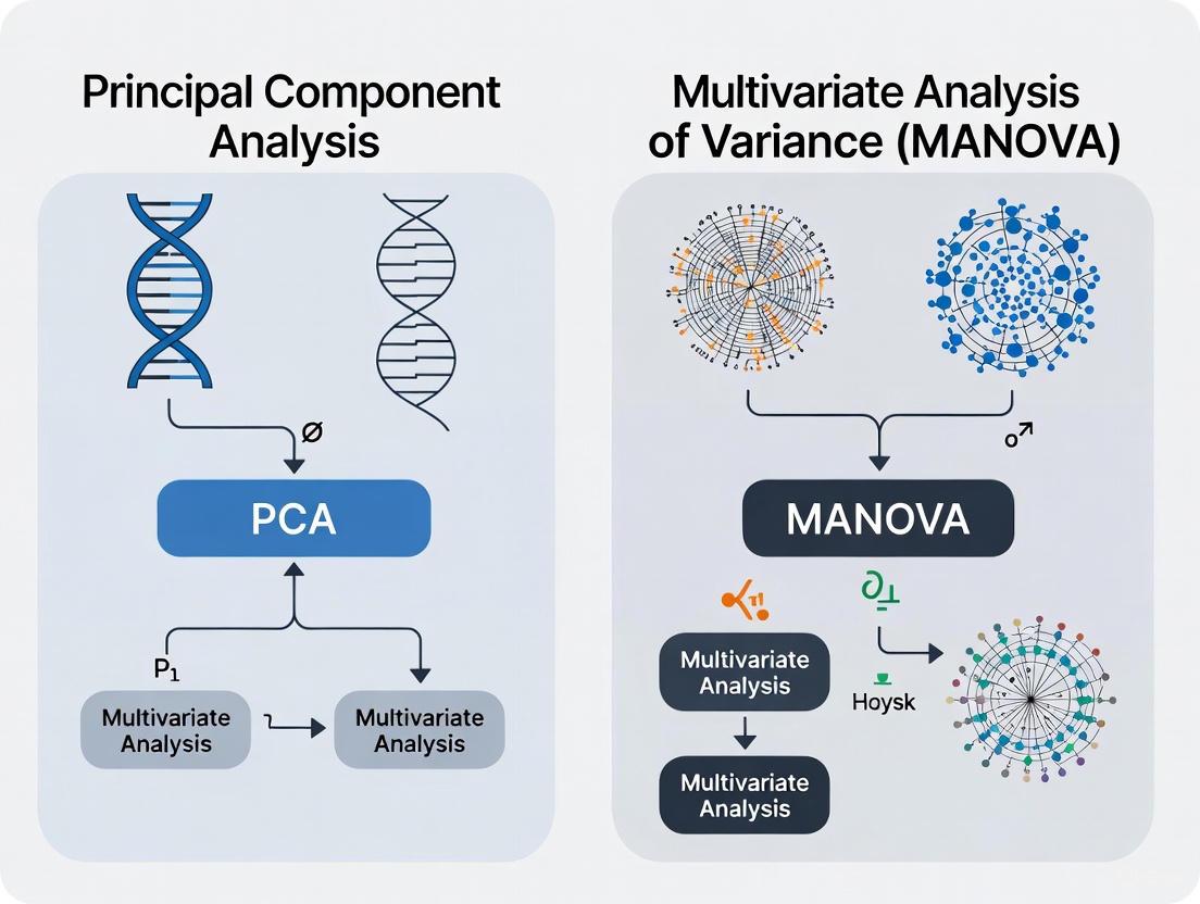
The relationship between exploratory and confirmatory analysis in genomic studies follows a logical progression that can be visualized as a workflow:

Figure 1: Integrated analytical workflow showing the complementary relationship between PCA and MANOVA in genomic studies.

This workflow illustrates how exploratory and confirmatory analyses are not in opposition but rather work together in a complementary fashion [7]. PCA helps generate hypotheses by revealing patterns in the data, while MANOVA formally tests these hypotheses using rigorous statistical frameworks.

Limitations, Considerations, and Alternative Approaches

5.1 Limitations of PCA PCA has several important limitations in gene expression analysis. It assumes linear relationships between variables, which may not capture complex biological interactions [2]. The technique is sensitive to sample composition; studies have shown that the specific principal components identified depend strongly on the sample distribution in the dataset [5]. When a dataset contains many samples from a particular tissue type, that tissue may dominate early principal components regardless of its biological significance. Additionally, PCA may fail to detect biologically relevant information embedded in higher-order components, particularly for tissue-specific information that remains in the residual space after subtracting the first three PCs [5].

5.2 Limitations of MANOVA MANOVA requires meeting several statistical assumptions that can be challenging with genomic data. The test assumes multivariate normality, homogeneity of covariance matrices, and independence of observations [3]. Violations of these assumptions can lead to inaccurate results. MANOVA also becomes increasingly complex to interpret with many dependent variables, and it provides an overall test of significance without immediately indicating which specific variables drive group differences.

5.3 Alternative and Complementary Methods Several alternative approaches address limitations of both PCA and MANOVA:

• Canonical Variates Analysis: Particularly effective for designed experiments with replicates, as it enhances group discrimination by keeping subjects belonging to the same group close together in the transformed space [8].

• t-Distributed Stochastic Neighbor Embedding: A nonlinear dimensionality reduction technique particularly effective for visualizing high-dimensional gene expression data and identifying clusters [9].

• PCA-Projected F-test: Combines the dimensionality reduction of PCA with rigorous statistical testing, providing better empirical power performance than classical MANOVA Wilks' Lambda-test in high-dimensional settings with small sample sizes [9].

Table 2: Research Reagent Solutions for Gene Expression Analysis

Reagent/Resource	Function in Analysis	Application Context
Affymetrix Microarray Platforms	Genome-wide expression profiling	Generating high-dimensional gene expression data [5]
R Statistical Software	Implementation of PCA, MANOVA, and related methods	Primary tool for statistical analysis and visualization [5] [6]
NCSS Multivariate Analysis Module	Commercial software for MANOVA, PCA, and other multivariate tests	User-friendly implementation of complex statistical models [1]
aomisc R Package	Provides Canonical Variates Analysis functions	Enhanced group discrimination for designed experiments [8]
vegan R Package	Community ecology package with ordination methods	PCA implementation and biodiversity analysis [8]

PCA and MANOVA serve distinct but complementary roles in high-dimensional gene expression analysis. PCA excels as an exploratory tool for visualizing data structure, identifying patterns, and reducing dimensionality, while MANOVA provides rigorous confirmatory testing for group differences across multiple outcome variables. The most effective analytical strategies employ both techniques sequentially: using PCA to generate hypotheses from complex genomic data, then applying MANOVA to formally test these hypotheses within a statistical framework. Understanding the strengths, limitations, and proper applications of each method enables researchers to draw more reliable biological conclusions from complex gene expression datasets, ultimately advancing drug development and genomic science.

In high-dimensional gene expression analysis, researchers are often faced with the challenge of extracting meaningful biological signals from datasets where the number of variables (genes) far exceeds the number of observations (samples). This "large p, small n" problem necessitates robust dimensionality reduction techniques that can uncover underlying patterns while managing computational complexity. Principal Component Analysis (PCA) and Multivariate Analysis of Variance (MANOVA) represent two fundamentally different approaches for handling multivariate data. This guide provides an objective comparison of these methodologies, examining their performance characteristics, statistical power, and practical applicability in genomic research to help scientists select the appropriate tool for their analytical needs.

Understanding the Core Methodologies

Principal Component Analysis (PCA): A Dimension Reduction Workhorse

PCA is an unsupervised dimensionality reduction technique that transforms high-dimensional data into a new coordinate system comprised of orthogonal principal components (PCs). These components are linear combinations of the original variables, ordered such that the first PC captures the maximum possible variance in the data, the second PC captures the next highest variance while being orthogonal to the first, and so on [10].

The mathematical foundation of PCA involves several key steps. First, the data is standardized to have zero mean and unit variance, ensuring that variables with larger scales do not disproportionately influence the results. Next, the covariance matrix is computed to capture the relationships between all pairs of variables. Eigen decomposition of this covariance matrix yields eigenvectors (which define the directions of the principal components) and eigenvalues (which represent the amount of variance explained by each component) [10]. The top k eigenvectors are selected based on their corresponding eigenvalues, effectively projecting the data onto a lower-dimensional subspace while preserving the maximal variance structure.

In genetic association studies, PCA has demonstrated particular utility for analyzing multiple correlated phenotypes. Contrary to widespread practice, research has shown that testing only the top PCs often has low power, whereas combining signals across all PCs can significantly improve power to detect genetic variants with opposite effects on positively correlated traits and variants exclusively associated with a single trait [11].

MANOVA: The Traditional Multivariate Approach

MANOVA represents the traditional multivariate generalization of ANOVA, designed to test for statistically significant differences between groups across multiple dependent variables simultaneously. The method tests whether the mean vectors of the groups are equal, while accounting for correlations between response variables [12]. MANOVA models the total variance-covariance matrix by partitioning it into components attributable to different experimental factors and their interactions, followed by hypothesis testing typically using statistics such as Wilks' Lambda, Pillai's Trace, or Hotelling's T².

However, MANOVA faces fundamental limitations when applied to high-dimensional biological data. The method has strict requirements for sample size, demanding more observations than variables—a condition rarely met in genomic studies where thousands of genes are measured across relatively few samples [12] [13]. This limitation arises from the need to estimate a full covariance matrix, which becomes singular when the number of variables exceeds the number of observations. Additionally, MANOVA assumes multivariate normality, homogeneity of covariance matrices, and independence of observations—assumptions frequently violated in high-throughput genomic data [12].

Direct Performance Comparison: PCA vs. MANOVA

Table 1: Methodological Comparison of PCA and MANOVA for High-Dimensional Data Analysis

Characteristic	PCA	MANOVA
Data Requirements	No strict sample size requirements	Requires more samples than variables
Dimensionality Handling	Excellent for high-dimensional data ("large p, small n")	Fails with high-dimensional data due to singular covariance matrices
Statistical Power	High when combining all components [11]	Limited with high-dimensional data
Implementation Complexity	Low; efficient algorithms available	High; requires regularization for high-dimensional data
Interpretability	Components may lack biological meaning	Direct group difference testing
Assumptions	Few assumptions beyond linearity	Multivariate normality, homogeneity of covariance matrices
Multiple Testing Burden	Reduced through dimension reduction	Severe without prior dimension reduction

Table 2: Experimental Performance Comparison Across Biological Data Types

Application Domain	PCA Performance	MANOVA Performance	Key Findings
Genetic Association Studies	Powerful for detecting pleiotropic variants [11]	Not directly applicable without modification	Combined-PC approach showed near-optimal power across scenarios
Imaging Genetics	Extensively used for brain endophenotype analysis [14]	Limited application due to high dimensionality	PCA enables multivariate analysis of correlated neuroimaging phenotypes
Metabolomics	ASCA (ANOVA-SCA) effectively handles designed experiments [12]	Requires regularization (rMANOVA)	All ANOVA-based methods detected significant factors, with similar performance
Multi-Source Data Integration	Enables integration through shared latent spaces [13]	Cannot directly handle distinct variable spaces	Bayesian multi-way models extend PCA concepts for multi-source data

Experimental Protocols and Validation

Protocol 1: Evaluating PCA Power in Genetic Association Studies

Objective: To assess the power of different PCA strategies for identifying genetic variants associated with multiple correlated traits.

Methodology:

• Data Generation: Simulate multiple positively correlated, normally distributed phenotypes (Y₁, Y₂, ..., Yₙ) with mean 0 and variance 1, influenced by an unknown variable U and a scaled genotype G (both normally distributed with mean 0 and variance 1).
• Trait Construction: Construct trait vectors using the model: Yᵢ = c∗u + √vᵢ∗g + √(1−c−vᵢ)∗εᵢ, where εᵢ denotes independent random noise normally distributed with mean 0 and variance 1 [11].
• PCA Implementation: Compute principal components of the trait correlation matrix, deriving both top-variance PCs and all PCs.
• Association Testing: Test associations between genotype G and (a) individual traits, (b) top PCs only, and (c) all PCs combined using joint tests.
• Power Calculation: Compute statistical power using noncentral chi-square distributions with appropriate degrees of freedom [11].

Key Findings: Analysis of up to 100 correlated traits demonstrated that testing only the top PCs often has low power, whereas combining signals across all PCs substantially improves power, particularly for detecting genetic variants with opposite effects on positively correlated traits and variants exclusively associated with a single trait [11].

Protocol 2: Comparing Multivariate Methods in Metabolomics

Objective: To evaluate the performance of ANOVA-based multivariate methods (ASCA, rMANOVA, GASCA) for determining significant experimental factors and relevant variables in metabolomic studies.

Methodology:

• Experimental Design: Generate two LC-MS datasets with different complexity: (1) yeast samples with two extraction protocols (single factor), and (2) zebrafish embryos exposed to two endocrine disruptor chemicals at two concentration levels (multiple factors) [12].
• Data Preprocessing: Process raw chromatograms to obtain total ion current (TIC) profiles and integrated peak areas.
• Method Application: Apply ASCA, rMANOVA, and GASCA to assess statistical significance of experimental factors using permutation tests (typically 10,000 permutations).
• Variable Selection: Identify relevant variables (potential markers) contributing most to factor effects.
• Validation: Compare results with standard methods (univariate tests, PLS-DA with VIP scores) to evaluate reliability [12].

Key Findings: All three ANOVA-based methods successfully detected statistically significant factors, with ASCA and rMANOVA producing p-values at the lower threshold of permutations. GASCA showed more variation between ionization modes but identified relevant variables that strongly aligned with those detected by PLS-DA, suggesting higher reliability for biomarker discovery [12].

Visualization of Analytical Workflows

PCA Workflow for High-Dimensional Biological Data

MANOVA Limitations and Modern Extensions

The Scientist's Toolkit: Essential Research Reagents and Computational Solutions

Table 3: Essential Research Reagents and Computational Tools for Multivariate Analysis

Tool/Resource	Type	Function	Application Context
R Statistical Environment	Software Platform	Comprehensive statistical computing and graphics	Implementation of PCA, MANOVA, and specialized packages for omics data
Python (scikit-learn, glycowork)	Programming Language	Machine learning and compositional data analysis	PCA implementation and specialized analysis pipelines for glycomics [15]
ASCA+ Toolkit	Chemometrics Package	ANOVA-simultaneous component analysis	Designed metabolomic studies with multiple experimental factors [12]
Multi-Way CCA	Bayesian Model	Multi-way, multi-source data integration	Integrated analysis of metabolic and gene expression profiles [13]
KernelDEEF	Computational Method	Completely data-driven profile comparison	Conversion of single-cell expression data to donor-by-feature matrices [16]
mAP Framework	Statistical Framework	Profile strength and similarity evaluation	Assessment of phenotypic activity in high-dimensional profiling data [17]

The comparative analysis reveals distinct advantages and limitations for both PCA and MANOVA in high-dimensional gene expression research. PCA emerges as the more versatile and practical approach for exploratory analysis and dimension reduction in typical "large p, small n" scenarios, while MANOVA and its modern extensions offer rigorous hypothesis testing frameworks when methodological assumptions can be satisfied.

For researchers designing genomic studies, the following evidence-based recommendations are provided:

• Prioritize PCA-based approaches for initial exploratory analysis of high-dimensional genomic data, particularly when sample sizes are limited relative to the number of variables measured.

• Implement combined-PC testing strategies rather than analyzing only top-variance components, as this approach maintains power to detect diverse genetic association patterns [11].

• Consider regularized MANOVA variants or ASCA when analyzing data from designed experiments with multiple factors, as these methods balance statistical rigor with practical applicability to high-dimensional data [12].

• Adopt multi-source integration methods when combining heterogeneous data types (e.g., transcriptomics and metabolomics), as these specialized techniques can reveal biological insights not apparent from single-source analyses [13].

The choice between PCA and MANOVA ultimately depends on specific research objectives, data characteristics, and analytical requirements. PCA excels in dimension reduction and pattern discovery, while MANOVA and its extensions provide formal statistical testing for experimental factors. Understanding these complementary strengths enables researchers to select optimal strategies for extracting meaningful biological insights from complex genomic datasets.

Multivariate Analysis of Variance (MANOVA) is a sophisticated statistical procedure used to determine whether there are statistically significant differences between the means of multiple groups across several dependent variables simultaneously. As an extension of Analysis of Variance (ANOVA), MANOVA allows researchers to analyze the effect of one or more independent variables on multiple continuous dependent variables while considering the interrelationships between these outcome measures. This multivariate technique is particularly valuable in complex research domains like genomics and drug development, where phenomena are typically influenced by multiple correlated outcome measures rather than isolated variables.

The fundamental principle behind MANOVA is its ability to combine multiple dependent variables into a weighted linear composite, creating a new "latent variate" upon which group differences are tested. This approach provides several advantages over conducting multiple ANOVAs, including enhanced statistical power for detecting specific patterns and better control over experiment-wise Type I error rates. In high-dimensional biological research, such as gene expression analysis, MANOVA offers a framework for understanding how experimental conditions collectively influence multiple molecular outcomes, providing a more holistic view of treatment effects than univariate methods.

Fundamental Concepts and Comparison with ANOVA

Core Differences Between MANOVA and ANOVA

MANOVA expands upon the traditional ANOVA framework by accommodating multiple dependent variables in a single analysis. While ANOVA assesses whether group means differ on a single outcome variable, MANOVA evaluates whether groups differ on a combination of several outcome measures. This fundamental distinction creates significant implications for research design, interpretation, and application across scientific domains.

Table 1: Key Differences Between ANOVA and MANOVA

Parameter	ANOVA	MANOVA
Full Name	Analysis of Variance	Multivariate Analysis of Variance
Dependent Variables	Single continuous dependent variable	Two or more continuous dependent variables
Objective	Determine differences in group means for one outcome	Determine independent variable effects on multiple outcomes and their interactions
Nature	Parametric	Multivariate parametric
Test Statistics	F-statistic	Wilks' Lambda, Pillai's Trace, Hotelling-Lawley Trace, Roy's Largest Root
Variance Assessment	Assesses ratio between group mean differences and within-group variance	Optimally combines variables to enhance group differences using variance-covariance
Error Rate Control	Individual test error rate	Controls experiment-wise error rate for multiple dependent variables

When to Choose MANOVA Over ANOVA

MANOVA provides particular advantages in specific research scenarios. It is ideally suited when dependent variables are moderately correlated conceptually or statistically, as the technique leverages these relationships to identify patterns that might remain hidden in separate univariate analyses. For example, in pharmaceutical research, MANOVA could simultaneously analyze how different drug formulations affect multiple efficacy endpoints (e.g., biomarker levels, symptom scores, functional measures) while accounting for their natural correlations.

The method offers greater statistical power when analyzing correlated dependent variables, enabling detection of smaller effects that might be missed by individual ANOVA tests. This advantage stems from MANOVA's ability to account for variance-covariance structures in the data. Additionally, by conducting one multivariate test instead of multiple univariate tests, researchers maintain better control over the family-wise error rate, reducing the likelihood of false positive findings when examining multiple outcome measures.

Mathematical Foundation of MANOVA

The MANOVA Model

The MANOVA procedure operates on the general linear model framework, expressed mathematically as:

Y = βX + ε

Where Y is an n × m matrix of dependent variables (n observations on m response variables), X is an n × p matrix of predictor variables, β is a p × m matrix of regression coefficients, and ε is an n × m matrix of residuals. This formulation extends the univariate general linear model to accommodate multiple response variables simultaneously.

The null hypothesis tested in MANOVA is:

H₀: μ₁ = μ₂ = ⋯ = μₖ

Where μᵢ represents the vector of means for the i-th group across all dependent variables. The alternative hypothesis states that at least one group mean vector differs from the others. MANOVA evaluates this hypothesis by partitioning the total variance-covariance matrix into between-groups and within-groups components, analogous to how ANOVA partitions sum of squares.

Test Statistics in MANOVA

MANOVA employs several test statistics to evaluate multivariate significance, each with particular strengths and applications:

• Wilks' Lambda (Λ) : The most commonly reported MANOVA statistic, calculated as the ratio of the determinant of the within-groups sum of squares and cross-products matrix to the determinant of the total sum of squares and cross-products matrix: Λ = |W|/|T| = |W|/|B + W|, where W is the within-group matrix and B is the between-group matrix. Smaller values of Wilks' Lambda indicate stronger evidence against the null hypothesis.

• Pillai's Trace : The sum of the explained variances of the discriminant functions, calculated as V = trace[B(T)⁻¹]. This statistic is generally more robust to violations of assumptions, particularly when sample sizes are small or homogeneity of covariance is questionable.

• Hotelling-Lawley Trace : The sum of the eigenvalues of the matrix BW⁻¹, representing the ratio of between-groups to within-groups variation. This statistic is useful when group sizes are unequal but assumptions are met.

• Roy's Largest Root : The largest eigenvalue of BW⁻¹, which tests only the first discriminant function. This statistic is most powerful when one dominant function separates groups but is sensitive to assumption violations.

Table 2: MANOVA Test Statistics and Their Formulas

Test Statistic	Formula	Interpretation
Wilks' Lambda	Λ = |W|/|T| = |W|/|B + W|	Smaller values indicate significant group differences
Pillai's Trace	V = trace[B(T)⁻¹]	More robust to assumption violations
Hotelling-Lawley Trace	U = trace(BW⁻¹)	Ratio of between to within-group variation
Roy's Largest Root	θ = λₘₐₓ(BW⁻¹)	Tests only the first and largest discriminant function

MANOVA in Gene Expression Analysis

Applications in Genomic Research

In high-dimensional gene expression analysis, MANOVA offers distinct advantages for detecting differentially expressed genes across multiple experimental conditions. Traditional approaches often summarize multiple probe-level measurements into single scores before conducting differential expression analysis, risking information loss and potentially reaching inaccurate conclusions. MANOVA addresses this limitation by simultaneously analyzing multiple probe-level measurements, preserving the multivariate nature of the data and potentially increasing detection power.

For oligonucleotide arrays like Affymetrix GeneChips, where multiple probes measure each gene's mRNA abundance, robustified MANOVA approaches have been developed specifically for detecting differentially expressed genes in both one-way and two-way experimental designs. These methods can be extended to identify special patterns of gene expression through profile analysis across multiple populations, utilizing probe-level data without restrictive distributional assumptions through permutation-based testing.

MANOVA vs. PCA in High-Dimensional Data

While both MANOVA and Principal Component Analysis (PCA) handle multivariate data, they serve distinct purposes in gene expression research. PCA is primarily a dimension-reduction technique that transforms correlated variables into a smaller set of uncorrelated principal components, capturing maximum variance in the data. In contrast, MANOVA is a group-comparison method that tests whether population means differ across multiple dependent variables.

In practice, these methods can be complementary. PCA might precede MANOVA to reduce dimensionality while preserving data structure, especially when dealing with thousands of genes where MANOVA would be computationally prohibitable. However, when focusing on specific gene sets or pathways, MANOVA directly tests experimental effects on multiple correlated expression measures, potentially detecting coordinated expression changes that would be missed in univariate analyses.

Figure 1: Comparative Workflow of PCA and MANOVA in Gene Expression Analysis

Experimental Design and Protocols

Implementing MANOVA in Gene Expression Studies

The application of MANOVA to gene expression data requires careful experimental design and execution. A typical protocol involves:

1. Probe-Level Data Preparation: Rather than summarizing probe-level data into single expression values, maintain multiple probe measurements as dependent variables. This preserves the multivariate nature of the data and allows MANOVA to detect patterns across probes.

2. Experimental Design Specification: For one-way MANOVA, different experimental conditions (e.g., treatment vs. control) serve as the grouping variable. For two-way MANOVA, multiple factors (e.g., treatment type and time point) can be incorporated with their interaction terms.

3. Assumption Checking: Verify multivariate normality using Mardia's test or Q-Q plots. Assess homogeneity of variance-covariance matrices using Box's M test (with significance set at α=.001 due to sensitivity). Check for multicollinearity among dependent variables, with correlations ideally below r=.90.

4. Robustified MANOVA Implementation: Apply permutation-based testing when distributional assumptions are violated, as implemented in robustified MANOVA packages specifically designed for gene expression data.

5. Interpretation and Follow-up: Upon finding significant multivariate effects, conduct appropriate post-hoc analyses to identify which specific genes and conditions contribute to the significant results, using methods like discriminant function analysis or protected univariate ANOVAs.

Research Reagent Solutions for MANOVA Experiments

Table 3: Essential Research Reagents and Materials for Gene Expression MANOVA Studies

Reagent/Material	Function in MANOVA Experiments
Affymetrix GeneChip Arrays	Platform for simultaneous measurement of multiple probe-level expressions for each gene
RNA Extraction Kits	Isolation of high-quality RNA for accurate gene expression measurement
cDNA Synthesis Kits	Reverse transcription of RNA to cDNA for hybridization to arrays
Hybridization Reagents	Facilitate binding of cDNA to array probes for accurate signal detection
Statistical Software (R, SPSS, SAS)	Implementation of MANOVA and robustified MANOVA procedures with permutation tests
Quantile Normalization Tools	Standardization of data distributions for assumption compliance

Assumptions and Methodological Considerations

Critical Assumptions for Valid MANOVA

MANOVA relies on several key assumptions that researchers must verify before interpreting results:

• Multivariate Normality: Each dependent variable should follow a normal distribution within groups. While MANOVA is somewhat robust to minor violations, severe non-normality can affect test validity. Transformation of variables or use of non-parametric alternatives may be necessary when this assumption is violated.

• Homogeneity of Variance-Covariance Matrices: The population variance-covariance matrices across groups should be equal. This multivariate extension of homogeneity of variance is tested using Box's M statistic, with violations potentially leading to inflated Type I error rates.

• Absence of Multicollinearity: Dependent variables should be moderately correlated but not too highly correlated (generally r < .90). Extreme multicollinearity can cause computational problems and interpretation difficulties.

• Independence of Observations: All cases should be independent of each other, with no systematic pattern in participant selection or data collection.

• Adequate Sample Size: Each group should contain more cases than the number of dependent variables, with larger samples improving power and robustness to assumption violations. A general guideline is N > (p + m), where N is sample size per group, p is number of dependent variables, and m is number of groups.

Addressing Common Challenges in Genomic Applications

High-dimensional gene expression data presents unique challenges for MANOVA implementation. When the number of genes (dependent variables) exceeds sample size, traditional MANOVA becomes infeasible due to rank deficiency in the variance-covariance matrix. In such cases, regularized MANOVA approaches or preliminary dimension reduction techniques like PCA may be employed.

For detecting differentially expressed genes, robustified MANOVA methods utilizing permutation tests offer advantages when distributional assumptions are questionable. These approaches have demonstrated superior performance in maintaining false discovery rates while increasing power compared to univariate methods, particularly when the number of experimental groups is small.

Comparative Performance in High-Dimensional Biology

Advantages of MANOVA in Detecting Multivariate Patterns

MANOVA offers several distinct advantages over univariate approaches in genomic and pharmaceutical research:

• Enhanced Pattern Detection: By considering multiple dependent variables simultaneously, MANOVA can identify treatment effects that manifest across combinations of variables rather than in individual measures. For example, a drug might not significantly affect individual biomarker levels but could produce a detectable pattern across multiple correlated biomarkers.

• Type I Error Control: When analyzing multiple outcome variables, conducting separate ANOVAs inflates the family-wise error rate. MANOVA maintains the experiment-wise error rate at the nominal level (e.g., α=.05) by testing all outcomes simultaneously.

• Increased Power for Correlated Outcomes: With moderately correlated dependent variables, MANOVA often demonstrates greater statistical power to detect group differences than separate univariate tests, particularly when group differences manifest in the covariance structure rather than in mean differences on individual variables.

Limitations and Alternative Approaches

Despite its advantages, MANOVA presents certain limitations that researchers should consider:

• Interpretation Complexity: Results from MANOVA can be more challenging to interpret than simple ANOVA findings, requiring understanding of multivariate statistics and potentially follow-up analyses.

• Sensitivity to Assumption Violations: MANOVA is generally more sensitive to violations of assumptions like multivariate normality and homogeneity of variance-covariance matrices than univariate ANOVA.

• Sample Size Demands: As the number of dependent variables increases, MANOVA requires larger sample sizes to maintain statistical power and validity.

• Limited Suitability for Ultra-High-Dimensional Data: In studies with thousands of genes, traditional MANOVA becomes computationally prohibitable, necessitating dimension reduction or regularized multivariate methods.

When MANOVA assumptions are severely violated or data dimensionality is extremely high, alternative approaches such as Regularized MANOVA, Distance-Based Methods (PERMANOVA), or Machine Learning Algorithms may be more appropriate for detecting multivariate group differences in gene expression data.

In the field of genomics, researchers frequently encounter a significant analytical challenge known as the "Large p, Small n" problem. This scenario occurs when the number of features or variables (p), such as genes, vastly exceeds the number of observations or samples (n). Gene expression studies from technologies like microarrays and RNA sequencing routinely generate data with tens of thousands of genes from only dozens or hundreds of samples, creating substantial statistical challenges for meaningful analysis. This dimensionality problem is particularly pronounced in single-cell RNA sequencing (scRNA-seq) data, where count matrices are "inherently high-dimensional and sparse" [18]. The analytical difficulties arising from this imbalance include increased risk of overfitting, where models memorize noise rather than learning true biological signals; reduced generalizability of findings; and computational inefficiencies. Furthermore, the presence of many irrelevant or redundant features can obscure the detection of genuinely important biological signals, complicating the identification of disease-relevant genes and pathways [19] [20].

Within this challenging landscape, dimensionality reduction techniques become essential tools for extracting meaningful biological insights. Among these, Principal Component Analysis (PCA) and Multivariate Analysis of Variance (MANOVA) represent two fundamentally different approaches to handling high-dimensional data. PCA operates as an unsupervised method that seeks to capture maximum data variance through linear combinations of the original variables, while MANOVA serves as a supervised technique for testing mean differences across groups across multiple response variables. The core challenge with MANOVA in high-dimensional settings is its fundamental requirement that the total sample size must be larger than the data dimension, a condition frequently violated in gene expression studies [9]. This article provides a comprehensive comparison of these methodological approaches within the context of gene expression analysis, examining their relative strengths, limitations, and appropriate applications for addressing the "Large p, Small n" challenge.

Analytical Framework: PCA versus MANOVA

Theoretical Foundations and Methodologies

Principal Component Analysis (PCA) is a cornerstone dimensionality reduction technique that transforms high-dimensional data into a new coordinate system comprised of orthogonal components that sequentially capture the maximum possible variance. The mathematical foundation of PCA relies on eigenvalue decomposition of the covariance matrix or singular value decomposition (SVD) of the data matrix. For a count matrix (X) with dimensions (m \times n) (where m represents cells and n represents genes), the SVD is expressed as (X = U\Sigma V^\top), where the principal components are derived from the columns of (V) [18]. PCA functions as an unsupervised method, meaning it does not utilize sample group labels in its dimensionality reduction process. This characteristic makes it particularly valuable for exploratory data analysis, visualization, and noise reduction before conducting formal statistical testing.

In contrast, Multivariate Analysis of Variance (MANOVA) represents a supervised statistical technique that extends ANOVA to handle multiple dependent variables simultaneously. The method tests the hypothesis that the population means of different groups are equal across multiple response variables, essentially examining whether group classifications explain a significant portion of the variance in the data. The classical MANOVA approach, particularly through tests like Wilks' Lambda, faces fundamental limitations in high-dimensional settings because it "requires a larger total sample size than the data dimension and mostly relies on an asymptotic null distribution" [9]. This requirement becomes problematic in gene expression studies where the number of genes (p) typically far exceeds the number of samples (n).

Comparative Performance in High-Dimensional Settings

Recent research has directly addressed the performance limitations of traditional MANOVA when applied to high-dimensional gene expression data. A novel methodology that combines t-SNE visualization with a PCA-projected exact F-test has demonstrated superior performance compared to classical MANOVA. In a Monte Carlo study, this projected F-test exhibited "better empirical power performance than the classical Wilks' Lambda-test" derived from MANOVA [9]. The key advantage of this approach lies in its accommodation of high-dimensional data with small sample sizes while maintaining an exact null distribution for the test statistic.

The following table summarizes the core methodological differences and performance characteristics of PCA, MANOVA, and the emerging hybrid approach:

Table 1: Comparison of Dimensionality Reduction and Testing Methods for High-Dimensional Gene Expression Data

Feature	PCA	Classical MANOVA	PCA-Projected F-test
Analysis Type	Unsupervised	Supervised	Supervised
Primary Function	Variance capture, dimensionality reduction	Multi-group mean comparison	Multi-group mean comparison
Sample Size Requirement	No strict minimum	Sample size > data dimension	Accommodates small sample sizes
Theoretical Basis	Eigenvalue decomposition, SVD	Likelihood ratio tests (e.g., Wilks' Lambda)	Exact F-distribution on projected data
High-Dimensional Performance	Effective for visualization, noise reduction	Performance degrades with high dimensionality	Maintains power in high dimensions
Key Limitation	Does not utilize group information	Relies on asymptotic distributions	Requires initial dimension reduction step

The superiority of the PCA-projected F-test approach stems from its two-step methodology: first employing dimension reduction (often through t-SNE or PCA) to visualize cluster structures, then applying rigorous statistical testing on the reduced space to validate differences between identified clusters. This integrated approach "bridges the gap between exploratory and confirmatory data analysis" while enhancing interpretability of complex gene expression data [9].

Experimental Protocols and Benchmarking Studies

Experimental Designs for Method Evaluation

Benchmarking studies for dimensionality reduction techniques typically employ carefully designed experiments using both labeled and unlabeled datasets with known ground truths. For labeled datasets, such as the Sorted PBMC Dataset (2,882 cells, 7,174 genes) and the 50/50 Jurkat:293T Cell Mixture Dataset (~3,400 cells), clustering accuracy is measured using the Hungarian algorithm and Mutual Information [18]. These metrics evaluate how well the dimensionality-reduced data preserves the known biological structure. For unlabeled datasets, internal validation metrics such as the Dunn Index and Gap Statistic assess cluster separation quality, while the Within-Cluster Sum of Squares (WCSS) quantifies variability preservation [18].

Experimental protocols typically involve applying multiple dimensionality reduction techniques to the same datasets and evaluating their performance across several criteria. For instance, studies have compared standard PCA (using full SVD), randomized SVD-based PCA, and Random Projection methods including Sparse Random Projection (SRP) and Gaussian Random Projection (GRP) [18]. The benchmarking process evaluates not only the computational efficiency but also the effectiveness in downstream analyses, particularly clustering performance and structure preservation.

Key Findings from Comparative Studies

Recent benchmarking studies have revealed several important insights regarding dimensionality reduction methods for high-dimensional gene expression data:

• Random Projection (RP) methods have demonstrated competitive performance compared to traditional PCA. In some evaluations, RP "not only surpasses PCA in computational speed but also rivals and, in some cases, exceeds PCA in preserving data variability and clustering quality" [18]. This is particularly valuable for large-scale scRNA-seq studies where computational efficiency is a practical concern.

• The projected F-test approach, which combines dimension reduction with rigorous statistical testing, has shown "better empirical power performance than the classical Wilks' Lambda-test" derived from MANOVA, especially in high-dimensional settings with small sample sizes [9].

• Alternative feature selection methods specifically designed for high-dimensional genetic data have emerged as valuable alternatives to pure dimension reduction. The copula entropy-based feature selection (CEFS+) approach, which captures full-order interaction gains between features, has demonstrated superior performance in classification tasks, particularly "on high-dimensional genetic datasets" [19].

• Knowledge-guided approaches that incorporate biological network information have shown promise in enhancing method performance. For example, the knowledge-slanted random forest integrates protein-protein interaction networks to modify feature selection probabilities, resulting in "improved precision in outcome prediction" compared to conventional methods, especially with very small sample sizes (n ≤ 30) [21].

The following workflow diagram illustrates the relationship between different analytical approaches for addressing the "Large p, Small n" challenge in gene expression studies:

Diagram 1: Analytical Approaches for Large p, Small n Data

Advanced Methodologies Addressing High-Dimensional Challenges

Feature Selection Innovations

Beyond conventional dimensionality reduction techniques, specialized feature selection methods have emerged as powerful alternatives for addressing the "Large p, Small n" challenge. Unlike dimension reduction that transforms features into new components, feature selection identifies informative subsets of original features, maintaining interpretability. The weighted Fisher score (WFISH) approach represents one such innovation that "assigns weights based on gene expression differences between classes" to prioritize biologically significant genes in high-dimensional classification problems [20]. When combined with random forest and k-nearest neighbors classifiers, WFISH has demonstrated lower classification errors compared to existing techniques across multiple benchmark datasets.

Another promising approach, copula entropy-based feature selection (CEFS+), employs a "maximum correlation minimum redundancy strategy for greedy selection" that specifically captures interaction gains between features [19]. This capability is particularly valuable in genomics, where "certain diseases are jointly determined by two or more genes" whose collective value exceeds their individual contributions. In comprehensive evaluations using three classifiers across five datasets, CEFS+ achieved the highest classification accuracy in 10 out of 15 scenarios, with particularly strong performance on high-dimensional genetic datasets.

Integrative Learning and Knowledge-Guided Approaches

Integrative learning represents a paradigm shift in addressing the small sample size problem by jointly analyzing multiple datasets containing the same set of variables. This approach "has the potential to mitigate the challenge of small n and large p" by enhancing the detection of weak yet important signals through aggregated information across studies [22]. The Structured Integrative Learning (SIL) framework further advances this concept by incorporating a priori known graphical structures of features, encouraging "joint selection of features that are connected in the graph" [22]. This integration of biological network information enhances statistical power while accounting for heterogeneity across datasets.

Knowledge-guided methods explicitly incorporate existing biological knowledge to improve analytical performance in high-dimensional settings. The knowledge-slanted random forest exemplifies this approach by using "biological networks as prior knowledge into the model to improve its performance and explainability" [21]. Through a random walk with restart algorithm on protein-protein interaction networks, this method modifies feature selection probabilities during random forest construction, resulting in improved prediction precision and identification of more biologically relevant genes, particularly in scenarios with very small sample sizes (n ≤ 30).

Table 2: Advanced Methodologies for Addressing the "Large p, Small n" Challenge

Methodology	Core Innovation	Advantages	Representative Applications
Projected F-test	Combines dimension reduction with exact F-test	Superior power to MANOVA; exact null distribution	Cluster validation in t-SNE plots [9]
Random Projection	Johnson-Lindenstrauss lemma for dimension reduction	Computational efficiency; preserves pairwise distances	Large-scale scRNA-seq analysis [18]
WFISH Feature Selection	Weighted differential expression scoring	Prioritizes biologically informative genes	Binary classification of tumor samples [20]
CEFS+ Feature Selection	Copula entropy with interaction capture	Identifies synergistic gene relationships	Disease classification from expression data [19]
Structured Integrative Learning	Multi-dataset analysis with graph information	Enhances weak signal detection; accounts for heterogeneity	Cross-study biomarker identification [22]
Knowledge-Slanted RF	Biological network-guided feature selection	Improved explainability; small sample performance	Disease-relevant gene identification [21]

Successfully navigating the "Large p, Small n" challenge requires both methodological sophistication and appropriate data resources. The following table outlines key reagents and resources essential for research in this domain:

Table 3: Essential Research Reagents and Resources for High-Dimensional Gene Expression Analysis

Resource Type	Specific Examples	Function and Application	Key Characteristics
Reference Datasets	GTEx (Genotype-Tissue Expression) [23]	Pan-tissue transcriptome analysis; benchmark studies	~17,000 transcriptomes across 54 tissues; age and sex metadata
Reference Datasets	Sorted PBMC Dataset [18]	Method benchmarking and validation	2,882 cells with 7 annotated cell populations
Biological Networks	Protein-Protein Interaction (PPI) Networks [21]	Prior knowledge for guided learning; pathway context	Encapsulates known functional relationships between genes
Software Tools	kslboruta R package [21]	Implementation of knowledge-slanted feature selection	Integrates PPI networks with random forest algorithm
Experimental Controls	Jurkat:293T Cell Mixture [18]	Technical validation of analytical pipelines	~3,400 cells with known 50:50 mixture ratio
Annotation Databases	Gene Ontology, KEGG Pathways [22]	Biological interpretation of results	Curated functional and pathway information

The "Large p, Small n" problem remains a fundamental challenge in gene expression studies, requiring sophisticated analytical approaches that balance statistical rigor with biological interpretability. While traditional methods like MANOVA face significant limitations in high-dimensional settings, emerging approaches such as the PCA-projected F-test offer superior performance for cluster validation by combining the variance-capturing capability of PCA with exact statistical testing. The continuing evolution of feature selection methods (WFISH, CEFS+) and knowledge-guided frameworks (Structured Integrative Learning, knowledge-slanted random forests) represents a promising direction for enhancing signal detection in small sample contexts while maintaining biological relevance.

For researchers navigating this landscape, the optimal strategy often involves selecting methods aligned with specific research objectives: dimension reduction techniques like PCA and random projection for visualization and noise reduction; projected testing approaches for rigorous hypothesis testing in high dimensions; advanced feature selection for identifying interpretable gene subsets; and integrative methods for boosting power through combined datasets. As the field advances, the integration of biological knowledge with statistical innovation will continue to drive progress in unraveling the complexity of gene expression data within the challenging "Large p, Small n" paradigm.

Principal Component Analysis (PCA) has established itself as a fundamental tool in the exploratory analysis of high-dimensional biological data, particularly in gene expression studies. As a dimensionality reduction technique, PCA transforms high-dimensional datasets into a new set of variables called principal components (PCs), which are linear combinations of the original features ordered by the amount of variance they explain. This transformation allows researchers to visualize the overall structure of complex datasets and identify patterns, clusters, and outliers that might otherwise remain hidden in thousands of dimensions. In the context of high-dimensional gene expression research, PCA provides unsupervised information on the dominant directions of highest variability, enabling investigators to compare these patterns with sample annotations or phenotypic information to detect previously unknown relationships or characterize poorly annotated samples.

The application of PCA extends beyond mere dimensionality reduction to critical quality assessment functions, including the detection of technical artifacts known as batch effects. These are systematic non-biological variations between groups of samples that result from experimental features not of biological interest, such as processing date, technician, or reagent batch. Left undetected, batch effects can confound biological interpretation and lead to spurious discoveries. PCA serves as a primary visual tool for determining whether batch effects exist after applying global normalization methods, allowing researchers to identify when samples cluster by technical rather than biological factors. When applying PCA to gene expression data, the standard approach involves computing principal components from a centered and scaled feature matrix, with the resulting components representing directions of maximum variance in the original data. The visualization of samples in the space defined by the first two principal components then provides a powerful overview of the major sources of variation across all samples and features.

Table 1: Core Dimensionality Reduction Techniques for Batch Effect Detection

Method	Input Data	Distance Measure	Primary Application	Batch Effect Detection Capability
PCA	Original feature matrix	Covariance/correlation matrix	Linear data, feature extraction	Moderate (may miss batch effects that aren't the largest variance source)
PCoA	Distance matrix	Various (Bray-Curtis, Jaccard, etc.)	Visualization of inter-sample relationships	Good (flexible distance measures can capture technical variations)
NMDS	Distance matrix	Rank-order relations	Complex datasets, nonlinear analysis	Good (preserves rank-order of sample relationships)
t-SNE/UMAP	Original feature matrix or distance matrix	Probability distributions	Visualization of complex structures	Excellent (can reveal subtle batch effects)

PCA Workflow for Batch Effect Identification

Standard PCA Protocol for Quality Assessment

Implementing PCA for batch effect identification requires a systematic workflow to ensure reliable detection of technical artifacts. The first step involves data preprocessing, where the feature data (typically a gene expression matrix with samples as columns and genes as rows) undergoes centering and scaling to ensure all features contribute equally regardless of their original measurement scale. This standardization is crucial when analyzing gene expression data where different genes may exhibit vastly different expression ranges. The computational implementation then involves singular value decomposition (SVD) of the preprocessed data matrix, which decomposes the data into orthogonal matrices that represent the principal components and their loadings. For modern omics datasets containing tens of thousands of features and hundreds of samples, specialized computational approaches are necessary to handle this scale efficiently.

The visualization phase involves projecting samples into the reduced dimensional space defined by the first few principal components, typically PC1 and PC2, which capture the largest proportion of variance in the dataset. In this visualization, each point represents a sample, and the spatial arrangement reveals similarities and differences between samples. Batch effects are identified when samples cluster according to technical factors such as processing date, sequencing batch, or laboratory technician rather than biological variables of interest. The interpretation requires careful examination of the principal component loadings to determine which features (genes) drive the separation between batches. This approach enables researchers to distinguish technical artifacts from true biological signals before proceeding with downstream analyses.

Limitations of Standard PCA and Guided PCA Approach

While standard PCA is valuable for initial data exploration, it possesses a critical limitation for batch effect detection: it identifies linear combinations of variables that contribute maximum variance, which means it may not detect batch effects if they are not the largest source of variability in the data. This limitation is particularly problematic in gene expression studies where strong biological signals (e.g., tissue type, disease status) often dominate the variance structure, potentially obscuring more subtle technical artifacts. Research has demonstrated that when batch effects are not the primary source of variation, traditional PCA methods do not work effectively for their detection, potentially leading to undetected technical confounding.

To address this limitation, guided PCA (gPCA) has been developed as an extension that specifically targets batch effect identification. Unlike standard unsupervised PCA, gPCA incorporates a batch indicator matrix into the analysis, guiding the singular value decomposition to explicitly look for batch effects in the data. The method produces a test statistic (δ) that quantifies the proportion of variance attributable to batch effects by comparing the variance of the first principal component from gPCA to that from unguided PCA. Large values of δ (approaching 1) indicate substantial batch effects, and statistical significance can be assessed through permutation testing. This approach provides a quantitative framework for batch effect detection that surpasses the visual inspection of standard PCA plots, offering greater sensitivity for identifying technical artifacts that might otherwise remain hidden beneath biological variation.

Table 2: Comparison of PCA Approaches for Batch Effect Detection

Feature	Standard PCA	Guided PCA (gPCA)
Objective	Identify directions of maximum variance	Specifically detect batch effects
Input	Feature matrix only	Feature matrix + batch indicator matrix
Detection Method	Visual inspection of PC plots	Quantitative test statistic (δ)
Sensitivity	Limited to largest variance sources	Targeted to batch effects regardless of magnitude
Output	Qualitative assessment	Quantitative p-value and effect size
Best Use Case	Initial exploratory analysis	Formal batch effect testing

Comparative Performance Evaluation: PCA Versus Alternative Methods

Multivariate Statistical Approaches

Beyond PCA, several multivariate statistical methods offer complementary approaches for batch effect detection and visualization. Principal Coordinate Analysis (PCoA) operates on a distance matrix rather than the original feature matrix, making it suitable for analyzing sample similarities using various distance measures such as Bray-Curtis or Jaccard indices. This flexibility allows PCoA to capture different nuances of interspecies relationships in microbial community studies or technical variations in gene expression datasets. Non-metric Multidimensional Scaling (NMDS) represents another distance-based approach that focuses on preserving the rank-order of sample relationships rather than absolute distances, making it particularly suitable for complex datasets with nonlinear structures where traditional PCA may underperform.

Recent research has introduced PERMANOVA (Permutational Analysis of Variance) as a powerful multivariate statistical test for batch effect evaluation. Studies comparing PERMANOVA to standard univariate testing methods have demonstrated its superior power in detecting batch effects across different sample sizes, with the Clark and Jaccard distance metrics showing particularly high sensitivity. Unlike traditional ANOVA, PERMANOVA does not assume normality or homogeneity of variances, making it suitable for the complex distributions often observed in genomic and radiomic features. When combined with effect size measures such as the Robust Effect Size Index (RESI), PERMANOVA provides both statistical significance testing and quantitative assessment of batch effect magnitude, addressing limitations of p-value-based approaches that become significant at extremely small effect sizes in large sample sizes.

Method Benchmarking and Performance Metrics

Comprehensive benchmarking studies have evaluated the performance of various batch effect detection and correction methods across different experimental scenarios. Quantitative assessments reveal that while PCA remains valuable for initial data exploration, it may be insufficient as a standalone method for comprehensive batch effect identification, particularly when technical artifacts are correlated with biological variables of interest. In comparative analyses, PERMANOVA has demonstrated higher power than standard univariate statistical tests across various sample sizes, with values of 0.952 and 1.0 at sample sizes of 100 and 2500 respectively when using Clark distance, compared to 0.812 and 0.991 for the best-performing univariate test (Anderson-Darling) at the same sample sizes.

The integration of multiple assessment methods creates a more robust framework for batch effect evaluation. A recommended pipeline employs PERMANOVA for initial dataset-level screening to identify the presence of batch effects, followed by RESI to quantify the effect size of batch at the feature level. This combined approach provides both statistical rigor and practical interpretability, enabling researchers to make informed decisions about whether and how to address batch effects in their data. Visual inspection methods like PCA and t-SNE complement these quantitative approaches by providing intuitive representations of data structure and batch-related clustering, creating a comprehensive assessment strategy that leverages the strengths of multiple methodologies.

PCA in the Context of MANOVA for High-Dimensional Data

Theoretical Foundations and Comparative Strengths

In high-dimensional gene expression analysis, researchers often face the choice between PCA and MANOVA (Multivariate Analysis of Variance) for exploring and testing multivariate group differences. While both methods handle multiple dependent variables simultaneously, they approach this task with fundamentally different objectives. PCA is an unsupervised dimension reduction technique that identifies the linear combinations of variables that explain maximum variance in the dataset without reference to group labels or experimental factors. In contrast, MANOVA is a supervised statistical test that evaluates whether population means on multiple dependent variables differ across groups defined by categorical independent variables.

The application of these methods to high-dimensional biological data reveals distinct advantages and limitations for each approach. PCA excels at exploratory analysis, providing visualization of overall data structure and revealing patterns that might not be hypothesized in advance. However, it lacks formal statistical testing framework for group differences. MANOVA offers rigorous hypothesis testing for group differences but becomes statistically problematic in high-dimensional settings where the number of variables exceeds the number of samples, a common scenario in genomics research. When comparing the two methods, PCA demonstrates greater utility for initial data quality assessment and batch effect detection, while MANOVA provides formal testing once batch effects have been addressed and biological hypotheses have been formulated.

Integrated Analytical Approaches

Rather than viewing PCA and MANOVA as competing methods, researchers can leverage them as complementary tools in a comprehensive analytical workflow. PCA serves as the first step for data quality assessment, identifying potential batch effects and outliers that might confound subsequent analyses. Once data quality issues have been addressed, MANOVA can test specific biological hypotheses about group differences in multivariate space. This sequential approach capitalizes on the strengths of both methods while mitigating their individual limitations.

Advanced hybrid methods have emerged that combine elements of both approaches. Principal Variance Component Analysis (PVCA) integrates the strengths of PCA and variance components analysis to quantify the contributions of different batch variables to overall variance in the dataset. This method provides a breakdown of key sources of variation, with unexplained variation classified as "residual." In ideal circumstances, the variation associated with known batch variables should be low and residual variation high, indicating minimal technical confounding. Similarly, guided PCA represents another hybrid approach that incorporates supervised elements (batch indicators) into the unsupervised PCA framework, creating a targeted method for batch effect detection that overcomes the limitation of standard PCA in detecting non-dominant variance sources.

Experimental Protocols and Implementation Guidelines

Standardized PCA Protocol for Batch Effect Detection

Implementing PCA for batch effect detection requires careful attention to methodological details to ensure reliable and reproducible results. The following protocol provides a standardized approach for gene expression datasets:

Sample Preparation and Data Generation: Process samples across multiple batches intentionally, ensuring that biological groups of interest are distributed across different batches when possible. For gene expression analysis, extract RNA and perform microarray or RNA-seq analysis following standard protocols, carefully documenting all technical parameters including processing date, technician, reagent lots, and instrument details.

Data Preprocessing: Format the data as a sample × gene matrix with expression values. For RNA-seq data, transform raw counts using variance-stabilizing transformation or log2(CPM + 1). Center and scale each gene to mean = 0 and standard deviation = 1 to ensure equal contribution of all genes regardless of expression level. Address missing values using appropriate imputation methods if necessary, though mean value imputation is commonly applied to centered data.

PCA Computation: Perform singular value decomposition (SVD) on the preprocessed data matrix using computational tools such as the prcomp() function in R or the PCA implementation in Python's scikit-learn. Retain all principal components initially for comprehensive assessment. Generate a scree plot showing the proportion of variance explained by each component to inform decisions about how many components to retain for further analysis.

Visualization and Interpretation: Create scatter plots of samples in the space defined by the first two principal components (PC1 vs. PC2) and subsequent component pairs (PC1 vs. PC3, PC2 vs. PC3). Color-code points according to potential batch variables (processing date, technician, etc.) and biological variables (disease status, tissue type, etc.). Interpret results by examining whether samples cluster more strongly by technical factors than biological factors, which indicates potential batch effects.

Research Reagent Solutions and Computational Tools

Table 3: Essential Research Reagents and Computational Tools for PCA-Based Batch Effect Analysis

Resource Category	Specific Tools/Reagents	Function/Purpose
Statistical Software	R Statistical Environment with packages (pcaMethods, sva, limma)	Primary computational platform for PCA and batch effect analysis
Python Libraries	scikit-learn, Scanpy, Scipy	Alternative computational environment for PCA implementation
Batch Correction Algorithms	ComBat, Harmony, Mutual Nearest Neighbors (MNN)	Correct identified batch effects while preserving biological variation
Visualization Tools	ggplot2, matplotlib, plotly	Create publication-quality visualizations of PCA results
Specialized Platforms	MetaBatch, CDIAM Multi-Omics Studio	Integrated web-based platforms for batch effect assessment
RNA Sequencing Kits	Illumina TruSeq, SMARTer Ultra Low Input	Generate gene expression data for analysis
Quality Control Reagents	Bioanalyzer RNA kits, Qubit quantification assays	Ensure input material quality before expression profiling

Advanced Applications and Future Directions

Integration with Other Omics Data Types

The application of PCA for batch effect detection has expanded beyond gene expression analysis to encompass diverse omics technologies, including metabolomics, proteomics, and radiomics. In metabolomics studies, platforms like MetaBatch have been developed specifically to assess and correct for batch effects in data from mass spectrometry and NMR spectroscopy. These implementations adapt the core PCA framework to address technology-specific challenges, such as the high proportion of missing values and strong analytical variation typical in metabolomic datasets. Similarly, in radiomics, where features are extracted from medical images, PCA and related multivariate methods help identify batch effects associated with different scanners, acquisition parameters, or reconstruction algorithms.

The growing importance of multi-omics integration presents both challenges and opportunities for PCA-based batch effect detection. When combining data from multiple omics platforms, batch effects can manifest both within and between technologies, creating complex confounding patterns. Advanced implementations of PCA can be applied to concatenated or integrated omics datasets to identify these complex batch effects, though specialized methods like Multi-Omics Factor Analysis (MOFA) may offer enhanced capability for cross-platform batch effect identification. As multi-omics studies become more prevalent, the development of integrated batch effect assessment pipelines that combine PCA with platform-specific quality metrics will become increasingly important for ensuring data quality and biological validity.

Emerging Methodologies and Best Practices

The field of batch effect detection and correction continues to evolve, with several emerging methodologies enhancing the capabilities of traditional PCA. The development of guided PCA (gPCA) represents a significant advancement that addresses the fundamental limitation of standard PCA in detecting batch effects that are not the largest source of variation. The gPCA approach provides a formal statistical test for batch effects, with a test statistic (δ) that quantifies the proportion of variance attributable to batch and a permutation-based approach for significance testing. This method offers improved sensitivity for detecting subtle batch effects that might be obscured by strong biological signals in standard PCA.

Recent research has also highlighted the importance of quantitative effect size measures alongside traditional p-value-based assessment. The Robust Effect Size Index (RESI) provides an interpretable metric for batch effect magnitude that remains meaningful at extremely large sample sizes where p-values become uninformative due to high sensitivity. The integration of RESI with PERMANOVA creates a comprehensive assessment framework that combines formal hypothesis testing with practical effect size quantification. As the field moves toward standardized reporting practices, the combination of visualization methods (PCA), statistical testing (gPCA, PERMANOVA), and effect size quantification (RESI) represents a best-practice approach for comprehensive batch effect assessment in high-dimensional biological data.

Future methodological developments will likely focus on addressing more complex batch effect scenarios, including nonlinear batch effects, sample-specific artifacts, and batch effects that interact with biological variables of interest. The integration of PCA with machine learning approaches may offer enhanced capability for detecting these complex patterns, while maintaining the interpretability that has made PCA a cornerstone of exploratory data analysis in biological research. As these methodologies mature, they will further solidify the role of PCA and related multivariate methods as essential tools for ensuring data quality and biological validity in high-dimensional genomic research.

A Step-by-Step Guide to Implementing PCA and MANOVA on Genomic Data

In high-dimensional gene expression analysis, the choice between statistical methods like Principal Component Analysis (PCA) and Multivariate Analysis of Variance (MANOVA) is profoundly influenced by data preprocessing decisions. Both techniques are fundamental for exploring and testing hypotheses in transcriptomic data, yet their effectiveness depends critically on proper normalization and standardization of the raw gene expression matrix. MANOVA tests for significant differences in mean vectors across groups, assuming homogeneity of covariance matrices, while PCA identifies dominant patterns of variation in the dataset, often driven by technical artifacts if not properly normalized. This guide provides an objective comparison of prevalent normalization methods, supported by experimental data, to inform reliable preprocessing for gene expression studies in pharmaceutical and basic research.

Normalization Methods for Gene Expression Data

Normalization adjusts for non-biological technical variations, such as sequencing depth and library composition, enabling meaningful biological comparisons. The following methods are commonly used, each with distinct approaches and implications for downstream analysis.

Method	Core Principle	Best Suited For	Key Assumptions
TMM (Trimmed Mean of M-values) [24] [25]	Scales library sizes based on a trimmed mean of log expression ratios (M-values) relative to a reference sample.	Between-sample comparison; differential expression analysis.	Most genes are not differentially expressed.
RLE (Relative Log Expression) [24] [26]	Calculates a scaling factor for a sample as the median of the ratios of its counts to the geometric mean across all samples.	Between-sample comparison; differential expression analysis.	Most genes are not differentially expressed.
GeTMM (Gene length corrected TMM) [24]	Combines gene length correction with the TMM method, reconciling within- and between-sample normalization.	Analyses requiring both within- and between-sample comparisons.	Similar to TMM, but also accounts for gene length.
TPM (Transcripts Per Million) [27] [25]	Normalizes for both sequencing depth and gene length within a sample. The sum of all TPMs is the same across samples.	Within-sample gene expression comparison.	Accounts for all technical variations within a single sample.
FPKM (Fragments Per Kilobase Million) [27] [25]	Analogous to TPM but fragments are used for paired-end data. Normalizes for sequencing depth and gene length.	Within-sample gene expression comparison (paired-end data).	Accounts for all technical variations within a single sample.
NORMA-Gene [28]	An algorithm-only method that uses least-squares regression on multiple target genes, eliminating the need for stable reference genes.	RT-qPCR studies; situations where validated reference genes are unavailable.	A normalization factor can be calculated from the expression of several genes to reduce variation.
Quantile Normalization [25]	Forces the distribution of gene expression values to be identical across all samples.	Making sample distributions comparable; microarrays and RNA-seq data.	The overall distribution of gene expression should be similar across samples.

The Impact of Normalization on MANOVA and PCA

The choice of normalization method directly affects the covariance structure of the data, which is a foundational element for both MANOVA and PCA.

• For MANOVA, the test assumes homogeneity of covariance matrices across groups. Improper normalization can introduce technical variances that differ between groups, violating this assumption and leading to inflated type I or type II errors. Between-sample normalization methods like TMM and RLE help maintain this homogeneity by controlling for library size differences that could systematically vary between experimental conditions.
• For PCA, the goal is to capture directions of maximum variance. Without proper normalization, the first principal components often represent dominant technical artifacts (e.g., differences in total read count) rather than biological signal. Methods like TMM and RLE are designed to mitigate these artifacts, ensuring that the leading PCs reflect biologically meaningful variation. In contrast, within-sample methods like TPM and FPKM are not sufficient for this purpose between samples, as they do not adequately control for compositional effects [27] [25].

Comparative Performance in Experimental Studies

Benchmarking Normalization for Genome-Scale Metabolic Models (GEMs)

A 2024 benchmark study evaluated five RNA-seq normalization methods—RLE, TMM, GeTMM, TPM, and FPKM—for their performance in building context-specific genome-scale metabolic models (GEMs) using iMAT and INIT algorithms for Alzheimer's disease (AD) and lung adenocarcinoma (LUAD) [24]. The study measured the variability in the number of active reactions in personalized models and the accuracy in capturing known disease-associated genes.

Table 1: Performance of Normalization Methods in Genome-Scale Metabolic Modeling

Normalization Method	Type	Variability in Model Size (Number of Active Reactions)	Accuracy in Capturing AD-Associated Genes	Accuracy in Capturing LUAD-Associated Genes
RLE	Between-sample	Low	~0.80	~0.67
TMM	Between-sample	Low	~0.80	~0.67
GeTMM	Between-sample	Low	~0.80	~0.67
TPM	Within-sample	High	Lower than between-sample methods	Lower than between-sample methods
FPKM	Within-sample	High	Lower than between-sample methods	Lower than between-sample methods

Experimental Protocol [24]:

• Data Collection: RNA-seq data from the ROSMAP cohort (for AD) and TCGA (for LUAD) were used.
• Normalization: The count data for each dataset were normalized using RLE (DESeq2), TMM (edgeR), GeTMM, TPM, and FPKM methods.
• Covariate Adjustment: Covariates like age, gender, and post-mortem interval (for AD) were regressed out from the normalized data.
• Model Building: Personalized metabolic models for each sample were generated using the iMAT algorithm mapped onto a human GEM.
• Evaluation:
  • Variability: The range in the number of reactions identified as active across individual models was assessed.
  • Accuracy: The models were evaluated based on their ability to correctly classify samples as disease or control, and the accuracy was calculated by comparing the identified disease-associated reactions to known metabolic genes for AD and LUAD.

Conclusion: Between-sample normalization methods (RLE, TMM, GeTMM) produced more robust and reproducible metabolic models with lower variability and higher accuracy than within-sample methods (TPM, FPKM). The performance of TPM and FPKM was improved after covariate adjustment, but their variability remained high [24].

Comparison for RT-qPCR Data: Reference Genes vs. NORMA-Gene

A 2025 study on sheep liver tissue compared normalization using multiple stable reference genes (HPRT1, HSP90AA1, B2M) with the NORMA-Gene algorithm for RT-qPCR data analyzing oxidative stress genes [28].

Table 2: Comparison of Normalization Methods for RT-qPCR

Normalization Method	Resources Required	Interpretation of GPX3 Expression	Effectiveness in Reducing Variance
Reference Genes (HPRT1, HSP90AA1, B2M)	High (Requires validation and running additional assays)	Significant effect of treatment observed	Less effective than NORMA-Gene
NORMA-Gene (Algorithm-only)	Low (No reference gene assays needed)	No significant effect of treatment observed	Better at reducing variance in target gene expression

Experimental Protocol [28]:

• Sample Collection: Liver samples from 34 sheep subjected to three different dietary treatments (maintenance, above maintenance, below maintenance).
• RNA Extraction and cDNA Synthesis: Total RNA was extracted, treated with DNase, and reverse transcribed.
• qPCR: Nine candidate reference genes and five target genes (CAT, GPX1, GPX3, PRDX1, SOD1) were amplified.
• Gene Stability Analysis: The stability of the nine reference genes was assessed using algorithms like geNorm and NormFinder to select the three most stable ones (HPRT1, HSP90AA1, B2M).
• Normalization:
  • The target gene expression was normalized using the geometric mean of the three stable reference genes.
  • The same expression data was normalized using the NORMA-Gene algorithm.
• Comparison: The effect of dietary treatment on each target gene was interpreted using both normalization methods, and the variance in normalized expression data was compared.

Conclusion: NORMA-Gene provided a more reliable normalization method that required fewer resources and was better at reducing variance, although it led to a different biological interpretation for one key gene (GPX3) [28].

A Novel Approach: Stable Combinations of Non-Stable Genes

Challenging the conventional paradigm of using individually stable genes, a 2024 study proposed a novel method that identifies a stable combination of non-stable genes for RT-qPCR normalization [29]. This method uses a comprehensive RNA-seq database to find a fixed number of genes whose individual expression values balance each other out across all experimental conditions of interest.

Experimental Workflow [29]:

• Database Selection: A comprehensive RNA-seq database (e.g., TomExpress for tomato) encompassing a wide range of biological conditions is used.
• Target Gene Mean Calculation: The mean expression level of the target gene is calculated from the RNA-seq data.
• Candidate Gene Pool: A pool of 500 genes with mean expressions similar to or greater than the target gene is selected.
• Combination Search: All possible combinations of k genes (e.g., k=3) from this pool are evaluated.
• Optimal Combination Selection: The optimal combination is selected based on two criteria:
  • The geometric mean of the k-gene combination has a mean expression greater than or equal to the target gene.
  • The arithmetic mean of the k-gene combination has the lowest possible variance across all conditions.
• Validation: The selected gene combination is validated against classic housekeeping genes and lowest variance genes using qPCR data.

Conclusion: This method demonstrated that a carefully selected combination of non-stable genes could outperform standard reference genes, including classical housekeeping genes and individually stable genes identified from RNA-seq data [29].

The Scientist's Toolkit: Key Reagents and Software

Table 3: Essential Research Reagents and Computational Tools

Item	Function/Application	Example Tools/Assays
RNA Extraction & QC	Isolate high-quality RNA for downstream transcriptomic analysis.	QIAzol Lysis Reagent, NanoDrop for purity/concentration check.
DNase Treatment	Remove genomic DNA contamination from RNA samples.	RQ1 RNase-Free DNase.
Reverse Transcription	Synthesize complementary DNA (cDNA) from RNA templates.	Reverse transcriptase enzymes.
qPCR Assays	Quantify gene expression with specific primers.	Primer pairs designed with Primer BLAST, SYBR Green chemistry.
Stable Reference Genes	Normalize RT-qPCR data; require experimental validation.	HPRT1, HSP90AA1, B2M (for sheep liver) [28].
RNA-seq Aligner	Map sequencing reads to a reference genome/transcriptome.	STAR, TopHat2, HISAT2.
Quantification Software	Generate raw count or TPM/FPKM expression estimates.	RSEM, Salmon, kallisto.
Normalization Packages	Implement between-sample normalization methods in R/Python.	edgeR (TMM), DESeq2 (RLE).
Batch Effect Correction	Remove technical variation across datasets/batches.	ComBat, Limma's removeBatchEffect.

Workflow and Decision Pathway

The following diagram illustrates a generalized workflow for preprocessing a gene expression matrix, highlighting key decision points for choosing a normalization strategy based on the data type and analytical goals.

The selection of a normalization method is a critical step that directly shapes the results of downstream analyses like PCA and MANOVA. Empirical evidence consistently shows that between-sample normalization methods (TMM, RLE, GeTMM) outperform within-sample methods (TPM, FPKM) for cross-sample comparisons in RNA-seq data, producing more robust and accurate biological models [24]. For RT-qPCR, algorithmic approaches like NORMA-Gene offer a resource-efficient and effective alternative to traditional reference genes [28]. Emerging methods, such as using stable combinations of genes identified from large RNA-seq databases, further push the boundaries of normalization accuracy [29]. Researchers must align their normalization strategy with their data type and analytical objectives to ensure the technical artifacts are minimized and the true biological signal is preserved for both exploratory (PCA) and hypothesis-testing (MANOVA) frameworks.

In high-dimensional gene expression analysis, researchers routinely face the challenge of extracting meaningful biological signals from datasets where the number of variables (genes) vastly exceeds the number of observations (samples). Principal Component Analysis (PCA) and Multivariate Analysis of Variance (MANOVA) represent two powerful statistical approaches with distinct philosophical frameworks and computational implementations for handling such data. PCA operates as an unsupervised dimension-reduction technique, transforming correlated variables into a set of uncorrelated principal components that capture maximum variance within the dataset. In contrast, MANOVA functions as a supervised hypothesis-testing method that evaluates whether group means differ significantly across multiple dependent variables simultaneously. The strategic application of these methods enables researchers to address fundamental questions in transcriptomics, from exploratory data visualization to confirmatory testing of experimental treatments.

Within genomic research, PCA has become indispensable for quality control, batch effect detection, and exploratory pattern recognition. By projecting high-dimensional gene expression data onto a reduced subspace defined by orthogonal principal components, researchers can visualize global sample relationships, identify potential outliers, and detect underlying structures that might correspond to biological or technical factors. Meanwhile, MANOVA offers a framework for testing specific hypotheses about how experimental conditions influence multiple gene expression patterns simultaneously, while controlling Type I error rates that would be inflated through repeated univariate testing. The complementary strengths of these methods make them valuable tools for comprehensive genomic analysis, each contributing unique insights into the complex architecture of gene regulation and expression.

Theoretical Foundations: PCA vs. MANOVA

Mathematical Framework of PCA

Principal Component Analysis begins with a data matrix X of dimensions ( n \times p ), where ( n ) represents the number of samples and ( p ) the number of genes. The first step involves centering the data by subtracting the mean of each variable, and often scaling to unit variance, creating matrix X_c. The core computational operation involves calculating the covariance matrix C = (\frac{1}{n-1})X_c^TX_c, which captures the relationships between all pairs of genes [30]. The principal components are then derived through eigen decomposition of C, satisfying the equation C = VΛV^T, where Λ is a diagonal matrix of eigenvalues (λ₁ ≥ λ₂ ≥ ... ≥ λ_p) representing the variance explained by each component, and V contains the corresponding eigenvectors that define the directions of maximum variance [30]. These eigenvectors are orthogonal unit vectors, ensuring the resulting components are uncorrelated.

The resulting principal components are linear combinations of the original genes, computed as T = X_cV, where T represents the scores matrix containing the coordinates of samples in the new principal component space. The proportion of total variance explained by the k-th principal component is calculated as λ_k/Σλ_i. In practice, the singular value decomposition (SVD) approach is often preferred for computational efficiency, particularly for datasets where ( p \gg n ), as it avoids explicit calculation of the large covariance matrix [30].

Mathematical Framework of MANOVA

MANOVA extends univariate ANOVA to multiple dependent variables by testing whether the centroids (multivariate means) of different groups differ significantly. The model for one-way MANOVA with g groups and n total observations can be expressed as Y_ij = μ + τ_i + ε_ij, where Y_ij is the vector of responses for the j-th subject in the i-th group, μ is the overall mean vector, τ_i represents the treatment effect for the i-th group, and ε_ij is the random error vector assumed to follow a multivariate normal distribution with mean zero and covariance matrix Σ [6].

The MANOVA hypothesis test evaluates H₀: τ₁ = τ₂ = ... = τ_g = 0 versus H₁: at least one τ_i ≠ 0. To test this hypothesis, MANOVA constructs two matrices: the hypothesis sum of squares and cross products (H) and the error sum of squares and cross products (E). Several test statistics are derived from these matrices, including Wilks' Lambda (Λ = |E|/|H+E|), Pillai's trace, Hotelling-Lawley trace, and Roy's largest root, each with different power characteristics under various alternative hypothesis scenarios [6].

Comparative Theoretical Strengths and Limitations

Table: Theoretical Comparison of PCA and MANOVA

Feature	PCA	MANOVA
Primary Objective	Dimension reduction, visualization, exploratory analysis	Hypothesis testing, group difference detection
Data Structure	Unsupervised, no grouping required	Supervised, requires predefined groups
Variance Modeling	Maximizes captured variance in entire dataset	Partitions variance into between-group and within-group components
Output	Principal components (linear combinations), variance explained	Test statistics (e.g., Wilks' Lambda), p-values
Data Distribution	No strict distributional assumptions	Assumes multivariate normality and homogeneity of covariance matrices
High-Dimensional Data	Computationally efficient via SVD	Requires more observations than variables; problematic for p > n
Multiple Testing	Not applicable	Controls experiment-wise error rate for multiple dependent variables

PCA's strength lies in its ability to simplify complex datasets by creating orthogonal components that capture the dominant patterns of variation, making it particularly valuable for initial data exploration in high-dimensional genomic studies [30]. However, PCA does not incorporate group information and may not highlight patterns relevant to specific research hypotheses. MANOVA explicitly tests group differences while accounting for correlations among multiple dependent variables, providing protection against inflated Type I errors that would occur with multiple ANOVAs [6]. Nevertheless, MANOVA struggles with high-dimensional data where the number of variables exceeds sample size, and violations of its distributional assumptions can compromise validity.

Experimental Protocols for Genomic Analysis

Protocol 1: PCA for Transcriptomic Data Exploration

Objective: To identify major sources of variation and potential sample outliers in RNA-seq data.

Step-by-Step Procedure:

• Data Preprocessing: Begin with normalized count data (e.g., TPM, FPKM, or variance-stabilized counts). Filter genes to exclude low-expression features, typically retaining those with counts >10 in at least 10% of samples. Log2-transform the data to stabilize variance [31].

• Gene Selection: For ultra-high-dimensional data, subset to the most variable genes to enhance signal detection. A common approach selects the top 500-1000 most variable genes based on median absolute deviation or variance [31]. This focuses the analysis on genes most likely to contribute to biological heterogeneity.

• Data Scaling: Center the data by subtracting the mean expression of each gene and scale to unit variance. Scaling prevents highly expressed genes from dominating the analysis simply due to their magnitude [30].

• Covariance Matrix Computation: Calculate the covariance matrix C of dimensions ( p \times p ) where ( p ) represents the number of selected genes. For very large p, this step can be computationally intensive but forms the foundation for principal component extraction [30].

• Eigen Decomposition: Perform eigen decomposition of C to obtain eigenvalues and eigenvectors. The eigenvalues represent the variance captured by each component, while eigenvectors (loadings) define the linear combinations of genes that form each principal component [30].

• Component Selection: Determine the number of meaningful components to retain. Common approaches include the elbow method using a scree plot, retaining components explaining >80% cumulative variance, or parallel analysis [30].

• Result Interpretation: Examine component loadings to identify genes contributing most to each component. Visualize sample relationships through biplots that overlay both sample positions (scores) and gene contributions (loadings).

Troubleshooting Tips: If the first component captures nearly all variance, investigate potential batch effects or technical artifacts. When biological signal appears weak, experiment with different gene selection thresholds or normalization approaches.

Protocol 2: MANOVA for Differential Expression Analysis

Objective: To test whether experimental groups show significant differences in multivariate gene expression patterns.

Step-by-Step Procedure:

• Data Preparation: Begin with normalized expression data for a predefined gene set. This might include genes within a pathway, co-expression module, or candidate gene panel. The number of genes should be substantially smaller than the sample size to avoid overfitting [14].

• Preliminary Assumption Checking:

  • Multivariate normality: Assess using Mardia's test or graphical methods like Q-Q plots
  • Homogeneity of covariance matrices: Evaluate using Box's M test
  • Multicollinearity: Check variance inflation factors among genes
  • Outliers: Identify using Mahalanobis distance [6]

• MANOVA Model Specification: Construct the model with the multivariate response matrix Y (samples × genes) and group membership as the independent variable. For single-factor designs, use the model: Y = μ + τ_i + ε_ij [6].

• Test Statistic Selection: Choose an appropriate test statistic based on study design and covariance heterogeneity:

  • Wilks' Lambda: General-purpose, most commonly used
  • Pillai's trace: More robust when covariance matrices are unequal
  • Hotelling-Lawley trace: Higher power when assumptions are met
  • Roy's largest root: Most powerful when groups separate along one dimension [6]

• Significance Testing: Calculate the test statistic and obtain p-values through F-approximation or permutation testing (recommended when assumptions are violated or sample size is small).

• Post-hoc Analysis: If the overall MANOVA is significant, conduct follow-up analyses to identify which genes contribute to group differences. Options include univariate ANOVAs with appropriate multiple testing correction, discriminant analysis, or inspection of canonical variates.

Troubleshooting Tips: For violated assumptions, consider applying transformations to the response variables, using more robust test statistics, or employing permutation tests. When the number of genes approaches sample size, consider dimension reduction as a preliminary step.

MANOVA Analysis Workflow for Genomic Data

Comparative Performance in Genomic Applications

Case Study 1: Sugarcane Quality Parameter Analysis

A comprehensive comparison of PCA and MANOVA was demonstrated in a study examining the impact of pre-harvest wilting treatments on sugarcane quality parameters [6]. Researchers applied both techniques to analyze measurements including Brix, Pol, fiber content, and juice purity across five treatment groups with four replications each.

Experimental Design: The study implemented a completely randomized block design with five wilting treatments (90, 75, 60, 45, and 30 days before harvest) applied to the CC-8592 sugarcane variety. For each treatment, researchers collected data on agronomic traits (weight, stem diameter, height) and quality parameters (Brix, Pol, purity) following standardized laboratory protocols [6].

PCA Findings: The PCA biplot revealed a strong correlation between quality variables (Brix, Pol, and juice purity), with the first two principal components accounting for 98.5% of the cumulative variance. This indicated a significant interrelation among these sucrose-related parameters in defining overall cane quality. The visualization showed that while fiber content was inversely correlated with purity, the wilting treatments did not form distinct clusters in the principal component space [6].

MANOVA Results: The MANOVA biplot analysis confirmed the PCA findings statistically, showing no significant differences among the wilting treatments across the multivariate quality metrics. This indicated that pre-harvest wilting time did not substantially alter these core quality parameters under the studied conditions, suggesting that other agronomic practices might have greater influence on sugarcane quality [6].

Table: Performance Comparison in Sugarcane Quality Study

Analysis Aspect	PCA Results	MANOVA Results	Interpretation
Treatment Separation	No clear clustering of treatments in PC space	No significant group differences (p > 0.05)	Wilting time does not affect quality
Variable Relationships	Strong correlation between Brix, Pol, purity	Not directly assessed	Quality parameters measure related traits
Variance Explanation	98.5% cumulative variance in first 2 PCs	Not applicable	Most variation in quality captured by two dimensions
Key Findings	Inverse relationship between moisture and purity	Wilks' Lambda non-significant	Consistent conclusion across methods

Case Study 2: High-Dimensional Transcriptome Analysis

In pan-tissue transcriptome analysis examining sex-dimorphic human aging, researchers systematically analyzed approximately 17,000 transcriptomes from 35 human tissues to evaluate how sex and age contribute to transcriptomic variations [23]. This large-scale genomic application highlights the complementary roles of dimension reduction and multivariate testing.

PCA Implementation: The researchers performed principal component analysis on both gene expression and alternative splicing data across multiple tissues. They developed a method called principal component-based signal-to-variation ratio (pcSVR) to quantify the distance between different sex or age groups divided by data dispersion within each group. This approach provided a global measurement of sex or age effects on transcriptomic variations by considering variations from all genes and AS events between different groups [23].

Key Findings: The PCA revealed that age showed substantially larger effects than sex on human transcriptome in most tissues for both gene expression and alternative splicing profiles. Interestingly, alternative splicing was significantly affected by both sex and age across most tissues, while gene expression was affected by sex in a much smaller number of tissues. Breakpoint analysis further showed that sex-dimorphic aging rates were significantly associated with decline of sex hormones, with males having a larger and earlier transcriptome change [23].

Methodological Insight: This study demonstrates how PCA-derived metrics can be adapted for specific research questions in high-dimensional genomic data. The pcSVR method effectively quantified group differences while handling the ultra-high dimensionality of transcriptome-wide data, an approach that would be challenging with traditional MANOVA due to the p > n problem [23].

Integration Strategies and Advanced Applications

Sequential Application of PCA and MANOVA

For high-dimensional genomic data where traditional MANOVA is mathematically impossible due to having more variables than observations, a sequential approach combining both methods offers a powerful solution:

• Dimension Reduction with PCA: First apply PCA to the complete gene expression dataset to reduce dimensionality. Retain the first k principal components that capture a substantial proportion of total variance (typically 70-90%) [11].

• MANOVA on Principal Components: Use the principal component scores as input variables for MANOVA testing of group differences. This approach respects the MANOVA requirement of having fewer variables than observations while preserving the multivariate nature of the analysis.

• Interpretation of Results: Significant MANOVA results indicate that groups differ in their positions within the multivariate space defined by the major patterns of variation in the gene expression data.

This combined approach was effectively demonstrated in a study of learning approaches in health science students, where researchers used MANOVA biplot to graphically represent relationships between learning approaches while testing for differences based on geographical origin [32].

Advanced PCA Variations for Genomic Data

Several specialized PCA implementations have been developed to address specific challenges in genomic analysis:

Sparse PCA: Incorporates regularization to produce principal components with sparse loadings, enhancing biological interpretability by focusing on smaller subsets of genes [30]. This approach is particularly valuable for identifying driver genes in expression patterns.

Supervised PCA: Incorporates outcome information to guide the dimension reduction process, potentially increasing relevance for subsequent predictive modeling [30]. This method can enhance power for detecting expression patterns associated with clinical outcomes.

Kernel PCA: Applies kernel methods to capture nonlinear relationships in gene expression data, potentially revealing complex patterns that linear PCA might miss [16].

Functional PCA: Adapted for time-course gene expression data, modeling trajectories rather than static measurements [30].

Advanced PCA Methods for Genomic Data

Research Reagent Solutions for Genomic Applications

Table: Essential Research Reagents and Computational Tools

Resource Category	Specific Tools/Packages	Primary Function	Application Context
Statistical Software	R (prcomp, factominer), SAS (PRINCOMP), MATLAB (princomp)	PCA implementation and visualization	General multivariate analysis of expression data
Specialized Packages	MultiPhen, PLINK, FactoMineR	Multivariate phenotype analysis	MANOVA and related methods for genomic data
Visualization Tools	ggplot2, plotly, biplot generators	Result presentation and interpretation	Creating publication-quality figures
Normalization Methods	DESeq2, edgeR, limma-voom	Data preprocessing for RNA-seq	Essential preparation step before PCA/MANOVA
High-Performance Computing	Parallel processing, cloud computing	Handling large genomic datasets	Managing computational demands of high-dimensional data

The comparative analysis of PCA and MANOVA reveals their complementary roles in high-dimensional gene expression research. PCA excels as an exploratory tool for visualizing data structure, detecting outliers, and reducing dimensionality, making it invaluable for initial data interrogation in studies with large feature spaces. MANOVA provides rigorous hypothesis testing for group differences across multiple correlated outcomes, controlling experiment-wise error rates while acknowledging the multivariate nature of biological systems.

The choice between these methods depends fundamentally on research objectives: PCA for unsupervised exploration of dominant variation patterns, MANOVA for confirmatory testing of predefined group differences. For the most comprehensive analytical approach, researchers can implement these methods sequentially—using PCA for dimension reduction followed by MANOVA on principal components—thereby leveraging the strengths of both techniques while mitigating their individual limitations.

As genomic technologies continue to evolve, producing increasingly high-dimensional data, both PCA and MANOVA will maintain their relevance through methodological adaptations. Advanced variations including sparse, supervised, and kernel PCA expand application possibilities, while MANOVA-inspired multivariate testing frameworks continue to develop for high-dimensional contexts. This methodological progression ensures that both techniques will remain essential components of the genomic researcher's toolkit for extracting biological insight from complex transcriptomic data.

Principal Component Analysis (PCA) serves as a fundamental dimensionality reduction technique for high-dimensional genomic data, enabling researchers to visualize complex datasets, identify patterns, and detect outliers. This guide provides a structured framework for interpreting PCA's core outputs—scree plots and component loadings—within the context of gene expression analysis. We present standardized protocols and quantitative benchmarks to evaluate these outputs systematically, facilitating informed analytical decisions in comparative transcriptomic studies.

In gene expression studies, researchers frequently encounter datasets with thousands of genes (variables) measured across far fewer samples (observations), creating a high-dimensional analysis challenge. Principal Component Analysis (PCA) addresses this by transforming original variables into a smaller set of uncorrelated principal components (PCs) that capture maximum variance in the data [33]. These components serve as summary indices that simplify visualization and analysis without significant information loss. Unlike MANOVA, which tests hypotheses about group mean differences across multiple dependent variables, PCA operates as an unsupervised exploratory technique focused on identifying dominant patterns, clusters, and outliers within high-dimensional data spaces [34]. This makes PCA particularly valuable for initial data exploration in transcriptomic research where the underlying structure is not yet known.

Experimental Protocols for PCA in Gene Expression Studies

Data Preprocessing Protocol

• Data Standardization: Apply Z-score normalization to all gene expression values (mean=0, standard deviation=1) using the StandardScaler function in Python or scale() in R [35] [36]. This critical step ensures variables with larger numerical ranges do not disproportionately influence components.
• Missing Value Imputation: Remove genes with >10% missing expression values across samples. For remaining missing values, implement k-nearest neighbors (k=10) imputation to preserve data structure.
• Correlation Matrix Computation: Calculate the Pearson correlation matrix across all genes to identify highly correlated variables that may influence component interpretation [33].

PCA Implementation Workflow

• Component Extraction: Using standardized data, perform eigendecomposition of the correlation matrix to obtain eigenvalues and eigenvectors [37].
• Component Selection: Apply multiple criteria (elbow method, cumulative variance threshold >80%, eigenvalue >1) to determine the optimal number of components to retain [38].
• Result Interpretation: Analyze component loadings to identify genes driving variation and create biplots to visualize sample clustering patterns [39].

Figure 1: Analytical workflow for implementing Principal Component Analysis on gene expression data, highlighting key computational stages from raw data to visualization.

Quantitative Interpretation of Scree Plots

Scree Plot Interpretation Guidelines

A scree plot visually represents the variance explained by each consecutive principal component, enabling researchers to identify how many components to retain for further analysis [40]. The following table summarizes key interpretation criteria:

Table 1: Quantitative Guidelines for Scree Plot Interpretation

Criterion	Interpretation Threshold	Analytical Implication	Statistical Reference
Elbow Method	Point where slope markedly decreases	Components before elbow explain meaningful variance; those after represent "rubble"	[40] [38]
Eigenvalue >1 (Kaiser Criterion)	Retain components with eigenvalue >1	Conservative approach that may retain too many components in genomic data	[37] [38]
Cumulative Variance	Typically 70-90% of total variance	Balance between information retention and dimensionality reduction	[37] [35]
Broken-Stick Model	Observed variance > expected random variance	Retain components explaining more variance than random data	[38]

Practical Application to Gene Expression Data

When analyzing transcriptomic data, the scree plot typically shows a steep curve for initial components followed by a gradual decline. The "elbow" or break point indicates the optimal trade-off between dimension reduction and information retention [40]. For example, if the first three components explain 75% of variance while subsequent components add minimal explanatory power, researchers would focus interpretation on these three components. Research indicates that biological replicates typically cluster together when sufficient variance is captured in the first 2-3 components, validating experimental consistency.

Figure 2: Decision workflow for interpreting scree plots and determining the optimal number of principal components to retain for downstream analysis.

Interpretation of Component Loadings

Loading Interpretation Framework

Component loadings represent the correlation coefficients between original variables (genes) and principal components, indicating each variable's contribution to component formation [37] [41]. These loadings facilitate biological interpretation of components by identifying which genes drive observed sample separations in reduced dimension plots.

Table 2: Interpretation Guidelines for Component Loadings

Loading Magnitude	Interpretation	Influence on Component	Visualization Cue
>│0.5│	Strong association	Variable heavily influences component orientation	Far from origin in loading plot
│0.3│-│0.5│	Moderate association	Meaningful contribution to component	Intermediate distance from origin
<│0.3│	Weak association	Negligible impact on component	Close to origin in loading plot

Biological Interpretation of Loadings

In gene expression studies, loadings help identify co-expressed gene sets that define each component's biological signature [42]. Genes with strong positive loadings on a component represent features that increase together across samples, while genes with strong negative loadings exhibit inverse relationships. For example, if immune response genes show high positive loadings on PC1 while cell cycle genes show negative loadings, PC1 may represent an inflammation-proliferation axis in the dataset.

Comparative Analysis: PCA vs. MANOVA for Gene Expression Studies

Functional Distinctions

While both PCA and MANOVA handle multivariate data, they address fundamentally different research questions. PCA serves as an unsupervised pattern discovery technique that identifies dominant variance sources without pre-defined groups, making it ideal for exploratory analysis of high-dimensional genomic data [33]. In contrast, MANOVA operates as a supervised hypothesis-testing framework that assesses whether pre-defined experimental groups differ significantly across multiple response variables, suitable for testing specific treatment effects in controlled experiments.

Application to Transcriptomic Research

Table 3: Comparative Analysis of PCA and MANOVA for Gene Expression Studies

Analytical Feature	Principal Component Analysis	MANOVA
Primary Objective	Dimension reduction, pattern discovery	Group difference testing
Data Structure	No requirement for pre-defined groups	Requires pre-specified groups
Variable Handling	Creates uncorrelated components from all variables	Tests effect on multiple correlated dependent variables
Output	Components ranked by variance explained	Significance of group differences
Visualization	Scree plots, component score plots, biplots	Confidence ellipses, mean comparison plots
Ideal Use Case	Exploratory analysis of unknown sample structure	Confirmatory analysis of treatment effects

Essential Research Reagents and Computational Tools

Table 4: Essential Research Reagents and Computational Tools for PCA Implementation

Tool/Resource	Function	Implementation Example
StandardScaler	Data normalization	from sklearn.preprocessing import StandardScaler [35]
PCA Algorithm	Component extraction	from sklearn.decomposition import PCA [35]
Visualization Library	Scree and loading plots	import matplotlib.pyplot as plt [35]
Statistical Software	Comprehensive analysis	R Stats package prcomp() function [36]
Biplot Implementation	Combined score/loading visualization	factoextra R package or Python pca library

Effective interpretation of scree plots and component loadings enables researchers to extract meaningful biological insights from high-dimensional gene expression data. Scree plots guide component retention decisions through multiple quantitative criteria, while loading interpretation identifies genes driving observed sample patterns. When appropriately applied within its exploratory framework, PCA provides powerful visual and analytical capabilities complementary to confirmatory methods like MANOVA, together offering a comprehensive analytical toolkit for transcriptomic research and drug development.

In high-dimensional biological research, such as gene expression analysis, selecting the appropriate statistical model to test hypotheses about treatment effects is critical. This guide provides an objective comparison between Multivariate Analysis of Variance (MANOVA) and Principal Component Analysis (PCA)-based methods for formulating and testing hypotheses in experiments with multiple treatment groups and correlated outcome variables.

MANOVA: A Primer for Treatment Group Hypotheses

MANOVA is the multivariate extension of ANOVA, allowing simultaneous testing of differences between three or more treatment groups across multiple continuous dependent variables. It determines whether the mean vectors of the dependent variables differ significantly across groups while considering interrelationships between variables [43] [3].

In a typical MANOVA scenario with g treatment groups and p outcome variables, the formal hypothesis test is structured as follows [44]:

• Null Hypothesis (H₀): μ₁ = μ₂ = ... = μ₍g₎ (All group population mean vectors are equal)

• Alternative Hypothesis (Hₐ): μᵢ ≠ μᵢ' for at least one i, i' pair (At least one treatment group has a different mean vector)

For example, in a study comparing three different medications (Treatment A, B, and C) on both weight change and cholesterol levels, MANOVA would test whether the mean vectors [weight change, cholesterol] differ across the three treatments, rather than testing each outcome separately [3].

MANOVA Test Statistics and Interpretation

MANOVA employs several test statistics to evaluate the hypotheses, with Wilks' Lambda being one of the most common. The formula for Wilks' Lambda is [3]:

[ \Lambda = \frac{|E|}{|T|} = \frac{|E|}{|E + H|} ]

Where E is the within-group covariance matrix, H is the between-group covariance matrix, and T is the total covariance matrix. The F-statistic derived from Wilks' Lambda is used to determine statistical significance [3].

MANOVA vs. PCA: Analytical Approaches Compared

The following table compares the key characteristics of MANOVA and PCA for analyzing treatment effects in high-dimensional data:

Feature	MANOVA	PCA-based Methods
Core Function	Tests hypotheses about group mean differences across multiple dependent variables [43]	Reduces data complexity while minimizing information loss [3]
Hypothesis Testing	Directly tests formal statistical hypotheses about treatment effects [44]	Primarily exploratory; requires additional tests for formal inference [9]
Dimensionality Handling	Requires more observations than variables; problematic for high-dimensional data [9]	Effective for high-dimensional data; reduces dimensions while preserving variance [9] [11]
Variance Focus	Focuses on variance explained by treatment groups	Focuses on total variance regardless of experimental design
Data Requirements	Multivariate normality, homogeneity of covariance matrices, independent observations [43]	Fewer distributional assumptions; focuses on covariance structure
Interpretation	Direct interpretation of treatment effects on multiple outcomes	Interpretation of components may not align with experimental factors

High-Dimensional Considerations

In high-dimensional settings where the number of variables (p) exceeds sample size (n), standard MANOVA faces limitations. Innovative approaches have been developed to address this, including:

• Regularized MANOVA tests for semicontinuous high-dimensional data, combining penalized likelihood with permutation schemes [45]
• Generalized composite multi-sample tests that average marginal F-statistics across dimensions [44]
• PCA-projected exact F-tests that maintain power in high-dimensional settings with small sample sizes [9]

Experimental Protocols for Method Comparison

MANOVA Experimental Workflow

PCA-Based Experimental Workflow

MANOVA Protocol with Gene Expression Data

A detailed protocol for implementing MANOVA in high-dimensional gene expression studies:

• Experimental Design Phase

  • Define g treatment groups (e.g., control, drug A, drug B)
  • Identify p outcome variables (e.g., expression levels of key genes)
  • Ensure sample size adequacy: N = n₁ + n₂ + ... + n₍g₎ > p [9]

• Data Collection and Preprocessing

  • Collect gene expression data using microarray or RNA-seq
  • Normalize data to account for technical variability
  • Log-transform expression values to approximate multivariate normality [9]

• Assumption Checking

  • Test for multivariate normality using Mardia's test [9]
  • Assess homogeneity of covariance matrices using Box's M test (using α = .001 due to sensitivity) [46]
  • Verify independence of observations through experimental design

• Hypothesis Testing Implementation

  • Formulate multivariate null and alternative hypotheses
  • Compute test statistic (Wilks' Lambda, Pillai's Trace, or Lawley-Hotelling Trace)
  • For high-dimensional data, use regularized MANOVA approaches [45]

• Post-Hoc Analysis

  • If MANOVA is significant, conduct discriminant analysis to identify which variables contribute most to group differences
  • Perform univariate ANOVAs on individual variables with appropriate multiple testing correction
  • Implement pairwise comparisons between treatment groups

PCA-Based Protocol with Gene Expression Data

• Dimension Reduction Phase

  • Apply t-SNE or PCA to visualize cluster structure in high-dimensional gene expression data [9]
  • For PCA: center and scale variables before computing principal components

• Component Selection

  • Select top K principal components explaining substantial proportion of total variance
  • Contrary to common practice, consider including lower-variance PCs that may capture treatment effects [11]

• Statistical Testing

  • Apply projected F-test to principal component scores rather than original variables [9]
  • Use exact F-distribution for inference, avoiding asymptotic approximations

• Interpretation

  • Relate principal components to original variables through loading analysis
  • Identify which gene expression patterns drive separation between treatment groups

Performance Comparison Data

Empirical Power Comparisons

Studies comparing MANOVA and PCA-based approaches in high-dimensional settings have demonstrated:

• Standard MANOVA maintains strong power when total sample size exceeds variables (N > p) but power decreases sharply when p approaches or exceeds N [9]

• PCA-projected F-tests show superior empirical power performance compared to classical Wilks' Lambda-test in high-dimensional settings with relatively large numbers of clusters [9]

• Combined-PC approaches that incorporate signal across all principal components (not just high-variance ones) have close to optimal power across scenarios while offering flexibility and robustness [11]

• Regularized MANOVA tests for semicontinuous high-dimensional data maintain appropriate type I error rates while achieving good power for detecting treatment effects in complex biomedical data [45]

Application to Breast Cancer Gene Expression

In an analysis of gene expression profiles across different stages of invasive breast cancer, generalized composite multi-sample tests for high-dimensional MANOVA successfully confirmed the involvement of previously identified genes in cancer stages, demonstrating the method's utility for complex biological data [44].

The Scientist's Toolkit: Essential Research Reagents

Reagent/Resource	Function in MANOVA/PCA Experiments
Statistical Software (R/Python)	Implementation of MANOVA, PCA, and specialized high-dimensional tests
HDANOVA R Package [47]	Specialized methods for high-dimensional ANOVA including ASCA+ and APCA+
Gene Expression Platform (Microarray/RNA-seq)	Generation of high-dimensional gene expression data for treatment comparisons
Multivariate Normalization Tools	Preprocessing to meet MANOVA assumption of multivariate normality
t-SNE Visualization Tools [9]	Dimension reduction for initial exploration of cluster patterns
Permutation Test Algorithms	Nonparametric significance testing for high-dimensional MANOVA [45]

Key Insights for Method Selection

The choice between MANOVA and PCA-based approaches depends on several factors:

• For traditional hypothesis testing with moderate-dimensional data (p < N), MANOVA provides a direct framework for testing treatment effects on multiple outcomes.

• For high-dimensional genomic data where p >> N, PCA-based methods with projected F-tests offer superior power and exact inference.

• For exploratory analysis where the relationship between treatments and outcomes is unknown, PCA and t-SNE provide valuable visualization and pattern recognition.

• For comprehensive analysis, consider combining approaches: using PCA for dimension reduction followed by MANOVA on principal component scores that capture treatment-relevant variance.

Each method offers distinct advantages, and the optimal choice depends on study objectives, data dimensionality, and specific research questions about treatment effects.

A significant result in a Multivariate Analysis of Variance (MANOVA) indicates that the independent variable (e.g., a treatment group or experimental condition) has a statistically significant effect on a combination of your dependent variables [48]. However, as an omnibus test, a significant MANOVA does not reveal where these differences lie or which specific dependent variables are driving the effect [49]. This is the purpose of post-hoc analysis. Following a significant MANOVA, researchers must employ careful follow-up procedures to interpret the results correctly, a process critical in fields like high-dimensional gene expression analysis where conclusions impact downstream research and drug development.

This guide compares the primary methods for following up a significant MANOVA, providing experimental protocols and data to help you select the most objective and powerful approach for your research.

Core Concepts of MANOVA and Post-hoc Goals

MANOVA tests whether group means differ on a composite of multiple dependent variables, protecting against Type I error inflation that would occur from running multiple separate ANOVAs [50] [51]. A significant finding prompts two key investigative questions:

• Which groups differ from each other? The overall effect may be driven by one group differing from all others, or by multiple pairwise differences [49].
• Which dependent variable(s) are responsible for the group differences? The multivariate effect might be due to a strong difference in one variable or smaller, consistent differences across several variables [50].

The choice of post-hoc strategy is guided by which of these questions is more central to your research hypothesis.

Comparison of Post-hoc Analysis Methods

After a significant one-way MANOVA, researchers typically choose between two main families of follow-up procedures. The table below summarizes their core objectives, methodologies, and appropriate use cases.

Table 1: Core Methodologies for Following Up a Significant MANOVA

Method	Primary Objective	Key Procedure	Best Suited For
Univariate ANOVAs	To identify which specific dependent variables show significant differences between groups [52].	Conduct a one-way ANOVA on each dependent variable, often with a Bonferroni correction to the alpha level to control the family-wise error rate [50] [52].	Research where the interpretation of individual variables is paramount and the goal is to understand the effect on each measured outcome separately [52].
Discriminant Analysis	To understand the combination of dependent variables that best discriminates between the groups and to see how groups are separated in a multivariate space [52].	A linear discriminant function analysis is performed to find the linear combinations of the dependent variables that best separate the groups. The resulting functions and their coefficients are interpreted [52].	Research aimed at profiling group differences, classifying observations, or understanding the underlying multivariate structure that defines groups [52].

These methods are not mutually exclusive and can be used complementarily. The following workflow diagram illustrates the decision-making process for applying them.

Detailed Experimental Protocols and Data Presentation

To objectively compare the performance of these post-hoc strategies, consider their application to a simulated dataset typical in gene expression or drug development research.

Experimental Scenario

• Independent Variable: Three different drug treatments (Drug A, Drug B, Drug C).
• Dependent Variables: Four continuous biomarkers (Bio1, Bio2, Bio3, Bio4) relevant to a disease mechanism.
• Initial Result: A one-way MANOVA reveals a significant overall effect of drug treatment on the four biomarkers (Wilks' Lambda = 0.52, p < .001).

Protocol 1: Univariate ANOVAs with Bonferroni Correction

• Procedure: Run a one-way ANOVA for each of the four dependent variables (Bio1, Bio2, Bio3, Bio4), using the same independent variable (Drug Treatment) [52].
• Alpha Correction: To control the family-wise error rate across the four tests, apply a Bonferroni correction. The new significance level is α = 0.05 / 4 = 0.0125 [50].
• Follow-up: For any ANOVA that is significant at p < .0125, conduct post-hoc pairwise comparisons (e.g., Tukey's HSD) to identify which specific drug treatments differ.

Table 2: Simulated Results for Univariate ANOVA Follow-up

Dependent Variable	ANOVA F-value	ANOVA p-value	Significant at p < .0125?	Significant Pairwise Comparisons (Tukey HSD)
Bio1	F(2, 57) = 8.95	.0005	Yes	Drug A vs. Drug C (p = .0002); Drug B vs. Drug C (p = .008)
Bio2	F(2, 57) = 4.21	.020	No	-
Bio3	F(2, 57) = 1.15	.324	No	-
Bio4	F(2, 57) = 6.02	.004	Yes	Drug A vs. Drug B (p = .009); Drug A vs. Drug C (p = .003)

Interpretation: The significant MANOVA effect is primarily driven by differences in Bio1 and Bio4. Drug C is different from both A and B on Bio1, while on Bio4, Drug A is different from both B and C.

Protocol 2: Discriminant Function Analysis (DFA)

• Procedure: Perform a discriminant function analysis with Drug Treatment as the grouping variable and the four biomarkers as predictors.
• Interpretation: Analyze the structure matrix (pooled within-groups correlations between variables and functions) and group centroids to understand the results.

Table 3: Simulated Results for Discriminant Function Analysis

Function	Eigenvalue	Wilks' Lambda	p-value	Bio1	Bio2	Bio3	Bio4
1	1.45	.32	<.001	.92	.25	-.08	.78
2	0.28	.78	.045	.15	.89	.61	-.21
Group Centroids	Drug A	Drug B	Drug C
Function 1	0.85	-0.32	-1.10
Function 2	-0.45	0.95	-0.20

Interpretation:

• Function 1 (highly significant) strongly separates groups based on high values of Bio1 and Bio4. The centroids show Drug A scores high, Drug B is near average, and Drug C scores low on this dimension.
• Function 2 (less significant) primarily separates groups based on Bio2 and Bio3. Drug B scores high on this function, while Drug A scores low.

The Scientist's Toolkit: Essential Research Reagents and Materials

The following table details key solutions and software required to implement the post-hoc analyses described in this guide.

Table 4: Essential Reagents and Software for Post-hoc MANOVA Analysis

Item Name	Function / Application
Statistical Software (R, SPSS, Stata, SAS)	Used to perform the initial MANOVA and all subsequent post-hoc procedures, including univariate ANOVAs, discriminant analysis, and assumption checking [49] [53].
Bonferroni Correction Formula	A statistical adjustment applied during univariate follow-ups to control the increased risk of Type I errors when conducting multiple hypothesis tests [50].
Mahalanobis Distance Calculation	A metric used to detect multivariate outliers during the data screening and assumption testing phase prior to running MANOVA/DFA [49].
Box's M Test	A statistical test used to verify the critical MANOVA assumption of homogeneity of variance-covariance matrices across groups. Significance is often evaluated at α = .001 due to the test's sensitivity [46].

In high-dimensional gene expression analysis, researchers often face the challenge of analyzing thousands of correlated variables. While MANOVA is limited to a smaller set of pre-defined dependent variables, Principal Component Analysis (PCA) is a powerful dimension-reduction technique used upfront to handle vast correlated datasets, creating a smaller number of uncorrelated components (PCs) that capture most of the variance [54].

The post-hoc strategies discussed here bridge these two worlds. After using PCA to reduce gene expression data to a manageable number of components, a researcher could use MANOVA to test if experimental conditions affect these components. A significant result would then be dissected using the very post-hoc methods outlined above: either testing the effect on each individual PC (akin to a univariate ANOVA) or using DFA to understand how the combination of PCs best discriminates between experimental groups. This integrated approach leverages the strengths of both PCA and MANOVA to draw robust and interpretable conclusions from complex biological data.

Solving Common Problems and Enhancing Analysis Robustness

Avoiding Overfitting and Spurious Findings in High-Dimensional Settings

This guide provides an objective comparison of Principal Component Analysis (PCA) and Multivariate Analysis of Variance (MANOVA) for high-dimensional biological research, focusing on their capabilities and limitations for preventing overfitting and spurious discoveries in gene expression and metabolomic studies.

In health and care research, high-dimensional (HD) data from patient health records, genomic studies, and medical imaging presents a significant challenge. The curse of dimensionality describes the exponential growth in complexity and computational demands as variables increase, making datasets computationally expensive to analyze and highly susceptible to overfitting [55] [56]. Without proper dimensionality reduction, statistical power diminishes, and the risk of identifying false patterns increases dramatically.

Two primary statistical approaches for analyzing multivariate data are Principal Component Analysis (PCA), a dimension-reduction technique, and Multivariate Analysis of Variance (MANOVA), a hypothesis-testing method. Understanding their relative performance in HD settings where the number of variables (p) far exceeds the sample size (n) is critical for generating reliable, reproducible biological insights.

Theoretical Foundations and Mechanisms

Principal Component Analysis (PCA)

PCA is an unsupervised dimension-reduction technique that transforms correlated variables into a set of uncorrelated principal components (PCs). These PCs are orthogonal directions that capture maximum variance in the data, ordered so the first component explains the greatest possible variance [30] [57].

The mathematical procedure involves:

• Centering the data: Subtracting the mean of each feature.
• Computing the covariance matrix: Capturing relationships between features.
• Performing eigen decomposition: Deriving eigenvalues and eigenvectors (principal components) from the covariance matrix.
• Selecting top-k components: Projecting data onto the components with the largest eigenvalues [57].

In bioinformatics, PCs are often called "metagenes" or "super genes" and serve as derived covariates in downstream analyses like regression or clustering, effectively mitigating collinearity problems [30].

Multivariate Analysis of Variance (MANOVA)

MANOVA is a multivariate extension of ANOVA that tests for statistically significant differences between groups across multiple response variables simultaneously. While powerful for balanced experimental designs with correlated outcomes, classical MANOVA has stringent requirements—including multivariate normality, equal covariance matrices, and most critically, more samples than variables—that make it impractical for raw high-throughput omics data [58].

Comparative Performance Analysis

Direct Method Comparison in Metabolomics

A 2022 experimental study compared ANOVA-based methods for determining relevant variables in LC-MS metabolomic data [58]. The study evaluated ASCA (ANOVA-Simultaneous Component Analysis), which combines ANOVA with PCA, against regularized MANOVA (rMANOVA) and GASCA (Group-wise ASCA).

Table 1: Performance Comparison of MANOVA-Based Methods in Metabolomics

Method	Key Mechanism	Handles n Situation?	Variable Selection Reliability	Key Limitation
Classical MANOVA	Direct significance testing	No	Not applicable for raw HD data	Strict sample size requirement [58]
rMANOVA	Regularization for HD data	Yes	Moderate	Intermediate performance [58]
ASCA	PCA on ANOVA-decomposed matrices	Yes	Moderate	Assumes uncorrelated, equal variance variables [58]
GASCA	Group-wise sparsity + PCA	Yes	High (Strong agreement with PLS-DA VIP)	Handles correlated variables better [58]

The results demonstrated that all three advanced methods (ASCA, rMANOVA, GASCA) could successfully detect statistically significant experimental factors, with p-values often at the lower threshold of permutation tests [58]. However, for the critical task of selecting relevant variables (potential biomarkers), GASCA showed superior reliability, as its results strongly aligned with variables selected by established multivariate methods like PLS-DA using Variable Importance in Projection (VIP) scores [58].

Power and Type I Error in Genetic Association Studies

The power of PCA-based association testing is highly influenced by how components are selected and analyzed. A 2014 study revealed that a widespread practice—testing only the top few PCs explaining most trait variance—often has low power [11].

In contrast, combining signals across all PCs consistently showed greater power, particularly for detecting genetic variants with opposite effects on positively correlated traits and variants exclusively associated with a single trait [11]. This combined-PC approach offered power close to optimal across all simulated scenarios while providing flexibility and robustness to potential confounders, outperforming other multivariate methods in many contexts [11].

Table 2: PCA Strategy Power Comparison for Genetic Association Studies

PCA Strategy	Power for Opposite Effects	Power for Single-Trait Effects	Robustness	Computational Efficiency
Top PCs Only	Low	Low	Moderate	High
Combined All PCs	High	High	High	High [11]

Addressing the Component Selection Dilemma

Selecting the optimal number of PCs is critical to avoid overfitting (too many PCs) or losing information (too few PCs). Common criteria often yield contradictory results [55]:

• Kaiser-Guttman Criterion (eigenvalue >1) tends to select too many components when variables are numerous, promoting overfitting.
• Cattell's Scree Test (visual "elbow" identification) is subjective and often retains too few components, risking information loss.
• Percent Cumulative Variance (e.g., 70-80%) offers greater stability, providing a balanced compromise [55].

The Pareto chart, which visualizes both individual and cumulative variance, is recommended as the most reliable selection method, ensuring stability particularly in health-related research applications [55].

Experimental Protocols and Workflows

Protocol for PCA-Based Association Analysis

This protocol, adapted for gene expression or metabolomic data, maximizes power while controlling false discoveries [11].

• Data Preprocessing: Normalize and scale the data matrix (samples × variables). Center each variable to mean zero.
• PCA Execution: Perform singular value decomposition (SVD) on the standardized data matrix to compute all principal components and their loadings.
• Component Selection: Use the Pareto chart (or cumulative variance method) to determine the number of components (k) for initial screening, but retain all components for combined testing.
• Association Testing:
  • Option A (Combined Test): Test all PCs for association with the phenotype of interest using a multivariate test (e.g., 2-df chi-square test for two traits) [11].
  • Option B (Top-k Screening): Test the top k PCs in univariate models, applying strict multiple testing correction.
• Validation: Apply bootstrapping or permutation testing (≥10,000 permutations) to assess the robustness of associations and estimate empirical p-values [59].

Protocol for ASCA in Designed Metabolomic Studies

This protocol is suitable for analyzing experimentally designed studies with multiple factors (e.g., treatment, dose, time) [58].

• ANOVA Decomposition: Decompose the data matrix into effect matrices for each experimental factor and their interactions, plus a residual matrix.
• Dimension Reduction: Apply PCA to the individual effect matrices (not the residual), effectively reducing each to a manageable set of components.
• Significance Testing: For each factor, test the significance of its effect using a permutation test (typically 10,000 permutations) that compares the variance explained by the effect components to a null distribution.
• Variable Selection: Identify metabolites driving the significant effects by examining loadings on the significant components or using specialized ratios (e.g., Selectivity Ratio).
• Biological Interpretation: Interpret the patterns revealed by the components (scores) and the influential variables (loadings) in the context of the experimental factors.

Workflow Visualization

Advanced PCA Variations and Hybrid Methods

Extensions for Enhanced Specificity

To address specific analytical challenges, several advanced PCA variations have been developed:

• Supervised PCA: Incorporates outcome variable information to guide component construction, often improving predictive performance in regression models [30].
• Sparse PCA: Modifies PCA to produce components with sparse loadings (many loadings are zero), enhancing interpretability by associating components with smaller, defined gene sets [30].
• Functional PCA: Designed for time-course or other functional data, effectively analyzing trajectories rather than static points [30].
• GO-PCA: An unsupervised method that systematically combines PCA with non-parametric Gene Ontology (GO) enrichment analysis. It identifies small sets of genes that are both strongly correlated and functionally related, generating readily interpretable, functionally labeled signatures [59]. This approach reduces an expression matrix of thousands of genes to a smaller set of signatures representing biologically relevant similarities and differences, facilitating hypothesis generation [59].
• Kernel PCA (KPCA): Extends PCA to capture nonlinear structures by leveraging the kernel trick, mapping data to a higher-dimensional feature space [57]. While powerful, KPCA has high computational cost (O(n³)) and memory usage (O(n²)), making it impractical for large datasets. Sparse KPCA addresses this by using a subset of representative points, reducing computational complexity [57].

MANOVA Adaptations for High-Dimensional Data

To overcome classical MANOVA's limitations, several adaptations have emerged:

• rMANOVA (Regularized MANOVA): Incorporates regularization techniques to handle high-dimensional, correlated data, serving as an intermediate between MANOVA and ASCA [58].
• ANOVA-PLS: Uses Partial Least Squares instead of PCA for the compression step after ANOVA decomposition [58].

The Scientist's Toolkit: Essential Research Reagents

Table 3: Key Analytical Tools for High-Dimensional Data Analysis

Tool/Software	Primary Function	Application Note
R Statistical Environment	Comprehensive data analysis	prcomp function for PCA; various packages (e.g., ASCA, mixOmics) implement advanced methods.
SAS Software	Enterprise-level analytics	PRINCOMP and FACTOR procedures for PCA.
MATLAB	Numerical computing	princomp function for PCA and toolboxes for specialized analyses.
Python (Scikit-learn)	Machine learning	sklearn.decomposition.PCA for standard PCA; KernelPCA for nonlinear variants.
NIA Array Analysis Tool	Web-based microarray analysis	Suite for ANOVA and PCA specifically for genomic data.
Permutation Test Scripts	Custom significance testing	Critical for validating findings in HD settings; should perform 10,000+ permutations [58] [59].
GO/PATHWAY Databases	Functional annotation	(e.g., UniProt-GOA) Essential for interpreting PCA results biologically (as in GO-PCA) [59].
XL-mHG Test	Non-parametric enrichment	Powerful test for enrichment in ranked lists; used in GO-PCA for identifying functional gene sets [59].

The comparative analysis reveals that no single method is universally superior; the optimal choice depends on the research question, experimental design, and data structure.

• For unsupervised exploration or when analyzing naturally correlated traits, PCA-based approaches are highly recommended, with the critical caveat to use a combined-PC test rather than relying solely on top PCs. This strategy provides robust power across diverse genetic architectures [11].
• For experimentally designed studies with multiple factors (e.g., treatment, time, dose), ASCA or its advanced variant GASCA are powerful choices. They effectively quantify factor significance while identifying relevant variables, with GASCA showing superior variable selection reliability [58].
• To enhance biological interpretability, methods like GO-PCA that integrate prior knowledge are invaluable. They systematically link data-driven patterns to established biological functions, accelerating insight generation [59].
• Classical MANOVA remains largely unsuitable for raw high-dimensional data, but its regularized modern counterparts (rMANOVA) offer viable alternatives.

To maximize reliability and minimize spurious findings, researchers should always:

• Apply appropriate preprocessing (normalization, scaling).
• Validate results using robust resampling methods like permutation testing.
• Use domain knowledge to contextualize and validate statistical findings.

By carefully selecting and implementing these methods, researchers can effectively navigate the challenges of high-dimensional data, extracting meaningful biological insights while maintaining statistical rigor.

Principal Component Analysis (PCA) stands as one of the most widely used dimensionality reduction techniques in high-dimensional biological research, particularly in gene expression and metabolomic studies. Its popularity stems from straightforward implementation and intuitive interpretation of variance decomposition. However, PCA's fundamental mathematical framework relies on linear assumptions that frequently contradict the complex, nonlinear nature of biological systems. When researchers apply linear methods like PCA to nonlinear data, it can lead to significant distortions, systematic bias, and underfitting, ultimately failing to capture the true complexity of the data [60]. This methodological mismatch is particularly problematic in translational biomarker research, where accurately capturing relationships can determine the success or failure of diagnostic or therapeutic development.

Meanwhile, Multivariate Analysis of Variance (MANOVA) and its related extensions offer an alternative framework for analyzing high-dimensional data while explicitly accounting for experimental design factors. MANOVA itself is a statistical test that extends ANOVA, allowing comparisons across three or more groups of data involving multiple outcome variables simultaneously [3]. While MANOVA has its own limitations, innovative approaches like ASCA (ANOVA Simultaneous Component Analysis), rMANOVA (regularized MANOVA), and GASCA (Group-wise ANOVA-Simultaneous Component Analysis) have emerged to address the challenges of analyzing modern high-dimensional biological datasets where the number of variables typically far exceeds the number of samples [12].

This guide provides an objective comparison of these methodological approaches, focusing on their performance characteristics, underlying assumptions, and suitability for different research scenarios in drug development and biomedical research.

Theoretical Foundations: Mathematical Frameworks and Assumptions

Core Principles of PCA and Its Linearity Constraint

PCA operates through linear transformations that convert possibly correlated variables into a set of linearly uncorrelated principal components. These components are orthogonal vectors that sequentially capture the maximum variance in the data [1]. The mathematical foundation of PCA requires several critical assumptions: linear relationships between variables, meaningful correlations among features, continuous and appropriately standardized data distributions, adequate sample sizes relative to feature dimensions, homoscedasticity (uniform variance), and minimal outlier influence [61].

The central limitation emerges from PCA's inherent linearity assumption, which presumes that the principal axes of variation are straight lines in high-dimensional space. Biological systems, however, frequently exhibit complex nonlinear relationships and interactions that violate these parametric assumptions [60] [61]. When these assumptions are violated, the resulting principal components may not accurately represent the underlying data structure, potentially distorting outcomes and leading to misleading conclusions.

The MANOVA Framework and Design-Aware Alternatives

MANOVA compares the means of multiple outcome variables across different groups simultaneously. Unlike PCA, MANOVA is explicitly designed to test hypotheses about group differences while considering the correlation structure between multiple dependent variables [3]. The standard MANOVA model tests the null hypothesis that the population mean vectors are equal across groups, typically using test statistics like Wilks' Lambda, Pillai's Trace, Hotelling-Lawley Trace, or Roy's Largest Root [1] [3].

However, classical MANOVA has stringent requirements that make it impractical for many modern biological datasets: it requires more samples than variables, multivariate normality, and homogeneity of covariance matrices [12]. These limitations have spurred the development of design-aware multivariate methods that maintain MANOVA's strengths while addressing its weaknesses:

• ASCA (ANOVA Simultaneous Component Analysis): Combines ANOVA principles with simultaneous component analysis to decompose data variance according to the experimental design [62] [12].
• rMANOVA (regularized MANOVA): Incorporates regularization techniques to handle high-dimensional data where traditional MANOVA fails [12].
• GASCA (Group-wise ANOVA-Simultaneous Component Analysis): Employs group-wise sparsity to handle correlated variables more effectively [12].

Performance Comparison: Experimental Data and Quantitative Results

Analytical Performance Across Methodologies

Comparative studies across multiple experimental domains reveal consistent performance patterns between these methodological approaches. The table below summarizes key performance metrics from published comparisons:

Table 1: Performance Comparison of Multivariate Methods Across Experimental Domains

Method	Data Type	Accuracy	Key Strength	Significant Limitation
PCA	MNIST image data [61]	83.76%	Computational efficiency; intuitive variance explanation	Linear assumption violates biological complexity
Feature Agglomeration (FA)	MNIST image data [61]	92.79%	Preserves local spatial relationships	Less effective for globally structured data
ASCA	Metabolomics (LC-MS) [12]	N/A (factor significance)	Effective for designed experiments; good factor detection	Assumes equal variance and no correlation between variables
rMANOVA	Metabolomics (LC-MS) [12]	N/A (factor significance)	Allows variable correlation; no strict variance equality	Complex implementation
GASCA	Metabolomics (LC-MS) [12]	N/A (factor significance)	Reliable relevant variable detection; handles correlated variables	Newer method with less established usage

In a direct comparison using the MNIST dataset for image classification, Feature Agglomeration significantly outperformed PCA (92.79% vs 83.76% accuracy) by preserving crucial spatial relationships within image data [61]. This performance disparity highlights the critical importance of methodological alignment with data characteristics, particularly for nonlinear biological and medical imaging data.

Statistical Power in Experimental Factor Detection

In metabolomic studies using liquid chromatography-mass spectrometry (LC-MS) data, ASCA, rMANOVA, and GASCA show similar performance in detecting statistically significant experimental factors [12]. However, they differ in their ability to identify biologically relevant variables:

Table 2: Factor Detection and Variable Identification in Metabolomics

Method	Factor Detection Performance	Variable Identification Reliability	Implementation Complexity
ASCA	High (p-values near permutation threshold)	Moderate	Medium
rMANOVA	High (p-values near permutation threshold)	Moderate-High	High
GASCA	Variable (depends on data characteristics)	High (strong similarity with PLS-DA results)	Medium

Notably, relevant variables identified by GASCA show strong similarity with those detected by the widely used partial least squares discriminant analysis (PLS-DA) method, suggesting higher reliability for biomarker identification [12].

Methodological Protocols: Implementation Guidelines

Standard PCA Workflow with Caveats

The typical PCA protocol involves:

• Data Preprocessing: Standardization (centering and scaling) of variables to mean = 0 and variance = 1
• Covariance Matrix Computation: Calculating the covariance matrix of the standardized data
• Eigenvalue Decomposition: Determining eigenvectors and eigenvalues of the covariance matrix
• Component Selection: Choosing top k components based on variance explained (e.g., scree plot)
• Data Projection: Transforming original data to the new principal component space

Critical Consideration: Before applying PCA, researchers should assess data for linearity assumptions through:

• Bivariate scatter plots to check for linear relationships between key variables
• Bartlett's test of sphericity to verify adequate correlation structure
• Kaiser-Meyer-Olkin (KMO) measure to assess sampling adequacy

When nonlinear patterns are suspected, complement PCA with nonlinear methods or consider alternative approaches entirely.

ASCA/ANOVA-Based Method Workflow

For ASCA and related ANOVA-based methods:

• Experimental Design Specification: Define factors, levels, and experimental structure
• ANOVA Decomposition: Separate data into effect matrices for each factor and interactions
• Dimension Reduction: Apply PCA (or similar) to each effect matrix separately
• Significance Testing: Use permutation tests (typically 10,000 permutations) to assess statistical significance
• Interpretation: Analyze score and loading plots for each significant effect

These methods are particularly valuable for analyzing data with complex experimental designs, such as time series with multiple interventions or multi-factorial treatments [62] [12].

Visualization of Methodological Approaches

Research Reagent Solutions: Essential Methodological Tools

Table 3: Essential Computational Tools for Multivariate Analysis

Tool/Resource	Function	Application Context
NCSS Statistical Software [1]	Implements PCA, MANOVA, and related multivariate techniques	General statistical analysis of experimental data
CORESH [63]	PCA-inspired search engine for gene expression datasets	Finding related GEO datasets using gene signatures
ANOVA-PCA/ASCA Algorithms [62] [12]	Specialized implementation of ANOVA-based multivariate analysis	Designed metabolomic studies with multiple experimental factors
KernelDEEF [16]	Completely data-driven method for single-cell expression profiles	Comparing multiple high-dimensional single-cell datasets
Feature Agglomeration [61]	Nonlinear dimensionality reduction via hierarchical clustering	Image data and other spatially structured biological data

The limitations of PCA stemming from its linearity assumptions present significant challenges for high-dimensional biological data analysis. While PCA remains valuable for exploratory analysis and data visualization, particularly when its assumptions are reasonably met, researchers should exercise caution when interpreting PCA results for complex biological systems with known or suspected nonlinear relationships.

MANOVA-based approaches, particularly modern extensions like ASCA, rMANOVA, and GASCA, offer powerful alternatives for studies with structured experimental designs, providing both statistical rigor and biological interpretability. The choice between these methods should be guided by:

• Data Characteristics: Linear vs. nonlinear structure, dimensionality, and correlation patterns
• Experimental Design: Presence of multiple factors, repeated measures, or complex interventions
• Research Objectives: Exploratory analysis vs. hypothesis testing vs. biomarker identification

For gene expression analysis and drug development applications, a multi-method approach often yields the most robust insights, leveraging the complementary strengths of both PCA and design-aware multivariate methods while mitigating their respective limitations.

Power Analysis and Sample Size Considerations for MANOVA

Multivariate Analysis of Variance (MANOVA) serves as a powerful statistical tool for researchers analyzing multiple dependent variables simultaneously. This guide objectively compares MANOVA's performance with alternative approaches, particularly in high-dimensional gene expression analysis research. We examine experimental data, power considerations, and sample size requirements, providing researchers and drug development professionals with practical frameworks for selecting appropriate multivariate statistical methods. The analysis specifically addresses the MANOVA versus Principal Component Analysis (PCA) debate in high-dimensional settings where the number of variables often exceeds sample size.

Multivariate Analysis of Variance (MANOVA) extends the capabilities of analysis of variance (ANOVA) by assessing multiple dependent variables simultaneously, allowing researchers to detect patterns that might remain hidden when analyzing variables separately [64]. This method is particularly valuable in gene expression studies where researchers often measure multiple transcripts, proteins, or metabolic markers within the same experimental units. MANOVA operates by calculating linear combinations of dependent variables to uncover latent "variates" and testing whether group differences manifest across combinations of variables rather than in single measures [65].

In high-dimensional settings where the number of variables (p) exceeds or is comparable to sample size (n), traditional MANOVA faces significant challenges. When data are high dimensional, widely used multivariate methods like MANOVA and PCA can behave in unexpected ways [66]. In scenarios where the dimension of observations is comparable to the sample size, upward bias in sample eigenvalues and inconsistency of sample eigenvectors are among the most notable phenomena that appear. These limitations have prompted researchers to develop modified approaches, including two-step methods that combine PCA with MANOVA, though these hybrid methods come with their own limitations and considerations [67].

Theoretical Foundations of MANOVA

How MANOVA Works

MANOVA tests whether multiple group means differ across several dependent variables by analyzing how these variables interact and vary together [51]. The mathematical foundation of MANOVA relies on the general linear model: Y = βX + ε, where Y is an n × m matrix of dependent variables, X is an n × p matrix of predictor variables, β is a p × m matrix of regression coefficients, and ε is an n × m matrix of residuals [65]. Unlike conducting multiple ANOVA tests, MANOVA incorporates the covariance structure between dependent variables, providing several advantages including greater statistical power when dependent variables are correlated and better control over experiment-wise error rates [64].

The statistical power of MANOVA becomes particularly evident when dependent variables show correlation. This unified approach captures relationships that might remain hidden in separate analyses [51]. MANOVA can identify effects that are smaller than those detectable by regular ANOVA when dependent variables are correlated, and it can assess patterns between multiple dependent variables that single-variable analyses would miss [64].

Key Test Statistics

MANOVA provides four primary test statistics for evaluating multivariate significance, each with different strengths and applications:

• Wilks' Lambda: The likelihood ratio test statistic measuring the proportion of variance in dependent variables unaccounted for by group differences
• Pillai-Bartlett Trace: Considered the most robust test statistic when assumptions are violated
• Hotelling-Lawley Trace: A generalization of Hotelling's T² for multiple groups
• Roy's Largest Root: Tests only the first discriminant function, most powerful when one group dominates others

For power and sample size calculations, the Pillai-Bartlett Trace is often recommended due to its robustness properties [68]. The power calculation can be expressed as 1 – β = 1 – FDIST(fcrit, df1, df2, ncp), where the noncentrality parameter (ncp) equals n · s · η², with η² representing the effect size, n the sample size, and s a parameter based on the study design [68].

MANOVA Power and Sample Size Calculations

Fundamental Principles

Calculating sample size in scientific studies is one of the critical issues regarding scientific contribution of research [69]. The sample size critically affects the hypothesis and study design, yet there is no straightforward way to determine the effective sample size for accurate conclusions. Using statistically incorrect sample sizes may lead to inadequate results in both clinical and laboratory studies, resulting in time loss, cost, and ethical problems [69].

For MANOVA, sample size requirements exceed those of simpler statistical tests. The recommended minimum follows the formula: N > (p + m), where N represents the sample size per group, p indicates the number of dependent variables, and m denotes the number of groups [51]. However, larger sample sizes improve statistical power and result reliability. The ideal power of a study is considered to be 0.8 (or 80%), requiring a delicate balance between Type I (false positive) and Type II (false negative) error probabilities [69].

Table 1: Key Parameters for MANOVA Sample Size Calculation

Parameter	Symbol	Recommended Value	Description
Type I Error Rate	α	0.05	Probability of false positive findings
Statistical Power	1-β	0.80	Probability of detecting true effects
Effect Size	f	≥ 0.1	Standardized measure of group differences
Sample Size per Group	N	> (p + m)	Minimum cases per group

Practical Calculation Methods

Power analysis for MANOVA can be performed using specialized software and formulas that account for the multivariate nature of the data. The Real Statistics Resource Pack, for instance, provides functions such as MANOVAPOWER(f, n, k, g, ttype, alpha, iter, prec) to calculate statistical power and MANOVASIZE(f, k, g, pow, ttype, alpha, iter, prec) to determine minimum sample size [68]. These functions require inputs including effect size (f), sample size (n), number of dependent variables (k), number of groups (g), and significance level (alpha).

For example, to detect a partial eta-square effect size of 0.1 with 95% power in a one-way MANOVA with 4 groups and 5 dependent variables, the minimum sample size would be 74 [68]. Since 74 is not divisible by 4 (the number of groups), a balanced design would require a minimum sample of 76. Similar functionality is available in software such as G*Power, which implements the approach based on Pillai's V statistic and the noncentrality parameter [68].

Comparative Experimental Data: MANOVA vs. Alternative Approaches

MANOVA vs. PCA for High-Dimensional Data

In high-dimension, low-sample size (HDLSS) settings, researchers often employ a two-step approach: first using PCA for dimension reduction, then applying MANOVA to the reduced component set [67]. This hybrid method attempts to overcome MANOVA's limitations when the number of variables exceeds sample size. However, simulation results indicate that success of PCA in the first step requires nearly all variation to occur in population components far fewer in number than the number of subjects [67].

The performance of this two-step approach depends critically on the covariance structure of the data. Under the spiked covariance model where only a few dominant components account for most variability, PCA can effectively reduce dimensionality while preserving meaningful group differences [66]. However, when population variation is distributed across many components, PCA may eliminate important information, reducing MANOVA's power to detect genuine group differences.

Table 2: Performance Comparison of MANOVA Approaches in HDLSS Settings

Method	Type I Error Control	Statistical Power	Key Requirements	Limitations
Standard MANOVA	Poor when p > n	Low when p > n	Full-rank covariance matrix	Fails with high-dimensional data
PCA + MANOVA	Reasonable with few components	Low unless mean differences align with PC directions	Simple covariance structure	Sensitive to number of retained components
Regularized MANOVA	Good with proper tuning	Moderate to high	Appropriate penalty selection	Computational complexity
High-Dimensional Tests	Good under dependence structures	Varies by method	Mixing conditions	Limited software availability

Experimental Performance Data

Simulation studies reveal critical limitations of the PCA-MANOVA approach in HDLSS settings. The two-step hypothesis testing approach can have reasonable control of Type I error rates but demonstrates very low power unless (1) the number of dominant components is sufficiently less than sample size, (2) group mean differences arise along dominant principal component directions, and (3) only a few sample principal components are retained [67].

In one experimental simulation, when the number of dominant population components was close to sample size, statistical power remained unacceptably low even with large effect sizes [67]. These findings emphasize that PCA-based dimension reduction followed by MANOVA provides dependable hypothesis testing only in restrictive, favorable cases with simple covariance structures.

Alternative high-dimensional MANOVA tests have been developed to address these limitations. Generalized composite multi-sample tests for high-dimensional data demonstrate superior performance in simulation studies, effectively handling scenarios where either dimension or replication size substantially exceeds the other [44]. These approaches center and scale a composite measure of distance statistic among samples to appropriately account for high dimensions and/or large sample sizes.

Experimental Protocols for Multivariate Comparisons

Standard MANOVA Implementation Protocol

• Data Preparation: Structure data with separate columns for each dependent variable and clearly identified grouping variables. Address missing values through appropriate methods such as multiple imputation or listwise deletion.

• Assumption Checking: Test for multivariate normality using Mardia's test or Q-Q plots, assess homogeneity of variance-covariance matrices using Box's M test, and verify linear relationships between dependent variables using scatter plots.

• Model Specification: Select appropriate test statistic (typically Pillai's Trace for robustness), specify dependent variables and fixed factors, and choose significance level (typically α = 0.05).

• Analysis Execution: Run the MANOVA model, monitor for warning messages about assumption violations, and save detailed output for reporting and verification.

• Results Interpretation: Examine multivariate test statistics first, then conduct univariate follow-up analyses only if multivariate tests show significance. Calculate and interpret effect size measures for both multivariate and univariate results.

• Post-hoc Analysis: If significant overall effects are found, conduct appropriate post-hoc tests to identify specific group differences, using corrections for multiple comparisons where necessary.

PCA-MANOVA Protocol for High-Dimensional Data

• Data Standardization: Standardize variables to mean = 0 and standard deviation = 1 to prevent dominance by high-variance variables.

• PCA Dimension Reduction: Perform principal component analysis on the correlation matrix, retaining components based on scree plot inspection or eigenvalues >1 criterion.

• Component Validation: Ensure retained components account for sufficient variance (typically >70-80% cumulative variance) and represent meaningful biological patterns.

• MANOVA on Components: Conduct MANOVA using retained principal components as dependent variables, following standard MANOVA assumptions checking.

• Results Interpretation: Interpret effects in relation to component loadings, recognizing that components represent linear combinations of original variables.

• Validation: Use cross-validation or bootstrap methods to assess stability of component structure and MANOVA results.

Diagram 1: PCA-MANOVA Workflow for High-Dimensional Data

Statistical Software Solutions

• R Statistical Software: Comprehensive MANOVA implementation via the manova() function, with additional PCA capabilities through prcomp() or princomp(). The HDMANOVA package specifically addresses high-dimensional MANOVA problems [44].

• SPSS: User-friendly interface for MANOVA with automated assumption testing, suitable for researchers with limited programming experience.

• SAS: Robust handling of large datasets and advanced options for complex experimental designs, including repeated measures MANOVA.

• G*Power: Dedicated power analysis software that includes MANOVA power calculations based on Pillai's Trace statistic [68].

• Real Statistics Resource Pack: Excel-based add-in providing specialized functions for MANOVA power and sample size calculations [68].

• Effect Size Calculators: Tools for converting between different effect size measures (eta-squared, partial eta-squared, Pillai's V) for accurate power calculations.

• Sample Size Tables: Pre-calculated sample size requirements for common MANOVA designs and effect sizes.

• Assumption Checking Tools: Software modules for verifying multivariate normality, homogeneity of covariance matrices, and other MANOVA assumptions.

• High-Dimensional Methods: Specialized implementations of regularized MANOVA and other adaptations for HDLSS data [44].

MANOVA provides powerful capabilities for analyzing multiple correlated dependent variables simultaneously, offering advantages over multiple ANOVAs in terms of error control and ability to detect complex patterns. However, traditional MANOVA faces significant challenges in high-dimensional settings common to gene expression research, where the number of variables often exceeds sample size. The popular two-step approach of PCA dimension reduction followed by MANOVA succeeds only in limited circumstances with simple covariance structures and when group differences align with dominant principal components.

Researchers working with high-dimensional data should consider alternative approaches, including regularized MANOVA methods and specialized high-dimensional tests that explicitly account for challenging data structures. These methods demonstrate superior performance in simulation studies and real applications, providing more reliable inference for genomic data analysis. Careful attention to power and sample size considerations remains essential regardless of the chosen method, as underpowered studies waste resources and may miss biologically important effects.

In high-dimensional biological research, particularly in gene expression analysis, Principal Component Analysis (PCA) is a fundamental tool for dimensionality reduction. However, standard PCA faces significant challenges with modern noisy, high-dimensional datasets. This has led to the development of advanced variants like Supervised PCA, Sparse PCA, and Robust PCA, which offer enhanced performance for specific analytical goals. This guide compares these techniques, framing them within the context of a broader methodology discussion contrasting PCA with MANOVA for high-dimensional data.

Technique Comparison at a Glance

The table below summarizes the core characteristics, strengths, and applications of these advanced PCA techniques to help you select the appropriate method.

Technique	Core Objective	Key Mechanism	Advantages for Gene Expression Data	Primary Applications
Supervised PCA [70] [71]	Derive components predictive of an outcome	Incorporates response variable Y into projection; Balances covariance with Y and data variance [71].	Reduces false discovery rates in feature selection [70]; Enhances predictive accuracy for phenotypes.	Biomarker discovery, QTL mapping, patient stratification [70] [71].
Sparse PCA [72] [73] [74]	Improve interpretability via feature selection	Regularizes loading vectors to shrink less important variable coefficients to zero [72] [73].	Produces interpretable components; Identifies key marker genes; Handles high-dimension low-sample size (HDLSS) data [73].	Identifying co-expressed gene modules, marker gene detection [73] [74].
Robust PCA [72] [75] [76]	Decompose data into low-rank and sparse components	Separates a low-rank background matrix from a sparse outlier matrix [76]; Uses robust covariance estimators [72].	Resilient to outliers and noise in transcriptomic data; Effective for denoising and artifact removal [75].	Data cleaning, outlier detection, handling of technical noise in single-cell RNA-seq [75] [74].

Detailed Experimental Protocols & Performance

Here, we detail the methodologies and outcomes of key experiments that benchmark these advanced PCA techniques against standard approaches and each other.

Supervised PCA for Feature Selection

• Experimental Protocol: A study on high-dimensional datasets (where variables p >> samples n) compared a Supervised PCA approach for variable selection against conventional methods [70]. The technique integrates the response variable directly into the dimensionality reduction process to select features most relevant to the outcome before model building [70].
• Key Results: This method demonstrated a significant reduction in false discovery rates (FDR) compared to unsupervised feature selection followed by classification or regression [70]. This makes it highly valuable for case-control studies in genomics, where accurately identifying true biomarker associations is critical.

Sparse PCA with Random Matrix Theory (RMT) Guidance

• Experimental Protocol: To address noise in single-cell RNA-seq data, an RMT-guided Sparse PCA framework was developed [74]. The protocol involves a two-step process: First, a biwhitening procedure stabilizes variance across genes and cells. Second, RMT principles automatically determine the optimal sparsity level for the principal components, making the process nearly parameter-free [74].
• Key Results: When tested across seven different single-cell RNA-seq technologies and four sparse PCA algorithms, this method consistently outperformed standard PCA-, autoencoder-, and diffusion-based methods in cell-type classification tasks [74]. It provided a more accurate reconstruction of the underlying biological signal (the principal subspace of 𝔼[S]).

Robust PCA via Deep Unfolding (RPCANet++)

• Experimental Protocol: RPCANet++ is a deep learning architecture that "unfolds" the iterative optimization process of traditional Robust PCA into a network [76]. It decomposes data D into a low-rank background B and sparse objects O (D = B + O). The network includes specialized modules for background approximation and object extraction, enhancing feature preservation [76].
• Key Results: Extensive experiments on tasks like infrared small target detection and vessel segmentation showed that RPCANet++ achieves state-of-the-art performance [76]. It successfully combines the theoretical interpretability of model-based RPCA with the adaptability and speed of data-driven deep learning models.

Experimental Workflow and Logical Relationships

The following diagram illustrates a generalized, high-level workflow for applying these advanced PCA techniques in a gene expression analysis pipeline, showing how they relate to and differ from standard PCA.

Successful implementation of these advanced methods relies on both computational tools and curated data resources. The table below lists key components for a modern gene expression analysis pipeline.

Item Name	Type	Function/Benefit
ICARus R Package [77]	Software Pipeline	Performs robust Independent Component Analysis (ICA) on transcriptomic data to extract reproducible gene expression signatures, assessing robustness across parameters [77].
ssMRCD Estimator [72]	Algorithm	An outlier-robust covariance estimator used as a plug-in for multi-source sparse PCA, enabling joint, robust analysis across related datasets [72].
GTEx (Genotype-Tissue Expression) Dataset [23]	Data Resource	A large collection of postmortem donor RNA-seq data across multiple human tissues. Serves as a benchmark for pan-tissue studies of gene regulation, aging, and disease [23].
Biwhitening Algorithm [74]	Preprocessing Method	Simultaneously stabilizes variance across genes and cells in single-cell RNA-seq data, enabling more reliable application of RMT and sparse PCA [74].
RPCANet++ Framework [76]	Deep Learning Model	A deep unfolding network that performs fast and interpretable sparse object segmentation via Robust PCA, suitable for various imaging and data decomposition tasks [76].

Gene expression data, derived from technologies like microarrays and RNA sequencing, are characterized by a "large d, small n" paradigm, where the number of genes (features) vastly exceeds the number of samples (observations) [30]. This high-dimensionality presents significant challenges for traditional multivariate statistical methods, particularly Multivariate Analysis of Variance (MANOVA), which requires more samples than variables and relies on assumptions often violated in genomic studies [9] [58]. In this context, Principal Component Analysis (PCA) has emerged as a powerful dimension reduction technique that transforms correlated gene expressions into a smaller set of uncorrelated principal components (PCs), effectively combining signals across multiple genes [30] [78]. This guide objectively compares PCA-based approaches with traditional MANOVA for analyzing high-dimensional gene expression data, providing experimental evidence and practical protocols for researchers seeking to maximize statistical power in genomic studies.

Theoretical Foundation: PCA vs. MANOVA in High-Dimensional Settings

Methodological Principles and Limitations

MANOVA extends ANOVA to multiple dependent variables, testing whether group means differ across multiple outcomes simultaneously. However, classical MANOVA has strict requirements: it needs a larger sample size than variables, assumes multivariate normality, and requires equal covariance matrices across groups [58]. These assumptions are routinely violated in gene expression studies where thousands of genes are measured with limited samples, making MANOVA impractical for high-dimensional data without modification [9] [58].

PCA addresses the dimensionality problem by transforming original variables into a new set of uncorrelated variables (principal components) that capture decreasing proportions of total variance [30] [78]. PCs are linear combinations of all genes, ranked by their ability to explain variation in the dataset, allowing researchers to focus on the first few components that contain most biological signal while discarding later components likely representing noise [30]. The orthogonal nature of PCs eliminates multicollinearity problems, and their reduced dimensionality makes standard statistical tests directly applicable [30].

Comparative Advantages of PCA-Based Approaches

PCA-based methods offer several distinct advantages for high-dimensional gene expression analysis. They effectively handle the "curse of dimensionality" by reducing thousands of correlated genes to a manageable number of uncorrelated components, overcoming MANOVA's sample size requirement [9] [30]. The projected F-test derived from PCA components maintains an exact null distribution even with small sample sizes, whereas MANOVA mostly relies on asymptotic approximations [9]. Additionally, PCA components often capture biologically meaningful patterns when the first few components explain substantial variance, effectively combining signals across multiple genes with related functions [59].

Table 1: Theoretical Comparison of MANOVA and PCA-Based Approaches

Characteristic	Classical MANOVA	PCA-Based Methods
Sample size requirement	More samples than variables	Can handle more variables than samples
Data distribution assumptions	Multivariate normality	More robust to violations
Covariance structure	Assumes equal covariance matrices	No equal covariance requirement
High-dimensional performance	Fails with high-dimensional data	Specifically designed for high dimensions
Statistical test properties	Relies on asymptotic approximations	Exact null distribution available
Biological interpretability	Limited with thousands of variables	Components may represent biological processes

Experimental Evidence: Performance Comparison

Monte Carlo Simulation Results

A rigorous Monte Carlo study comparing the projected F-test (derived from PCA) against the classical MANOVA Wilks' Lambda-test demonstrated superior empirical power for the PCA-based approach [9]. The projected F-test maintained higher statistical power across various simulation scenarios, particularly in high-dimensional settings with relatively large numbers of clusters. This power advantage stems from the method's ability to concentrate gene signals into fewer dimensions while reducing noise, thereby enhancing the signal-to-noise ratio for hypothesis testing [9].

Real Dataset Applications

When applied to real gene expression datasets, the combination of t-SNE visualization (a nonlinear dimensionality reduction technique) with PCA-projected F-testing provided clear cluster separation and validated significant differences among visualized clusters [9]. This integrated approach bridged exploratory and confirmatory data analysis, enhancing both interpretability and statistical rigor. In experiments analyzing 29 gene expression phenotypes mapped to a reported hotspot on chromosome 14, PCA-based approaches generated stronger linkage evidence compared to methods that didn't incorporate family structure information [79].

Regularized MANOVA and Other Hybrid Approaches

Recent methodological developments have attempted to address MANOVA's limitations in high-dimensional settings. Regularized MANOVA (rMANOVA) incorporates a penalty term to stabilize estimates when variables exceed samples [58]. In comparative studies evaluating ANOVA-based methods including ASCA, rMANOVA, and GASCA, all three showed similar performance in detecting statistically significant factors, though GASCA appeared to provide more reliable variable selection [58]. However, these regularized approaches still underperform compared to PCA-based methods in extremely high-dimensional scenarios like whole-transcriptome analysis [9].

Table 2: Empirical Performance Comparison Across Experimental Studies

Study Type	MANOVA Performance	PCA-Based Performance	Key Findings
Monte Carlo simulation [9]	Lower empirical power	Higher empirical power	Projected F-test outperformed Wilks' Lambda-test
Gene expression clustering [9]	Limited with high dimensions	Clear cluster separation and validation	t-SNE + PCA-projected F-test effectively combined exploratory and confirmatory analysis
Genetic linkage analysis [79]	Not feasible for large trait numbers	Stronger linkage evidence	Principal components of heritability increased power
Metabolomic data [58]	Requires regularization	Comparable to regularized methods	All ANOVA-based methods detected significant factors

Experimental Protocols and Methodologies

PCA-Projected F-Test Protocol

The following protocol outlines the steps for implementing the PCA-projected F-test for multiple mean comparison in gene expression clusters:

• Data Preprocessing: Normalize gene expression data using standard approaches (e.g., RMA for microarray data or TPM for RNA-seq). Center each gene to mean zero and optionally scale to variance one to enhance comparability [30].

• Dimension Reduction: Perform PCA on the normalized gene expression matrix using singular value decomposition (SVD). Select the number of components to retain based on the elbow method or a predetermined variance explanation threshold (typically 70-90% of total variance) [9] [78].

• Cluster Visualization: Apply t-distributed Stochastic Neighbor Embedding (t-SNE) to the PCA-reduced data to visualize cluster patterns. t-SNE effectively reveals nonlinear structures that may not be apparent in PCA alone [9].

• Statistical Testing: Project the original data onto the retained principal components. Perform multiple mean comparisons across identified clusters using the exact F-test on the projected data rather than the original high-dimensional space [9].

• Result Interpretation: Examine both the statistical significance of cluster differences and the biological interpretability of results. Genes with high loadings on significant components may represent biological processes driving cluster separation [59].

Principal Components of Heritability Protocol

For genetic studies with family data, this specialized PCA approach incorporates kinship information:

• Family-Structure Informed Clustering: Implement a clustering method that uses all subjects in the dataset by defining a distance measure that reflects trait similarity among family members. The distance function should weight family-specific mean trait differences by within-family sum-of-squares [79].

• Heritability-Focused PCA: Instead of maximizing total variation as in standard PCA, define principal components of heritability (PCH) as scores with maximal heritability, subject to orthogonality constraints. Maximize the ratio of family-specific variation to subject-specific variation [79].

• Penalized PCA for High Dimensions: When analyzing extremely high-dimensional traits (e.g., thousands of gene expressions), apply a ridge penalty to stabilize the PCH solution: max(αᵀBα / αᵀ(W+λI)α), where B is between-family variance, W is within-family variance, and λ is a tuning parameter selected to maximize cross-validated heritability [79].

• Linkage Analysis: Conduct genome-wide multipoint linkage analysis on the first few PCHs rather than individual traits to map shared genetic contributions for multiple expression levels [79].

Visualization and Interpretation Strategies

Analytical Workflow Diagram

The following diagram illustrates the comprehensive workflow for combining signal across principal components in gene expression analysis:

Methodological Relationship Diagram

This diagram illustrates the relationship between different dimensionality reduction approaches and their applications:

Table 3: Key Research Reagent Solutions for PCA-Based Gene Expression Analysis

Resource Category	Specific Tools/Solutions	Function/Purpose
Statistical Software	R prcomp function [30]	Implements PCA via singular value decomposition
Specialized PCA Packages	SAS PRINCOMP, SPSS Factor, MATLAB princomp [30]	Alternative platforms for PCA implementation
Gene Expression Preprocessing	Robust Multi-array Average (RMA) algorithm [80]	Microarray data normalization and background correction
Visualization Tools	t-SNE, UMAP [9] [78]	Nonlinear dimensionality reduction for cluster visualization
Annotation Databases	UniProt-GOA, Gene Ontology [59]	Functional annotation for biological interpretation of components
Specialized Methods	GO-PCA algorithm [59]	Integrates PCA with GO enrichment analysis for functional interpretation
High-Dimensional Extensions	Sparse PCA, Supervised PCA [30]	Modified PCA approaches for enhanced interpretability and integration with outcomes

The experimental evidence consistently demonstrates that PCA-based approaches outperform traditional MANOVA for high-dimensional gene expression analysis. The projected F-test derived from PCA components maintains higher statistical power while providing an exact null distribution, unlike MANOVA's asymptotic approximations [9]. For researchers working with gene expression data, we recommend:

• Standard Gene Expression Studies: Implement PCA-projected F-testing following the protocol in Section 4.1, particularly when sample sizes are small relative to the number of genes measured.

• Family-Based Genetic Studies: Utilize principal components of heritability (Section 4.2) to increase power for linkage analysis while properly accounting for kinship structures.

• Enhanced Biological Interpretation: Employ GO-PCA or similar integrative approaches that combine statistical dimension reduction with functional annotation to generate biologically meaningful signatures [59].

• Visual Validation: Always complement statistical testing with visualization techniques like t-SNE to verify that statistically significant results correspond to biologically plausible patterns.

This comparative guide provides both theoretical justification and practical protocols for leveraging PCA-based approaches to maximize power in gene expression studies, offering a robust alternative to traditional MANOVA in high-dimensional settings.

Benchmarking Performance and Validating Biological Insights

In high-dimensional gene expression analysis, researchers are consistently challenged by the need to extract meaningful biological insights from datasets where the number of variables (genes) vastly exceeds the number of observations (samples). Multivariate statistical techniques provide powerful tools for dimensionality reduction and group difference testing, with Principal Component Analysis (PCA) and Multivariate Analysis of Variance (MANOVA) representing two fundamental approaches with distinct philosophical underpinnings and applications. PCA serves primarily as an unsupervised exploratory technique designed to simplify complex datasets by transforming correlated variables into a smaller set of uncorrelated components that capture maximum variance [1] [81]. In contrast, MANOVA operates as a supervised hypothesis-testing method that evaluates whether group means differ across multiple dependent variables simultaneously, making it particularly valuable for experimental designs where researchers need to assess treatment effects on multiple outcomes [64] [3].

The fundamental distinction between these techniques lies in their treatment of the data structure and their analytical objectives. PCA is an interdependence technique that treats all variables equally without distinguishing between dependent and independent variables, making it ideal for initial data exploration and visualization [82]. MANOVA is explicitly designed as a dependence technique that tests hypotheses about how predefined groups differ across multiple response variables, thereby controlling Type I error inflation that would occur from multiple separate ANOVA tests [83]. For gene expression researchers, this distinction is crucial: PCA helps reveal underlying patterns, sample clustering, and potential outliers in the entire dataset, while MANOVA provides rigorous statistical testing of differential expression across predefined experimental conditions when multiple genes are considered as a set.

Theoretical Foundations and Mathematical Underpinnings

Algorithmic Workflows and Data Processing

The mathematical procedures underlying PCA and MANOVA follow distinct pathways optimized for their respective purposes. PCA operates through a eigen decomposition process that begins with data standardization (especially critical for gene expression data with different measurement scales), computation of a covariance or correlation matrix, extraction of eigenvalues and eigenvectors, and finally projection of the original data onto new orthogonal axes called principal components [1]. This process creates linear combinations of the original variables (genes) that are mutually uncorrelated and ordered by the amount of variance they explain, with the first component capturing the largest possible variance [81].

MANOVA employs a different mathematical approach based on comparing between-group and within-group variability across multiple response variables. The technique tests the null hypothesis that the population mean vectors are identical across all groups by constructing an F-statistic based on the ratio of between-group to within-group covariance matrices [3]. Unlike PCA, MANOVA explicitly accounts for the correlations between dependent variables, which increases statistical power when these variables are related—a common scenario in gene expression data where genes often function in coordinated pathways [64] [83]. The test statistics commonly used in MANOVA include Wilks' Lambda, Pillai's Trace, Hotelling-Lawley Trace, and Roy's Largest Root, each with particular strengths depending on sample size and whether design assumptions are met [3].

The following diagram illustrates the fundamental differences in how these two techniques process data and generate results:

Technical Specifications and Statistical Assumptions

The application of both PCA and MANOVA requires careful attention to their underlying statistical assumptions, which directly impact the validity of results in gene expression studies. MANOVA carries more stringent requirements, including multivariate normality, homogeneity of covariance matrices (homoscedasticity), independence of observations, and absence of multicollinearity [3]. Violations of these assumptions, particularly heterogeneity of covariance matrices, can substantially impact Type I error rates and statistical power. For gene expression data with small sample sizes and high dimensionality, these assumptions are frequently violated, leading researchers to consider alternatives such as regularized MANOVA (rMANOVA) or permutation-based approaches that are more robust to these violations [84].

PCA operates with fewer strict statistical assumptions, requiring primarily that variables have reasonably linear relationships and that the dataset contains adequate variance to be compressed. However, PCA is sensitive to scale differences between variables, making standardization essential when genes exhibit different expression ranges [81]. Additionally, PCA assumes that variance equates to information importance, which may not always align with biological significance in gene expression studies. The technique also presumes linear relationships between variables, potentially limiting its effectiveness with strongly nonlinear gene-gene interactions [81].

Table 1: Core Technical Specifications and Requirements

Specification	Principal Component Analysis (PCA)	Multivariate Analysis of Variance (MANOVA)
Statistical Paradigm	Interdependence technique	Dependence technique
Primary Objective	Dimensionality reduction, visualization, noise filtering	Hypothesis testing about group differences
Variable Treatment	No distinction between dependent/independent variables	Clear distinction: multiple dependent variables, categorical independent variables
Key Assumptions	Linearity, large variance indicates importance	Multivariate normality, homogeneity of covariance matrices, independence, absence of multicollinearity
Data Structure	Works with continuous variables	Categorical predictors with continuous dependent variables
Output Interpretation	Component loadings, variance explained	Multivariate test statistics (Wilks' Lambda, etc.), p-values

Performance Comparison in Experimental Settings

Analytical Capabilities and Statistical Properties

Direct comparisons between PCA and MANOVA reveal complementary strengths that make them suitable for different phases of gene expression analysis. A comprehensive evaluation of 422 descriptive sensory studies found that PCA and MANOVA produced similar results approximately 90% of the time, with differences becoming more pronounced as data complexity increased [85]. This suggests that for initial exploration of gene expression datasets, PCA often provides a reasonable approximation of group differences while offering superior visualization capabilities. However, in the remaining 10% of complex cases—particularly relevant for high-dimensional gene expression data with subtle but coordinated expression changes—MANOVA detected patterns that PCA missed due to its explicit modeling of group structure and covariance [85].

The statistical power of MANOVA generally exceeds that of multiple ANOVAs when analyzing multiple correlated dependent variables because it leverages the covariance structure between variables [64] [83]. This property is particularly valuable in gene expression studies where genes within pathways often exhibit coordinated expression patterns. MANOVA's ability to detect multivariate patterns that would be invisible in univariate analyses was demonstrated in an educational research example where separate ANOVAs found no significant differences, while MANOVA detected clear group distinctions by accounting for relationships between dependent variables [64]. PCA, while not designed for hypothesis testing, excels at noise reduction and identifying dominant patterns, making it invaluable for quality control and initial data exploration in genomic studies [81].

Limitations and Methodological Constraints

Both techniques present significant limitations that researchers must consider when applying them to gene expression data. PCA suffers from interpretation challenges because the resulting principal components are mathematical constructs that combine all input variables (genes), making biological interpretation difficult [81]. The technique also inevitably loses some information during dimensionality reduction, employs a linear assumption that may miss nonlinear relationships, and is sensitive to outliers that can disproportionately influence component directions [81].

MANOVA faces different challenges, particularly its stringent assumptions that are frequently violated in high-dimensional gene expression data [84] [3]. The requirement for more observations than variables makes standard MANOVA inapplicable to most genomic datasets without preliminary dimensionality reduction. Additionally, MANOVA results become difficult to interpret with many dependent variables, as follow-up analyses are required to identify which specific variables contribute to significant overall effects [83]. When MANOVA assumptions are severely violated, alternatives such as PERMANOVA (permutational MANOVA) or regularized MANOVA (rMANOVA) may be more appropriate, as they maintain statistical validity without requiring strict distributional assumptions [84] [86].

Table 2: Comparative Performance in Experimental Applications

Performance Metric	Principal Component Analysis (PCA)	Multivariate Analysis of Variance (MANOVA)
Type I Error Control	Not applicable (exploratory)	Controls experiment-wise error for multiple DVs
Statistical Power	Not designed for hypothesis testing	High power for detecting multivariate group differences
Handling Correlated Variables	Creates orthogonal (uncorrelated) components	Leverages correlations for increased power
Visualization Capability	Excellent (2D/3D component plots)	Limited (requires follow-up visualization)
High-Dimensional Data	Directly applicable	Requires more observations than variables
Information Preservation	Lossless in components (if all retained), otherwise lossy	Preserves all original variables
Result Interpretation	Mathematical components, biological interpretation challenging	Clear group comparisons, but complex with many DVs

Experimental Applications and Protocol Guidance

Implementation Protocols for Gene Expression Studies

Implementing PCA and MANOVA effectively in gene expression research requires standardized protocols that address the unique characteristics of omics data. For PCA analysis, the recommended workflow begins with data preprocessing including normalization, missing value imputation, and standardization (particularly important when genes have different expression ranges). The computational implementation involves: (1) calculating the covariance or correlation matrix, (2) performing eigen decomposition to obtain eigenvalues and eigenvectors, (3) selecting the number of components to retain based on scree plots or variance explained criteria (typically 70-90% cumulative variance), and (4) interpreting component loadings to identify genes contributing most to each component [1] [81]. Successful application requires careful attention to potential confounding factors such as batch effects, which can dominate the first components if not properly addressed.

For MANOVA implementation with gene expression data, the protocol must address the high-dimensionality challenge through preliminary feature selection. The recommended approach includes: (1) reducing the gene set to manageable numbers through univariate filtering or pathway-based selection, (2) verifying assumptions of multivariate normality and homogeneity of covariance matrices using tests such as Box's M test, (3) selecting appropriate multivariate test statistics (Wilks' Lambda is most common, but Pillai's Trace is more robust to assumption violations), (4) conducting the omnibus MANOVA test, and (5) performing appropriate post-hoc analyses including discriminant analysis or univariate ANOVAs to identify which genes contribute to significant effects [83] [3]. When the number of genes exceeds sample size, regularized MANOVA approaches or MANOVA on principal components can be implemented [84].

Integrated Workflow for Comprehensive Analysis

A robust analytical strategy for gene expression studies often incorporates both techniques in a complementary workflow. The following diagram illustrates how PCA and MANOVA can be integrated to provide comprehensive insights:

Essential Research Reagents and Computational Tools

Implementing PCA and MANOVA analyses effectively requires both computational tools and methodological considerations that function as "research reagents" in the analytical process. The following table outlines these essential components:

Table 3: Essential Research Reagents and Computational Tools

Tool Category	Specific Solutions	Function in Analysis
Statistical Software	R Statistical Environment, NCSS, SPSS, Stata	Provides implementations of both PCA and MANOVA procedures
PCA-Specific Packages	R: FactoMineR, prcomp, PCA functions in vegan	Perform efficient PCA with visualization and interpretation tools
MANOVA-Specific Packages	R: car, rmanova, MANOVA functions in NCSS	Implement MANOVA with assumption checking and robust variants
Assumption Checking Tools	Box's M test, Shapiro-Wilk test, Levene's test	Verify MANOVA assumptions of homogeneity and normality
Visualization Packages	ggplot2, factoextra, pheatmap	Create publication-quality visualizations of PCA and MANOVA results
High-Dimensional Extensions	Regularized MANOVA, PPCA, Sparse PCA	Adapt methods for genomic data with more variables than observations

The comparative analysis of PCA and MANOVA reveals fundamentally complementary roles in gene expression research rather than competitive approaches. PCA serves as an indispensable exploratory tool for data quality assessment, visualization, and dimensionality reduction, making it most valuable in the initial phases of analysis and for communicating overall data structure [81] [6]. MANOVA provides rigorous statistical testing of experimental hypotheses about group differences across multiple genes, offering controlled Type I error rates and enhanced power for detecting multivariate expression patterns [64] [3].

For contemporary gene expression studies with high-dimensional data, researchers should consider integrated approaches that leverage the strengths of both methods. A recommended strategy employs PCA for initial data exploration and quality control, followed by focused MANOVA testing on biologically relevant gene sets or principal components themselves. When working with extremely high-dimensional data where traditional MANOVA is mathematically impossible, regularized MANOVA variants or MANOVA on principal components provides viable alternatives that maintain statistical rigor while accommodating data structure [84].

The selection between PCA and MANOVA ultimately depends on the research question: use PCA when the goal is exploration, visualization, or dimensionality reduction without predefined hypotheses; implement MANOVA when testing specific hypotheses about group differences across multiple correlated outcome variables with adequate sample size. For comprehensive gene expression analysis, a sequential approach incorporating both techniques provides the most complete analytical framework, combining PCA's pattern discovery capabilities with MANOVA's rigorous hypothesis testing to advance biological understanding.

In high-dimensional gene expression analysis research, a central thesis revolves around selecting the appropriate statistical method to extract meaningful biological signals from complex data. Principal Component Analysis (PCA) and Multivariate Analysis of Variance (MANOVA) represent two fundamentally different approaches for analyzing single-cell RNA sequencing (scRNA-seq) data. PCA serves as an unsupervised dimensionality reduction technique, while MANOVA operates as a supervised method for testing group differences. This case study applies both methods to a public human pancreas scRNA-seq dataset comprising data from Muraro et al. and Segerstolpe et al. to objectively compare their performance, strengths, and limitations in characterizing cell populations and identifying relevant biological variation. [87]

Theoretical Foundation: PCA vs. MANOVA

2.1 Principal Component Analysis (PCA) PCA is a cornerstone unsupervised technique for dimensionality reduction frequently used in scRNA-seq analysis. It works by transforming high-dimensional gene expression data into a new coordinate system where the greatest variances lie along the first principal component (PC1), the second greatest along PC2, and so on. This transformation allows researchers to visualize high-dimensional data in two or three dimensions while preserving the maximum amount of variability. PCA implementations vary in their computational approaches, including standard singular value decomposition (SVD) as in stats::prcomp(), and more efficient algorithms like those in RSpectra::svds() and irlba::prcomp_irlba() designed for large, sparse matrices common in scRNA-seq data. [88]

2.2 Multivariate Analysis of Variance (MANOVA) MANOVA is a supervised statistical method that tests whether there are significant differences between groups across multiple response variables simultaneously. Unlike ANOVA, which examines group differences on a single dependent variable, MANOVA can handle multiple correlated dependent variables, making it potentially suitable for gene expression data where genes often exhibit coordinated expression patterns. However, classical MANOVA has stringent requirements that make it impractical for high-dimensional omics data where variables (genes) far exceed samples (cells). This limitation has spurred the development of regularized MANOVA (rMANOVA) and other ANOVA-based extensions like ASCA and GASCA that can handle high-dimensional, correlated data with potential sparsity issues. [12]

Table 1: Fundamental Differences Between PCA and MANOVA

Characteristic	PCA	MANOVA
Analysis Type	Unsupervised	Supervised
Primary Function	Dimensionality reduction	Group difference testing
Data Structure Handling	Works with correlation/covariance structure	Tests mean differences between groups
Variable Requirements	No distributional assumptions	Multivariate normality, homogeneity of covariance
High-Dimensional Data	Naturally handles high dimensions	Requires regularization/modification
Output	Principal components, loadings	Test statistics (e.g., Pillai's trace), p-values

Case Study Design and Dataset

3.1 Dataset Description This case study utilizes two well-annotated human pancreas scRNA-seq datasets from Muraro et al. (2016) and Segerstolpe et al. (2016). [87] The combined data contains transcriptomic profiles from multiple cell types including acinar, alpha, beta, delta, ductal, endothelial, epsilon, gamma, and mesenchymal/pancreatic stellate cells. After quality control and removal of small classes of unassigned and poor-quality cells, the dataset comprises tens of thousands of cells across these annotated types, providing a robust benchmark for method comparison.

3.2 Preprocessing and Feature Selection Both datasets were normalized and integrated using consistent gene identifiers. Approximately 96% of genes present in the Muraro dataset matched genes in the Segerstolpe dataset, though the deeper sequencing of the Segerstolpe dataset resulted in only 72% reciprocal matching. [87] Feature selection employed a dropout-based method as implemented in scmap, selecting the most informative genes for downstream analysis. [87] For high-dimensional data, feature selection critically impacts performance, with highly variable gene selection generally producing higher-quality integrations than random or stably expressed features. [89]

3.3 Experimental Protocol for PCA

• Data Normalization: Normalize unique molecular identifier (UMI) counts to log1p counts per million (CPM) using median column sums as scaling factors
• Feature Filtering: Exclude mitochondrial genes and select genes with highest residual variance from loess regression modeling log10(sd) ~ log10(mean)
• Data Scaling: Center and scale the filtered gene expression matrix to unit variance
• PCA Implementation: Apply multiple PCA algorithms (stats::prcomp(), RSpectra::svds(), irlba::prcomp_irlba(), rsvd::rpca()) to the transposed expression matrix
• Component Selection: Retain top principal components explaining majority of variance
• Visualization: Project cells into 2D space using PC1 and PC2 for qualitative assessment

3.4 Experimental Protocol for MANOVA

• Data Preparation: Use the same normalized and filtered expression data as for PCA
• Group Definition: Define cell type annotations as categorical grouping variables
• Regularization: Apply rMANOVA to handle high-dimensionality and violate covariance homogeneity assumptions
• Model Fitting: Fit multivariate models testing expression differences across cell types
• Significance Testing: Calculate permutation-based p-values (typically 10,000 permutations) for overall group differences
• Variable Selection: Identify genes contributing most to group separations

Figure 1: Comparative Analytical Workflow for PCA and MANOVA

Results and Performance Comparison

4.1 Computational Performance Benchmarking of PCA implementations revealed significant differences in runtime and memory usage, particularly as cell numbers increased. For a dataset of 123,006 cells and 2,409 selected genes, stats::prcomp() required substantial computational resources, while specialized algorithms like RSpectra::svds() and irlba::prcomp_irlba() offered better scaling for large datasets. [88] All implementations produced similar factor scores with minimal root mean squared error between methods, ensuring methodological consistency. MANOVA-based approaches generally required more computational resources than PCA, particularly with permutation testing, though rMANOVA improved efficiency through regularization. [12]

Table 2: Computational Performance Comparison on Pancreas Dataset

Method	Runtime (Seconds)	Memory Usage	Scalability	Implementation
PCA: stats::prcomp	Baseline	High	Limited for large n	Base R
PCA: RSpectra::svds	65% faster	Moderate	Good	RSpectra package
PCA: irlba::prcomp_irlba	70% faster	Low	Excellent	irlba package
MANOVA: Classical	Not applicable	Excessive	Poor	Requires modification
MANOVA: rMANOVA	40% faster than classical	Moderate	Fair	Regularized approach

4.2 Biological Interpretation and Cell Type Discrimination PCA successfully separated major cell types in the pancreas dataset along the first two principal components, with endocrine cells (alpha, beta, delta) forming distinct clusters from exocrine cells (acinar, ductal). However, subtle distinctions between transcriptionally similar populations (e.g., epsilon vs. gamma cells) were less apparent in PCA space. MANOVA-based approaches provided formal statistical evidence for overall expression differences between cell types, with all methods (ASCA, rMANOVA, GASCA) producing significant p-values for cell type effects. [12] The supervised nature of MANOVA enabled precise quantification of group separations beyond visual assessment.

4.3 Handling of Technical Variance and Batch Effects Both methods demonstrated different capabilities in addressing technical artifacts. PCA visualized batch effects as systematic separations along certain components, requiring post-hoc correction methods like Harmony for integration. [90] The recently developed iRECODE platform enables simultaneous technical and batch noise reduction while preserving full-dimensional data, significantly improving relative error metrics from 11.1-14.3% to just 2.4-2.5%. [90] MANOVA-based approaches can incorporate batch as a fixed effect in the experimental design but may have reduced power when batch effects dominate biological signal.

4.4 Gene Selection and Marker Identification A critical advantage of MANOVA-based approaches was their ability to identify genes contributing most significantly to cell type distinctions. When applied to the pancreas dataset, rMANOVA and GASCA successfully identified established marker genes (e.g., INS for beta cells, GCG for alpha cells) while also proposing novel candidates. [12] The selected variables showed strong concordance with those identified by PLS-DA, supporting their biological validity. PCA primarily operates through component loadings, which represent linear combinations of many genes, making specific marker identification less straightforward.

The Scientist's Toolkit

Table 3: Essential Research Reagents and Computational Tools

Resource	Type	Primary Function	Application Context
10× Chromium	Platform	High-throughput scRNA-seq	Droplet-based single-cell partitioning
BD Rhapsody	Platform	High-throughput scRNA-seq	Magnetic bead-based cell capture
SCellBOW	Algorithm	NLP-inspired cell clustering	Tumor risk stratification from scRNA-seq
MeDuSA	Algorithm	Mixed model deconvolution	Cell-state abundance estimation
kernelDEEF	Algorithm	Completely data-driven comparison	Donor-level feature extraction
RECODE/iRECODE	Algorithm	Technical and batch noise reduction	Data denoising and integration
scmap	Algorithm	Cell type projection	Reference-based annotation
Harmony	Algorithm	Batch effect correction	Multi-dataset integration

6.1 Complementary Strengths and Limitations PCA excels as an exploratory tool for visualizing global data structure, identifying outliers, and initial cluster detection without requiring pre-specified groups. Its computational efficiency, particularly with specialized implementations, makes it suitable for large-scale datasets. However, PCA may overlook biologically important variation that explains only a small proportion of total variance, and results can be sensitive to technical artifacts. MANOVA-based approaches provide formal statistical testing of pre-specified group differences, handle correlated response variables appropriately, and facilitate identification of discriminating variables. Their limitations include sensitivity to violations of assumptions, reduced power in high-dimensional settings requiring regularization, and the need for careful experimental design. [12]

6.2 Integrated Analytical Framework For comprehensive scRNA-seq analysis, PCA and MANOVA offer complementary value when applied sequentially. PCA should initiate the analytical workflow to assess data quality, identify major patterns, and detect potential batch effects. Following quality control and initial exploration, MANOVA-based approaches can formally test hypotheses about cell type differences and identify marker genes. This integrated approach leverages the unsupervised pattern discovery of PCA with the supervised hypothesis testing of MANOVA, providing both exploratory and confirmatory evidence for biological interpretations.

6.3 Recommendations for Practitioners The choice between PCA and MANOVA depends fundamentally on the research question. For exploratory analysis of cellular heterogeneity without predefined groups, PCA remains the preferred starting point. For testing specific hypotheses about cell type differences or identifying discriminatory genes, MANOVA-based approaches provide greater statistical rigor. In practice, most scRNA-seq studies benefit from both approaches, using PCA for quality control and visualization, and MANOVA extensions for formal group comparisons. Future methodological development should focus on hybrid approaches that combine the pattern recognition strengths of PCA with the statistical rigor of MANOVA in a unified framework.

Figure 2: Decision Framework for Method Selection

In high-dimensional biological research, such as gene expression analysis and quantitative proteomics, researchers routinely face datasets where the number of measured variables (genes, proteins) far exceeds the number of observations (samples). This scenario creates fundamental statistical challenges for method validation and data interpretation. Within this context, Multivariate Analysis of Variance (MANOVA) and Principal Component Analysis (PCA) represent two divergent philosophical approaches for handling complex, multifactorial biological data.

MANOVA extends ANOVA to multiple dependent variables, testing the significance of experimental factors on the entire multivariate response simultaneously. However, MANOVA breaks down when variables exceed samples, as covariance matrices become singular [91]. PCA addresses this through dimensionality reduction, transforming correlated variables into fewer, uncorrelated principal components that capture maximum variance. While PCA handles high-dimensional data efficiently, it does not directly test hypotheses about experimental factors.

Protein complexes and defined biological mixtures provide crucial "gold standard" validation systems for comparing these statistical approaches, as they offer ground truth through known stoichiometries and interaction partners. This guide objectively compares how PCA and MANOVA-based frameworks perform in validating computational predictions against experimental benchmarks across proteomic and structural biology applications.

Theoretical Foundations: PCA, MANOVA, and Their Hybrids

Core Methodological Differences

Table 1: Fundamental Characteristics of PCA and MANOVA

Feature	Principal Component Analysis (PCA)	Multivariate ANOVA (MANOVA)
Data Structure	Handles high-dimensional data (J > N)	Requires more observations than variables (N > J)
Primary Function	Dimensionality reduction, visualization	Hypothesis testing for factor effects
Variance Modeling	Captures maximum total variance	Separates variance into experimental factors
Output	Components ranked by variance explained	Significance tests for factor effects
Limitations	Does not directly test experimental hypotheses	Cannot directly handle high-dimensional data

Advanced Hybrid Frameworks

To overcome the limitations of both methods, several hybrid approaches have been developed:

ASCA (ANOVA Simultaneous Component Analysis) combines an initial ANOVA step to partition variance according to experimental factors with PCA modeling of each effect matrix [91]. This separation allows researchers to visualize and interpret the systematic variation induced by each experimental factor separately, rather than confounded in a single model.

GASCA (Group-wise ASCA) incorporates sparsity into ASCA by focusing on groups of correlated variables identified from correlation matrices [91]. This approach mimics biological reality where specific pathways or functional units (e.g., enzyme complexes, co-regulated genes) respond to experimental manipulations, leading to more interpretable models.

ANOVA-PCA follows a similar principle, using ANOVA to decompose data into effect matrices before applying PCA, and has been successfully used in biomarker discovery in proteomic studies [92].

Benchmarking Platforms for Validation Studies

Defined Proteomic Mixtures for LC-MS/MS Validation

Multispecies benchmark samples provide controlled systems for evaluating analytical workflows in bottom-up proteomics. These typically consist of digests from distinct organisms (e.g., human, yeast, E. coli) mixed in defined ratios, creating proteome-wide changes with known magnitudes [93].

The LFQ_bout benchmark procedure enables instrument-independent validation of LC-MS/MS performance and data processing workflows [93]. This approach evaluates quantification accuracy by comparing measured fold changes against expected values in controlled mixtures, providing crucial validation for differential expression studies.

Table 2: Experimental Outcomes from DIA Software Benchmarking

Software	Quantification Strategy	Proteins Quantified (mean ± SD)	Quantitative Precision (Median CV)	Key Strength
DIA-NN	Library-free prediction	11,348 ± 730 peptides	16.5-18.4%	Highest quantitative accuracy
Spectronaut	directDIA workflow	3,066 ± 68 proteins	22.2-24.0%	Highest proteome coverage
PEAKS Studio	Sample-specific library	2,753 ± 47 proteins	27.5-30.0%	Balanced performance

Structural Validation with Protein Complexes

For structural predictions, protein complexes with experimentally determined structures serve as gold standards. The DockQ score has emerged as a key metric ranging from 0-1 that evaluates the quality of protein-protein interfaces, enabling quantitative comparison between predicted and experimental structures [94].

Recent advances like TopoDockQ leverage topological deep learning to predict DockQ scores, reducing false positive rates by at least 42% compared to AlphaFold2's built-in confidence score while increasing precision by 6.7% across diverse test datasets [94]. This approach uses persistent combinatorial Laplacian features to capture substantial topological changes and shape evolution at peptide-protein interfaces.

Experimental Protocols for Method Validation

Protocol 1: Multispecies Proteomic Benchmarking

Objective: Validate quantification accuracy of LC-MS/MS workflows using defined protein mixtures.

Materials:

• Pierce HeLa Protein Digest Standard (Thermo Fisher Scientific)
• MS Compatible Yeast Protein Extract Digest (Promega)
• MassPREP E. coli Digest Standard (Waters Corporation)
• LC-MS/MS system with DIA capability
• Data processing software (DIA-NN, Spectronaut, or PEAKS)

Procedure:

• Prepare stock solutions of each digest at 0.18 μg/μL in 0.2% formic acid
• Create Sample A by mixing human:yeast:E. coli digests in volumetric ratios 65:30:5
• Create Sample B with ratios 65:15:20, maintaining total peptide concentration at 0.18 μg/μL
• Inject 5 μL of each sample (0.9 μg total load) in technical triplicates using block randomization
• Acquire data using DIA method with full MS scan (m/z 395-955) followed by 31 MS2 scans
• Process raw data through selected software pipelines
• Analyze results using benchmark scripts (e.g., LFQ_bout) to calculate accuracy metrics [93]

Validation Metrics:

• Coefficient of variation (CV) among replicates
• Asymmetry factor for fold change distributions
• Confusion matrix statistics for expected vs. measured ratios

Protocol 2: Protein Complex Structure Validation

Objective: Evaluate protein complex prediction quality using topological descriptors.

Materials:

• Experimentally determined protein complex structures (PDB)
• AlphaFold2-Multimer or AlphaFold3 access
• TopoDockQ implementation
• Non-canonical amino acids (for advanced designs)

Procedure:

• Curate benchmark datasets filtered for ≤70% sequence identity to training data
• Generate complex structures using prediction tools (5 models per seed)
• Extract persistent combinatorial Laplacian (PCL) features from interfaces
• Calculate predicted DockQ scores using TopoDockQ model
• Rank models by p-DockQ scores instead of built-in confidence metrics
• For ncAA incorporation, use ResidueX workflow to introduce modifications into top-ranked scaffolds [94]

Validation Metrics:

• False positive rate reduction
• Precision and recall for interface quality
• DockQ correlation with experimental structures

Comparative Analysis: Method Selection Guide

Application-Specific Recommendations

For High-Dimensional Screening Studies: PCA-based approaches (especially ANOVA-PCA) provide superior exploratory power for detecting patterns in initial biomarker discovery, particularly when sample sizes are limited [92].

For Controlled Intervention Studies: MANOVA-based frameworks offer rigorous hypothesis testing when comparing well-defined experimental groups, provided dimensionality has been appropriately reduced through pre-processing.

For Multi-Factorial Designs: ASCA and GASCA excel in partitioning variance from complex experimental designs with multiple interacting factors, enabling clear visualization of each factor's contribution [91].

For Structural Validation Studies: Topological descriptors combined with quantitative metrics like DockQ scores provide robust validation of protein complex predictions, significantly reducing false positives [94].

Implementation Considerations

Computational Resources: Deep learning-based structural validation requires significant GPU capacity, while multivariate statistical approaches can typically run on standard workstations.

Technical Expertise: MANOVA implementation requires careful attention to underlying assumptions, while PCA approaches are more accessible but risk overinterpretation without proper validation.

Experimental Design: Controlled mixtures and defined protein complexes provide essential ground truth for method validation, but their design must accurately represent the biological questions being addressed.

Figure 1: Method Selection Workflow for Different Experimental Goals

Essential Research Reagents and Computational Tools

Table 3: Key Resources for Validation Experiments

Category	Specific Resource	Function in Validation	Application Context
Reference Materials	Pierce HeLa Digest	Provides human proteome background	LC-MS/MS benchmarking
	Yeast Protein Extract Digest	Defined proteome component	Multispecies mixture studies
	E. coli Digest Standard	Low-complexity proteome spike	Quantitative accuracy assessment
Software Tools	DIA-NN	Library-free DIA analysis	High-sensitivity proteomic validation
	Spectronaut	directDIA workflow	Maximum coverage applications
	LFQ_bout	Benchmark analysis script	Standardized workflow evaluation
	TopoDockQ	Interface quality prediction	Structural validation of complexes
Computational Frameworks	ASCA/GASCA	Multivariate data decomposition	Multi-factorial experimental designs
	AlphaFold-Multimer	Complex structure prediction	Structural benchmark generation

Statistical validation using protein complexes and defined biological mixtures provides an essential foundation for reliable conclusions in high-dimensional biology. While PCA offers superior handling of high-dimensional data, MANOVA provides rigorous hypothesis testing capabilities. Hybrid approaches like ASCA and GASCA bridge these strengths, enabling both visualization and statistical inference while respecting experimental designs. As structural predictions increasingly inform biological hypotheses, topological validation methods like TopoDockQ offer sophisticated approaches for benchmarking computational predictions against experimental gold standards. The continued development and application of these validation frameworks ensures that conclusions drawn from complex biological datasets remain grounded in empirical reality.

Comparative Performance in Detecting Rare Cell Types and Subtle Signals

In high-dimensional gene expression analysis research, particularly in studies involving complex tissues or rare cellular events, the choice of statistical methodology is paramount. The central thesis framing this guide is that while classical multivariate analysis of variance (MANOVA) offers a well-established framework for group comparisons, dimension reduction techniques, notably Principal Component Analysis (PCA), provide a powerful alternative, especially in the high-dimensional, low-sample-size settings common in modern genomics. This guide objectively compares the performance of PCA-based approaches and MANOVA in detecting rare cell types and subtle biological signals, supported by experimental data and detailed methodological protocols. The comparative analysis is contextualized within applications such as single-cell RNA sequencing (scRNA-seq) deconvolution, rare cell population identification, and the analysis of complex experimental designs, providing researchers and drug development professionals with evidence-based guidance for methodological selection.

Performance Comparison: PCA-Based Methods vs. MANOVA

The table below summarizes key performance metrics for PCA-based methods and MANOVA, as evidenced by experimental studies.

Table 1: Comparative Performance of PCA-Based Methods and MANOVA

Method	Experimental Context	Key Performance Metric	Reported Value	Reference
PCA-projected F-test	Gene expression cluster comparison (High dimension, small sample)	Empirical power (vs. MANOVA Wilks' Lambda)	Superior power	[9]
MANOVA (Wilks' Lambda)	Gene expression cluster comparison (High dimension, small sample)	Empirical power	Lower power	[9]
CellSIUS (PCA-based workflow)	Rare cell type identification from scRNA-seq (8-cell line mixture)	Adjusted Rand Index (ARI) for rare types (~0.16% abundance)	Successful identification	[95]
Seurat, SC3, etc.	Rare cell type identification from scRNA-seq (8-cell line mixture)	Adjusted Rand Index (ARI) for rare types (~0.16% abundance)	Failed identification (ARI: 0.76-0.98)	[95]
PCA-SVM (Secondary Classification)	PV Inverter Fault Diagnosis (37 fault scenarios)	Diagnostic Accuracy	99.95%	[96]
PCA-ELM	PV Inverter Fault Diagnosis	Diagnostic Accuracy	89.0%	[96]
Multiple Deconvolution Methods	Immune cell quantification from bulk tumors (DREAM Challenge)	Accuracy for fine-grained CD8+ T cell states	Several methods showed improved prediction	[97]

Interpretation of Comparative Data

The experimental data consistently demonstrates a key strength of PCA-based approaches: maintaining high performance in high-dimensional settings where traditional MANOVA struggles. The PCA-projected F-test was explicitly developed to overcome MANOVA's requirement for a larger sample size than data dimension and its reliance on an asymptotic null distribution, proving superior in empirical power in a direct comparison [9]. Furthermore, in applications requiring high sensitivity, such as rare cell type detection in scRNA-seq data, a PCA-based workflow (CellSIUS) succeeded where multiple other clustering methods failed to identify populations constituting less than 0.2% of the total sample [95]. This highlights PCA's utility in reducing data complexity without sacrificing the signal from rare components.

Detailed Experimental Protocols

Protocol 1: PCA-Projected F-test for Cluster Mean Comparison

This protocol, adapted from Cao and Liang (2025), describes a two-step method for comparing cluster means in gene expression data after visualization with t-SNE [9].

• Dimension Reduction and Visualization: Apply the t-distributed Stochastic Neighbor Embedding (t-SNE) algorithm to the high-dimensional gene expression data to visualize the natural clustering of samples.
• Cluster Assignment: Based on the t-SNE plot, assign each sample to a specific cluster.
• Data Projection: Project the original high-dimensional data onto the first few principal components (PCs) obtained from a PCA performed on the entire dataset. The number of PCs retained should explain a substantial proportion of the total variance (e.g., >70%).
• Multivariate Testing: Perform a standard multivariate F-test (or a series of ANOVAs if using a single PC) on the projected, low-dimensional data to compare the means of the pre-defined clusters. This tests the null hypothesis that all clusters have the same population mean.
• Result Interpretation: A significant p-value indicates that at least one cluster mean is different from the others. Post-hoc analyses can then be conducted to identify which specific clusters differ.

Protocol 2: CellSIUS for Rare Cell Population Identification

This protocol, based on Schelker et al. (2019), details a two-step workflow for the sensitive and specific detection of rare cell populations from complex scRNA-seq data [95].

• Initial Coarse Clustering: Perform a standard scRNA-seq analysis pipeline on the entire dataset, including normalization, feature selection (e.g., using NBDrop to account for dropout rates), and a primary round of clustering (e.g., using algorithms like Seurat or SC3) to identify major cell types.
• Within-Cluster Gene Filtering: For each primary cluster C_m, identify genes that are upregulated in a subset of cells within that cluster compared to the rest of the cluster. This is done by performing a differential expression test for every gene g in C_m (subgroup vs. rest) and ranking genes by their effect size and significance.
• Rare Subpopulation Detection: For each primary cluster, take the top k upregulated genes (the "gene set") and score all cells in C_m based on their aggregate expression of this gene set. Cells within C_m that show significantly high scores are considered candidate members of a rare subpopulation.
• Specificity Filtering: Ensure that the candidate rare subpopulation is not merely an artifact by verifying that its signature genes are not highly expressed in other major clusters. This step guarantees the specificity of the identified rare population.
• Population Characterization: The output is a list of rare cell populations and their transcriptomic signature genes, which can be used for functional characterization and validation.

Protocol 3: Community Benchmarking of Deconvolution Methods

This protocol summarizes the design of the Tumor Deconvolution DREAM Challenge, a community-wide effort to benchmark methods for inferring cell-type proportions from bulk tumor gene expression data [97].

• Ground Truth Data Generation:
  • In vitro admixtures: RNA is extracted from purified cancer, immune, and stromal cells. These are mixed in predefined, biologically representative proportions, and RNA-seq is performed.
  • In silico admixtures: Transcriptional profiles of purified cells are linearly combined using known mixing proportions to simulate bulk expression profiles.
• Method Training and Prediction: Participating teams are provided with a curated set of publicly available transcriptional profiles of purified cell types for training their deconvolution algorithms. These training data are distinct from the admixture samples.
• Blinded Validation: Methods are applied to predict cell-type proportions in the held-out in vitro and in silico admixtures.
• Performance Assessment: Predictions are evaluated against the known ground truth mixing proportions by calculating the correlation between predicted and actual proportions for each cell type. Methods are ranked based on their performance across coarse-grained (e.g., CD8+ T cells) and fine-grained (e.g., naïve CD8+ T cells) populations.

Signaling Pathways and Workflow Diagrams

PCA vs. MANOVA Workflow for High-Dimensional Data

The diagram below illustrates the logical workflow and key decision points for choosing between PCA-based and MANOVA approaches in high-dimensional biological research.

CellSIUS Rare Cell Detection Workflow

This diagram details the specific workflow for the CellSIUS algorithm, which identifies rare cell populations from single-cell RNA-seq data.

The Scientist's Toolkit: Key Research Reagents and Materials

The following table lists essential materials, datasets, and software solutions frequently used in experiments comparing methodological performance for detecting rare cell types and subtle signals.

Table 2: Key Research Reagents and Solutions for Method Benchmarking

Item Name	Type	Function in Research	Example/Source
Synthetic Cell Mixtures	Biological Reference	Provides ground truth for validating rare cell detection and deconvolution methods.	8-human-cell-line scRNA-seq dataset [95].
In Vitro Admixtures	Biological Reference	Bulk RNA-seq samples from physically mixed purified cells; gold standard for deconvolution benchmarking.	DREAM Challenge in vitro admixtures [97].
Purified Cell Type RNA	Biological Reagent	Enables creation of in vitro admixtures and training of supervised deconvolution algorithms.	Immune cells isolated from healthy donors; stromal/cancer cell lines [97].
t-SNE/t-SNE Plots	Software Algorithm	Non-linear dimensionality reduction for visualizing high-dimensional data and identifying potential clusters.	Used for initial cluster visualization prior to statistical testing [9].
Cross-validated MANOVA (cvMANOVA)	Software Algorithm	Generalization of Mahalanobis distance; isolates information for specific variables while excluding confounds.	Used for decoding neural representations of abstract choices [98].
ANOVA-Simultaneous Component Analysis (ASCA)	Software Algorithm	Multivariate method that integrates experimental design structure (ANOVA) with PCA.	For analysis of multi-factor, multi-source data in controlled experiments [62].
DREAM Challenge Framework	Research Framework	A community-wide platform for rigorous, blinded benchmarking of computational methods.	Tumor Deconvolution DREAM Challenge [97].

Best Practices for Method Selection Based on Study Objectives

In high-dimensional gene expression analysis, selecting the appropriate statistical methodology is paramount for drawing valid biological conclusions. Researchers often face a choice between principal component analysis (PCA) and multivariate analysis of variance (MANOVA), each with distinct strengths and limitations. PCA serves primarily as an unsupervised exploratory technique, reducing data dimensionality to reveal inherent structures, clusters, and patterns without a priori outcome variables [99]. In contrast, MANOVA is a supervised hypothesis-testing method that determines whether group means differ across multiple continuous dependent variables, while controlling for Type I error [58]. The fundamental distinction lies in their objectives: PCA seeks to explain variance and identify patterns within the dataset, whereas MANOVA tests specific hypotheses about group differences across multiple response variables.

The challenge is particularly acute in genomics, where datasets characteristically possess a high dimension low sample size (HDLSS) structure, with thousands of genes (variables) measured across far fewer samples [9]. Traditional MANOVA requires more samples than variables and assumes multivariate normality and equal covariance matrices—conditions rarely met in transcriptomic studies [58] [9]. This has spurred the development of regularized MANOVA (rMANOVA) and other adaptations that bypass these strict requirements through data compression or regularization techniques [58]. Meanwhile, PCA-based strategies have evolved beyond simple dimension reduction, with approaches like combining signals across all principal components (PCs) rather than just the top variance-explaining ones, demonstrating superior power for detecting genetic variants with opposite effects on correlated traits or exclusive association with single traits [11].

Table 1: Fundamental Methodological Differences Between PCA and MANOVA

Characteristic	Principal Component Analysis (PCA)	Multivariate ANOVA (MANOVA)
Primary Objective	Exploratory data analysis, dimension reduction	Confirmatory hypothesis testing for group differences
Data Structure	Unsupervised; no predefined groups	Supervised; predefined group structure
Variable Types	Continuous variables	Continuous dependent variables, categorical independent variables
Key Output	Principal components (PCs), variance explained	Test statistics (Wilks' Lambda, Pillai's Trace)
Dimensionality	Effective for high-dimensional data	Problematic with high-dimensional data
Core Assumptions	Linearity, variable continuity	Multivariate normality, homogeneity of covariance matrices

Comparative Performance in Genomic Applications

Power and Type I Error Considerations

The performance of PCA and MANOVA diverges significantly in high-dimensional settings. A critical finding from genetic association studies of correlated traits reveals that testing only the top PCs explaining most phenotypic variance—a common practice—often has low statistical power. Conversely, combining signals across all PCs can substantially increase power, particularly for detecting genetic variants with opposite effects on positively correlated traits or variants exclusively associated with a single trait [11]. This combined-PC approach demonstrates power close to optimal across diverse scenarios while offering flexibility and robustness to potential confounders.

In direct method comparisons, a PCA-projected F-test significantly outperformed classical MANOVA (Wilks' Lambda-test) in empirical power performance when analyzing high-dimensional gene expression data with relatively large numbers of clusters [9]. The classical MANOVA method relies on asymptotic null distributions and requires a larger total sample size than data dimension—a condition frequently violated in genomics [9]. The projected F-test maintains better control of Type I error and provides an exact null distribution, making it particularly suitable for high-dimensional datasets with small sample sizes.

Application-Specific Performance

In metabolomics studies, where the number of variables often exceeds samples, MANOVA becomes impractical without modification [58]. Regularized MANOVA (rMANOVA) and other ANOVA-based methods like ASCA and GASCA have emerged to overcome these limitations. These approaches show similar performance in detecting statistically significant experimental factors, though GASCA appears more reliable for identifying relevant variables (potential biomarkers), showing strong concordance with variables detected by partial least squares-discriminant analysis (PLS-DA) [58].

For survival prediction using gene expression data, PCA-based dichotomization of patient populations using maximally selected test statistics combined with PCA shows favorable results compared to well-recognized alternative methods [100]. This approach effectively captures the complex inter-relationships between genes while associating expression patterns with sample phenotypes or treatment outcomes.

Table 2: Experimental Performance Comparison Across Methodologies

Method	Power for Detecting Genetic Associations	High-Dimensional Data Performance	Key Strengths	Notable Limitations
Standard PCA (Top PCs Only)	Low power for variants with opposite effects on correlated traits [11]	Good dimension reduction	Computational efficiency, visualization capabilities	Potentially discards biologically relevant information in lower-variance PCs
Combined-PC Approach	High power across scenarios; near-optimal for pleiotropic variants [11]	Excellent with proper normalization	Robustness to confounding, flexibility	Interpretation complexity for biological meaning of multiple PCs
Classical MANOVA	Problematic with high-dimensional data [9]	Poor; requires more samples than variables [58] [9]	Established theoretical framework, comprehensive group difference testing	Strict assumptions often violated in genomic data
PCA-Projected F-test	Superior empirical power vs. MANOVA [9]	Excellent for high dimension, small sample sizes [9]	Exact null distribution, handles multiple clusters effectively	Requires appropriate dimension reduction as first step
Regularized MANOVA (rMANOVA)	Similar to ASCA/GASCA for significance detection [58]	Good; handles high dimensionality	Allows variable correlation without forced variance equality	Intermediate performance between MANOVA and ASCA

Experimental Protocols and Analytical Workflows

PCA-Based Analysis Workflow for Gene Expression Data

A robust PCA protocol for RNA-sequencing data involves multiple critical steps, with normalization being particularly influential. Different normalization methods significantly impact PCA results and biological interpretation [101]. The workflow begins with count normalization using methods like SCTransform, which effectively handles the mean-variance relationship in count-based sequencing data [102].

Diagram: PCA Workflow for Gene Expression Analysis

Following normalization, PCA computation using algorithms like prcomp() in R transforms the data into principal components. Critical implementation considerations include centering and scaling; by default, prcomp() centers but does not scale variables, which can disproportionately influence results based on genes with higher absolute expression [99]. Scaling is particularly recommended when variables exist on different measurement scales.

Variance explanation analysis determines how many PCs to retain. The variance explained by each PC is calculated as the square of the standard deviation of the PC (eigenvalues) [99]. Researchers typically create a scree plot showing both the variance explained by individual PCs and the cumulative variance, identifying an appropriate cutoff that balances dimension reduction with information retention.

For association testing, the combined-PC approach analyzes all PCs rather than just the top variance-explaining ones. This strategy involves testing each PC for association with the predictor of interest, then combining these association signals across all components [11]. This method preserves power to detect effects that might be concentrated in lower-variance components.

MANOVA-Based Analysis Protocol

Traditional MANOVA faces significant limitations with high-dimensional genomic data, necessitating adaptations. The standard protocol begins with data compression to address the "more variables than samples" problem. Methods like ANOVA Simultaneous Component Analysis (ASCA) apply PCA to the effect matrices obtained after ANOVA decomposition, enabling multivariate analysis without strict MANOVA requirements [58].

Diagram: MANOVA Adaptations for High-Dimensional Data

For rMANOVA implementation, regularization parameters address multicollinearity and high dimensionality. The method acts as an intermediate approach with features between classical MANOVA and ASCA, allowing variable correlation without forcing all variance equality [58]. The protocol involves estimating covariance matrices with regularization to ensure invertibility, followed by standard MANOVA test statistics computation.

GASCA (group-wise ANOVA-simultaneous component analysis) employs an approximation based on group-wise sparsity in the presence of correlated variables to facilitate interpretation [58]. This method is particularly suitable for omics data characterized by high dimensionality and sparsity, where many variables show no response for certain samples.

Validation procedures for all MANOVA adaptations include permutation testing, where the null distribution of test statistics is generated by repeatedly shuffling group labels (e.g., 10,000 permutations) [58]. This non-parametric approach provides robust significance testing without relying on strict distributional assumptions.

Table 3: Essential Research Reagents and Computational Solutions for Genomic Analysis

Tool/Resource	Function/Purpose	Implementation Examples
Normalization Methods	Adjust for technical variability in sequencing depth and count distribution	SCTransform [102], TPM, DESeq2's median of ratios
Dimension Reduction	Visualize high-dimensional data, identify patterns	prcomp() in R [99], t-SNE [9], UMAP [102]
Statistical Testing Framework	Assess significance of group differences	Projected F-test [9], Permutation testing [58]
Differential Expression Analysis	Identify genes with significant expression changes	EdgeR, DESeq2, Limma-voom
Pathway Analysis Tools	Interpret biological meaning of gene lists	GSEA, KEGG pathway analysis [101]
Multiple Testing Correction	Control false discovery rate in high-dimensional tests	Benjamini-Hochberg procedure [9]
Clustering Algorithms	Identify sample subgroups without predefined labels	FindClusters in Seurat [102], hierarchical clustering
Visualization Packages	Create publication-quality figures	ggplot2 [99], ComplexHeatmap, pheatmap

Method Selection Guidelines Based on Research Objectives

Decision Framework for Method Selection

Choosing between PCA and MANOVA derivatives depends primarily on study objectives, data characteristics, and analytical priorities. For exploratory analysis aimed at understanding data structure, identifying outliers, or visualizing inherent clustering, PCA-based approaches are unequivocally recommended. The combined-PC strategy should be favored over traditional top-PC approaches to maximize power, particularly when investigating traits with potentially opposing genetic effects [11].

For confirmatory hypothesis testing of predefined group differences, MANOVA adaptations like rMANOVA or GASCA provide more appropriate frameworks. When analyzing high-dimensional data with small sample sizes, the PCA-projected F-test offers superior performance to classical MANOVA [9]. In metabolomic studies or similar contexts, GASCA demonstrates particular reliability for identifying relevant variables that discriminate sample groups [58].

Integration Strategies for Comprehensive Analysis

Sophisticated genomic analyses often benefit from sequential method application rather than exclusive reliance on a single approach. A powerful strategy employs PCA initially for quality control, outlier detection, and exploratory pattern recognition, followed by MANOVA-based methods for formal hypothesis testing of group differences. This combined approach leverages the strengths of both methodologies while mitigating their individual limitations.

For clustering validation, integrating t-SNE visualization with rigorous statistical testing through PCA-projected F-tests bridges the gap between exploratory and confirmatory analysis [9]. This approach provides both intuitive cluster visualization and statistical validation of differences between identified clusters.

Method selection must also account for data preprocessing considerations, particularly normalization choices for RNA-sequencing data. Different normalization methods significantly impact PCA results and biological interpretation, making normalization selection an integral component of analytical strategy rather than a mere preprocessing step [101]. Researchers should explicitly report and justify their normalization procedures to ensure reproducibility and appropriate interpretation of results.

Conclusion

PCA and MANOVA are complementary tools in the genomic analyst's toolkit. PCA is an indispensable, assumption-light method for initial data exploration, dimensionality reduction, and visualization, though its results require careful interpretation. MANOVA provides a formal statistical framework for testing hypotheses about group differences but demands careful attention to its assumptions and power in high-dimensional contexts. The choice between them—or the decision to use them in tandem—should be driven by the research question, whether it is the unsupervised discovery of patterns or the confirmatory testing of predefined group effects. Future directions include the integration of these methods with other dimensionality reduction techniques like UMAP and t-SNE, the development of more robust nonlinear variants, and their enhanced application in personalized medicine and biomarker discovery for improved clinical outcomes.

References

• 1. | Factor Multivariate | Analysis | Analysis | NCSS PCA MANOVA [https://www.ncss.com/software/ncss/multivariate-analysis-in-ncss/]
• 2. PCoA PCA NMDS: Key Differences... | CD Genomics Blog vs vs [https://www.cd-genomics.com/blog/pca-pcoa-nmds-differences-applications/]
• 3. MANOVA: Multivariate Analysis of Variance Explained [https://www.technologynetworks.com/informatics/articles/the-manova-test-396228]
• 4. Exploratory vs. Confirmatory Analysis: Key Differences [https://www.sisense.com/blog/exploratory-vs-confirmatory-analysis-differences/]
• 5. and the reported low intrinsic... Principal components analysis [https://www.nature.com/articles/srep25696?error=cookies_not_supported]
• 6. a multivariate analysis using PCA and MANOVA biplot [https://www.nature.com/articles/s41598-025-93393-8]
• 7. “Exploratory data analysis” and “confirmatory ... [https://statmodeling.stat.columbia.edu/2025/05/23/exploratory-data-analysis-and-confirmatory-data-analysis-are-the-same-thing/]
• 8. Principal components or Canonical Variates? [https://www.statforbiology.com/2023/stat_multivar_cva/]
• 9. Multiple Mean Comparison for Clusters of Gene ... [https://lifescienceglobal.com/pms/index.php/ijsmr/article/view/10023]
• 10. 27.Principal Component Analysis (PCA) & Dimensionality ... [https://medium.com/@kiranvutukuri/27-principal-component-analysis-pca-dimensionality-reduction-b7ed1b724a02]
• 11. Maximizing the Power of Principal-Component Analysis of ... [https://pmc.ncbi.nlm.nih.gov/articles/PMC4067564/]
• 12. Comparison of Multivariate ANOVA-Based Approaches for ... [https://www.mdpi.com/1420-3049/27/10/3304]
• 13. Multivariate multi-way analysis of multi-source data - PMC [https://pmc.ncbi.nlm.nih.gov/articles/PMC2881359/]
• 14. Multivariate Analysis and Modelling of multiple Brain ... [https://pmc.ncbi.nlm.nih.gov/articles/PMC8567328/]
• 15. Compositional data analysis enables statistical rigor in ... [https://www.nature.com/articles/s41467-025-56249-3]
• 16. Data-driven comparison of multiple high-dimensional ... [https://pmc.ncbi.nlm.nih.gov/articles/PMC8948086/]
• 17. A versatile information retrieval framework for evaluating ... [https://www.nature.com/articles/s41467-025-60306-2]
• 18. A Benchmarking Study of Random Projections and ... [https://pmc.ncbi.nlm.nih.gov/articles/PMC11838541/]
• 19. An efficient and interactive feature selection approach ... [https://www.nature.com/articles/s41598-025-15068-8]
• 20. Optimized feature selection in high-dimensional gene ... [https://www.sciencedirect.com/science/article/pii/S1568494625006404]
• 21. Knowledge-slanted random forest method for high ... [https://biodatamining.biomedcentral.com/articles/10.1186/s13040-024-00388-8]
• 22. Integrative Learning of Structured High-Dimensional Data ... [https://pmc.ncbi.nlm.nih.gov/articles/PMC10195070/]
• 23. Pan-tissue transcriptome analysis reveals sex-dimorphic ... [https://elifesciences.org/articles/102449]
• 24. A benchmark of RNA-seq data normalization methods for ... [https://www.nature.com/articles/s41540-024-00448-z]
• 25. RNA-Seq Normalization: Methods and Stages [https://bigomics.ch/blog/why-how-normalize-rna-seq-data/]
• 26. Comparison of TMM (edgeR), RLE (DESeq2), and MRN ... [https://www.rna-seqblog.com/comparison-of-tmm-edger-rle-deseq2-and-mrn-normalization-methods/]
• 27. TPM, FPKM, or Normalized Counts? A Comparative Study of ... [https://translational-medicine.biomedcentral.com/articles/10.1186/s12967-021-02936-w]
• 28. A comparison of normalization methods for the expression of ... [https://pmc.ncbi.nlm.nih.gov/articles/PMC12312509/]
• 29. A stable combination of non-stable genes outperforms ... [https://www.nature.com/articles/s41598-024-82651-w]
• 30. Principal component analysis based methods in ... [https://pmc.ncbi.nlm.nih.gov/articles/PMC3220871/]
• 31. What is a sensible number of gene/observations to explain ... [https://bioinformatics.stackexchange.com/questions/14966/what-is-a-sensible-number-of-gene-observations-to-explain-pca-variance]
• 32. A Multivariate Analysis with MANOVA-Biplot of Learning ... [https://www.mdpi.com/2076-0760/14/7/403]
• 33. Principal Component Analysis Guide & Example [https://statisticsbyjim.com/basics/principal-component-analysis/]
• 34. Exploring Principal Component Analysis (PCA) [https://bioinformaticamente.com/2025/03/11/exploring-principal-component-analysis-pca/]
• 35. 2 Beautiful Ways to Visualize PCA [https://dataknowsall.com/blog/pcavisualized.html]
• 36. Unmasking Long Covid: PCA & Clustering Analysis of ... [https://drmowinckels.io/blog/2025/visible-pca/]
• 37. Interpret all statistics and graphs for Principal Components ... [https://support.minitab.com/en-us/minitab/help-and-how-to/statistical-modeling/multivariate/how-to/principal-components/interpret-the-results/all-statistics-and-graphs/]
• 38. Guidelines for retaining principal components - The DO Loop [https://blogs.sas.com/content/iml/2017/08/02/retain-principal-components.html]
• 39. What are PCA Loadings, and How To Effectively Use Biplots? [https://medium.com/data-science-collective/what-are-pca-loadings-and-how-to-effectively-use-biplots-fb6ea1208bda]
• 40. Scree Plot - an overview [https://www.sciencedirect.com/topics/mathematics/scree-plot]
• 41. 11.4 - Interpretation of the Principal Components | STAT 505 [https://online.stat.psu.edu/stat505/lesson/11/11.4]
• 42. Principal Component Analysis (PCA) simply explained [https://biostatsquid.com/pca-simply-explained/]
• 43. What Is Multivariate Analysis of Variance (MANOVA)? [https://www.mathworks.com/discovery/manova.html]
• 44. Generalized Composite Multi-Sample Tests for High- ... [https://www.sciencedirect.com/science/article/abs/pii/S0167947325001550]
• 45. Title: High-dimensional MANOVA test for semicontinuous ... [https://www.cmstatistics.org/RegistrationsV2/CFECMStatistics2025/viewSubmission.php?in=1041&token=0o3p06r0n822o44s95299po824064908]
• 46. Understanding MANOVA [https://www.statisticssolutions.com/free-resources/directory-of-statistical-analyses/manova/]
• 47. HDANOVA - High-Dimensional Analysis of Variance [https://khliland.github.io/HDANOVA/]
• 48. One-way repeated measures MANOVA in SPSS Statistics [https://statistics.laerd.com/spss-tutorials/one-way-repeated-measures-manova-using-spss-statistics.php]
• 49. One-way MANOVA in SPSS Statistics [https://statistics.laerd.com/spss-tutorials/one-way-manova-using-spss-statistics.php]
• 50. ANOVA, ANCOVA, MANOVA, and MANCOVA - NCBI - NIH [https://www.ncbi.nlm.nih.gov/books/NBK606084/]
• 51. What is Multivariate Analysis of Variance (MANOVA)? [https://www.6sigma.us/six-sigma-in-focus/multivariate-analysis-of-variance-manova/]
• 52. Post-hoc tests for MANOVA: univariate ANOVAs or ... [https://stats.stackexchange.com/questions/111044/post-hoc-tests-for-manova-univariate-anovas-or-discriminant-analysis]
• 53. One-way MANOVA | Stata Data Analysis Examples [https://stats.oarc.ucla.edu/stata/dae/one-way-manova/]
• 54. Maximizing the Power of Principal-Component Analysis ... [https://www.sciencedirect.com/science/article/pii/S0002929714001189]
• 55. Optimizing PCA for Health and Care Research: A Reliable ... [https://arxiv.org/html/2503.24248v1]
• 56. A Survey on Design-Space Dimensionality Reduction ... [https://link.springer.com/article/10.1007/s11831-025-10349-x]
• 57. Potential Dimensionality Reduction Methods For Data ... [https://arxiv.org/html/2502.11036]
• 58. Comparison of Multivariate ANOVA-Based Approaches for the Determination of Relevant Variables in Experimentally Designed Metabolomic Studies - PMC [https://www.ncbi.nlm.nih.gov/pmc/articles/PMC9147242/]
• 59. GO-PCA: An Unsupervised Method to Explore Gene Expression Data Using Prior Knowledge | PLOS One [https://journals.plos.org/plosone/article?id=10.1371/journal.pone.0143196]
• 60. The limitations of PCA for nonlinear patterns [https://www.sciencedirect.com/science/article/abs/pii/S0165032725014661]
• 61. Limitations of principal component analysis in COVID-19 ... [https://www.sciencedirect.com/science/article/abs/pii/S174680942500864X]
• 62. ANOVA simultaneous component analysis: A tutorial review [https://www.sciencedirect.com/science/article/pii/S2590134620300232]
• 63. CORESH: a gene signature-based search engine for ... [https://pmc.ncbi.nlm.nih.gov/articles/PMC12230675/]
• 64. Multivariate ANOVA (MANOVA) Benefits and When to Use It [https://statisticsbyjim.com/anova/multivariate-anova-manova-benefits-use/]
• 65. Chapter 38 Multivariate Analysis of Variance (MANOVA) [https://tjmurphy.github.io/jabstb/manova.html]
• 66. PCA in High Dimensions: An orientation - PMC [https://pmc.ncbi.nlm.nih.gov/articles/PMC6167023/]
• 67. Two-Step Hypothesis Testing When the Number of ... [https://pmc.ncbi.nlm.nih.gov/articles/PMC4028141/]
• 68. MANOVA Power and Sample Size [https://real-statistics.com/multivariate-statistics/multivariate-analysis-of-variance-manova/manova-power-and-sample-size/]
• 69. Sample size, power and effect size revisited: simplified and ... [https://pmc.ncbi.nlm.nih.gov/articles/PMC7745163/]
• 70. Using a Supervised Principal Components Analysis for ... [https://pubmed.ncbi.nlm.nih.gov/40459332/]
• 71. Covariance Supervised Principal Component Analysis [https://arxiv.org/html/2506.19247v1]
• 72. Sparse outlier-robust PCA for multi-source data [https://link.springer.com/article/10.1007/s11222-025-10771-y]
• 73. Inherently Sparse Principal Component Analysis [https://arxiv.org/html/2510.03729v1]
• 74. Random Matrix Theory-guided sparse PCA for single-cell ... [https://arxiv.org/html/2509.15429v1]
• 75. Principled PCA separates signal from noise in omics count data [https://pubmed.ncbi.nlm.nih.gov/?linkname=pubmed_pubmed_citedin&from_uid=39975320]
• 76. RPCANet ++ : Deep Interpretable Robust PCA for Sparse ... [https://arxiv.org/html/2508.04190v1]
• 77. ICARus: a pipeline to extract robust gene expression ... [https://www.frontiersin.org/journals/bioinformatics/articles/10.3389/fbinf.2025.1604418/full]
• 78. Single‑cell RNA sequencing data dimensionality reduction ... [https://www.spandidos-publications.com/10.3892/wasj.2025.315]
• 79. Clustering and principal - components approach based on heritability... [https://pmc.ncbi.nlm.nih.gov/articles/PMC2367519/]
• 80. Exploring combinations of dimensionality reduction ... [https://pmc.ncbi.nlm.nih.gov/articles/PMC11046904/]
• 81. The Advantages and Disadvantages of PCA To Consider ... [https://blog.dailydoseofds.com/p/the-advantages-and-disadvantages]
• 82. Biostatistics Series Module 10: Brief Overview of ... [https://pmc.ncbi.nlm.nih.gov/articles/PMC5527714/]
• 83. Multivariate Analysis of Variance (MANOVA) vs. ANOVA [https://diogoribeiro7.github.io/multivariate%20analysis/multivariate_analysis_variance_vs_anova/]
• 84. Comparison of Multivariate ANOVA-Based Approaches for ... [https://pmc.ncbi.nlm.nih.gov/articles/PMC9147242/]
• 85. Comparison of Canonical Variate Analysis and Principal ... [https://www.sciencedirect.com/science/article/abs/pii/S0950329314000871]
• 86. Comparison of Techniques – Applied Multivariate Statistics ... [https://uw.pressbooks.pub/appliedmultivariatestatistics/chapter/comparison-of-techniques/]
• 87. 14 Comparing and combining scRNA-seq datasets [https://biocellgen-public.svi.edu.au/mig_2019_scrnaseq-workshop/comparing-and-combining-scrna-seq-datasets.html]
• 88. Benchmark principal component analysis (PCA) of scRNA- ... [https://slowkow.com/notes/pca-benchmark/]
• 89. Feature selection methods affect the performance of ... [https://www.nature.com/articles/s41592-025-02624-3]
• 90. Comprehensive noise reduction in single-cell data with the ... [https://pmc.ncbi.nlm.nih.gov/articles/PMC12570323/]
• 91. Group-wise ANOVA simultaneous component analysis for ... [https://pmc.ncbi.nlm.nih.gov/articles/PMC5962647/]
• 92. Analysis of variance–principal component analysis: A soft ... [https://www.sciencedirect.com/science/article/abs/pii/S0003267005002692]
• 93. Multispecies Benchmark Analysis for LC-MS/MS Validation ... [https://pmc.ncbi.nlm.nih.gov/articles/PMC10845134/]
• 94. Topological deep learning for enhancing peptide-protein ... [https://www.nature.com/articles/s42004-025-01727-4]
• 95. CellSIUS provides sensitive and specific detection of rare cell ... [https://genomebiology.biomedcentral.com/articles/10.1186/s13059-019-1739-7]
• 96. A Comparative Study of Dimensionality Reduction Methods ... [https://www.mdpi.com/2079-9292/14/14/2916]
• 97. Community assessment of methods to deconvolve cellular ... [https://www.nature.com/articles/s41467-024-50618-0]
• 98. Abstract perceptual choice signals during action-linked ... [https://pmc.ncbi.nlm.nih.gov/articles/PMC10564462/]
• 99. Exploring transcriptome-wide changes using PCA [https://tavareshugo.github.io/data-carpentry-rnaseq/03_rnaseq_pca.html]
• 100. Improve Survival Prediction Using Principal Components of ... [https://www.sciencedirect.com/science/article/pii/S1672022906600223]
• 101. Normalization of gene counts affects principal components-based exploratory analysis of RNA-sequencing data - ScienceDirect [https://www.sciencedirect.com/science/article/pii/S1874939924000543]
• 102. Single-cell analyses reveal increased gene expression ... [https://pmc.ncbi.nlm.nih.gov/articles/PMC12081229/]